Chapter 2
EQUILIBRIUM IN IDEAL SYSTEMS
2.0 THERMODYNAMICS OF IDEAL SYSTEMS WITH SEVERAL COMPONENTS
AND PHASES
Up to the present we have dealt with fundamental principles
applicable to general cases. In this chapter we specialize to
ideal systems in which several components coexist in one or
more phases. We proceed gradually from the simple equilibrium
conditions to more complex cases; the underlying thread is that
equilibrium requirements involve constraints, all of which are
ultimately based on Gibb's criterion: At equilibrium the
chemical potential of a given species must be the same in all
phases.
2.1 COEXISTENCE OF PHASES: THE GIBBS PHASE RULE
We now examine the very stringent constraints which arise
when two or more distinct phases are to be maintained in
equilibrium. First it is necessary to provide several
important definitions:
A phase is a chemically and physically homogeneous region
of the system; this concept is of special importance when the
system contains several sub-systems in distinct states of
aggregation or composition.
The n.umber of independent components in a phase is the
least number of substances whose mole numbers must be specified
190
THE GIBBS PHASE RULE 1 9 I
to prepare that particular phase. Here, constraints arising
from equilibrium conditions must duly be taken into account"
For example, if one wishes to prepare a mixture of PCIs, PCI3,
and C12, only two components need be specified, since the
equilibrium PCI 5 - PCI 3 + CI 2 does not permit the amounts of all
three species to be varied independently. The number of
independent components in a system of several phases is found
by listing independent components in each phase, being careful
to select, whenever possible, the same components in the
distinct phases. A useful rule of thumb is that the number of
independent components may be calculated from the number of
different chemical species present minus the number of chemical
equations specifying their interactions.
The number of degrees of freedom is the number of
variables of state that can be altered independently and
arbitrarily, within limits, without resulting in the appearance
of existing phases or in the generation of new ones.
We note the at the outset that equilibrium between two or
more phases, considered as coexisting open systems with no
rigid partitions, requires minimally the uniformity of
temperature and of pressure throughout the entire system. This
makes it apposite to deal with the Gibbs free energy as the
function of state for such a system. We also restrict
ourselves to mechanical work; the generalization to other types
of work is dealt with in Exercise 2.1.5.
Let us finally assume that each of the c components of
the system is encountered in every one of the p phases; removal
of this constraint is considered in Exercise 2.1.i. Thus, let
the total Gibbs free energy be written as
G - G" + G" + ... + G (p), (2.1.1)
in which G', G",...,G cp) are the corresponding quantities in
phase 1,2,..., p. As discussed in Section 1.16, the condition
for equilibrium is given as 6G - 0; hence,
6G - 6G" + ~G" + ... + ~G (p) =- O, (2.1.2)
I 9 ' 2 2. EQUILIBRIUM IN IDEAL SYSTEMS
which is, however, subject to the following restrictions :
6T - 0, 6P - 0. (2.2.3a,b)
Now for phase i,
c O P O p �9 O 0 6G" - - S'6T + V'6P + 7. ~i6nl . (2.1.4)
i-i
The superscript o serves as a reminder that we deal with
isolated phases, each at its own temperature T ~ , pressure P~
and with mole numbers rfl, generally distinct for each of the
various phases. Observe that there are 2 + c- 1 - c + 1
independent variables implied in Eq. (2.1.4), namely T, P, and
c - 1 mole fractions constructed from the c mole numbers. The
total number of variables appearing in the sum 6G" + ...+ 6G (p)
is thus p(c + I).
We now combine all phases and allow thermal, mechanical,
and chemical equilibrium to take place throughout the composite
system. The temperatures T, pressures P, and mole numbers n i
now differ from the values that obtained when the phases were
isolated. From Eqs. (2.1.2) and (2.1.4) we find for the new
set of variables
6G-- (S'6T" + S"dT" + ... + Scp)6T Cp))
+ (V" 6P" + V"dP" + ... + vCp)6P(P))
+ (.16nl + #16n1 + ... + .IP)6n~ p))
+ (~6n 2 + ~26n2 + ... + ~P)6n~ p)) + ...
+ (.;6n; + ..6n= + . . . + .(=P)6n= (p~) - 0 . (2.1.5)
One must now note the constraints. On account of the
uniformity in temperature and in pressure,
T" - T " - . . . - T Cp) - T ( 2 . 1 . 6 a )
and
p , _ p , , _ . . . _ p C p ) , , p . ( 2 . 1 . 6 b )
THE GIBBS PHASE RULE 1 9 3
This set of requirements must be augmented with the equilibrium
condition 6T - 6P - 0, which guarantees constancy of T and P
for every phase. This condition causes the first two bracketed
terms in the first line in Eq. (2.1.5) to vanish.
A second group of constraints arises from the requirement
of the conservation of mole numbers for every component in the
overall closed system:
n I - n I + n I + ... + n~ p), or 6ni + 6n[ + ... + 6nl (p) - 6n I - 0
N
< + + . . . + , or 6n + 6n c + + 6n~p) - 6n= - O.
(2.1.6c)
In light of (2.1.6c) it is seen that the requirement 6G- 0 for
6T - 6P - 0 characterizing equilibrium may be satisfied if and
only if in Eq. (2.1.5) we set
~I -- ~I -- �9 �9 �9 -- P ) m ~1
~ 2 - / * 2 " - . . - P ) m ~ 2
�9 N
#c - #c - - - - - ~(P) " ~ c - (2.1.7)
For, in these circumstances we see that the requirement 6n I -
6n 2 - ... - 6n c -0 can be applied. Then indeed Eq. (2.1.5) is
identically satisfied" 6G- 0 for the entire system.
We have thus arrived at a very important necessary and
sufficient condition which characterizes equilibrium among
phases" Aside from uniformity of temperature and pre_ssure, one
requires that the chemical potential ~i fo_r every one of the c_
co.mponents be the same throughout a_ll a phases.
I ~ 4 2. EQUILIBRIUM IN IDEAL SYSTEMS
We can now proceed to calculate the number of degrees of
freedom f for the assembly of phases. As discussed earlier, if
the phases were all separate systems, p(c + i) independent
variables of state would have to be specified. However, as a
result of equilibration among the phases one must now introduce
the 2(p- I) constraints of Eq. (2.1.6a) and (2.1.6b) to ensure
uniformity in T and P. One must also take note of the c(p- I)
interrelations in Eq. (2.1.7); the equality among appropriate
#'s provides interrelations among the mole fractions of any
given component in the various phases. The totality of
constraints therefore is (c + 2)(p- I). The number of degrees
of freedom remaining is then
f- p(c + I) - (c + 2)(p- I) - 2 + c- p. (2.1.8)
Equation (2.1.8) specifies the famous phase rule of Gibbs
(1875-1878). Knowing the number of components and phases in a
given system, and assuming that T and P for the system as a
whole are uniformly adjustable, Eq. (2.1.8) indicates how many
state variables may be independently adjusted without altering
the number of phases of the system. The ramifications of the
phase rule will be discussed in Section 2.3.
Further insight regarding the concept of the chemical
potential may be obtained as follows" Consider a two-phase,
one-component system at fixed temperature and pressure for
which G- ni#i + ni~i, and suppose that at some instant ~i > ~i-
The system can then not be at equilibrium; instead, some
spontaneous process must occur which ultimately results in the
equalization of ~i and ~i. At constant T and P this can occur
only by a transfer of matter from one phase to the other. Let
there be a transfer of- dni - + dn i > 0 moles from phase I to
phase 2; then dG - (~i - ~i)dni, where we have set dn i m dn~.
Since we assumed ~i > ~i, the preceding relation shows that dG
< 0 for this case; i.e., the transfer of matter from the phase
of higher chemical potential to the phase of lower chemical
potential occurs spontaneously. Thus, a difference in chemical
potential represents a 'driving force' for transfer of chemical
THE GIBBS PHASE RULE 195
species, rather analogous to the difference of electrical
potential that is a 'driving force' for electrically charged
species. As is the case for the electrical potential,
equilibrium is achieved only by an equality of the chemical
potential for the species in question throughout the entire
system. Just as the relative magnitudes of electrical
potentials determine the direction of current flow between the
two conductors, so the relative magnitudes of chemical
potentials of a given component in two phases in contact
determine the direction of transfer of the component between
the phases.
EXERCISES 2.1.1 How must the Gibbs phase rule be modified to take
account of the following cases: (a) A multiphase system is placed between two charged parallel condenser plates? (b) One or more of the components is absent from one or more of the phases present? (c) Several distinct regions of the system are maintained at different pressures by means of semipermeable membranes? Document your answers fully.
2.1.2 Given the following systems, find the number of components and the number of degrees of freedom: (a) A two- phase system at high temperatures (-500~ made by mixing arbitrary amounts of C and O 2. (b) A one phase-system at high temperatures (-500~ made by mixing arbitrary amounts of C and 02 . (c) A two-phase system at room temperature made by mixing arbitrary amounts of C and O b. (d) A two-phase system at room temperature made by mixing arbitrary amounts of C, O 2 and CO 2. (e) A two-phase system at room temperature made by mixing ~ moles of carbon and 5~ moles of CO b . (General hint: Assume that at high temperatures the reaction C + O b - CO b is in equilibrium and that at room temperature no reaction can take place. )
2.1.3 (a) When heated, ammonium selenide dissociates according to the equation (NH4)bSe(s) - 2NHa(g ) + HbSe(g ) . What are c and f for this two-phase system? (b) When heated, calcium sulfate dissociates according to the equation 2 CaSO4(s) - 2 CaO(s) + 2 SOb(g) + Oh(g). What are c and f for this three- phase system containing these constituents?
2. i. 4 Given the following systems prepared from electrically neutral substances, find the number of components, and the number of degree of freedom, for: (a) A one-phase system containing H20 , H +, OH-, Na +, CI- in amounts as freely variable as possible. (b) A system consisting of two phases, (1) and (ii): (i) an aqueous solution containing H20 , H +, OH-,
1 9 6 2. EOU,UBR,UM ,N ,oEAL_ SYSTEMS
Na +, CI- in amounts as freely variable as possible, and (il) a vapor phase.
2.1.5 How must the derivation of the Gibbs phase rule be modified if work other than mechanical P-V can be performed on or by the system? (Hint: classify these degrees of freedom with P and V and proceed with an expanded derivation. )
2.1.6 What tacit assumption has been made in proceeding from Eq. (2.1.1)to Eq. (2.1.2)?
2.2 ACHIEVEMENT OF EQUILIBRIUM
(a) A basic problem in thermodynamics consists in determining
the final equilibrium state which a system reaches in a process
from a given set of initial equilibrium conditions and
constraints. In this matter we are guided by two corollaries
of the First and Second Laws; namely, that in an isolated
system subjected to any change whatsoever, the entropy cannot
decrease, and that the energy must remain constant. These
requirements may not be sufficient to determine the final
equilibrium state, in which case other experimental data or
additional constraints must be inserted to provide a unique
solution to the problem.
(b) We now examine several conditions of equilibrium in
detail. The first relates to thermal conditions which prevail
when two adjacent isolated systems, designated as " and ",
initially at temperature T" and T", are equilibrated, after
allowing the rigid adiabatic partition slowly to become
diathermic. The restriction that the compound system remain
isolated and that the energies and entropies be additive yields
the relations
E" + E" - E t or dE" + dE" - 0 (2.2.1)
a n d
S - S'(E',V') + S"(E",V"). (2.2.2)
ACHIEVEMENT OF EQUILIBRIUM 197
If the walls are rigid we also require dV" - dV" - 0.
In an infinitesimal exchange of heat between the two
subsystems,
dS I (aS'/aE")v, dE" + (aS"/aE")v, dE" >_ O. (2.2.3)
On account of Eq. (2.2.1) and the relation (aE/aS) v - T, Eq.
(2.2.3) now reads
dS I ( l / T " - 1 / T " ) d E " >_ O, (2.2.4)
which immediately establishes the requirement T" - T" as a
necessary condition for thermal equilibrium. Note, moreover,
that when E' approaches its equilibrium value S must be
increasing towards its final maximum. Hence,
- (I/T" - I/T")(dE'/dt) >_ 0. (2.2.5a)
Here S i dS/dt represents the rate of entropy production in the
time interval dt for the corresponding system; S cannot be
negative, and it vanishes at equilibrium. In the present case
no work has been performed, and all energy transfers must
involve heat alone. It is therefore reasonable to equate
dE'/dt here with the rate of heat flow, Q, across the internal
boundary. We then rewrite Eq. (2.2.5a) as S - A(I/T)Q. Next,
define a heat flux by the relation JQ - Q/A where A is the cross
sectional area of the diathermic partition. Moreover, suppose
that the temperatures T" and T" are very nearly constant in
both compartments and that the changeover from T" to T" occurs
only over a small distance ~ perpendicular to the partition,
the latter being essentially at the midpoint over this
distance. Then the product A~ roughly defines a volume V over
which the temperature changes occur; we may now write S -
A(I/T)VJQ/2. In the limit of small 2 the ratio A(I/T)/~ becomes
the gradient V(I/T); moreover, the ratio w - 8 is the rate of
production of entropy per unit volume, an intensive quantity
[ ~ 2. EQUILIBRIUM IN IDEAL SYSTEMS
that is of great theoretical interest. We have thus succeeded
in rewriting Eq. (2.2.5a) in the more fundamental form
- V(I/T)JQ ~ 0. (2.2.5b)
The preceding chain of reasoning is obviously very crude; for
a proper derivation of Eq. (2.2.5b) the reader is referred to
Chapter 6. We nevertheless adopt this result as our point of
departure, because one can then proceed with some important
aspects of the theory of Irreversible thermodynamics without
having to cope with the full machinery of Chapter 6.
In conjunction with Eq. (2.2.5b), note that JQ and V(I/T)
m F t may be considered as conjugate variables, in that these two
quantities occur as the product of a flux JQ and a generalized
(thermal) force or affinity Ft, such that schematically 0 - FtJ Q
>_ O. Note that 0 > 0 means either that F t > 0, Jo > 0 (i.e., T"
> T') or that F t < 0, JQ < 0 (i.e., T" > T"); in either event,
heat flows from the region of higher temperature to that of
lower temperature. When 0 - 0, equilibrium prevails; both JQ
and F t vanish. These facts give rise to the viewpoint that the
force F t 'drives' the heat flux JQ.
The question should be raised as to whether it is
meaningful to introduce the temperature concept in a
nonequillbrlum situation. The answer is in the affirmative if
the following sufficiency conditions have been met" The two
portions of the system are very large, and the heat transfer
occurs very slowly. In this event T" and T" are sensibly
uniform over both regions and most of the temperature variation
takes place in the immediate volume A~ of the interface.
The relation between F t and JQ cannot be determined from
classical thermodynamics alone. It is necessary to supply
further information such as microscopic transport theory,
experimental results, or further postulates. It is generally
accepted that for a system close to equilibrium there exists a
proportionality between force and flux of the form
Jo - l~Ft, (2.2.6a)
ACHIEVEMENT OF EQUILIBRIUM 199
where L t is a parametric function independent of Jo or Ft, known
as the phenomeno!ogical coefficient, for the irreversible
process under study. Note further that
JQ - L~V(I/T) - - (et/T 2)vT - - ~VT, (2.2.6b)
where ~ ~ (I~/T 2) is the thermal conductivity; Eq. (2.2.6) is
one formulation of Fourler's L~w of heat conduction. In the
present scheme we may set
- ~F~ - J~/L~, (2.2.7)
which requires that L t _> 0 and ~ _> 0 in order that 8 _> O.
(c) We next examine the case of an isolated compound
system containing a sliding partition that is initially locked
and provides for adiabatic insulation of two compartments at
pressures P" and P", temperatures T" and T", and volumes V" and
V". The system is allowed to relax after slowly releasing the
lock and slowly rendering the partition diathermic. Entropy
changes in both compartments can now occur in accord with the
relation dS - T-I[dE + PdV], no other forms of work being
allowed. The constraints are dV" + dV" - 0 (rather than dV" -
dV" - O, as before) and dE" + dE" - 0. It should now be clear
that by the procedure adopted in (b),
d S - (8S ' /8E" )v , dE" + (8S" /8E" )v .dE" + (8S/aV")E, dV"
+ ( a s / a v " ) ~ . d V " >_ o. (2 .2 .8)
Now, from dS - T -I [dE + PdV} one finds (OS/OE) v - I/T and
(8S/8V)E - P/T; Eq. (2.2.8) then becomes
dS -- (I/T')dE" + (I/T")dE" + (P'/T')dV"
+ (P"/T")dV" >_ O. (2 .2 .9)
Finally, with dE" -- dE" and dV" -- dV" one obtains
' 2 0 0 2. EQUILIBRIUM IN IDEAL SYSTEMS
- (dS/dt) - (I/T" -I/T")(dE'/dt)
+ (P'/T" - P"/T")(dV'/dt) >_ 0. (2.2.10)
This expression, in conjunction with the arguments that
led to the setting up of Eq. (2.2.5b), suggests that we
introduce the fluxes JE i dE'/Adt and Jw i dV'/Adt and that we
convert A(I/T) - I/T' - I/T" and A(P/T) - P'/T' - P"/T ~ into
affinities such that for small 2, F T - A(I/T)/2 - V(I/T) and Fp
- A(P/T)/2 " V(P/T). We further introduce the rate of entropy
production per unit volume by 0 - S/V- w (~ is the small
thickness of the partition). We then obtain
- V(I/T)J E + V(P/T)Jw, (2.2.11)
which identifies V(I/T) and JE as well as V(P/T) and Jw as
conjugate force/flow variables. Equilibrium is then
characterized by the necessary condition F T - Fp - 0, which
leads to the requirements that T" - T" and P" - P" as
equilibrium constraints. These relations between forces and
fluxes are then postulated to assume a linear form, termed
phenomenological equations
JE- LIIFT + LI2Fp; Jw- L2FT + L22Fp, (2.2.12)
in which the various quantities L are the phenomeno!ogical
coefficients appropriate to the situation at hand. We shall
discuss this matter in much further detail in Chapter 6. For
the moment we call attention to the fact that the rate of
entropy production is given by
- FTJ m + FpJ w = LzzF 2 + (Lz2 + L2z)FpF T + L22F 2 >_ 0. (2.2.13)
Since we require 0 to be nonnegative it is both necessary and
sufficient to set
Lzz -> O; 4L 1zL22 - (Lz2 + L2z)2 _> O; L22 _> O; (2.2.14)
for which a derivation is furnished in Subsection (e).
ACHIEVEMENT OF EQUILIBRIUM 201
(d) As a final generalization we examine the case of two
subsystems separated by a rigid partition that is diathermic
and permeable to one species present in different amounts in
the two compartments. Initially the partition is completely
covered by a stationary, adiabatic, impenetrable sheet of
material. This constraining sheet is punctured and the system
allowed to equilibrate through the small opening. By an
extension of earlier discussion we invoke the relation dS - T -I
[dE - ~dn] to obtaln
w = (dS/dt) - (I/T" - I/T") (dE"/dr)
+ ( ~ " / T " - ~ " / T " ) ( d n " / d t ) , (2.2.15)
from which it follows that at equilibrium
T" - T" and ~" - /J", (2.2.16)
in consonance with our findings of Section 2.1. In addition
one may write down the set of fluxes Jz" dE'/Adt and Jn "
dn'/Adt as well as their conjugate generalized forces F z -
V(I/T) and F n - V(~/T). The various remarks made earlier in the
section may be suitably paraphrased to apply to the present
case. That is, one postulates linear phenomenological
equations of the form
Jz- L33FT + Lz4Fn; Jn- L43FT + L44Fn- (2.2.17)
The rate of entropy production, based on Eq. (2.2.15), may then
be rewritten as
- FrJ z + FnJ n - I~3FT z + (L34 + L43)FTF n + L44Fn z >_ O, (2.2.18)
subject to the requirements
L33 >_ 0, 4L33L44 - (L34 + L43) 2 >_ 0, L44 >- 0. (2.2.19)
202 2. EQUILIBRIUM IN IDEAL SYSTEMS
The generalization of (d) to the ease of a sliding
partition is to be handled in Exercise 2.2.4.
(e) We justify expressions such as (2.2.14) by
considering a related problem. Compositional stability of a
two-component, one-phase mixture requires
j -1 >_ 0 ( i - 1 , 2 ) ( 2 . 2 . 2 0 )
as the criterion for uniformity of composition. In matrix form
this may be expressed as [Gij - (82G/SniSnj)T,p]
(dnl dn2) Gii Gai Gi2 G22
dn i l > 0 ( 2 . 2 . 2 1 ) dn2J - .
Since dn i and dn 2 are arbitrary the symmetric G matrix
itself must be positive as well, as will be the case if all
elgenvalues W of the matrix are positive or null; this
requirement is both necessary and sufficient.
We are thus led to examine the associated characteristic
equation with eigenvalues W,
Gii - W G2i Gi2 G22 - W
-0, (2.2.22)
which may be expanded into the form (Gi2 - G2i)
W 2 -- W (GII + G22 ) + (GIIG22 - G212) ** 0. (2.2.23)
We now attend to the third term above on the right, beginning
with the Gibbs-Duhem relation at constant T and P: Equation
(1.22.26) reads
xid~ilT,p + x2d~21T,p -- 0, (2.2.24a)
ACHIEVEMENT OF EQUILIBRIUM 2 0 3
or
xl [ (8# l /Sx l )z ,pdx l + (a#l/Sxz)z,pdx2] + x z [ (8#2/ax l )T ,pdx l
+ ( a # j a x z ) T . p d x 2 ] - O. (2.2.24b)
But since a/Ox I -- 8/ax 2 and dx I -- dx2, the above may be
rewrltten as
2[xl(81~l/Sx2)t,p + x2(8t~zlSxz)t,p] = O, (2.2.25)
or a s
nlG12 + n2G22 - -O , ( 2 . 2 . 2 6 )
in the notation of Eq. (2.2.21).
By similar methodologies we find
niG11 + n2G12 - O. ( 2 . 2 . 2 7 )
From (2.2.26) and (2.2.27) we obtain
- nIG11 - n2G12 ( 2 . 2 . 2 8 a )
- nlG12 - n2G22. (2.2.28b)
On dividing (2.2.28a) by (2.2.28b) we then find
GllG22 - G22, o r GllG22 - G22 - O. (2.2.29)
We thus see that the third term in Eq. (2.2.23) vanishes. We
are then left with
W 2 -- W(Gll + G22 ) - 0, ( 2 . 2 . 3 0 )
for which the two roots are
204 2. EQUILIBRIUM IN IDEAL SYSTENS
W - 0 or W - G11 + G22. (2.2.31)
We now insist on having W ~_ O; then
011 + Oz2 >_ O. (2.2.32)
However, to satisfy (2.2.29), G11 and G22 must have the same
sign. Accordingly,
O11 >_ O, 022 >_ O. (2.2.33)
Equations (2.2.29) and (2.2.33) form an analogue of Eqs.
(2.2.14). The reader is invited to undertake a similar
derivation which leads directly to Eq. (2.2.14), and to work
Exercises 2.2.1 and 2.2.2 for a better understanding of the
topics under discussion.
EXERC I S ES
2.2. I Examine the following derivations yielding conditions of stable equilibrium" (a) Suppose half the volume of a system of total entropy S, volume V, and energy E is changed so that one half has an entropy (1/2) (S + 6S) and the other half has an entropy (I/2)(S - 6S). Prove that in second order approximation the energy of the total system has increased by (1/2) (62E/6S2)v(6S)2. (b) Since for a stable system of total fixed entropy S and total volume V the energy should be a minimum, show that the preceding quantity is positive and that the condition of stability may be rewritten as (6S/6T) v > 0. (c) Interpret the result.
2.2.2 Repeat 2.2.1 except that the Helmholtz free energy of the system is to be fixed and the temperature is to be kept constant, whereas the volume of half the system is to be changed to (1/2)(V + 6V) and that of the other half to (1/2)(V - 6V). (a) Prove that (a2F/aV2) T > O, and (b) that (av/aP) T < 0 are conditions of stable equilibrium. What inequality must be set on the isothermal expansion coefficient ~?
2.2.3 On the basis of part (d) of the text, prove that, at constant temperature, material flux takes place along the direction of decreasing chemical potential.
2.2.4 Generalize part (d) of the text so as to be able to handle a system which is divided into two compartments by a partition that slides with friction.
TI-IE CLAUSIUS-CLAPEYRON EQUATION 2 0
2.3 SYSTEMS OF ONE COMPONENT AND SEVERAL PHASES: THE
CLAUS IUS-CLAPEYRON EQUATION
According to the Gibbs phase rule the number of degrees of
freedom of any system is decreased by one for every additional
phase that is added. Thus, for a one component system, f- 2,
I, or O, depending on whether the system consists of one, two,
or three phases. For example, for the case of liquid water,
the two degrees of freedom are temperature and pressure, both
of which may be varied over wide limits without altering the
state of aggregation of water. However, when water and steam
are required to coexist, then T and P are no longer
independently adjustable; the pressure of the closed system is
now determined by the temperature or vice versa - one now has
only one degree of freedom. Thus, if at fixed T < 647.2 K the
pressure on the water-steam system were raised above the
equilibrium value (by means of a piston, for example), then
steam would continue to condense, at the vapor pressure
appropriate to the temperature T, until only liquid water is
present. The heat of condensation must be continually
withdrawn to maintain the system at the fixed temperature T.
After condensation of all steam the pressure will rise as the
piston is pushed against the water. Conversely, if the
pressure is slightly reduced (by withdrawal of the piston),
water would continue to evaporate, as long as the temperature
T is maintained, by supplying the heat of vaporization from the
reservoir. Ultimately, only steam remains in the system.
If it were desired to have ice, water, and steam coexist,
then there is no degree of freedom left: The system must be
maintained at the point T - 273.16 K and P - 4.58 torr. For
this reason, the triple point of water serves as a convenient
thermometric reference standard (see Section 1.2).
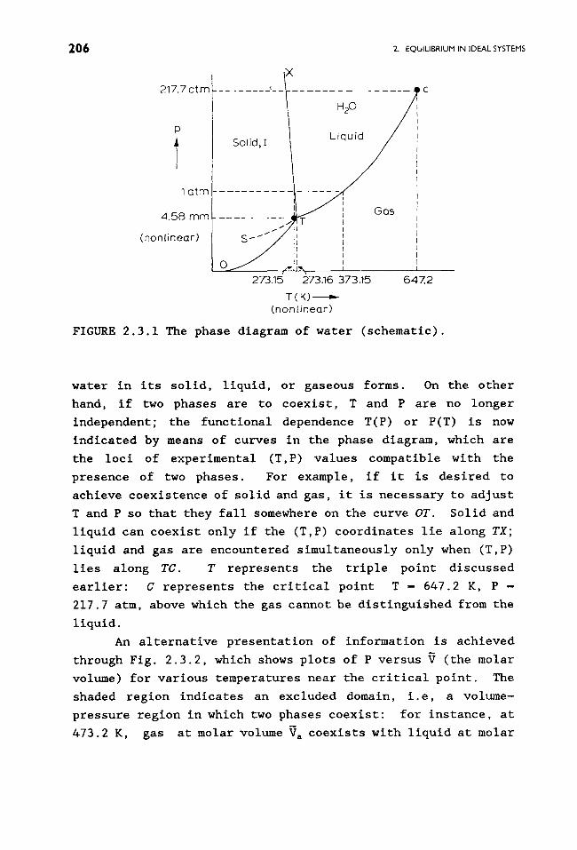
These matters are well summarized pictorially in the
phase diagram for water, Fig. 2.3.1 (not drawn to scale), which
is a representative plot of pressure versus temperature. The
three solid curves separate out three large regions within
which T and P may be altered arbitrarily while maintaining
2 0 6 2. EQUILIBRIUM IN IDEAL SYSTEMS
217.7 a tm
1 otto
4.58 mm
(nonl inear)
X
H20
Solid,/
Gas
I I'~
273.15 273.16 373.15 64Z2
T ( K ) - - - ~ (nonl inear)
FIGURE 2.3.1 The phase diagram of water (schematic).
water in its solid, liquid, or gaseous forms. On the other
hand, if two phases are to coexist, T and P are no longer
independent; the functional dependence T(P) or P(T) is now
indicated by means of curves in the phase diagram, which are
the loci of experimental (T,P) values compatible with the
presence of two phases. For example, if it is desired to
achieve coexistence of solid and gas, it is necessary to adjust
T and P so that they fall somewhere on the curve OT. Solid and
liquid can coexist only if the (T,P) coordinates lie along TX;
liquid and gas are encountered simultaneously only when (T,P)
lles along TC. T represents the triple point discussed
earlier: C represents the critical point T- 647.2 K, P-
217.7 atm, above which the gas cannot be distinguished from the
liquid.
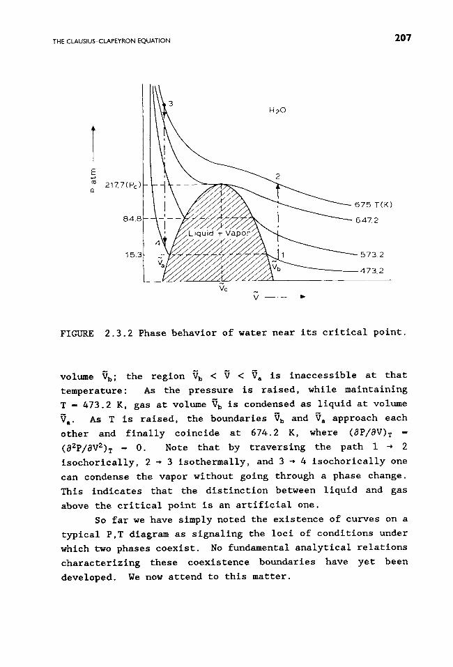
An alternative presentation of information is achieved
through Fig. 2.3.2, which shows plots of P versus V (the molar
volume) for various temperatures near the critical point. The
shaded region indicates an excluded domain, i.e, a volume-
pressure region in which two phases coexist: for instance, at
473.2 K, gas at molar volume V a coexists with liquid at molar
THE CLAUSIUS-CLAPI::YRON EQUATION 2g 7
217.7(Pr
8 4 . 8
15.3
H20
|
675 T(K)
6 4 7 . 2
, . , , , ,
Vc
V ~
FIGURE 2.3.2 Phase behavior of water near its critical point.
volume Vb; the region Vb < ~ < Va is inaccessible at that
temperature: As the pressure is raised, while maintaining
T - 473.2 K, gas at volume Vb is condensed as liquid at volume
Va. As T is raised, the boundaries Vb and Va approach each
other and finally coincide at 674.2 K, where (8P/aV)~ -
(sgP/SV2)T- 0. Note that by traversing the path I ~ 2
isochorically, 2 * 3 isothermally, and 3 * 4 isochorically one
can condense the vapor without going through a phase change.
This indicates that the distinction between liquid and gas
above the critical point is an artificial one.
So far we have simply noted the existence of curves on a
typical P,T diagram as signaling the loci of conditions under
which two phases coexist. No fundamental analytical relations
characterizing these coexistence boundaries have yet been
developed. We now attend to this matter.
~-08 2. EQUILIBRIUN IN IDEAL SYSTENS
As we saw in Section 2.2, equilibrium between two one-
component phases A and B requires equality of the chemical
potentials #A - #S; thus, dPA - d~B.
Therefore,
d#A-_ SAdT A + V^dP A - dPB --- SBdT B + VBdP s . (2.3.:1.)
At equilibrium dT A - dT s - dT, dP A - dP B - dP, whence
(dP/dT) - (S s - SA)/(V s - V^) (2.3.2)
represents the fundamental equation which shows how the
pressure of a two-phase, one-component system changes with
temperature. Now, for a fixed T and P, #B- #A- 0 -- H B - H A -
T(S B - SA) - AH - TAS. It then follows that
(dP/dT) - (AH/TAV), (2 .3 .3)
which is the formulation known as the Clauslus-Clapeyron
equation (1832). Note that AH is the molar enthalpy of
transformation of the system from state A to state B, and
similarly for AV.
Several alternative versions may be found for dealing
with liquid-vapor equilibria" Beginning with the relation
( 2.3.3), it is customary to introduce the following
approximations which may or may not be valid for the particular
case under study (see Exercise 2.3.1)" (i) V I << Vs, (ii) V s --
RT/P. Also, write L v - H s - H e as the molar heat of
vaporization. Then approximately
dP/dT- P~/RT 2 , (2.3.4a)
or
d~n P/dT- ~/RT 2, (2.3.4b)
or
THE CLAUSIUS-CLAPEYRON EQUATION 2 0 9
(d~n P)/d(I/T) -- Lv/R. (2.3.4c)
Equation (2.3.4c) shows that a plot of 2n P versus I/T should
yield a curve with slope - Lv/R. If additionally one assumes
(lii) that L v is independent of T then the above plot yields a
straight llne. In that event Eq. (2.3.4c) may be integrated as
In (P2/PI) - (~/R) ~~2 (dT/T2) -_ (~/R)(I/T2_ I/T1 ) 1
- (t , , , /R) (T2 -T~) /T~T2. (2.3.4d)
Note that any of the equations in (2.3.5) or (2.3.4) specifies
P as a function of T or vice versa. It is not always
recognized that the equilibrium constraints manifested in the
Clausius-Clapeyron equation are commonly employed to fix the
temperature of a helium bath in the range 0.3 to 4.2 K, by
adjusting the vapor pressure of the helium gas above the liquid
phase to correspond to the desired temperature.
Finally, Eq. (2.3.4) is frequently inverted to determine
- RT2(d~n P/dT) - - R[d~n P/d(I/T)]. (2.3.5)
Considerable care must, however, be exercised in the use of
Eqs. (2.3.4) and (2.3.5) because of the many approximations
used in arriving at those particular results.
We briefly consider other aspects relating to the topic
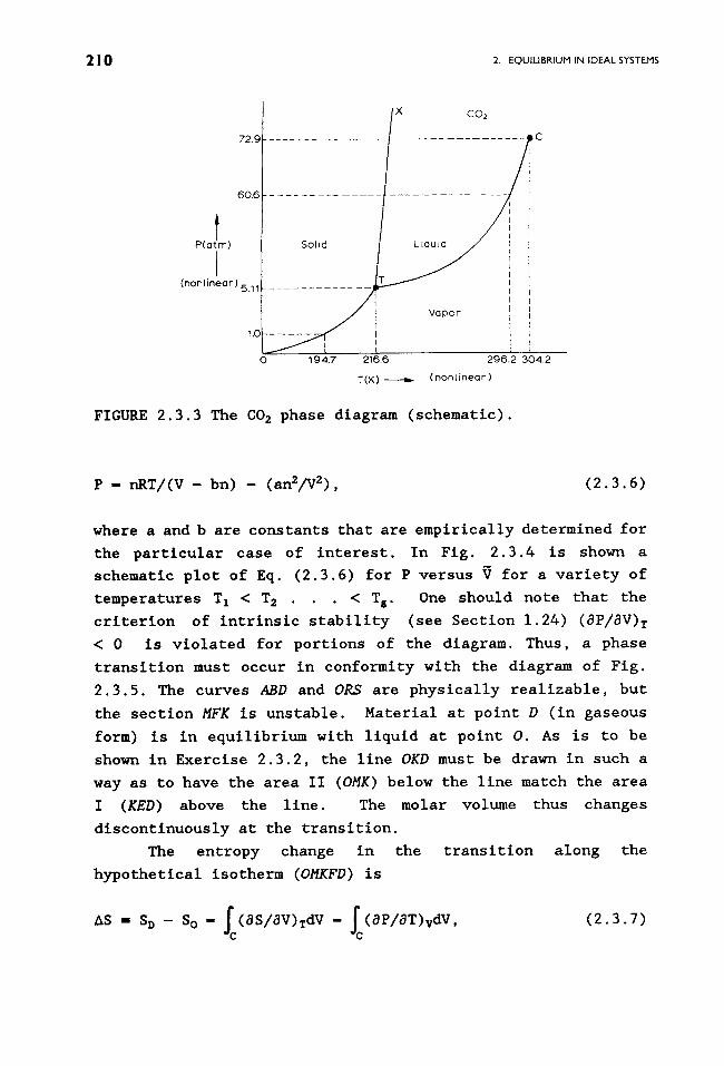
under study. The CO 2 phase diagram is shown in Fig. 2.3.3. In
contrast to the case of H20, the melting curve TX has a positive
slope. This reflects the fact that now V I > V,, whereas for
water (exceptionally) V I < V,. Note further that the triple
point T for CO 2 occurs at 5.11 atm; hence, under ordinary
conditions, solid CO 2 does not melt but vaporizes directly
(i.e. , sublimes from dry ice) into the atmosphere.
The P-V curves in Fig. 2.3.2 are well simulated by use of
the van de r Waals (1879) Equation of State
2 I 0 2. EQUILIBRIUM IN IDEAL SYSTEMS
72.g
60.6
t P(atm)
I (nonlinear) 5.11
1.0
CO2
i Solid ~ Jl
_ _ .
I
i Vapor
L
0 194.7 216.6 296.2 304.2
T(K) ~ (nonlinear)
FIGURE 2.3.3 The CO 2 phase diagram (schematic).
P - nRT/(V - bn) - (an2/V2), (2.3.6)
where a and b are constants that are empirically determined for
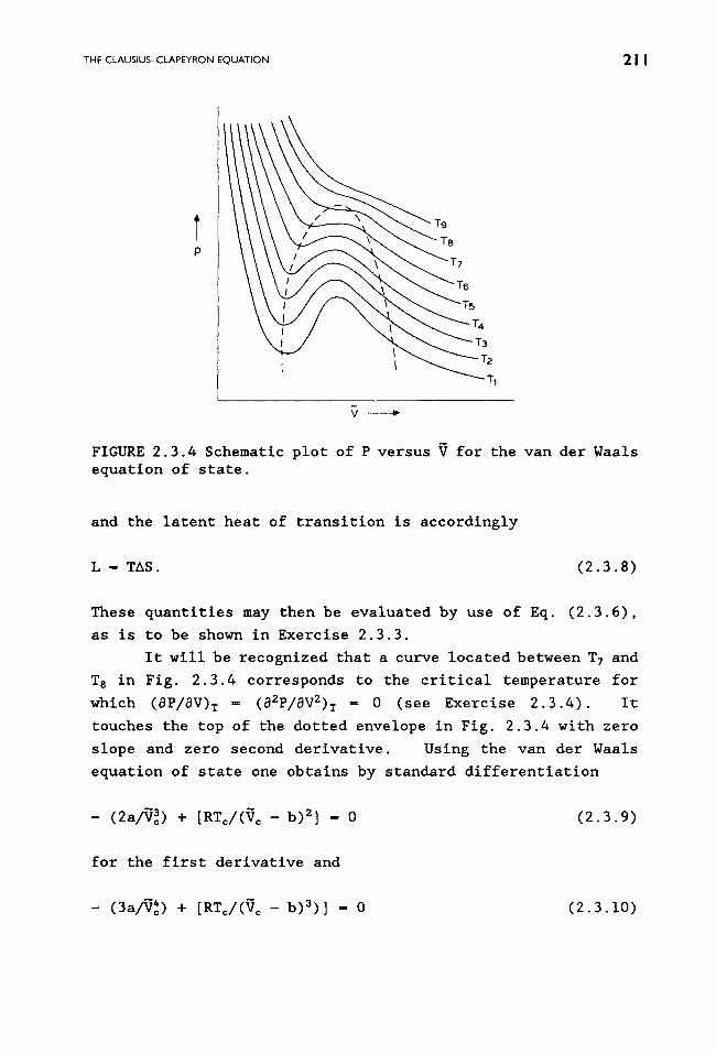
the particular case of interest. In Fig. 2.3.4 is shown a
schematic plot of Eq. (2.3.6) for P versus V for a variety of
temperatures T I < T 2 . . . < T s. One should note that the
criterion of intrinsic stability (see Section 1.24) (aP/av) T
< 0 is violated for portions of the diagram. Thus, a phase
transition must occur in conformity with the diagram of Fig.
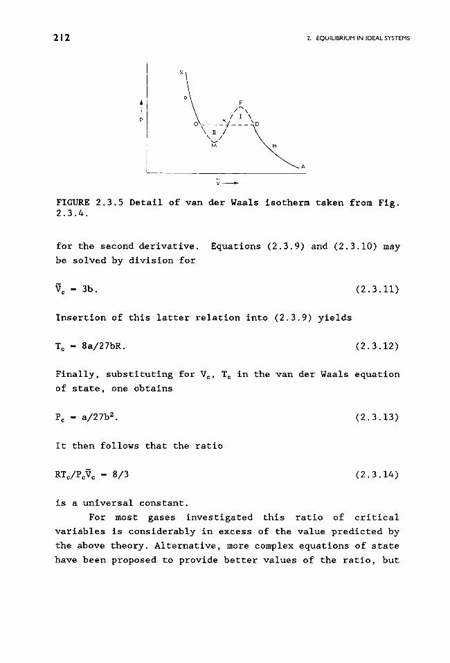
2.3.5. The curves ABD and ORS are physically realizable, but
the section HFK is unstable. Material at point D (in gaseous
form) is in equilibrium with liquid at point O. As is to be
shown in Exercise 2.3.2, the line OKD must be drawn in such a
way as to have the area II (OHK) below the line match the area
I (KED) above the llne. The molar volume thus changes
discontinuously at the transition.
The entropy change in the transition along the
hypothetical isotherm (OMKFD) is
AS- S D - So - fc(aS/aV)TdV - fc (a P/aT) vdV, ( 2.3.7 )
THE CLAUSIUS-CLAPEYRON EQUATION 2 I I
7
TI
V
FIGURE 2.3.4 Schematic plot of P versus V for the van der Waals equation of state.
and the latent heat of transition is accordingly
L- TAS. (2.3.8)
These quantities may then be evaluated by use of Eq. (2.3.6),
as is to be shown in Exercise 2.3.3.
It will be recognized that a curve located between T 7 and
T 8 in Fig. 2.3.4 corresponds to the critical temperature for
which (aP/aV)T = (a2P/aV2) T - 0 (see Exercise 2.3.4). It
touches the top of the dotted envelope in Fig. 2.3.4 with zero
slope and zero second derivative. Using the van der Waals
equation of state one obtains by standard differentiation
- (2a/V~) + [RT=/(V= - b) 2] = 0 (2.3.9)
for the first derivative and
- (3a/V~) + [RTo/(V c -b)3)] = 0 (2.3.10)
~_ | '2 2. EQUILIBRIUM IN IDEAL SYSTEMS
s
?
_K/I I \
\ ~ i - - - - ~ M
~ A
N
FIGURE 2.3.5 Detail of van der Waals isotherm taken from Fig. 2.3.4.
for the second derivative. Equations (2.3.9) and (2.3. I0) may
be solved by division for
V c - Bb. (2.3.11)
Insertion of this latter relation into (2.3.9) yields
T c - 8a/27bR. (2.3.12)
Finally, substituting for V=, T O in the van der Waals equation
of state, one obtains
Pc - a/27b2. (2.3.13)
It then follows that the ratio
RTc/PoV c - 8/3 (2.3.14)
is a universal constant.
For most gases investigated this ratio of critical
variables is considerably in excess of the value predicted by
the above theory. Alternative, more complex equations of state
have been proposed to provide better values of the ratio, but
THE CLAUSIUS-CLAPEYRON EQUATION 213
they are still not entirely satisfactory in describing other
physical properties of real gases.
EXERCISES
2.3.1 Many articles have been published, particularly in the Journal of Chemical Education., dealing with the approximations inherent in the use of Eq. (2.3.4). Look up these articles and write a brief outline presenting arguments which show in what way the approximations cancel each other out and under what conditions the approximations are likely to be applicable.
2.3.2 Present rigorous arguments showing why line OKD in Fig. 2.3.5 must be so drawn that area I matches area II. On what cardinal principle does this case rest?
2.3.3 Using the van der Waals equation of state, determine the entropy change and latent heat for the transition of a substance from the liquid to the gaseous state.
2.3.4 Present arguments to show that at the critical point (aP/aV)T - (a2P/aV2)T - o.
2.3.5 It is desired to prepare a dry-ice-acetone cold bath. (a) How many degrees of freedom exist in the enclosed system? (b) If the pressure over the system is maintained at I atm is the temperature of the bath variable or fixed? Explain why. (c) The CO 2 pressure in equilibrium with solid CO 2 is 792.7 torr and 730.3 torr at -78.0 and -79.0~ respectively. What is the heat of sublimation of CO 2 at-78.50C? (d) How large a change in temperature is produced in the bath by a 30 torr change in pressure near 760 torr? (e) What assumptions are required as regards the calculations in (a) through (d)? In particular, do you make any assumptions concerning physical properties of acetone? What effects are brought about by the presence of air?
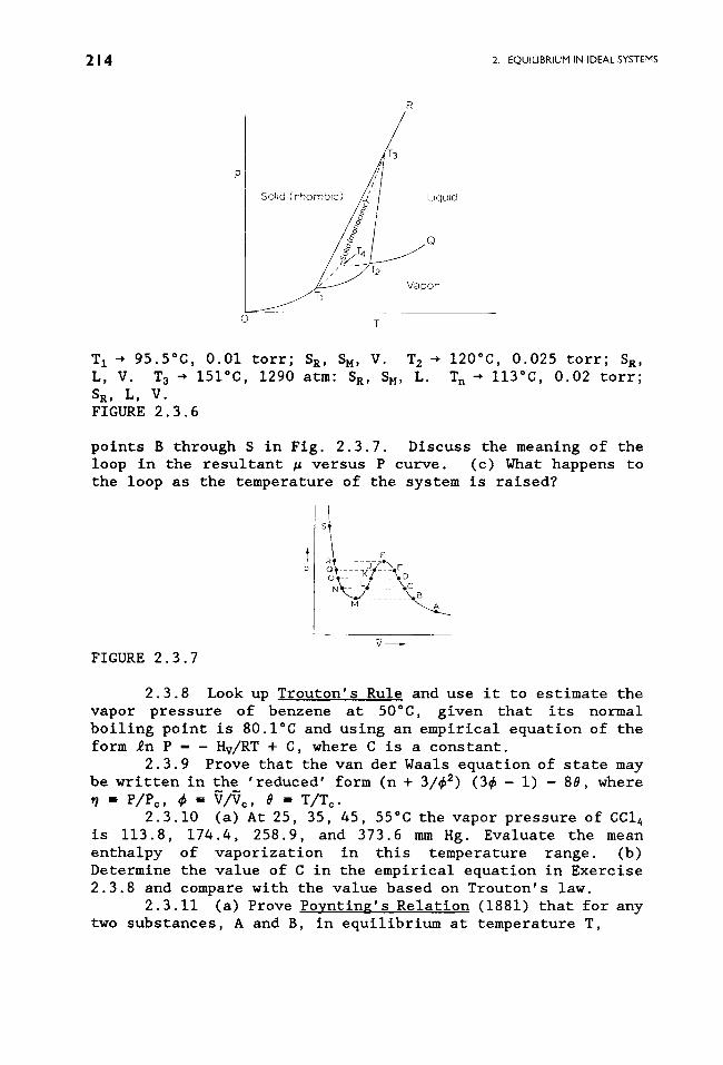
2.3.6 Examine the accompanying graph, Fig. 2.3.6 (not drawn to scale), of the sulfur system. (a) How many triple points are there and how are they labeled on the diagram? (b) Interpret the curve segments OTz, TzT2, TzT 3, TzT 3, T3R, TzT 4, T2T4, T3T4, T2R. (c) How many phases of sulfur are stable under atmospheric pressures? (d) What is the highest pressure at which monoclinic sulfur is stable?
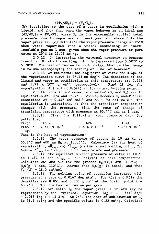
2.3.7 Examine Fig. 2.3.7 which represents an isotherm obtained from the van der Waals equation. (a) Determine # - ~A from the Gibbs-Duhem relation analytically at fixed temperature, where #A is the chemical potential at point A in Fig. 2.3.7. (b) Sketch a plot of # versus P, as obtained from
2 1 4 2. EQUILIBRIUM IN IDEAL SYSTEMS
P
Soltd (rhombf LIqufd
Q
T2 Vapor
T I ~ 95.5~ 0.01 torr; SR, S M, V. T z ~ 120~ 0.025 torr; SR, L, V. T 3 ~ 1510C, 1290 atm: SR, SM, L. T n ~ I13~ 0.02 torr;
S R, L, V.
FIGURE 2.3.6
points B through S in Fig. 2.3.7. Discuss the meaning of the loop in the resultant # versus P curve. (c) What happens to the loop as the temperature of the system is raised?
FIGURE 2.3.7
2.3.8 Look up Trouton's Rule and use it to estimate the vapor pressure of benzene at 50~ given that its normal boiling point is 80.I~ and using an empirical equation of the form 2n P -- Hv/RT + C, where C is a constant.
2.3.9 Prove that the van der Waals equation of state may be written in the 'reduced' form (n + 3/~ 2) (3~ - i) - 88, where
" P/Pc, ~ " V/Vc, 0 - T/T c. 2.3.10 (a) At 25, 35, 45, 55~ the vapor pressure of CCI 4
is 113.8, 174.4, 258.9, and 373.6 mm Hg. Evaluate the mean enthalpy of vaporization in this temperature range. (b) Determine the value of C in the empirical equation in Exercise 2.3.8 and compare with the value based on Trouton's law.
2.3.11 (a) Prove Poynting's Relation (1881) that for any two substances, A and B, in equilibrium at temperature T,
THE CLAUSIUS-CLAPEYRON EQUATION 2 I 5
(OPA/SPB) T = (VB/VA). (b) Specialize to the case of a vapor in equilibrium with a liquid, and show that when the vapor behaves as an ideal gas (dP/dPt) T - PVe/RT , where Pt is the externally applied total pressure, due to vapor and an inert gas, and where P is the vapor pressure. (c) Calculate the vapor pressure change at 25 ~ when water vaporizes into a vessel containing an inert, insoluble gas at 1 arm, given that the vapor pressure of pure water at 25~ is 23.76 mm Hg.
2.3.12 On increasing the external pressure on benzene from 1 to I01 arm its melting point is increased from 5.50~ to 5.78~ The heat of fusion is 30.48 cal/g. What is the change in volume accompanying the melting of 1 tool of benzene?
2.3.13 At the normal boiling point of water the slope of the vaporization curve is 27.15 mm deg -1. The densities of the liquid and vapor at equilibrium at this temperature are 0.958 and 5.98 x 10 -4 g cm -3, respectively. Find AS for the vaporization of 1 tool of HzO(2 ) at its normal boiling point.
2.3.14 Rhomblc and monoclinlc sulfur (S r and Sm) are in equilibrium at 1 atm and 95.4~ When S= becomes S m under these conditions AV- 0.~47 cm 3 tool -I and AH- 90 cal mole -I. The equilibrium is unlvarlant, so that the transition temperature changes with the pressure. Find the rate of change of transition temperature with pressure at 95.4~ and at 1 arm.
2.3.15 Given the following vapor pressure data for palladium" T(K)" 1587 1624 1841 P(mm �9 7.516 x 10 -7 1.614 x I0-6 5.625 x I0 -s
Hg) What is the heat of vaporization?
2.3.16 The vapor pressure of decane is i0 mm Hg at 55.7~ and 400 nun Hg at 150.6~ Calculate (a) the heat of vaporization, ~vap, (b) ASv,p, (c) the normal boiling point, T b. Assume AHva p is independent of temperature and pressure.
2.3.17 The ec[uilibrium vapor pressure of water at IIO~ is 1.414 at and AHva p - 9596 cal/mol at this temperature. Calculate AS ~ and AG ~ for the process H20(2,1 atm, II0~ = H20(g, 1 atm, IIO~ Assume that H20(g ) is ideal, and that VH2 o(~) -- 18.0 cm 3/mol.
2.3.18 The melting point of potassium increases with pressure at a rate of 0.0167 deg atm -I. For K(s) and K(~) the densities are 0.851 and 0.830 g cm -3 at the fusion point t = 63.7~ Find the heat of fusion per gram.
2.3.19 For solid I 2 the vapor pressure in atm may be represented by the empirical equation log P -- 3512.83/T - 2.013 log T + 13.374. At 25~ the heat of sublimation of 12 is 58.6 cal/g and the specific volume is 0.22 cm3/g. Calculate
2 I 6 2. EQUILIBRIUM IN IDEAL SYSTEMS
the molar volume of vapor in equilibrium with 12(s) at 25 and 300 ~ and compare wlth the ideal gas values.
2.3.20 (a) The heat of fusion of ice is 80 cal/g at I atm, and the ratio of the densities of ice to water is 1.091/1. Determine the melting point of ice at I000 arm. (b) For water at 100~ dP/dT- 27.12 mm Hg/deg. Estimate the heat of vaporization.
2.3.21 For solid and liquid HCN the following empirical equations have been cited for the vapor pressure: log P(mm Hg) - 9.33902-1864.8/T (solid); log P (mm Hg) - 7.74460 - 1453.06/T (liquid). Determine (a) the heat of sublimation, (b) the heat of vaporization, (c) the heat of fusion, (d) the triple point and corresponding vapor pressure, (e) the normal boiling point. Is it necessary to assume that all of the latent heats are constant?
2.3.22 The vapor pressures of liquid and solid benzene are cited below: T(K) 260.93 269.26 278.68 305.37 333.15 349.82 P(atm) 1.25xi0 -2 2.39xi0 -2 4.72xi0 -2 0.173 0.515 0.899 The triple point of benzene is at 278.08 K. Determine the enthalpy of vaporization and compare this to the measured value of 30,765 J/tool.
2.3.23 V203 undergoes a metal-lnsulator transition in which the transition temperature can be altered with applied pressure. Experimentally it is found that the variation of transition temperature with pressure is -3.78 x 10 -3 deg/bar and that the change in unit cell volume is 1.5 ~3. The unit cell volume is I00 A (averaged); there are two V203 formula units per unit cell. Calculate the entropy change per mole of V203 involved in the transition.
2.4 PROPERTIES OF IDEAL GASES
(a) An ideal gas is subject to the constitutional equation of
state PV- RT; for a mixture of such gases the equation of
state reads PIV- niRT , or PiVl- RT. One of the consequences
of the third law of thermodynamics, noted in Section 1.21, is
that no real substance with this property can exist for all
conceivable values of P, V, T. However, the ideal gas serves
as a model substance to which real gases approximate at
sufficiently high temperatures and low pressures. We therefore
study the properties of this hypothetical material in detail.
To investigate the thermodynamic properties of ideal
gases, one may insert the constitutional equation of state into
PROPERTIES OF IDEAL GASES 2 I 7
the thermodynamic one, Eq. (1.18.13), to obtain the important
result (aE/aV)~- O. This second criterion is sometimes imposed
as a separate requirement, but such a step is clearly
unnecessary. As an immediate consequence, the general relation
dE- (aE/aT)vdT + (8E/aV)TdV now r e d u c e s to
dE - CvdT. (2.4.1a)
Moreover, for ideal gases
(aCv/aV)=- T[ (a/av)(aE/aT)v]= I T [ (a/aT)(aE/av)=]v- o, (2.4.1b)
which shows that C v can at most be a function of T. We next
appeal to extensive experimental investigations which show that
for noble gases at low pressures and high temperatures C v is
very nearly constant. When this is no longer the case, one
also reaches conditions where the concept of the ideal gas law
begins to break down, in conformity to the Third Law. As a
third criterion for an ideal gas we thus adopt the requirement
that C v be constant: Integration of (2.4.1) then leads to the
result
E- CvT + Eo, (2.4.2)
where E= is the value of the internal energy of one mole of
ideal gas at T -0. As is well known, this latter quantity
cannot uniquely be specified; the energy of any system is known
only to within an arbitrary constant.
Inserting (8E/aV)~ - 0 into Eq. (1.18.17) yields
Cp - C v - P(OV/OT)p - R. (2.4.3)
Accordingly,
H - E + PV - E + RT - (Cv + R)T + E o - CpT + E o. (2.4.4)
It may readily be shown (Exercise 2.4.1) that (8Cp/aP) = O.
2 J 8 2. EQUILIBRIUM IN IDEAL SYSTEMS
The entropy may be found from the Gibbs equation dS -
T-I[dE + PdV] as
dS - (Cv/T)dT + (R/V)dV - C v d~n T + R d~n V. (2.4.5)
On setting PdV + VdP - RdT and substituting for PdV in the
Gibbs equation, one obtains an equivalent expression:
dS - (Cv/T)dT + (R/T)dT - (R/P)dP - Cp d~n T - R d~n P.(2.4.6)
Finally, on introducing the expression d~n T- d~n P + d~n V
into either (2.4.5) or (2.4.6) one obtains
dS - C v d~n P + Cp d~n V. (2.4.7)
These results accord with those of Section 1.17, where a
different approach was provided.
The integration of Eqs. (2.4.5)-(2.4.7) may be carried
through in two equivalent ways. Selecting (2.4.6) as an
example, one may integrate between two specific limits:
I;' s, o' 2 dS" - Cp d 2 n T - R d 2 n P, ( 2 . 4 . 8 ) 1 1
in which S I corresponds to TI, PI and $2, to T2, Pz. For
i l l u s t r a t i v e p u r p o s e s we c o n t i n u e t o c o n s i d e r t h e c a s e w h e r e Cp
is independent of T. In such circumstances
S 2 - S I + Cp ~n (Tz/T I) - R ~n (Pz/PI). (2.4.9)
If one selects TI and PI as reference values and allows $2, T2,
P2 to be arbitrary then Eq. (2.4.9) specifies the molar entropy
of an ideal gas relative to the entropy for the gas in a state
characterized by (TI,PI). It is convenient to set T I - i; PI-
I, in which case Eq. (2.4.9) simplifies to
S - S I + Cp ~n T- R ~n P, (2.4.10)
PROPERTIES OF IDEAL GASES 2 1 9
in which it is implied that T and P are specified in the same
units as TI(K) and PI; here the standard state refers to T- I
K and P - I arm.
(b) It is instructive to proceed by an alternative route.
Equation (2.4.6) may be integrated so as to obtain (2.4.10)
directly, in which case S I represents the entropy at T - P - I
(note that S I is not the value of S at T -0!). Here, one seems
to run into a problem of dimensional analysis, since Eq.
(2.4.10) involves quantities in the argument of the logarithms
that are not pure numbers. There are two distinct though
interrelated methods of getting around this difficulty. The
first is to identify S 2 - Cp in T 2 - R in P2 and S I - Cp ~n T I +
R ~n PI in Eq. (2.4.9). We then see that if we alter the units
of P2 we must simultaneously change those of PI. Thus, the
difference S 2 - S I is unaffected by such a change in units. One
thereby recovers an equation of the form (2.4.10), which is now
seen to depend only seemingly on the chosen units of P. This,
however, obscures the following important point" Self-
consistency in the structure of Eq. (2.4.10) demands that S I -
~n ~, where ~ has the dimension of P~/T% = (P/TS/2). Then the
problem of units and dimensions disappears once again" with S I
- ~n ~, S does not, in fact, depend on the dimensions adopted
for T and P in the arguments of the logarithmic terms (though
S manifestly depends on the choice of units for C e and R which
are multipliers of ~n T and ~n P). Consequently, any change in
units in ~n P or ~n T must be counterbalanced by a
corresponding change in S I" In like manner, S is found to be
independent of the units adopted for T, P, or V in the
logarithmic arguments of Eqs. (2.4.5), (2.4.7), or (2.4.10).
For a definitive proof that S I has the properties just described
one must turn to the methodology of statistical mechanics.
To review and summarize" While the terms ~n V and ~n P do
depend on the set of units which is selected, the quantity S I
does likewise, and in such a compensating manner that the
algebraic sum in (2.4.10) is independent of the units used in
the logarithmic arguments. We have thus arrived at the
2 2 0 2. EQUILIBRIUM IN IDEAL SYSTEMS
relations (2.4.10) and at their equivalent forms which hold
for ideal gases, namely,
S - S 1 + C v 2 n T + R 2 n V (2.4. lla)
S - S 1 + C v 2 n P + Cp 2 n V. (2.4. llb)
To apply these relations to actual gases it may in certain
cases be necessary to replace terms such as Cp 2n T by ;Cp(T)
d2n T and to specify the dependence of Cp on T.
(c) We next determine the Gibbs free energy for a single
gas species according to
G - H- TS - CpT + E o - T(Cp 2n T- R 2n P + SI)
-G I + RT 2n P, (2.4.12a)
in which we have set
G I - E o - TS I - CpT 2n T + CpT. (2.4.12b)
From earlier discussion it should be evident that G - ~ is the
chemical potential of the ideal gas; G I is a reference chemical
potential which depends solely on T.
Equation (2.4.12a) is so important a relation that it is
desirable to rederive it on the basis of a slightly more
generalized approach, for a mixture of ideal gases. We begin
with Eq. (I.18.7), which in the present case reads (aG/aP)T- v - 7.cj)njRT/P. By partial differentiation with respect to nl,
this latter equation may be brought into the form
(a.~/aP)~ I V I RT/P. (2.4.13a)
Next, we take note of the chain differentiation (@~I/@P)T-
(@~I/SPI)T(SPI/SP)T and of the equation Pi = xiP. The preceding
relations show very clearly the need to distinguish between the
PROPERTIES OF IDEAL GASES 2 2 I
partial pressure Pi exerted by gas i and the total pressure P
that is the sum of the partial pressures. Equation (2.4.13a)
may now be recast as
(8~i/SPi)~ - RT/Px i - RT/PI, (2.4.13b)
and this may be integrated as
Pi d~,ilT - RT d2n PIIT '~Pi
(2.4.14a)
to yield
~i(T,Pi) - ~I(T,P~) - RT(~n Pi - 2n P~). (2.4.14b)
Let us choose for P~ some standard pressure such as I atm. In
this particular situation #i(T,l) w #~P(T) may be considered as
a s.tandard chemi.cal potential. Thus, Eq. (2.4.1b) becomes
~t(T,Pt) - ~P(T) + RT 2n Pi. (2.4.15)
This result may be reformulated by use of the relations,
applicable to ideal gases, namely, Pi - cIRT - xIP- Then
~i(T,c i) - ~=(T) + RT 2n cl, (2.4.16)
where ~C(T) -~P(T) + RT ~n RT; alternatively,
#i(T,P,x i) - ~X(T,p) + RT ~n x i, (2.4.17)
where ~X(T,P) - ~P(T) + RT 2n P. Note that while ~P and ~=
are (parametric) functions of T alone, ~x depends as well on
the total pressure P. Here the question of units may again be
raised. It appears from (2.4.12) and (2.4.15), (2.4.16),
(2.4.17) as if the value of ~i depended on the choice of units
selected for Pi; the appearance of the ~n T term in (2.4.12b)
is similarly troublesome. We can dispose of these difficulties
in the same manner as before, but one must now carefully
2 2 2 2. EOU~UBRIUM ,N ~DEAL SYSTEMS
consider several effects : (i) Because the arbitrary reference
energy E o enters Eq. (2.4.12), #i is, in fact, known only to
within an arbitrary constant; this is as expected for a
quantity that represents a generalized energy. (ii) The
standard chemical potential in (2.4.15), ~P, involves
logarithmic terms via S I that eliminate the spurious dependence
of ~i on the units for P and T in the arguments of the
logarithms. If a different set of units is adopted, ~P and ~c
automatically are altered in such a way as to compensate for
such changes. (ill) Finally, the numerical values of ~i are
obviously affected by the units selected for R and for Cp, which
occur as terms in (2.4.12a) or as multipliers of the
logarithmic functions in (2.4.12b). Once more, we note that
~P(T) is the value of ~i when one sets Pi = i in any desired
system of pressure units; normally the value of P• - i atm is
adopted as the standard pressure at the temperature T of
interest.
Equations (2.4.15)-(2.4.17) serve as prototype
expressions for chemical potentials in other types of systems
discussed later and will be referred to as canonical forms.
EXERCISES
2.4.1 (a) For a perfect gas prove that (SCp/SP)T-~ O. (b) Show under what conditions Cp is independent of T as well.
2.4.2 Define the Gibbs free energy density g by gV--G. From the relation V- (SG/SP)T derive a differential equation involving (Sg/SP)T. Solve this equation for g(P) at fixed T. Prove that the resultant equation is equivalent to ~ - ~o + RT 2n P for the case of a perfect gas. Note that the solution of the differential equation is simplified by introducing the isothermal compressibility ,8 where appropriate. Compare and contrast g(P) for a perfect gas with g(P) for a condensed material where ,8 may be regarded as sensibly independent of P.
2.4.3 (a) Derive the equation of state for an ideal gas from the formula for the chemical potential ~• (b) Calculate the change in chemical potential of component i of an ideal gas mixture, under an isothermal reversible expansion from i to I0 liters.
PROPERTIES OF IDEAL SOLUTIONS IN CONDENSED PHASES 2,2,:3
2.5 PROPERTIES OF IDEAL SOLUTIONS IN CONDENSED PHASES
We proceed by analogy to Section 2.4 to establish the
thermodynamic properties of ideal solutions forming a condensed
phase in equilibrium with the vapor phase. $.dea! s01ut.lons are
defined to be those mixtures forming a single, homogeneous
phase which satisfy three criteria" (a) There shall be no
volume change in forming the solution from its individual
components" Let V i be the molar volume of pure i and Vi, its
partial molal volume in solution. Then the combined volume of
all constituents prior to mixing is Z(1)nlVl, and the volume of
solution after mixing is Z(1)nlV i. For ideal solutions AV ..- m ~'t
Z(1)ni(V i -V~) -0, i.e., V I -V i for every i. (b) There shall
be no enthalpy change in the mixing process" Let H i and H i be
the molar and partial molal enthalpies of component i in pure
form and in the final solution respectively. Then the combined
enthalpy of all constituents prior to mixing is E(1)niH ~ and the
total enthalpy of the solution is Z(1)niH i. For ideal solutions
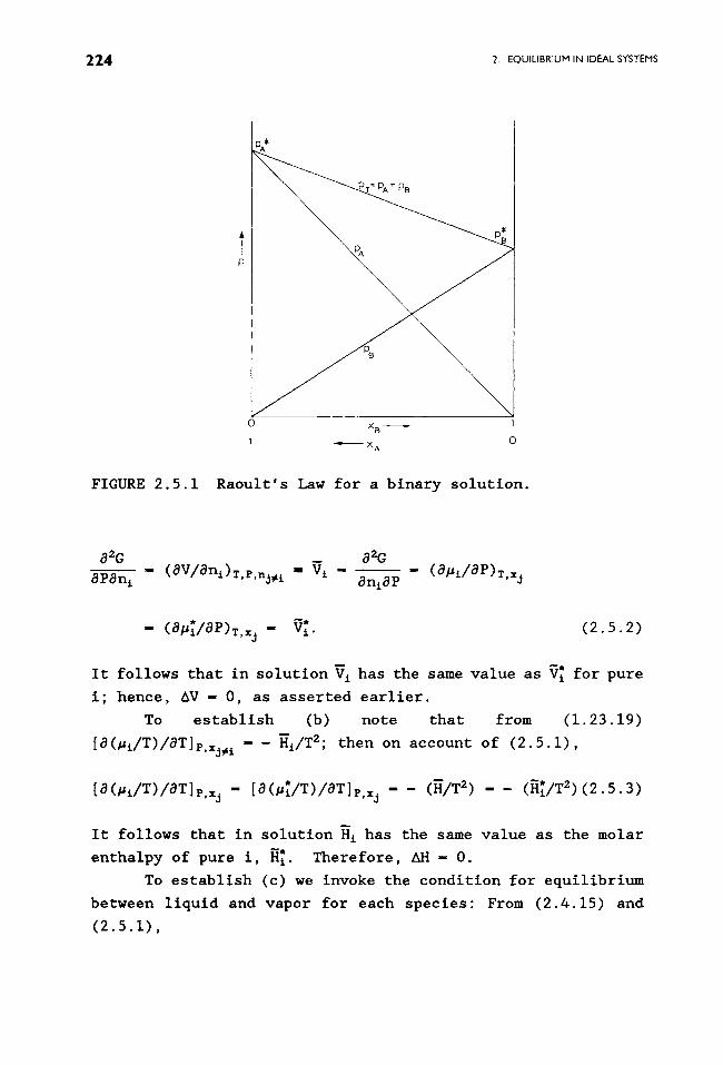
All - E(1)ni(H i - H i ) - 0, i.e. H i - H i for every i. (c) Raoult's
Law shall be obeyed" For each component the partial pressure
of species i in the gas phase in equilibrium with the solution
is given by Pi -xIPi, where x i is the mole fraction of species
i in the condensed phase and P[ is the equilibrium vapor
pressure of i over pure liquid i. An illustration of Raoult's
law for a binary phase is furnished by Fig. 2.5.1. The
asterisks refer to properties of pure condensed phases.
We now show that criteria (a)-(c) are met by postulating
the following canonical form for the chemical potential of each
species in the ideal solution"
~i - #I(T,P) + RT 2n x i. (2.5.1)
Observe that ~i is the chemical potential of pure liquid i, when
x i - i, ~i i #i, this latter quantity depends parametrically on
T and P.
To establish criterion (a) note that (aG/aP)T,xj -V and
(aG/anl)~,P,nj# i " ~i. Hence,
~ . , , 4 2. EQUILIBRIUM IN IDEAL SYSTEMS
O XB.----_~ 1
1 ...,------ XA O
FIGURE 2.5.1 Raoult's Law for a binary solution.
82G _ 82G 8 P a n i I ( S V / a n i ) T p , n 3 ~ i ! V i - - - - ( 8 / ~ i / 8 P ) T xj
' 8 n i 8 P ,
- (a#*~/aP)~,~j- vi. (2.5.2)
It follows that in solution V• has the same value as V i for pure
i; hence, AV I 0, as asserted earlier.
To establish (b) note that from (1.23.19)
[8(#i/T)/aT]p,xj~i I _ ~• then on account of (2.5.1),
[a(~jT)/aT]p,x j I [a(#~/T)/aT]p,~j I - (H/T 2) -- (H~/T2)(2.5.3)
i i
It follows that in solution H i has the same value as the molar
enthalpy of pure i, H i . Therefore, AH I 0.
To establish (c) we invoke the condition for equilibrium
between liquid and vapor for each species: From (2.4.15) and
(2.5.1),
PROPERTIES OF IDEAL SOLUTIONS IN CONDENSED PHASES ~-~-5
~P(T) + RT ~n Pi - #I(T,P) + RT ~n x i. (2.5.4)
Hence, at constant T and total pressure P,
2n Pi - - (I/RT)(#~P- #~) + ~n x i. (2.5.5)
Now the first term on the right is constant as long as T and P
are held fixed; hence, (2.5.5) is equivalent to Pi -Cxl, where
C is a 'constant' that is evaluated by requiring that for x i -
�9 * whence Raoult's Law �9 then C - Pi, i, Pi - Pi,
Pi i xip~ (2.5.6)
is satisfied.
Thus, the canonical form (2.5.1) does indeed meet the
requirements (a)-(c) for ideal solutions. Equation (2.5.1)
represents one of the most basic relationships in chemical
the rmo dynam i c s.
From (2.5. I) one can immediately derive various
thermodynamic quantities of mixing" Let G be the Gibbs free
energy of the solution and G i be the molar Gibbs free energy of
the !th pure component. Then
- niC i ni[#t + RT ~n xi] - ~ n• i AG(T,P) - G ~i " * - l
- RT ~ n i 2n x i. (2.5.7) i
On defining AG ~ AG/~(• i one obtains the more symmetric
relation
AG - RT x i ~n x i . (2.5.8)
As shown earlier, All - 0; hence, AS - - AG/T. Thus, we obtain
AS - - R x i ~n x i. (2.5.9)
Note further that with AV - 0, AE - All- PAV i 0; thus ACp - 0.
~6 2. EQUILIBRIUM IN IDEAL SYSTEMS
Before proceeding we add a word on nomenclature" When
Eq. (2.5.1) is specialized by setting P- 1 arm; ~ (T,I) is
termed a standard chemical potential; for other pressures, we
shall refer to ~I(T,P) as the reference chemical potential,
Concentration in solution is often measured in terms of
molarlty c i or molallty m i; hence, the chemical potentials of
species i are frequently rewritten as
~i(T,P,cl) - ~i(T,P,c i - I) + RT ~n c i (2 .5 .1o)
~,(T,P,ml) - ~i(T,P,ml - I) + RT 2n m i. (2.5.11)
These relations reduce to an identity for c i - i or for ml - i,
and the reference chemical potentials now relate to a solution
in which species i is present at unit molarity or molality. The
problem of dimensions again comes up here and must be disposed
of as in Section 2.4. This points up the desirability of
introducing another set of equations for specifying chemical
potentials, namely,
~i(T,P,cl) -~I(T,P,c~) + RT 2n [cI(T,P)/c~(T,P)] (2.5.12)
~i(T,P,m i) - #i(T,P,m~) + RT 2n [m• (2.5.13)
Here c i and m i are the molarlty and molality of i in its pure
state as specified in Eqs. (3.5.2) of Chapter 3. For c i - c i
and m i -m~ the preceding relations reduce to an identity. The
problem of dimensionality now does not arise; further, the
reference potentials now relate once more to species i in its
pure state. It is thus unfortunate that the canonical forms
(2.5.10) or (2.5.11) rather than the relations (2.5.12) or
(2.5.13) have historically been adopted as a starting point.
Several points are relegated to exercises" In Exercise
2.5.1 it is to be shown how (2.5.12) and (2.5.13) may be
derived from (2.5.10) and (2.5.11) and how ~i(T,P,c~),
~i(T, P,m~) are related to ~i(T, P, c• and ~i(T, P,mi-l),
respectively. Using results derived in Section 2.10, Exercise
PROPERTIES OF IDEAL SOLUTIONS IN CONDENSED PHASES 227
2.5.3 calls for interrelations between ~i(T,P,c~), ~•
and ~i(T,P,xi-(c). Further insight may also be gained by
referring to Chapter 3, where these matters are taken up in
great detail for nonideal solutions.
Note further that Eqs. (2.5.1), (2.5.12), and (2.5.13)
remain self-consistent if in place of #i(T,P,x~), ~i(T,P,c[), or
pi(r, P,m~) one were to use ~i(r, l,x~), (pi(r, i, c~), and
xi(T,l,m~). The revised equations read
~i(T,P,xl) - ~i(T,l,x~) + RT ~nx i (2.5.14)
~i(T,P,cl) - ~i(T,l,c~) + RT ~n[ci(T,P,)/c~(T,l)] (2.5.15)
~i(T,P,ml) - ~i(T, l,m~) + RT2n[ml/m~] , (2.5.16)
which reduce to an identity when x i - x~, P - I; or c i - c~, P
- I; or m i - m~, P - I. The advantage of the preceding
relations is that all ~i's are specified relative to a single
standard chemical potential, namely that which obtains at unit
pressure (usually, i arm).
For the present, we confine ourselves to use of Eq.
(2.5.1) in developing further results.
EXERCISES
2.5.1 Derive Eqs. (2.5.12) and (2.5.13) from (2.5.10) and (2.5.11), respectively by specializing, as an intermediate step, to the case of a pure material of 'molarity' c i and ' molality' m~.
2.5.2 Obtain specific relations for c~ and m~ from first principles or by specialization of Eqs. (2.10.7) and (2.10.9).
2.5.3 By equating (2.5.1) with (2.5.10) and (2.5.11) and specializing to the case of pure materials, derive relations between (T,P,c~), ~i(T,P,m~), and ~i(T,P,x~).
2.5.4 Construct graphs of AG/RT, AS/R, and AH against x I and x z for a formation of a binary solution, and discuss the significance of the curves. At what point do AG and AS assume their largest numerical values, and what are the corresponding values of AG/RT and AS/R?
2.5.5 (a) Find AG, AV, AS, AH, AE, and AF when dissolving 2.0 tool of SnCI4(~) in 3.0 tool of CC14(~ ) at 298 K
2 2 8 2. EQUILIBRIUM IN IDEAL SYSTEMS
and i atm to produce an ideal solution. (b) If the entropies of SnC14(2 ) and CC14(2) under these conditions are 61.8 and 51.3 eu mole -I, respectively, find the entropy of the solution formed in (a). (c) Find the partial molal entropy of SnCI 4 in in (a).
2.5.6 One liter of O 2 and 4 liters of N 2, each at i arm and 27~ are mixed to form an ideal gas mixture of 3 liters at the same temperature. Calculate AG, AS, and AH for this process.
2.6 THE DUHEM-MARGULES EQUATION AND ITS CONSEQUENCES
(a) An interesting consequence of the Gibbs-Duhem equation
(Section 1.22) for a two-component system is developed in this
section. We divide nld~i + n~d~2 " 0 with (n I + n2) to find xld~i
+ x2d~2 - 0. At constant T and P, d~i - (@~i/@Xl)T, P dxl, whence
X1(apl/aXl)T, P dx I + X2(a~2/apZ)T, P dx 2 - 0 (T,P fixed), (2.6.1)
or
(a~I/a2n XI)T, P dx I + (a~2/@~n X2)T, P dx 2 - O. (2.6.2)
Since x I + x 2 - i, dx I + dx 2 - 0; Eq. (2.6.2) thus simplifies to
(a,~I/a2n Xl)T, P -- (apa/a2n X2)T, P -- 0. ( 2 . 6 . 3 )
Finally, on introducing the relation d#ilT.e- RT d2n Pi for
gases we obtain
(8~n P1/a2n Xl)T, P -- (a2n P2/a~n X2)T, e, (2.6.4)
which is the Duhem-Margules equation (1886, 1895).
(b) An immediate consequence of the preceding relation is
that if Raoult's law applies to one component of a binary
mixture, it must apply to the second as well. Suppose that for
component I, PI - xiP~, since at constant T, P the quantity PI
is fixed, (a2n P1/a2n Xl)T,p- i. By (2.6.4) we then also have
THE DUHEM-MARGULES EQUATION 229
(82n Pz/82n x2)T, P - I, whence integration yields P2 - xP~, as
was to be proved.
One observes that in the vapor phase
P = xxP' ~ + x2P 2 = xxP 1 + (1 - x l ) P 2 P2 + x I ( P 1 - P2)
- P1 + x 2 ( P 2 - P1) , ( 2 . 6 . 5 )
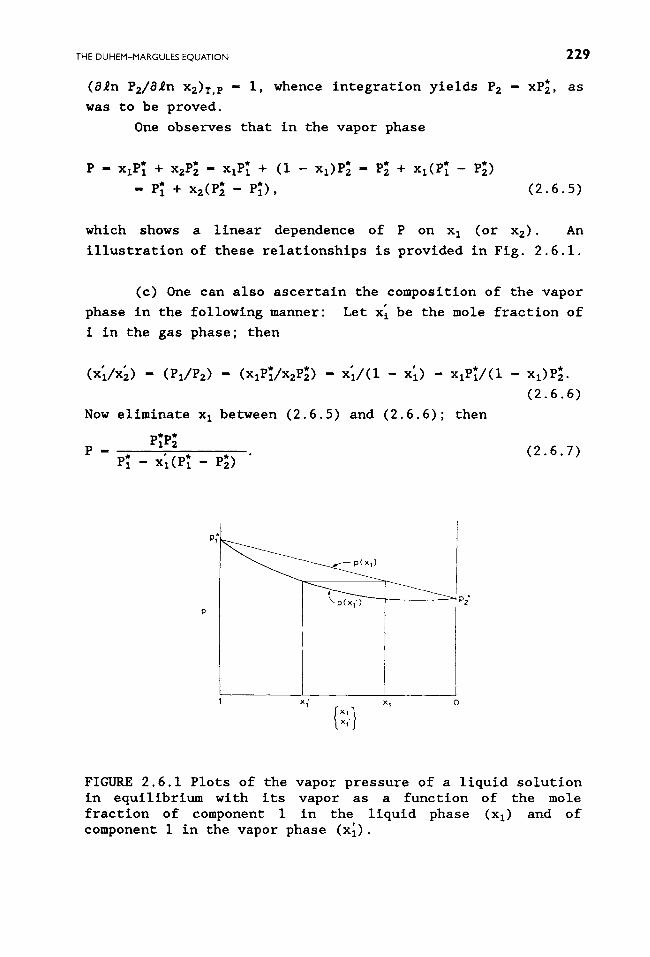
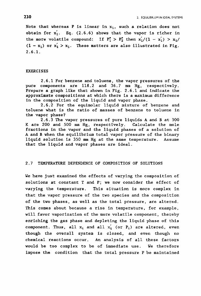
which shows a linear dependence of P on x I (or x2). An
illustration of these relationships is provided in Fig. 2.6.1.
(c) One can also ascertain the composition of the vapor
phase in the following manner" Let xl be the mole fraction of
i in the gas phase; then
(xl/x2) - (PI/P2) - (xIP~/x2P~) - xl/(l - xl) - xIP~/(l - xl)P~.
Now eliminate x I between (2.6.5) and (2.6.6); then
( 2 . 6 . 6 )
t~ ~r P1P2
Px - x:(P1 - P~) (2.6 7)
p~
1 X 1' X 1 O
FIGURE 2.6.1 Plots of the vapor pressure of a liquid solution in equilibrium with its vapor as a function of the mole fraction of component I in the liquid phase (xl) and of component i in the vapor phase (x'1).
~ , ~ 2. EQUILIBRIUM IN IDEAL SYSTEMS
Note that whereas P is linear in xl, such a relation does not
obtain for x I. Eq. (2.6.6) shows that the vapor is richer in
the more volatile compound" If PI > P2 then xl/(l - xl) > xl/
(i - x I) or xl > x I. These matters are also illustrated in Fig.
2.6.1.
EXERCISES
2.6.1 For benzene and toluene, the vapor pressures of the pure components are 118.2 and 36.7 Hg, respectively. Prepare a graph llke that shown in Fig. 2.6.1 and indicate the approximate compositions at which there is a maximum difference in the composition of the liquid and vapor phase.
2.6.2 For the equimolar liquid mixture of benzene and toluene what is the ratio of masses of benzene to toluene in the vapor phase?
2.6.3 The vapor pressures of pure liquids A and B at 300 K are 200 and 500 mm Hg, respectively. Calculate the mole fractions in the vapor and the liquid phases of a solution of A and B when the equilibrium total vapor pressure of the binary liquid solution is 350 mm Hg at the same temperature. Assume that the liquid and vapor phases are ideal.
2.7 TEMPERATURE DEPENDENCE OF COMPOSITION OF SOLUTIONS
We have just examined the effects of varying the composition of
solutions at constant T and P; we now consider the effect of
varying the temperature. This situation is more complex in
that the vapor pressure of the two species and the composition
of the two phases, as well as the total pressure, are altered.
This comes about because a rise in temperature, for example,
will favor vaporization of the more volatile component, thereby
enriching the gas phase and depleting the liquid phase of this
component. Thus, all x i and all x i (or Pi) are altered, even
though the overall system is closed, and even though no
chemical reactions occur. An analysis of all these factors
would be too complex to be of immediate use. We therefore
impose the condition that the total pressure P be maintained
TEMPERATURE DEPENDENCE 23 I
constant. Experimentally this may be achieved by having
present in the gas phase a third, nonreactive gas that does not
appreciably dissolve in the solution. As T is altered, the
neutral gas is either metered in or else withdrawn in
increments (through a semipermeable membrane) as needed to
maintain the overall P values. Alternatively, the solution is
encased in a pressure vessel with a moveable piston, which is
readjusted so as to maintain a constant overall pressure.
We invoke the equilibrium constraint for each species:
#i(g) - #i(~) " Then (~ - ~P of Section 2.4)
#~/RT + 2n P i - #~/RT + 2n xl, ( 2 . 7 . 1 )
so that for the contemplated changes
[ (a/aT)(/~/RT) ]p + (a2n Pt/aT)p I [ (a/aT)(#~/RT) ]p + (a2n x~/aT)p. (2.7.2)
Now let xl designate the mole fraction of i in the vapor phase;
then Pi - xIP. It follows that (8~n Pi/gT)p- (8~n xl/OT)p. We
t h e n f i n d
a - a _ _ - * - _ _ -
RT RT 2 RT 2 " x i ) p P
(2.7.3)
Here we first utilized Eq. (2.5.3) and then introduced the
second criterion for ideal gaseous and liquid solutions,
whereby the molar enthalples for the pure components, H i and H~,
are equal, respectively, to the partial molal enthalpies of the
same constituent in solution (Hi) and in the vapor phase (Hi).
Notice that the preceding derivation can also be applied
to any two-phase mixture such as two sets of immiscible
liquids, a llquld-solld system, or two types of solid
solutions. In these cases the dashed and undashed quantities
refer to the two respective phases. For the special case of a
solution in equilibrium with a pure solid the dashed quantities
2 3 2 2. EQUILIBRIUM IN IDEAL SYSTEMS
x i remain constant and Eq. (2.7.3) then reduces to the form
(8~n xl/ST)p,xj -AH~/RT z where AH~ is the enthalpy of fusion for
component i which freezes out as a pure solid.
2 .8 LOWERING OF THE FREEZING POINT AND ELEVATION OF THE
BOILING POINT OF A SOLUTION
(a) One of the interesting problems in solution thermodynamics
is the change in freezing and boiling points of a solvent to
which a solute has been added. Extensive experimentation has
shown that the addition of a material B that dissolves in
liquid A causes a lowering of the freezing point of A; for
example, A and B may represent water and sugar, respectively.
We look for an analytic relation that shows how much the
freezing point is depressed when a given quantity of solute is
dissolved in the solvent.
We consider a two-phase system consisting of pure solid
A (e.g., ice) in equilibrium with the solution of B dissolved
in liquid A (e.g., sugar in water). This requires the equality
of the chemical potential ~A in both phases:
,A' ~, ~A(T,P) - ~z(T,P) + RT ~n xz, (2.8.1)
where #A and #z are the chemical potentials of pure A in the
solid and in the liquid state, respectively.
One should note the implication of the equilibrium
condition (2.8.1). At constant P, a given temperature
corresponds to particular composition, xz, of the solution, and
vice versa. Thus, x z becomes a function of T; x z - xz(T). To
investigate this dependence further it is ~ propos to subject
(2.8.1) to partial differentiation with respect to T"
- { a [ ( ~ - ~ , ) / R T ] / a T } p - ( ~ - ~ ) / R T : ' ,, E~/RT:' - (a.~n x z / a T ) p .
(2.8.2) In this expression we have first invoked Eq. (1.23.19) or,
alternatively, (2.7.3) in different notation; H z and H A are the
CHANGES IN FREEZING AND BOILING POINTS 233
molar enthalples of pure liquid A and pure solid A. These
quantities enter here because they correspond to #i and ~a,
respectively. Next, we have defined L~ as the molar heat of
fusion of pure A; note that this is not the molar enthalpy
change accompanying the transfer of pure A into the solution
AB. Lastly, we invoked Eq. (2.8.1) to obtain the quantity on
the right. Note again that x I depends implicitly on T; see
Exercise 2.8.1.
Equation (2.8.2) may be rewrltten as
i d~n x I - - (~.~/RTa)dT, (P constant) (2.8.3) f
where the limits on the integral correspond to two different
situations" T~ is the freezing point of pure A (x I - I) and T I
is the freezing point of the solution for whfch the mole
fraction of A is x I. In Exercise 2.8.1, we pose the problem as
to why a change in T should result in a change in composition.
We introduce a temperature dependence of L~ in first order
through use of the Kirchhoff relation, Section 1.18, (OL~/aT)p
- (Cp) I - (Cp) A ACp, in which ACp represents the difference in
molar heat capacity of pure liquid A and pure solid A. Under
the assumption that the variation of ACp with T may be ignored,
we find
L~- L~ + ACp(T - Tf), (2.8.4)
where L~ is the value of Lf at T - Tf. Thus,
~:Id2n x l - - .[TT~ [E~/RT 2 + (ACe/RT2)(T- T~)]dT (P constant).
(2.8.5)
Define the lowering of the freezing point by
8 f - T~- TI, (2.8.6a)
so that
T1 - T ~ [ 1 - ( e ~ / T ~ ) ] . (2.8.6b)
2 3 4 2. EQUILIBRIUM IN IDEAL SYSTEMS
Equation (2.8.5) may then be integrated to yield
- ~n xll P - [ (L~/RTf) - (ACp/R) ] (Tf - TI)/T I - (ACp/R)2n (TI/Tf) ]p
- [(L~/RTf) - (ACp/R)] [Of/Tf(l - Of/Tf)]
- (BOp/R) 2n [1 - (O~/Tz)llP. ( 2 . 8 . 7 )
In general it is an excellent approximation to expand in
small powers of 0f/Tf" We obtain (I - Of/Tf) -I = I + Of/Tf + ...
and 2n (i - Of/Tf) = - [Of + O~/2T~ + ...]. Further, - 2n x I -
-2n (i- x 2) --x 2. Equation (2.8.7) then reduces to
x 2 = (~.~/RTf)(ez/Tz) + [ (E~/RTf) - (n~p/2R)] (ez/Tz) 2. (2 .8 .8 )
The replacement of- 2n x I by x 2 does limit the applicability of
Eq. (2.8.8) to dilute solutions, but this limitation is clearly
essential if the theory of ideal solutions is to be applicable
to real cases.
Equation (2.8.8) is a quadratic equation in 8f which may
be solved to find 8f in its dependence on x 2. However, in view
of all of the above approximations it is generally appropriate
to neglect the term in (Sf/Tf) 2. Equation (2.8.8) may then be
inverted to read
O f - (RT~/E~)x 2. ( 2 . 8 . 9 )
Ordinarily, the lowering of the freezing point is
expressed in terms of the molality m 2 of the solute. We note
that m 2 - I000 n2/nIM1, where M I is the gram molecular weight of
the solvent" further, x 2 - n2/(n I + n2) = n2/n I. Hence, x2/m 2 =
MjI000 for dilute solutions. Thus,
Of = (RT2fMjI000 ~.~)m 2 - Kfm 2. (2.8.10)
This relationship is rather remarkable in several
respects. First, in the approximation scheme used here the
lowering of the freezing point is a linear function of x 2 or m 2.
Second, the proportionality factor is dependent solely on the
CHANGES IN FREEZING AND BOILING POINTS 2 3
properties of the pure solvent (i.e., on M1, Tf, L~) and in no
way depends on the properties of the solute. For a fixed
solvent Kf is thus predetermined and is maximized for solvents
with high freezing points, high molecular weights, and low
heats of fusion. All of this accords with most experiments,
but there are exceptions, arising from cases where solutes
associate or dissociate.
(b) The foregoing procedure requires small changes to
become applicable to the elevation of the boiling point for an
ideal solution containing nonvolatile solutes and a volatile
solvent. The equilibrium constraint for the solvent now reads
[~y - ~]
~I(T,P) + RT 2n xi(2) - ~(T,P) + RT ~n x1(g), (2.8.11)
where 2 and g refer to the liquid and gaseous phases.
Accordingly [note Eq. (1.23.19)],
- * -H1 0~n [x1(g)/xl(2)] (2 8 12) --- m~ m , . ~
RT RT 2 8T P P
Suppose the solvent vapor alone makes up the gas phase. In
that event xl(g) - i, and we can then set x1(~) ~ x I. Equation
(2.8.12) now reduces to
(a2n xl/aT) P (H~ -* = - - - H i ) / RT2 (~/RT2 ), (2.8.13)
where L v is the molar heat of vaporization of phase A from the
pure liquid into the gas phase. If P is maintained at one
atmosphere, T - T b represents the normal boiling point.
We next (a) rewrite (2.8.13) as
- d2n Xll P - (~/RT 2)dTIP , (2.8.14)
(b) introduce Kirchhoff's law in the approximation L v - L$ +
(C~- C~) (T- Tb), (c) introduce the elevation of the boiling
2 3 6 2. EQUILIBRIUM IN IDEAL SYSTEMS
point by the definition 8~ ~ T I - T b so that T I - Tb(l + 8~/Tb) ,
and (d) expand (I + 8~/Tb) -I and ~n (I + 8~/T b) in powers of
8b/T b . This yie Ids
- ~n x I = x2 - (~/RT b)(8~/T b) - [(~/RT b) - (ACp/2R)](Sb/Tb) 2.
( 2 . 8 . 1 5 )
On neglect of the last term on the right, the resulting
equation may be inverted to read
8 b - (RT~/~) x2 (2.8.16)
and
8~ - (RT~I/1000~)m 2 - Kbm 2. (2.8.17)
The various remarks made in conjunction with Eq. (2.8.10)
also apply here with appropriate modifications.
EXERC I S ES
2.8.1 Explore the physical meaning of the relation Lf/RT 2 - (8~n xl/aT) P. Why does the composition of the solution change as the freezing point of the solution is altered?
2.8.2 (a) Determine the mole fraction of benzene in other solvents at I aim and 0~ with which it forms ideal solutions, given the fact that its normal melting point is 5.51~ and that ACp- 0, H~ -H~ - 2366 cal/mol. (b) Determine the mole fraction under a total pressure of I00 aim, given the fact that V(soln) -V(s) - i0 cm3/mol of benzene.
2.8.3 A solution of 20.0 g of a certain solute (molecular weight- 168.1) in i000 g of benzene (molecular weight- 78.1) has a boiling point of 80.40~ The normal boiling point of benzene is 80.I0~ (a) Predict the normal boiling point of a solution of I0.0 g of the same solute in i000 g of benzene. (b) Find the experimental value of K b for benzene. (c) Calculate the value of Kb, given that the heat of vaporization for benzene is 7.370 kcal tool -I at its boiling point.
2.8.4 An experimentalist reported a freezing point change of 1.02~ for a solution containing i0.01 at. % of sucrose in water. For pure H20 , H~- 1.4363 kcal/mol at 273.15
CHEMICAL EQUlUBRlUM 23 7
K. Determine the molecular weight of sucrose from these data, and discuss the reason for any discrepancies compared to the molecular weight as calculated from the formula for sucrose.
2.8.5 Compare the approximation (2.8.10) with (2.8.7) by numerical computation of the value of O~ for a I molal solution of sugar in water. The heat capacities of liquid water and ice are 18 and 9 kcal/mol-deg, respectively.
2.8.6 The heat of vaporization and the heat of fusion of water are 540 and 80 cal/g respectively. (a) For a solution of 1.2 g of urea in i00 g of water, estimate (i) the boiling point elevation, (ii) the freezing point depression, (iii) the vapor pressure lowering at IO0~ Assume ideal-solution and ideal-gas behavior and assume urea to be nonvolatile. (b) Discuss the foregoing properties of a solution of 1.2 g of a nonvolatile solute of molecular weight 108 in I00 g of water.
2.9 CHEMICAL EQUILIBRIUM: GENERAL PRINCIPLES AND APPLICATION
TO IDEAL GASES
(a) One of the most important applications of thermodynamics to
chemistry occurs in the treatment of equilibrium. We develop
some general principles below. Consider the prototype of a
chemical reaction, vlrR I + v2rR 2 + ...= vlpP I + vgpP 2 + ..., in
which, for the reaction as. written, R I, R 2, ... are different
chemical reagents, PI, P2, --- are different chemical products,
and the Vlr , vlp are stoichiometry coefficients for reagents and
products, respectively. It is convenient to abbreviate the
above reaction by writing ~ viA i - 0 in which, by convention,
the v i are negative or positive according as the chemical
species A i designate reagents or products, for the reaction as
written.
We allow the reaction to proceed until it has come to
equilibrium or to a steady state condition and then maintain
constant T and P; this latter restriction is often overlooked.
The fundamental expression for the Gibbs free energy reads G =
Z(1)ni~i, where the mole numbers n i and chemical potentials ~i
are initially arbitrary. The change in G which results from a
virtual displacement (see Section 1.16) for the above reaction
is given by
2 . , ~ 2. EQUILIBRIUM IN IDEAL SYSTEMS
6G - ~ /~,6nl + ~ n,6,1 - ~ ,,dnl (T,P constant). (2.9.1)
The term Z(1)n• vanishes at constant T and P by virtue of the
Gibbs-Duhem relation.
An important constraint in carrying out virtual
displacements is that the individual mole numbers n• must change
in proper synchronization to accord with the chemical reaction
wiAi - O. This can be guaranteed by introducing an
nfinitesimal, virtual (which also implies "reversible") unit
of advancement, 6A, of the chemical reaction Z(1)viAi- 0, such
that the change in mole number of every species i is given by
6n i - vi6A. Then Eq. (2.9.1) reads
6G - ~ ~i6nl - (~ wi~i)6A - (AGd)6A (T,P constant), (2.9.2a)
in which
AGd " (6r ~ v~#~[T.p. (2.9.2b)
One must be very careful about the interpretation of the
quantity AGd: as indicated by the defining relation, it is a
differential Gibbs free energy change per unit change in
reaction. This accompanies an infinitesimal reversible
advancement of the reaction at constant T and P, which very
nearly preserves the number of moles n i of every species i
participating in the reaction. The quantity AG d may be
calculated, as shown in (2.9.2b), from the chemical potentials
#i prevailing in the reacting mixture during the infinitesimal,
reversible advancement of the reaction. For example, the
reaction 2H z + 02 - 2HzO may be carried out reversibly by
operating a fuel cell containing nil2 moles of H 2 gas and no2
moles of 02 gas in appropriate compartments over the electrodes,
and containing nil2 o moles of water as the medium into which the
electrodes are dipped (see Section 4.6). As long as the cell
is operated reversibly by maintaining an appropriate counter
emf, so that at the conclusion n~2 - 26A moles of H 2 gas and no2
- 6A moles of 02 gas remain in the compartments, and nil2 o + 26A
CHEMICAL EQU~UBR~UM 2 3 9
moles of water are encountered, a measurement of the emf yields
AGd(T,P) directly. However, if the reaction is allowed to
proceed to the extent that vi6A becomes comparable to any of the
above n i's, the mole numbers are no longer constant; the
resulting Gibbs free energy change is then no longer identical
with the quantity AG d in Eq. (2.9.2). An extreme example is the
detonation of two moles of H 2 and one mole of 0 2 in a bomb
calorimeter" here the mole numbers are altered to the maximum
possible degree, T and P are no longer maintained constant, and
the reaction is not carried through reversibly. Any measurement
of the total free energy change AG for such a process will not
even be remotely related to AG d as defined earlier. These
examples should alert the reader to problems which may arise
when different authors refer to a free energy change in a
reaction; we shall consistently use the subscript d as a
reminder of the differential nature of the quantity. Equation
(2.9.2) shows clearly that AG d involves the chemical potential
~i for every species participating in the reaction under the
prevailing steady c.ondltions which remain essentially unaltered
in the virtual displacements. Alternatively, one may view AG d
as the change in Gibbs free energy when the reaction is carried
out such that 6A equals one mole in an essentially infinite
copy of the system under study. Obviously, any method by which
~i can be determined is satisfactory for use in Eq. (2.9.2b);
one need not restrict oneself to measurements carried out
during the actual reaction.
Equation (2.9.2) applies whether the system is held by
external constraints in a steady state condition in which the
mole number n i remains invariant at arbitrarily prescribed
values, or whether equilibrium prevails, with the n i assuming
appropriate equilibrium values. However, according to Section
1.16, in the latter instance the constraint (6G/6A)T,e - 0 must
also be taken into account; we thereby obtain an important
condition characterizing chemical equilibrium, namely,
(~ vi/~i),q- O. (2.9.3)
240 2. EQUILIBRIUM IN IDEAL SYSTEMS
Note that if Z(i)l,,,i/,l i < 0 (> 0) the reaction as written will tend to occur spontaneously (in the opposite direction).
(b) For an ideal homogeneous gaseous system, #i- #~P(T)
+ RT s Pi [see Eq.(2.4.15)], so that the equilibrium condition
(2.9.3) reads
0 - ~ ,I~P(T) + RT (~i vl ~n Pi).q-
It is useful to rewrite Eq. (2.9.4) as follows"
(2.9.4)
- ~ " - ~ vl - I F-] ~l,q(2.9.5a) l , ' i / i~tl(T)/RT ,In K, ( ,In Pi) ,q ,In ' ' i ' p_.t.
Here we have recognized that the left-hand side is a
parametric function of T alone, while the right-hand side
depends on the characteristics and composition of the gas
mixture. It is therefore appropriate to introduce, as shown in
(2.9.5a), a new quantity Kp which shows explicitly that the
left-hand side is actually independent of composition
variables. Kp is termed an equilibrium constant- a highly
undesirable appellation because this quantity obviously varies
with T. However, the term "equilibrium constant" is so firmly
entrenched that we shall continue to use it here. A convenient
reformulation of (2.9.5a) is found by taking antilogarithms:
Kp- ~ (PVl).q. (2.9.5b)
It is possible to provide alternative formulations for
Eq. (2.9.3). For an ideal gas one can set [see Eqs. (2.4.16),
(2.4.17)] ~i- ~c(T) + RT s c i or ~i- ~X(T, P) + RT s xl, to
obtain
2n K c - - ~ ~C(T)/RT - (~ v i 2n cl).q (2.9.6)
2n K x - - ~ vi~ x(T,P)/RT - (~i v l 2n x i),q. (2.9.7)
We have thereby introduced two new equilibrium 'constants,'
CHEMICAL EOUlUBRlUM 7.4 I
again independent of concentrations, the one in Eq. (2.9.7)
also being parametrically dependent on the total pressure of
the system. The problem of dimensionality arises once again:
This matter is briefly discussed later and fully treated in
Section 3.7(g).
(c) The evaluation of AG d is of considerable interest.
In the general case, when equilibrium does not prevail, the
mole numbers n i are arbitrary. If the reaction Z(1)v• i -0 is
advanced infinitesimally and reversibly at constant T and P,
then under such condltlons
- § RT vl Pi 298a
-- RT (~ v, ~n Pi).q + RT ~ v i ~n P, (2.9.8b)
-- RT 2n Kp + RT ~ v• 2n Pi, (2.9.8c) I
where we have inserted Eq. (2.9.5a) on the right-hand side.
Here and later on it is of the utmost importance to distinguish
between Y~(1)vl 2n Pi, which merely has the same form as ~n Kp,
from (E(1)v i 2n Pi).q, which is identical with 2n Kp. Confusion
at this point can lead to disastrous consequences. It is
evident that Kp and K c do depend on the units chosen for gas
pressures and gas concentrations. However, the corresponding
AGd/RT is independent of such choices, as is clear from an
examlnation of Eq. (2.9.8b).
It is convenient at this stage to introduce a standard
free energy change AG~ for the reaction. This is the value of
AG d when the reaction is advanced infinitesimally and reversibly
under conditions where all gaseous constituents are at unit
partial pressure (usually one atmosphere) at the temperature of
interest. It may not be possible actually to execute the
reaction of interest under such conditions, but this fact does
not detract from the correctness of the assertion. The
definition is also consistent with the fact that we had earlier
4~ 2. s IN IDs SYSTs
set AG d - Y.(t)vi~i; hence AG~ - Y.(1)ui~ p. Equation (2.9.5a) thus
reduces to
AG~ - - RT ~n Kp or Kp- exp(- AG~/RT). (2.9.9)
More generally, Eq. (2.9.8c) reads
AG d - AG~ + RT ~ v i ~n P i. (2.9.10)
Note that the equilibrium constant Kp is directly related by Eq.
(2.9.9) to the free energy change of a chemical reaction under
standard conditions. Further, the AG d value for the reaction
under arbitrary, reversible, isothermal, and isobaric
conditions may be written as a sum of AG~ and of a 'correction
term' RT Z(1)vl 2n Pi.
If equilibrium prevails, AG d - O; in this event Eq.
(2.9.10) reduces to
AG~-- RT (~ v i 2n Pi).q, (2.9.11a)
which is consistent with both (2.9.9) and (2.9.5).
The remarks made earlier concerning AG d apply to the
quantity AG~ in Eqs. (2.9.9), (2.9.10), and (2.9.11), with the
additional requirement that all species must be maintained at
their standard states during the infinitesimal advancement of
the reaction. The definition
- (2.9.11b)
with ~ m ~p, leaves no ambiguity" One measures, or looks up in
appropriate tables, the molar Gibbs free energy #~P (specified
for the desired standard state, usually P- I arm) of all
gaseous species i involved in the reaction. These quantities
are then to be combined as required by (2.9.11b).
The reader should have no difficulties in constructing
the analogues of Eq. (2.9.8c), namely
CHEMICAL EQUlUBRlUM 2.4 3
AG d - - RT ~n K c + RT ~ v i ~n c i - AG~" + RT ~ v i ~n c i (2.9.12)
AG a - - RT ~n K Z + RT ~ w i ~n x i + RT v i ~n xi.(2.9.13)
It should be clear that in these equations AG~" and AG~" are
again specified by (2.9.11b), but now ~ represents either ~c
or ~x. Once more the reader must be at great pains to avoid
confusion between Z(t)v t 2n c i or Z(t ) u i 2n x t and the
corresponding (Z(t)u i 2n Ci)eq- 2n K c or (Z(t)u i 2n Xi)eq- 2n K x. The confusion easily arises because of the close similarity of
the expressions.
(d) We are often interested in the variation of the
equilibrium ~ constant' with temperature and with total
pressure. We base our further discussion on Eq. (1.23.19) and
consider the definitions (2.9.5), (2.9.6), as well as (2.9.7).
Obviously, (82n Kp/SP) T - (8~n Kc/SP) T - 0. Thus,
d~n Kp vl d [-#~ p] ~ wiH~ AH~
aT - ~ R aT T - RT 2 " RT 2" (2.9.14)
Equation (2.9.14) is one formulation of van't Hoff's equation
(1886). The cautionary discussion concerning AG d and AG~ also
applies to AH~" This represents the differential enthalpy
evolution accompanying unit advancement of the reaction Z(1)v• i
- 0 when the latter is changed reversibly and infinitesimally
while maintaining constant T and P, and all species in their
standard states. No ambiguity results from use of the
definition AH~ - Z(1)viH ~. One should recall that H~ arose by
differentiation of ~ in Eq. (2.9.14)" H~ thus represents the
partial molal enthalpy of species i maintained at temperature
T under standard conditions. H~ may be determined by the
methods described in Section 1.19.
One can reformulate the preceding results" Since Pi - c•
and Pi - xIP,
244 2 EQUILIBRIUM IN IDEAL SYSTEMS
2n Kp- 2n Ko + ~ v i 2n RT- 2n Kx + ~ v i 2n P. (2.9.15)
Therefore,
d~n K o d~n Kp d~n RT AH~ ~ v i AH~ - RTAv -- -- ~ V i
dT dT dT RT 2 T RT 2
With AV IT,P - AvRT/P, this becomes
(2.9.16)
d2n Kc/dT - AE~/RT 2 . (2.9.17)
Finally,
(a2n K~/aT)p - d2n Kp/dT - AH~/RT 2, (2.9.18)
and in view of Eq. (1.23.18),
(a2n Kx/aP) T - - ~ (vl/RT) ' - - ( v• i aP
. ~V~/Rr. T (2.9.19)
In practice Eq. (2.9.14) and its analogues are frequently
used in reverse. For ideal gaseous mixtures d(p~/T)/dT and
d(#i/T)/dT are identical; hence, AH~- All d - Z(1)viH• and so
All d - RT 2 (d2n Kp/dT), (2.9.20)
which shows that if the variation of Kp with T is known
empirically or from theoretical analysis, AH d may be found for
the gaseous reaction ~(1)viA i - 0. Note further that by
integration of (2.9.20)
~2 2n [K~(T2)/Kp(TI) ] - (AHd/RT2)dT,
T 1 (2.9.21)
which requires that one specify the dependence of All on T. Here
Kirchhoff's law may be used if no other detailed information is
available. Alternatively, one may use the average value of AH d
CHEMICAL EOUILIBRIUM 2 4 5
-<AHa> , and move this constant outside the integral to obtain
2n [Kp(T z)/Kp(T I) ] - (<AHd>/R) (I/T I - I/Tz). (2.9.22)
EXERCISES
2.9.1 (a) Prove that the quantities AG~, AH~, and AV~ refer not only to gases at unit pressure, but also to pure components. (b) Devise a semlpractlcal scheme for carrying out reactions in a fashion compatible with the maintenance of all gaseous components in their standard, pure states. (c) Carefully discuss the difference between AG~ - Z(1)vi~ i and AG m Z(1)nlu i -Z(1)nl, where ' and " refer to states before the start and after completion of the reaction Z(1)viA i - O. (d) Obtain relations among AG~, AG~', and AG~".
2.9.2 Consider the possible equilibrium n-C4H10(g ) - iso-C4H10(g ) . The standard free energies of formation of normal and isobutane at 298 K are -3. 754 and -4. 296 kcal mol -I, respectively. (a) If we arbitrarily assign a value of zero to G ~ for the normal compound (G ~ ) show that this means assigning a value of-542 cal tool -I to the iso compound (G~,o). (b) Assuming, first, that neither gas shows any tendency to convert to the other, find the free energy of a system consisting of 0.800 tool of the iso and 0.400 tool of the normal in which the gases are unmixed, but each at a pressure of i atm. (c) Repeat (b) for the case in which the gases, both still supposed to be inert, are mixed at a total pressure of I atm. (d) Find the chemical potential of each gas in this mixture. (e) Suppose, now, that the isomers equilibrate readily. What would be the composition of the equilibrium mixture? Would it depend on the total pressure? (f) What is the chemical potential of each gas in this equilibrium mixture? (g) What is the total free energy of the equilibrium mixture?
2.9.3 If Kp is 0.64 (atm) for N204(g ) - 2NO2(g ) at 318 K find the degree of dissociation under a total pressure of 2.0 arm.
2.9.4 For the reaction PCI3(g ) + Cl2(g ) _ PCls(g ), AG400o _ -855 cal. Determine the fractional conversion of PCI 3 to PCI 5 and the partial pressure of PCI 5 at 400 K, if the original reaction mixture contained I mol of PCI 3 and 3 mol of CI 2 and the total pressure is maintained at I arm.
2.9.5 (a) Calculate Kp, Kc, and K x for the reaction 3H2(g) + N2(g) - 2NH3(g) at i000 K and under a total pressure of i00
O atm, given that AGd1000 - 61.890 kJ/mol. Starting with a pressure of i00 atm of NH3, what fraction decomposes into H z and
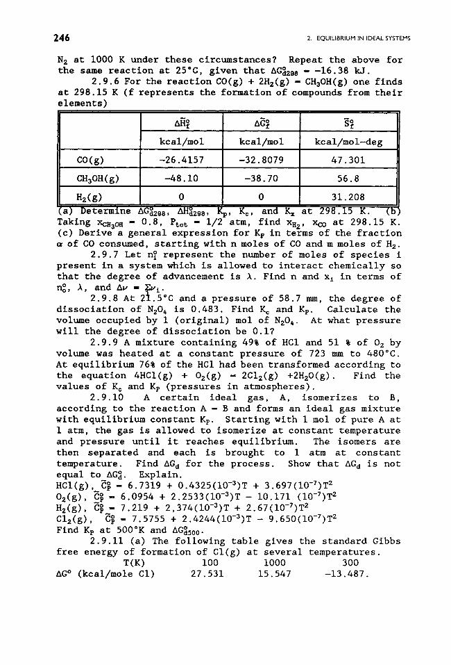
~-~6 2. EQUILIBRIUM IN IDEAL SYSTEMS
N 2 at I000 K under these circumstances? Repeat the above for the same reaction at 25~ given that AG~298--16.38 kJ.
2.9.6 For the reaction CO(g) + 2H2(g ) -CHaOH(g ) one finds at 298.15 K (f represents the formation of compounds from their elements)
, , I , I, , , , , , , , , , , , , , , , , , ,
,, , ,,
CO(g)
CH3OH(g) **
H2(g)
,,,,
kcal/mol
-26.4157
- 4 8 . I0
AG~
kcal/mol
-32.8079
- 3 8 . 7 0
s~
kcal/mol-deg
47.301
56.8
31.208
(a) Determine AG~2~8, AH~298, ~, Ko, and K x at 298.15 K. (b Taking XCH30 H -- 0.8, Ptot - 1/2 aim, find XH2 , Xco at 298.15 K. (c) Derive a general expression for Kp in terms of the fraction of CO consumed, starting with n moles of CO and m moles of H 2.
2.9.7 Let n~ represent the number of moles of species i present in a system which is allowed to interact chemically so that the degree of advancement is A. Find n and x i in terms of n~, A, and Av - ~v i .
2 . 9 . 8 At 2~ .5~ and a p r e s s u r e o f 5 8 . 7 ram, t h e d e g r e e o f d i s s o c i a t i o n o f N204 i s 0 . 4 8 3 . F i n d K= and Kp. C a l c u l a t e t h e volume occupied by i (original) tool of N204. At what pressure will the degree of dissociation be 0.i?
2.9.9 A mixture containing 49~ of HCI and 51 ~ of 02 by volume was heated at a constant pressure of 723 nun to 480~ At equilibrium 76~ of the HCI had been transformed according to the equation 4HCI(g) + O2(g) -2C12(g) +2H20(g). Find the values of K c and Kp (pressures in atmospheres).
2.9.10 A certain ideal gas, A, isomerizes to B, according to the reaction A- B and forms an ideal gas mixture with equilibrium constant Kp. Starting with i mol of pure A at I atm, the gas is allowed to isomerize at constant temperature and pressure until it reaches equilibrium. The isomers are then separated and each is brought to i atm at constant temperature. Find AG d for the process. Show that AG d is not equal to AG~. Explain. HCI(g), C~- 6.7319 + 0.4325(I0-3)T + 3.697(I0-7)T 2 02(g), -C~- 6.0954 + 2.2533(I0-3)T- 10.171 (10-7)T 2 H2(g), C~ - 7.219 + 2,374(I0-3)T + 2.67(I0-7)T 2 Cl2(g) , C~- 7.5755 + 2.4244(I0-3)T- 9.650(I0-7)T 2 Find Kp at 500~ and AG~500.
2.9.11 (a) The following table gives the standard Gibbs free energy of formation of Cl(g) at several temperatures.
T(K) i00 I000 300 AG ~ (kcal/mole CI) 27.531 15.547 -13.487.
CHEMICAL EOUlUBRlUM 247
For the reaction (i/2)C12(g) -el(g), find the equilibrium constant Kp at each of these temperatures. Find the mean AH~ and then find AS~ per unit reaction at each of the temperatures. (b) At 1700~ and i.i0 atm, i g of chlorine occupies 1.96 liters. What are Kp , K x, K c for the reaction (1/2) Cl2(g) -Cl(g)? Assume ideal-gas behavior. (c) At 1600 K, the degree of dissociation of chlorine is 0.071 at i atm. What are Kp, Kx, and Kr for the reaction Cl2(g) - 2Cl(g)? Assume ideal-gas behavior.
2.9.12 (a) At 448~ the degree of dissociation of HI into H 2 and 12 is found to be 0.2198. Determine Kx, Kc, and Kp. (b) If 0.05 tool of H 2 and 0.01 of 12 are brought in contact at that temperature in a volume of 3 liters, what concentration of HI is produced? (c) At 357~ K c - 0.01494; if 0.04 mol of HI, 0.03 tool of 12, and 0.02 tool of H 2 are equilibrated at that temperature in a volume of 3 liters, calculate the composition of the equilibrium mixture in terms of mole fractions, molaritles, and partial pressures.
2.9.13 Let K 1 and K 2 be the equilibrium constants at a temperature T for the reactions 2CO 2 - 2CO + 02 and 2H20 - 2H 2 + 02, respectively. Find K 3 at temperature T for the reaction H 2 + CO 2 - H20 + CO in terms of K I and K 2.
2.9.14 For the reaction 2SO3(g ) - 2SO2(g ) + 02(g ) one finds values of K c - 3.15 x 10 -4 , 3.54 x 10 -3 , and 2.80 x 10 -2 P llter -I at 627, 727, and 832~ respectively. (a) Determine the average enthalpy of reaction under standard conditions in the intervals 627-727~ and 727-832~ (b) Determine K c and Kp at 500, 700, and 1000~ (c) What fraction of SO 3 is dissociated at these temperatures if the total pressure is 2 atm in each case? (d) Assuming air to consist of 79% N 2 and 21% 02 by volume, what percentage of SO 2 is transformed into SO 3 if equal volumes of SO 2 and air are mixed at 727~ at a total pressure of 1 arm?
2.9.15 (a) Derive an expression showing how AS values for a chemical reaction carried out at temperature T I may be related to AS for the same reaction at a different temperature T 2. (b) For the reaction H2(g) + Cl2(g ) - 2HCl(g), the standard entropies at 298 K are 31.208, 53.288, and 44.646 eu/mol for H2(g) , Cl2(g) , and HCI(g), respectively. Also, C~- 6.9409 - 1.999 x 10⁻⁴T + 4.808 x 10-TT 2 cal/deg-mole (H2) C~- 7.5755 + 2.4244 x 10⁻³T- 9.650 x 10⁻⁷T 2 cal/deg-mole (C12) ~0_ 6.7319 + 0.4325 x 10⁻³T + 3.697 x 10-TT 2 cal/deg-mole (HCI)
Calculate AS~ at 298 and 1200 K for these reactions. 2.9.16 (a) Find K for H2(g ) + 12(g ) - 2Hl(g); AG~98 =-4.01
kcal. (b) Find Kp for 2Hl(g) - H2(g) + 12(g ). (c) Find Kp for
(I/2)H2(g) + (1/2) 12(g)- HI(g). (d) For H2(g) + 12(g) - O 2Hl(g), Kp - 870 at 298 K and AHd2s8 - -2.48 kcal. Find Kp at
328 K, assuming AH d is constant in this temperature range.
~-48 2. EQUILIBRIUM IN IDEAL SYSTEMS
2.10 CHEMICAL EQUILIBRIUM IN HOMOGENEOUS IDEAL SOLUTIONS
(a) The methodology of the preceding section will now be
applied to homogeneous ideal solutions which form condensed
phases. Here Eq. (2.5.1) is applicable, ~I(T,P) -~(T,P) + RT
In xl, where ~i is the chemical potential of pure i, i.e., the
value obtained when x i - x~ - i. The equilibrium condition now
reads
0- ( vi~i).q- vi~i(T,P) + RT ( v i ~n xl).q. (2.1o.i)
Again, it is convenient to define an equilibrium 'constant' as
follows"
2n K.-- ~ vllm~(T,P)/RT- (~ w, In x,).q. (2.10.2)
This has the same form as Eq. (2.9.5a) except that in the
present case K Z depends parametrically on T and P. Accordingly,
by the method of Section 2.9,
(a2n K./aT)p - vIHI(T,P)/RT 2 - AH$/RT 2
(a~n K./aP)T - - vIVI(T,P)/RT - - AV$/RT,
and, by analogy with Eqs. (2.9.8),
(2.10.3)
(2.20.4)
AG d -- RT 2n K x + RT ~ v i 2n x i (2.10.5a)
- AG~* + RT ~ w i 2n x i. (2.10.5b)
(b) Since equilibrium constants in solutions are
frequently expressed in terms of concentration units such as
molallty m i or molarity cl, it is necessary to examine the
relation between xl, ml, and c i. From the definition of
molarlty and mole fraction we obtain
cl/x i - (nl/VL) (~nj/nl), v L - V/lO00, (2.10.6)
HOMOGENEOUS IDEAL SOLUTIONS 249
where V is the volume of the solution in cm 3. The latter
quantity is related to the density p of the solution by V-
ms/p, and the mass of the solution is given by m s - Y.(j)njMj,
where Mj is the gram atomic mass of constituent J. Thus,
i0009(i + n~/nz + ns/nz +...) ci/x i - I0000~ nj/~ njMj -
M I + (n2/nz)M2 + (na/nz)M3 +...
(2.10.7)
Consider now the case of a dilute solution for which one can
sensibly expect near-ideal behavior. Let the subscript I
designate the solvent. Then Eq. (2.10.7) reduces to (for
niMi/n I << Mz, n• I << I)
cl/x i : 1000#z/Mz. (2.10.8)
In llke manner, the definition of molallty leads to the
relation
milx i _ (nil0001nlM1)(~ njlni) - (10001nlMl) ~ nj - 10001xiM I, J J (2.10.9)
where the subscript I again refers to the solvent. For dilute
solutions,
ml/x i - (1000/nxMz)nl( I + n2/n I + na/n I + ...) = 1000/MI.
(2.10.10)
We then see that for a solution which is ideal
2n K e - (~ v i Sn cl).q - 2n K x + ~ v i 2n [1000p~. nj/~ njMj],
z 3 3 (2. I0. lla)
giving rise to the expression
Ko - ~ (cl "i).q. (2.10.11b)
Furthermore, we find
2n ~- (~ vl 2n ml),q - 2n K x + ~ v i 2n [1000/MIx1], (2.10.12a) 1
2~0 2. EQUILIBRIUM IN IDEAL SYSTEMS
giving rise to the expression
~. _ [~ (ml ~i ).q. (2.10.12b)
For a solution that is ideal only when dilute, the
arguments of the last logarithmic term on the right of Eqs.
(2.10.11a) and (2.10.12a) may be replaced by 1000pl/M I and
1000/MI, respectively. Finally,
AG d - - RT 2n K c + RT ~ u i 2n c i - AG~ c + RT ~ w i 2n c i l l
(2.10.13)
AG d - - RT 2n K m + RT ~ v i 2n m i - AG~ m + RT ~ v i 2n m i.
i (2.10.14)
It should also be evident that
d2n K x - d2n K m - d2n K= - (~ v l)d2n p. (2.10.z5)
This latter relation readily permits the analogues of Eqs.
(2.10.3) and (2.10.4) to be written down.
(c) Once more, the remarks of the preceding section on
AGd, AG~, AH~ are invoked here. One must satisfy the conditions
of" (a) Constant T, P, (b) infinitesimal, reversible
advancement, and (c) maintenance of standard states where
appropriate. Confusion with integral changes in AG or AH is
best avoided by reverting to the definitions AG~ x -
Z(1)vi~i(T,P), AH~ x- E(1)viH~(T,P). For molarity or molality, the
reference states clearly require that c i ~ 1 and m i = I,
respectively. When mole fractions are used the reference state
is x~ - I. For this latter case, one seems to run into the
apparent contradiction of having to determine AG~ x and AH~ x
while carrying out the reaction Y.(1)wiAi - 0 with all
participating species in pure form, i.e., completely isolated
from each other. This problem is to be resolved in Exercise
2.10.1.
One other item is noteworthy" Because of the definitions
adopted here, Kx, Kc, and K W differ from one another, although
HOMOGENEOUS IDEAL SOLUTIONS 251
they refer to one and the same system. In Section 7(b) of
Chapter 3 we provide a self-consistent set of definitions that
involve but a single equilibrium constant. It will also be
shown how one single quantity is related to the above
equilibrium constants. In Section 3.9 the quantities Kc, K m
defined by Eqs. (2.10.11a) and (2.10.12a) are derived as
special cases of a more general approach.
(d) The specification of equilibrium constants certainly
is not unique. This may best be seen by referring back to Eqs.
(2.5.14)-(2.5.16), in which the chemical potentials are
specified relative to standard chemical potentials (with P =
i). For example, when dealing with mole fractions, one writes
pi(T,p,xl) = ui(T,l,x~) + RT 2n x i. The reader should be able
to verify that in place of Eq. (2.10.2) one would then have
been led to introduce an equilibrium *constant' K x by the
relation
2n K x m- (I/RT) vlpi(T,l) = ( v i 2n xl),q , l
which leads to the expression
( 2 . 1 0 . 1 6 )
(2.10.17)
As a consequence the quantity AH~ x in Eq. (2.10.3) must be
replaced by AH~ x, which now refers to the summation Y.(i)viHi(T, I)
for an infinitesimal advancement of the reaction Y.(i)viAi--0,
with all constituents in their standard state. We thus obtain
d 2 n K x = AH~ x dT R--~-'z �9 ( 2 . 1 0 . 1 8 )
Clearly (8~n Kx/aP) T = 0. The analogue of Eqs. (2.9.8) becomes
AG d - ~ v i#~(T,l) + RT .~ v i 2n x i = AG~ x + RT ~. v i ~n x• l 1 1
= - RT ~n K x + RT ~ v i 2n El, T l
( 2 . 1 0 . 1 9 )
~-5~- 2. EQUILIBRIUM IN IDEAL SYSTEMS
where AG~* now refers to the differential free energy change for
the reaction Y'(1) ViAl- 0 under standard conditions.
In a similar vein, from Eq. (2.5.16) one obtains the
equilibrium condition (Y.(1)vi~i),q- 0 in the form
0- ui~i(T,l) + RT( w i 2n ci(T,P)),q - RT ~ v i ~n c~(T,l),
z (2.10.20)
which suggests the following definition of an equilibrium
constant K c
2n K c = - (I/RT) ui~ i(T,l) - u i 2n c•
- (~ u i 2n cl).q, (2.10.20a)
where K c is related to a rather more complex set of parameters
than is K c. As is obvious, K c does not depend on pressure.
With this definition the relationship analogous to Eq.
(2.10.17) can be written down as
Furthermore,
(2.10.20b)
AG d - vi~i(T,l ) + RT v i 2n ci(T,P ) - RT v i ~n ci(T,l)
- AG~ c + RT ~ v i 2n ci(T,P) -- RT In K c i
+ RT ~ v i 2n ci(T,P). I
(2.10.21)
By strict analogy one obtains a third equilibrium
constant related to molality in the form
2n K m - - (I/RT) wi~zi(T,l ) - w i ~n m i = ( w i 2n ml)eq ,
z (2. i0.22a)
so that
K. - ~ (ml ~i).q. (2. i0.22b)
HOMOGENEOUS IDEAL SOLUTIONS 2S 3
Also,
AG d - vi~ i(T,l) + RT v i ~n m i - RT v i ~n m i
- AG~ + RT ~ v i 2n m i -- RT 2n K= + RT ~ v i 2n m i. l l
(2.10.23)
It is customary to work with the equilibrium constants Kx,
Kc, K m that are related to standard conditions, i.e., to
standard rather than reference chemical potentials. Then the
superscripts in AG~ x, AG~ c, AG~ refer to the differential Gibbs
free energy changes accompanying the reaction Z(i)wiA i -0 in
which all constituents are maintained under standard
conditions. The fact that actual reactions cannot often be
carried out under such circumstances is no deterrent: The
principal point of practical interest is that products of the
type ll(x i ).q etc., are constant at fixed temperature. The
partlclular value of the constant can then be deduced by
consulting tables of numerical values of free energies for all
constituents i that are involved in the chemical reaction
Z(1)viAi -0; such listings are invariably provided in terms of
standard conditions. Thus, although definitions of the type
(2.10.2), (2,10,11a) or (2.10.12a) for K., K c, K m are perfectly
satisfactory they are not as useful as the definitions
(2. I0.16a), (2. I0.20a) or (2. i0.22a) for Kx, Kc, K m,
respectively. This discussion points to the fact that
equilibrium constants are not of fundamental importance in
themselves; it is only the quantities AGd for a given reaction
that are unique. The reader is referred to the illustration in
Chapter 3 that makes these matters more explicit.
The above arguments do not, however, however, detract
from the utility of the concept of equilibrium 'constants':
Consider the relationships
Kq- exp(- A~q/RT) and Kq- exp(- AGSq/RT), (2.10.24)
with q - x,c,m. If Kq or Kq is numerically very large and
positive, then AG~q or AG~q must be large and negative; that is,
~ 4 2. EQUILIBRIUM IN IDEAL SYSTEMS
the corresponding reactions Y.(1)uiAi - 0 carried out under
appropriate conditions must proceed in the direction as
written. The equilibrium shifts to the right, so that products
predominate over reagents. Conversely, for extremely small
numerical values of Kq or Kq the corresponding AG~ q or AG~ q will
be large, positive numbers; the reaction characterized by these
quantities will then proceed in the opposite direction.
Equilibrium conditions then establish a preponderance of
reagents over products for the reaction as written. Clearly,
numerical values of Kq or Kq close to unity represent cases
where reagents and products are equilibrated at roughly similar
concentrations.
EXERCISES
2.10.i Devise schemes (preferably practical ones, but otherwise, schemes that are at least conceptually possible) for determining AG~ and AH~ for a reaction which is carried out with all reagents in their isolated, pure states under standard conditions.
2.10.2 (a) For the reaction C5HI0(~ ) + CH3COOH(2 ) - CH3COOCsH11(2), start with _a moles of pentene and b moles of acetic acid; m moles of CH3COOCsH11 are present when equilibrium is reached. Express K x and K= in terms of a, b, _c, V. (b) Repeat, under the assumption that n moles of an inert solvent are also present.
2.10.3 For the reaction C5H10 + CCI3COOH - CC13COOC5H11 , one finds that at IO0~ 2.15 tool of amylene and i tool of the acid react to yield 0.702 tool of the ester at equilibrium. What fraction of the acid will be used in ester formation when 3.00 and 7.00 mol of amylene and acid are used in the starting mixture at IO0~
2.11 CHEMICAL EQUILIBRIUM IN IDEAL HETEROGENEOUS SYSTEMS
We now provide a preliminary discussion of chemical equilibrium
in ideal heterogeneous systems. This treatment is provisional
since the generalized approach of Section 7 of Chapter 3 is
more systematic and does not require a distinction to be made
IDEAL HETEROGENEOUS SYSTEMS 2 ~
between pure condensed phases and dissolved species. In
Chapter 3 we shall show how final results such as Eq. (2.11.13)
are derived as special cases from the more general
relationships of Sections 3.7 and 3.9.
(a) Consider chemical reactions in heterogeneous systems
where one or more pure condensed phases coexist with ideal
homogeneous mixtures (gases, liquid solutions, or solid
solutions). In an extension of the previous scheme we
symbolize such a chemical reaction by 7. usA s + ~ uiA i -- 0, where
s refers to pure condensed phases and i, to the components of
various mixtures. As before, w i and w, represent stoichiometry
coefficients. Equilibrium is now characterized by the
condition
ACd - (~ v , # , ) oq + I ~.~ . o . (2.11.1) s
(b) For ideal gaseous mixtures in equilibrium with a pure
condensed phase,
vi#~(T) + 7. vs#,(T,P) + RT( vl ~n Pi).q s
- O, (2.11.2)
where ~(T) - ~P(T). It is now convenient to define an
equilibrium ~constant' by
~n K p - - (1/RT) v~.~(T) + ~ v . . . ( T , P ) , ( 2 . 1 1 . 3 ) s
so that Eq. (2.11.2) may be rewritten as
2n Kp - (~ v i ,~n Pi)eq; Kp - ~ (P~i)eq. (2.11.4a)
Once more we have hereby separated quantities depending on T
and total pressure P from quantities depending on the
composition of the gas phase. One should note that the
definition (2.11.3) includes all terms referring to the pure
condensed phases. As a result, the equilibrium constant as
2 S 6 2.. EQUILIBRIUM IN IDEAL SYSTEMS
specified by (2.11.4a) involves only the partial pressures of
the gases. In some texts one finds statements to the effect
that pure condensed phases are at "unit activity" and that for
this reason concentration terms on the right-hand side of
(2.11.4a) referring to such phases are lacking. In actuality,
Eq. (2.11.4a) comes about because of the manner in which Kp has
been defined, this definition being strongly suggested by the
structure of Eq. (2.11.2).
Analogous to (2.11.4a) one also obtains, for an ideal gas
in equilibrium with condensed phases, the relations
2 n K c - ( ~ v i 2 n c i ) , q (2. ll.4b)
~n K x - (~ vl ~n x i),q. (2.11.4c)
Note that the summation involves solely the species in the gas
phase. On account of the expression Pi - ciRT - xIP the various
equilibrium ~constants' are interrelated by
2n Kp - 2n K o + ~ v i 2n RT - 2n K x + ~ vl 2n P. (2.11.5)
One must note that the above equilibrium 'constants' all depend
parametrically both on T and on P. In fact,
(a2n Kp/OP)~ . . . . (82n Kc/OP) T - (I/RT)~ vs(ap*s/aP)T ~ vsVs/RT-* S S
- - AV:/RT. (2. ii. 6)
Only the terms referring to the condensed phases appear on the
rlght-hand side of (2.11.6), since p~ does not depend on P.
Normally, the partial molal volume changes of the pure
condensed phases during the chemical reaction are very small;
hence, the rlght-hand side is close to zero. By contrast,
(82n l(x/SP)~ - - ~ vl/P + (Sfn Kp/SP)T
- v,V,/RT - (AV~/RT) S
(2.11.7)
IDEAL HETEROGENEOUS SYSTEMS 25 7
involves the total volume change of all species, when isolated,
in the chemical reaction.
Further,
(a~n Kp/0T)p- (a2n K=/aT)p- wiH~ + 7. v,H, /RT z - AH~/RT z s
(2.11.8)
which encompasses both condensed and gaseous species on the
right. On the other hand,
(82n Kc/ST)p - (a2n Kp/ST)p - ~ vl/T - [AH~ - ~ vIRT]/RT z, (2.11.9)
where the summations on the right involve only the gaseous
species. Finally,
AG4 -- ~. vi#~ + ~ v,#,+ RT ~ v i 2n Pi - AG~ + RT ~ wi 2n Pi s i
-- RT 2n Kp + RT ~ w i 2n P i (2.11.10a)
- - RT 2n K= + RT ~ v i ~n c i (2.11.10b)
- - RT ~n K x + RT ~ v i ~n x i. (2.11.I0c)
(c) For ideal solutions in equilibrium with pure
condensed phases, we can write again
AG d - wi#i(T,P ) + ~ w,#,(T,P) + RT (~ u i ~n xl)eq s 1
*x
- AG d + RT (~ wl 2n x i),q - 0. (2.11.ii)
Here the ~I(T,P) are the reference chemical potentials for all
components i in pure form which make up the homogeneous
solution, whereas the #, refer to the chemical potentials of the
pure condensed phases. We proceed as before by defining
2n K x - - (I/RT) v,#, + ~ vi# i - - AGa/RT, (2.11.12)
'~.~8 2. EQUILIBRIUM IN IDEAL SYSTEMS
so that
.~n K x - (~ u i ,en x i ) eq ; K x - ~ (xlVl)eq, (2.11.13)
which may be compared with (2.11.4c); obviously, the x i here
refer to mole fractions of various components dissolved in
solution.
The subsequent analysis proceeds as before. In
particular, Eqs. (2.11.7) and (2.11.8) hold for the variation
of 2n K x with P and T. Furthermore, one may define a set of
equilibrium constants K= and K s or K= and Kin, just as in Sec.
2.10, with corresponding interrelations; these matters are left
as a problem in Exercise 2.11.2. Again, a much more systematic
approach to this problem is provided in Section 7 of Chapter 3.
EXERCISES
2.11.1 Derive expressions showing how 2n K x changes with temperature and pressure.
2. II. 2 By analogy to Section 2. I0, write down expressions for K= and K s for the case considered in this section and show by analytic expressions how K= and K s change with T and P. Repeat for Kx, Kc, and K m.
2.11.3 (a) Write down a general expression for AS d for a chemical reaction in terms of partial molar entropies of the participating species. (b) For the reaction 2C(s) + 4H2(g ) + Oz(g ) - 2CHsOH(2), the molar values of the entropy in eu under atmospheric conditions at 298 K are 1.372 for graphite, 31. 208 for hydrogen, 49. 003 for oxygen, and 30.3 for methanol. Determine AS~ for the reaction. (c) Explain the large negative value that is found.
2.11.4 (a) The dissociation pressures reported for CaCO s are 372, 760, 793, 1577, 2942 mm at 850, 897, 900, 950, 1000~ respectively. Determine the enthalpy of transition at 9250C. (b) Compare this result wlth the calculation based on the empirical equation log P(mm Hg) i-II.355/T- 5.388 log T + 29. 119. (c) Determine AG~, AH~, AS~ for the reaction.
2.11.5 In the temperature range 50-II0~ the vapor pressure of Br2(g) over CuBr 2 is given by log P(mm Hg) = 5056/T + 12.01. Obtain AG~, AH~, AS~ at 250C for the reaction 2CuBr2(s ) - 2CuBr(s) + Br2(g).
2.11.6 For the reaction B4C(s ) - 4B(g) + C(s), the equilibrium vapor pressure in the temperature range 2350-2615
IDEAL HETEROGENEOUS SYSTEMS 2 5 9
K is given by log P(atm) - 7.506 - 29.630/T. (a) What is the equilibrium constant at 2350 K? (b) What is the equilibrium constant at 2350 K for the reaction (I/4)B4C(s) - B(g) +(i/4)C(s)? (c) 5 g of B4C are enclosed in a i0 cc crucible and equilibrated at 2350 K. What are the equilibrium numbers of moles of B4C , C, and B in the system? The density of B4C is 2.5 g/cc. (d) 1.0 x 10 -I~ tool of B gas is added to the system described in (c). What is the equilibrium pressure of B and what are the mole numbers of B4C , C, and B at equilibrium? (e) 4.29 x 10 -I~ tool of B gas is added to the system described in (c). What is the equilibrium pressure of B and what are the mole numbers of B4C and of B at equilibrium? (f) 5 x 10 -I~ mole of Ar is added to the system described in (c). What is the total pressure of the system at equilibrium? What are the mole numbers of all components of the system at equilibrium?
2.11.7 For the reaction ZnO(s) + CO2(s) - ZnCO3(s) carried out at constant volume, AF --3.91 and AE --16.4 kcal/mol at 298 K. AE is nearly independent of T. (a) At what temperature is equilibrium reached when the gas pressure is i atm? (b) What is the entropy change AS a under these conditions?
2.11.8 For the reaction NiO(s) -Ni(s) + (I/2)O2(g), appropriate tabulations lead to a value of AG~29s - 211.7 kJ/mol. Determine the partial pressure of oxygen in equilibrium with NiO(s) at 25~ Note and comment on the magnitude of the numerical value.
2.11.9 The AG~ 298 values of formation of NH4CI(s), NHs(g), and HCI(g) from their elements are-48.51, -3.94, and 22.777 kcal/mol respectively. Determine the partial pressure of HCI vapor over NH4CI(s) at 25 ~
2. ii. i0 When H2NCOONH 4(s) is introduced into an evacuated vessel at 30~ the total pressure resulting from the attainment of equilibrium is found to be 125 ram. Find K~ for the process HzNCOONH4(s) - 2NH3(g ) + C02(g).
2.11.11 Consider the reaction 3MnzO3(s) - 2Mn304(s) + (I/2)02(g) . Utilizing the data tabulated below, estimate the temperature at which the equilibrium pressure of 02(g) over the two manganese oxide phases is 0.20 atm. State any assumptions that you make.
Species
Oa(g)
Mna03 ( s )
Mn304 ( S )
AG~(298 K, kcal tool -I)
-212.3
-306.0
S~ K, cal deg-lmol -I)
49.0
22.1
35.5
2 6 0 2. EQU,L, BR,UM ,N ,OEAL SYSTEMS
2.11.12 For the reaction CaC0s(s) - CaO(s) + CO2(g), the dissociation pressure in at is given by log(Pco2) --II.355/T - 5.88 log T + 26.238. Determine AH~ for the reaction as a function of T.
2.12 EQUILIBRIUM INVOLVING IDEAL MIXTURES IN TWO PHASES
(a) One of the important applications of equilibrium
constraints occurs in cases where an ideal was mixture is in
equilibrium with an ideal liquid solution. From the constraint �9 N
#I(T,P) -~I(T,P) for each component i in the two phases denoted
by the accents, one flnds that
* , " ~ c " ~i(T P) + RT 2n xl - ~P(T) + RT 2n Pi - (T) + RT 2n c i
N
_ ~X(T,p) + RT 2n x i, (2.12.1)
where the left refers to the liquid, and the right, to the gas.
Obviously, six more relations could have been written out,
wherein the concentrations for the liquid phase occur in terms
of molarlty and molallty, but we shall not pursue all the
consequences of such an approach.
On introducing appropriate equilibrium constants ~n Kex -
-[~P(T) - ~I(T,P)]/RT, etc., one can reformulate the above
equilibrium constraint as
K~ - P[/xl; Kcx - c[/xl; Kxx - x[/xl, (2.12.2)
N N ~ �9
where equilibrium values of Pi, cl, xl, xl are to be used. w �9 �9
Since for dilute solutions x i = (lO00p1/M1)c I = (1000/M1)m I the
various constants may be absorbed in the equilibrium constants,
so that one obtains
Kp= - P[/c[; K== - c[/c[; K~= - x[/c'i; Km - P[/m~; ap N �9
K=~- c l/ml; K~- xl/ml. (2.12.3)
One should note the following" The relation Kpx- P[/xl is
simply a reformulation of Raoult's Law when applied to the
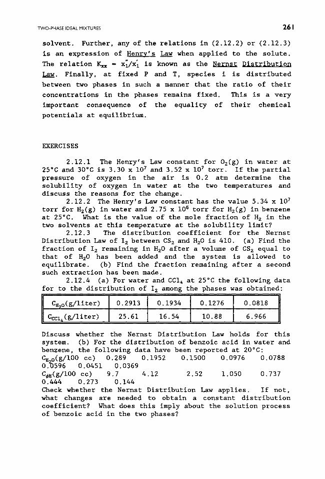
TWO-PHASE IDEAL MIXTURES 2 6 I
solvent. Further, any of the relations in (2.12.2) or (2.12.3)
is an expression of Henry's Law. when applied to the solute.
The relation K~x- x[/xl is known as the Nernst Distribution
Law. Finally, at fixed P and T, species i is distributed
between two phases in such a manner that the ratio of their
concentrations in the phases remains fixed. This is a very
important consequence of the equality of their chemical
potentials at equilibrium.
EXERCISES
2.12.1 The Henry's Law constant for O2(g) in water at 25~ and 30~ is 3.30 x 10⁷ and 3.52 x 10⁷ torr. If the partial pressure of oxygen in the air is 0.2 atm determine the solubility of oxygen in water at the two temperatures and discuss the reasons for the change.
2.12.2 The Henry's Law constant has the value 5.34 x 10⁷ torr for H2(g) in water and 2.75 x i0 s torr for H2(g ) in benzene at 25~ What is the value of the mole fraction of H 2 in the two solvents at this temperature at the solubility limit?
2.12.3 The distribution coefficient for the Nernst Distribution Law of I 2 between CS 2 and H20 is 410. (a) Find the fraction of 12 remaining in H20 after a volume of CS 2 equal to that of H20 has been added and the system is allowed to equilibrate. (b) Find the fraction remaining after a second such extraction has been made.
2.12.4 (a) For water and CCI 4 at 25~ the following data for to the distribution of 12 among the phases was obtained"
, . . . . . . . . . . . . . , . . . . . .
CH2o(g/liter ) 0. 2913 0. 1934 0. 1276 0.0818
Cccl~(g/liter) 25.61 16.54 I0.88 6. 966 :,~ . . . . .. ,.j
Discuss whether the Nernst Distribution Law holds for this system. (b) For the distribution of benzoic acid in water and benzene, the following data have been reported at 20~ C~_o(g/lO0 cc) 0.289 0.1952 0.1500 0.0976 0.0788 0.~596 0.0451 0.0369 C~H(g/100 cc) 9.7 4.12 2.52 1.050 0.737 0.444 O. 273 O. 144 Check whether the Nernst Distribution Law applies. If not, what changes are needed to obtain a constant distribution coefficient? What does this imply about the solution process of benzoic acid in the two phases?
2 6 2 2. EQUILIBRIUM IN IDEAL SYSTEMS
2.12.5 Pure water is saturated with air at I0 atm pressure�9 Calculate the molar ratio xN : x o in water Assume air to be a 4 i tool mixture of N 2 and 202 2 �9 and take the Henry's Law constant for N 2 and 02 to be 8.74 x 10⁴ atm and 4.59 x 10⁴ atm, respectively.
2.13 ENTROPY PRODUCTION DURING IRREVERSIBLE PROCESSES
All actual processes, even if carried out slowly in
quasistatic steps, are irreversible. As long as departures
from equilibrium are slight one can assign average uniform
values to all properties of the system at each step as the
system progresses through all intermediate states. The values
assigned at any stage are those which the system would assume
if it were suddenly adiabatically insulated and allowed to come
to equilibrium. On the other hand, if departures from
equilibrium become too severe for the above procedure to apply,
the continuum methodology of chapter 6 must be employed.
We base our present development on the discussion of
Section 1.16 where a distinction was made between the entropy
change of a system dS - ~Q=/T, associated with the reversible
transfer of heat across the boundaries, and the entropy change
arising from irreversible processes occurring totally within
the system. As shown in Section 1.15, the heat transfer is
subject to the relation ~Q _< TdS; whenever the inequality sign
applies, one introduces the deficit entropy function 8 so as to
render
~Q- T dS - T~8 (~8 >_ 0). (2.13.1)
The First Law of Thermodynamics then becomes
dE - T dS - T~8 - ~YW. (2.13.2)
One may now distinguish between (i) an adiabatic process
wherein ~Q - 0; then the entropy of the system increases
according to dS- ~8, reflecting the occurrence of irreversible
processes within the system; and (ii) an isentropic process, in
ENTROPY PRODUCTION DURING IRREVERSIBLE PROCESSES ~6
which dS - ~e - 0, as a result of which dE -- ~W. Thus, only
reversible adiabatic processes are also isentroplc.
A trivial rearrangement of Eq. (2.13.1) leads to the
relation
dS -- ~Q/T + ~e, (2.13.3)
which can readily be reformulated as a rate law
- Q/T + ~t (8 >_ 0 ) , (2.13.4)
showing that the rate of production of entropy in an
irreversible process is governed by two factors: (i) the rate
of heat transport Q across the boundaries, corresponding to an
entropy flux Q/T into the system (Q/T < 0 if there is a net
flow out of the system); (il) the rate of production of entropy
through irreversible processes, usually arising from
processes occurring totally within the system. The latter
claim may be illustrated by comparing Eq. (2.13.2) with the
First Law formulation for open systems, yielding
dE - ~Q + T~8 - ~W + ~ ~idnl, (2.13.5)
so that if no work is performed and if the system is isolated,
~8 - - ~ (~i/T)dn i (2.13.6)
as the entropy change occurring due to changes in composition
via reactions that occur totally within the isolated system.
Equation (2.13.6) at first glance seems to contradict (1.24.4).
However, it must be remembered that Z ~idnl - 0 only when i
equilibrium prevails, a matter already emphasized in Section
1.24. Here we are considering the reactions for which the
foregoing constraint does not apply; i.e., the concentration of
all species may be altered not only by transfer of matter
across the system boundaries, but also by reactions occurring
totally inside the system.
~-64 2. EQUILIBRIUM IN IDEAL SYSTEMS
2.14 ENTROPY AND IRREVERSIBILITY IN CHEMICAL REACTIONS : THE
CHEMICAL AFFINITY
For an open system undergoing a chemical reaction the first law
of thermodynamics may be written as dE - TdS - pdV + Z(1)vi~idA,
where the index i runs over all of the species participating in
the chemical reaction E(1)wiA i -0, and where A is the degree of
advancement of the reaction.
We now recall the argument of Section 2.13, according to
which the entropy produced during an irreversible process (in
this case, a chemical reaction) is given by ~O - -~(j)#jdnj/T.
Accordingly, we can now write for the chemical process under
consideration
~O - -T -I ~ vi#idA. (2.14.1)
It is convenient to relabel the quantity- Z(1)vlpl with
the symbol A, termed the chem$ca! affin.$ty by de Donder (1923).
Then the rate of entropy production associated with the
irreversible processes in the chemical reaction Z(1)viA • -0 is
given by
- (A/T) (dA/dt), (2.14.2)
where dA/dt is the rate of the chemical reaction. Again, as in
Section 2.2, Eq. (2.14.2) admits of the interpretation whereby
A/T is a generalized force F and dA/dt is a flux- here, the
rate of a reaction, involving chemical species within the
system. As in Section 2.2 we write 0 - ~(1)FiJi.
The four fundamental thermodynamic relations may now be
cast in the form
dE - TdS - PdV - Adl, dF - - SdT - PdV - Adl,
d H - T d S + V d P - A d A , dG -- SdT + VdP - AdA. (2.14.3)
Further, since in any natural process the entropy production
ENTROPY AND IRREVERSIBILITY IN CHEMICAL REACTIONS ~6~
rate must be positive we find that (A/T)(dA/dt) > 0. Then for
A > 0, Z(1)vi~ i < 0 and thus dA/dt > 0, whereas for A < 0,
Z(i)vi~ i > 0 and dA/dt < 0. The chemical reaction as written
thus proceeds to the right or to the left depending on the sign
of the corresponding affinity. Equilibrium is attained when A
- 0, i.e., when Z(1)vi~ i - 0, at which point dA/dt - 0. We have
previously recognized the relation Z(1)vi~ i -0 as corresponding
to the equilibrium state. The quantity- Z(1)vi~ i -A is
frequently used in the treatment of irreversible phenomena,
beginning with Section 6.2. However, in the present context
such a designation tends to hide the thermodynamic
significance of the differential quantity Z(1)v• i - AG d which is
to be carefully distinguished from the difference AG w
Z(1) (ni~i)~In,l - Z(1) (ni~i) inlti,:"
The generalization to several simultaneous reactions may
be readily accomplished. Every reaction r is specified by its
own degree of advancement dA r and the various chemical reactions
Z(i)wi=Air - 0 are characterized by affinities of the type A r -
- Z(i)wlr~i (note that the subscript r is missing from ~: why?).
The total rate of production of entropy due to all chemical
reactions running irreversibly and simultaneously is then
- (I/T)~ Ar(dAr/dt). (2.14.4) r
At equilibrium one has 8 - 0, and this can be guaranteed only
by having A r - 0 or Z(1)Vlr# i - 0 for each reaction separately.
Clearly, Eq. (2.14.3) must be rewritten so that AdA is now
replaced by Z(r)ArdA r.
EXERCISES
2.14.1 Show how the affinity A may be specified in terms of the four thermodynamic functions of state.
2.14.2 By Maxwell-type relationships, establish equations linking A to T, S, P, and V. Discuss possible uses of these relationships.
Recommended