Estimating and Accounting for the Output Gapwith Large Bayesian Vector Autoregressions
James Morley1 Benjamin Wong2
1University of Sydney
2Reserve Bank of New Zealand
The view do not necessarily represent those of the Reserve Bank of New Zealand
ASSA Annual Meeting, Philadelphia, PA5-7 January 2018

Introduction
I Most T-C methods are univariate (e.g. HP filter, Bandpass filter,Watson (1986) UC model etc)
I Beveridge-Nelson (BN) decomposition is a natural way toincorporate multivariate information (e.g. Evans and Reichlin, 1994)
τt = limj→∞
Et [yt+j − j · E [∆y ]]

Estimated U.S. Output Gap from Univariate andMultivariate BN Decompositions (% Dev from trend)
2 variable VAR includes output growth and the unemployment rate. 3 variable VAR includes output growth, CPI inflation, and the federal
funds rate. 7 variable VAR includes all of the variables in the 2 and 3 variable systems, as well as capacity utilization, the growth of
industrial production, and the growth of real personal consumption expenditure.


Punchlines
Contribution
1. Show how to incorporate multivariate information into trend-cycledecomposition
I Requires only large standard BVARs ala “Minnesota with a twist”
2. Show how to interpret trend-cycle decomposition through theincluded multivariate information
Main Findings
I BVARs with up to 138 variables produce plausible/intuitiveestimates of the U.S. output gap
I Unemployment rate, CPI, housing starts, consumption, stock prices,real M1, and federal funds rate are key informational variables
I Estimates largely robust to including additional variables
I Monetary policy shocks play little role in the output gap, while oilprice shocks explain about 10% of variance over different horizons
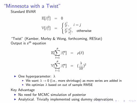
“Minnesota with a Twist”Standard BVAR
E[βijl ] = 0
V[βijl ] =
{λ2
l2 , i = jλ2
l2σ2i
σ2j, otherwise
“Twist” (Kamber, Morley & Wong, forthcoming, REStat)Output is sth equation
E[
p∑l=1
βssl ] = ρ(δ)
V[
p∑l=1
βssl ] = (
λ
10)2
I One hyperparameter: λI We want λ → 0 (i.e., more shrinkage) as more series are added inI We optimize λ based on out of sample RMSE
Key AdvantageI No need for MCMC simulation of posteriorI Analytical. Trivially implemented using dummy observations

U.S. Output Gap (BN Filter aka Wellington Prior), δ̄ =0.25 (Kamber, Morley & Wong, REStat, forthcoming)
Data
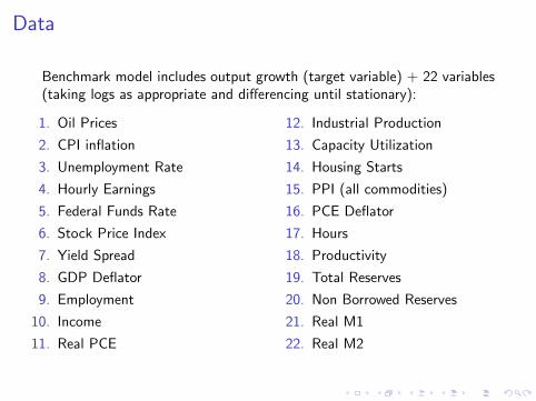
Benchmark model includes output growth (target variable) + 22 variables(taking logs as appropriate and differencing until stationary):
1. Oil Prices
2. CPI inflation
3. Unemployment Rate
4. Hourly Earnings
5. Federal Funds Rate
6. Stock Price Index
7. Yield Spread
8. GDP Deflator
9. Employment
10. Income
11. Real PCE
12. Industrial Production
13. Capacity Utilization
14. Housing Starts
15. PPI (all commodities)
16. PCE Deflator
17. Hours
18. Productivity
19. Total Reserves
20. Non Borrowed Reserves
21. Real M1
22. Real M2

U.S. Output Gap (Benchmark Model, % Dev from trend)

Trend and Cycle can be written as a linear decompositionof all the historical forecast errors
Consider companion form of VAR(p) forecasting model:
(∆xt − µ) = F(∆xt−1 − µ) +Hνt
Let Γi = Fi(I − F)−1
, BN decomposition implies
ct ≈ −
{t−1∑i=0
Γi+1Hνt−i
}∆τt = µ + Γ0Hνt .
Two Decompositions
1. Sources of informationI Which variables contain the most information for estimating trend
and cycle?I Which variables should be included in forecasting model?
2. Role of Structural ShocksI Given forecast errors and identification restrictions, SVAR analysis
straightforwardI What drives the trend and cycle?

Historical Decomposition of Role of Forecast Errors(Benchmark Model)

Historical Decomposition of Role of Forecast Errors(Benchmark Model)
Historical Decomposition of Role of Forecast Errors(Benchmark Model)

Standard Deviations of Informational Contributions

Varying the Information Set (% Dev from trend)

Omitting Important Information (% Dev from trend)

Out of Sample RMSE (one-step ahead, real GDP growth)

Causal Determinants of Output Gap and Trend Growth
I We identify two shocks using standard timing restrictionsI An oil price shockI A monetary policy shock
I Then we consider a forecast error variance decomposition (FEVD)and a historical decomposition

Variance Shares (%)

Historical Decomposition (% Dev from trend)

Summary
I Bayesian shrinkage makes application of BN decomposition withlarge information sets feasible and avoids overfitting
I Movements in trend and cycle can be accounted for based ondifferent sources of information or structural shocks
I When estimating the U.S. output gap, it is more important toinclude key variables than to consider a really large information set(i.e. unemployment)

Other Applications and Extensions
Work-in-Progress
I Global Influences of Trend Inflation (Kamber and Wong, 2018, BISworking paper)
I Role of foreign shocks in driving output gap and trend growth foropen economies (Morley, Vehbi, and Wong, in progress)
Pipeline
I Mixed frequency modeling
I Multiple target variables–neutral rates
I Financial cycles
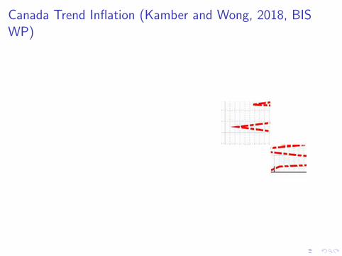
Canada Trend Inflation (Kamber and Wong, 2018, BISWP)

Decompose Trend Inflation and Inflation Gap
Source: Kamber and Wong (2018)

Share of Foreign Shocks (%) (Kamber and Wong, 2018,BIS WP)

Canadian Output Gap (Morley, Vehbi, and Wong)

Historical Decomposition of the Canadian Output Gap(Morley, Vehbi, and Wong)

Historical Decomposition of Canadian Trend Growth (YoY)(Morley, Vehbi, and Wong)

U.S. Output Gap (Benchmark Model)


Additional Slides
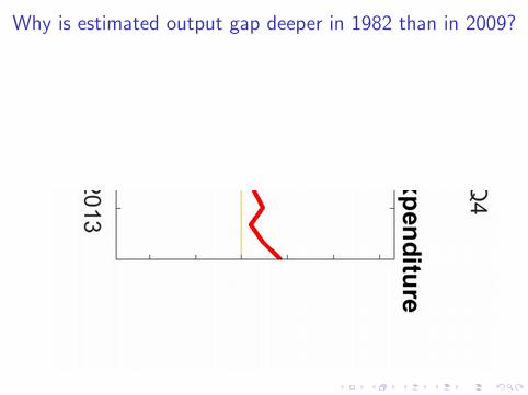
Why is estimated output gap deeper in 1982 than in 2009?
Recommended