International Journal of Mechanical Engineering and Applications 2016; 4(3): 115-122
http://www.sciencepublishinggroup.com/j/ijmea
doi: 10.11648/j.ijmea.20160403.13
ISSN: 2330-023X (Print); ISSN: 2330-0248 (Online)
Estimating On-Bottom Stability of Offshore Pipelines in Shallow Waters of the Gulf of Guinea
Ogbonda Douglas Chukwu1, Chinwuba Victor Ossia
1, C. O. Akhigbemidu
2
1Offshore Technology Institute, ETF Gas Engineering Building, University of Port Harcourt, Port Harcourt, Nigeria 2Project Masters Nigeria Limited, East-West Road, Port Harcourt, Nigeria
Email address:
[email protected] (C. V. Ossia)
To cite this article: Ogbonda Douglas Chukwu, Chinwuba Victor Ossia, C. O. Akhigbemidu. Estimating On-Bottom Stability of Offshore Pipelines in Shallow
Waters of the Gulf of Guinea. International Journal of Mechanical Engineering and Applications. Vol. 4, No. 3, 2016, pp. 115-122.
doi: 10.11648/j.ijmea.20160403.13
Received: May 14, 2016; Accepted: May 24, 2016; Published: June 13, 2016
Abstract: Pre-installation Stability analyses of pipelines are required to prevent lateral and upheaval buckling in service. In
this study, the hydrodynamic forces associated with an offshore pipeline is analyzed, thereby determining limiting steel wall-
thickness and submerged weight necessary to prevent collapse and propagation buckling, contain pressure and ensure on-
bottom stability. Relevant design equations, Codes and Procedures were integrated to create a comprehensive platform for
analyzing lift, drag and inertia forces acting on submerged pipelines. Hence, a user friendly template with multiple design
settings has been developed with MathCAD® for on-bottom stability analyses. The analysis tool is based on the absolute
lateral stability method in DNV RP F109. A case study of � 762 mm x 34 km pipeline to be installed Offshore Escravos, Gulf
of Guinea is simulated and analyzed using the design tool developed. Pipeline behavior under different environmental and
pipeline conditions such as water depth, wave height, steel and concrete thickness were investigated. The results showed that
concrete and steel wall thicknesses are the most critical parameters in the on-bottom stability of offshore pipelines. With a
determined optimal wall thickness of 20.6mm, concrete thicknesses of 78.796 mm, 61.386 mm, 53.043 mm and 42.58 mm
corresponding to 5 m, 10 m, 15 m and 20 m water depths, respectively were obtained. Also, the results showed that for pipes
OD > � 32.5 in (� 825.5 mm) alternative stability methods may be required as the necessary concrete thickness may exceed
allowable limits.
Keywords: Concrete Weight Coating, Concrete Coating Thickness, Pipeline Wall Thickness, On-Bottom Stability
1. Introduction
All submerged offshore pipelines and sections of onshore
pipelines in swamps, floodable areas, high water table areas,
river crossings etc., should be stable under the action of
hydrostatic and hydrodynamic forces [1]. The hydrodynamic
forces on the pipeline on the seabed are the combined action
of wave and current. It is important to correctly predict these
forces imposed on the pipeline since they have a direct
impact on the safety and economy of any pipeline project [2].
Ensuring the on bottom stability of an offshore pipeline on
the seabed is critical to that pipeline attaining and exceeding
its design life. On-bottom stability of pipelines is governed
by the fundamental balance between loads and resistances. In
offshore pipelines, these loads are hydrodynamic loads
induced by waves and currents. This load-resistance
relationship has formed the basis for various design codes
governing the stability of submarine pipelines such as the
API RP 1111 [3], DNV RP E305 [4], DNV RP F109 [5], and
DNV OS F101 [6].
Ensuring the stability of offshore pipelines involves
maintaining lateral stability (preventing the pipeline from
sliding sideways) and vertical stability (the pipeline being
stable on the seabed or buried). Predicting on-bottom
pipeline stability is complex requiring interdisciplinary
integration including; soil constitutive modeling, seabed
liquefaction, scour and sediment transport, structural
mechanics and prediction of ocean waves and hydrodynamic
loads. Considering this complexity, most pipelines are
designed using very simplified models [7].
The most common practice to achieve on bottom stability
116 Ogbonda Douglas Chukwu et al.: Estimating On-Bottom Stability of Offshore Pipelines in
Shallow Waters of the Gulf of Guinea
onshore is by application of sufficient concrete coating to
counteract buoyancy forces as it would not be economical to
increase steel wall thickness to a level that sufficiently weighs
down the pipeline. However in offshore pipelines, there are
practical limits to which concrete coating can be applied as
heavy pipelines imply high installation stresses on the lay
vessel and on the pipe itself. In the 1970s, the Coulomb theory
of soil friction was used to gauge soil resistance to the
displacement of submarine pipelines under hydrodynamic
loads such as waves and ocean currents [8]. This model adopts
a load-resistance relationship that ensures the pipe does not
displace horizontally i.e. hydrodynamic loading must not
exceed pipe and soil resistance. The DNV-RP-F109 [5] which
reflects state-of-the-art industry practice and latest research,
also utilizes the Load and Resistance Factors Design Format
(LRFD). This method places an upper (allowable) limit on
pipe displacement due to hydrodynamic loads, with target
safety levels given in the DNV-OS-F101 [6].
The DNV-OS-F101 [6] presents a force balance method
where a subsea pipeline has been considered stable if it has got
sufficient submerged weight so that the lateral soil resistance is
sufficiently high to restrain the pipeline from deflecting
sideways. The main stabilizing method has traditionally been
to apply sufficient amount of concrete weight coating (CWC).
The traditional design approach for subsea pipelines which is
expressed in the early design codes, such as “Rules for
Submarine Pipeline Systems" [9], was to not to allow for any
horizontal movement when a pipe is exposed to the
environmental conditions associated with an extreme return
period, i.e., a 100 year Return Period. Even if this method has
been widely replaced by the empirical or calibrated methods,
the force balance method is still in common use in cases where
a pipeline is exposed to pure current [10].
The design method presented in the DNV-RP-E305 [4]
relates to a pipeline resting on the seabed throughout its lifetime,
or prior to some other form of stabilization (e.g. trenching,
burial, self-burial). The stability of the pipeline is then directly
related to the submerged weight of the pipeline, the
environmental forces and the resistance developed by the seabed
soil. Consequently, the aim of stability design is to verify that the
submerged weight of the pipeline is sufficient to meet the
required stability criteria. Three different analysis methods were
used in this code. The Dynamic Stability Analysis method and
two simplified or calibrated methods that do not require full
dynamic FE analysis, namely, the Simplified and General
Stability Analysis methods. The Dynamic Stability Design
Method is based on a time-domain solution of the pipeline
stability and incorporates three-dimensional effects, surface
wave spectra and nonlinear soil resistance.
The Generalized method comprises a set of design response
curves which have been developed based on a large number of
dynamic FE simulations. The background for the methodology
is based on the assumption that the pipeline lateral
displacement is to a large extent a function of a relative small
number of non-dimensional parameters. The curves for use in
sandy soils are for net pipe movements of up to 40 pipe
diameters in DNV Zone 1 (more than 500 m away from a
platform) or 0 m in DNV Zone 2 (less than 500 m from a
platform). No displacement is allowed in clays. The curves are
based on pipe roughness and sea state spectrum (JONSWAP),
which helps determine the wave-induced velocity.
DNV recommends the Simplified Stability Design Method
based on a link between the traditional stability design
procedure and the generalized stability analysis. The results
from the two distinct methods are made consistent with each
other through the use of two calibration factors: one based on
the soil conditions, and one based on the Keulegan-Carpenter
number and ratio of wave to current velocity. The calibration
factors ensure that the results of the simplified analysis tie in
with the generalized analysis [11].
A calibration factor is multiplied by the submerged weight
determined from the traditional type design to arrive at the
new design submerged weight. The factor varies from 1.0 to
1.6. The calibration gives pipe weights that produce a
conservative envelope to the generalized procedure. For this
method, simplified design is characterized as;
� a hydrodynamic force (Morison type) formulation with
force coefficients 0.7, 0.9, and 3.29 for CD, CL, and CM
respectively and,
� a simple frictional soil resistance model with
coefficients of 0.7 for sand and 0.15 to 1.3 for clays.
The wave induced water particle velocity is taken as the
significant bottom velocity. This deviates from traditional
designs where the wave induced water velocity is normally
taken as that associated with the significant wave or
sometimes the maximum wave. This analysis is again based
on pipelines designed with an allowable lateral displacement
of up to 20 m in sandy soil and 0 m in clayey soil. As a result
of extensive research and developments performed in the
1980s in the area of pipeline stability, it was accepted that
some movement can be allowed during extreme sea states
provided that the lateral displacements were kept within
defined limits. This is reflected in the two calibrated
methods, the Simplified and the Generalized Methods, which
do not require Finite Element analyses. The limitations of
this code include:
� The code does not provide guidance on pipe-seabed
interaction forces for pipelines on carbonate soils;
� It does not allow for the effect of pipeline embedment
on soil resistance and hydrodynamic loading; and
� It does not consider the effects of seabed instability within
the response of the pipeline during storm loading [12].
This code has been replaced by the new DNV-RP-F109.
The DNV-RP-F109 was first published in 2007 and
updated in 2010, and it has superseded the old DNV-RP-
E305. This updated code does allow for some effects of
pipeline embedment. However, it does not consider
asymmetrical embedment levels, and also does not provide
quantitative guidance for carbonate soils. Three stability
analysis methods are included in this code. The Absolute
Lateral Static Stability method of the DNV-RP-F109 replaces
the force balance method of the DNV-OS-F101 [13] and the
simplified method of the DNV-RP-E305. It ensures that no
pipe motion will occur when the pipeline is exposed to
International Journal of Mechanical Engineering and Applications 2016; 4(3): 115-122 117
maximum load during sea state. This method appears to be
significantly more conservative than the more traditional
force balance method. In most situations, some minor pipe
movements (< 1m) can safely be allowed which will
significantly reduce the required pipeline submerged weight
[10]. As this method has evolved, the criteria for defining
pipeline stability have loosened and now extend to allowing
the pipeline to displace a significant predefined lateral
distance under a given load condition. This allowance leads
to the next two types of stability analysis methods [15].
The Generalized Lateral Stability Method of the DNV-RP-
F109 as opposed to the E305 which presented curves for
lateral displacements ranging from 0 to 40 times the external
pipe diameter. The new design code, F109 is based on a
lateral displacement limited to up to 10 pipe diameters during
a given sea state. But it follows similar design principles as
the respective method in E305.
The Dynamic Lateral Stability Analysis method is used to
predict the displacement of a pipeline during a design storm
event. Although the use of dynamic FE analyses to calculate
pipeline structural response is the most comprehensive
method available to assess pipeline stability, the method has
not been widely used by pipeline engineers for several
reasons. Firstly, in many locations around the world where
stability can readily be mitigated by applying a minimal
amount of Concrete Weight Coating (CWC), there has not
been a strong motivation for replacing the calibrated
(Simplified and Generalized) methods with a more advanced
FE-based method. Secondly, the design tools based on this
method are not easily available [10]. The limitations of the
DNV-RP-F109 are as follows:
� This code focuses on pipeline on-bottom stability with
relatively low embedment levels, and is not suited to the
assessment of highly embedded pipeline sections,
� This updated code allows for some effects of pipeline
embedment; however it does not consider asymmetrical
embedment levels, and also does not provide
quantitative guidance for carbonate soils,
� It does not consider the effects of the changes in seabed
bathymetry (seabed topography) during a storm event
on pipeline stability [12].
Three design procedures (Levels 1, 2 and 3) are presented in
AGA design guidelines and software [14]. The first procedure
(Level 1) is based on traditional stability analysis methods
(Morison type hydrodynamic forces and frictional soil
resistance). It is intended only as a reference to the type of
static analysis which has been done in the past. The most
detailed procedure uses finite element time domain simulation
software (Level 3). The software provides detailed information
regarding pipe movement and stresses during design events.
Pipeline safety is then assessed based on these results.
The Level 2 procedure assumes no net movement of the
pipe, and is based on a quasi-static calculation which
simulates the embedment process modeled in the Level 3
software. The process modeled is that of a pipe embedding
itself into the soil during small amplitude displacement
oscillations caused by wave loadings. The resulting lateral
soil resistance is calculated and compared to the expected
hydrodynamic forces to determine pipe stability. Levels 2
and 3 allow a much better representation of the sea state than
the “design wave" approach used in Level 1 [16]. The
limitations of AGA include:
� The AGA design code does not allow pipeline
displacement;
� The AGA hydrodynamic model is not based on field
measurement data, it's based solely on laboratory model
tests;
� The AGA design code does not assume a design sea
spectrum, but allows the user to specify the sea state
representation.
Some similarities exist between the AGA method and the
DNV-RP-F109’s method:
a) Both methods are based on very similar dynamic
simulation tools which use a FE pipeline model subject
to irregular waves plus steady current loadings.
b) Both methods include history dependent pipe-soil
interaction models, where soil resistance and pipe
embedment are based on recent pipe movement history.
c) Both are based on the assumption that the duration of
the design sea-state is 3 hours;
d) The hydrodynamic force formulations are quite
different between the two design tools. The resulting
forces produced by both models are very similar
though. This demonstrates the accuracy of the
hydrodynamic forces estimation.
The analysis methods in DNV-RP-F109 range from an
absolute stability where no movement of the pipeline is
allowed to a lateral displacement of up to 10 pipe diameters.
This range makes it a very versatile and flexible standard
which can be used for different types of purposes to which
the pipeline is intended. For the on-bottom stability analysis
procedures, it can be seen that, the DNV standard, which is
based on empirical design parameters, has a very detailed
approach compared to all other codes and standards. Besides,
DNV standard is regarded as a well-respected code to which
the majority of the other standards refer. Therefore, the
design procedures and sensitivity analyses in this work are
based on the state-of-the-art DNV-RP-F109 standard.
2. Methodology
2.1. Input Data
Data for this research was obtained from a pipeline
scheduled for installation at Offshore Escravos Oilfield in the
Niger Delta region. The data input for this study can be
categorized into pipeline properties, environmental data and
seabed properties.
The input data for pipelines properties of this study
include: Pipeline Wall Thickness t (mm) = 20.6 (calculated);
Corrosion Coating Thickness tcc (mm) = 5; Density of Steel
Material ρst (kg/m3) = 7850; Nominal Outer Diameter of
Steel Do (mm) = 30; Density of Corrosion Coating ρcc
(kg/m3) = 1300 (Single Layer FBE corrosion coating);
118 Ogbonda Douglas Chukwu et al.: Estimating On-Bottom Stability of Offshore Pipelines in
Shallow Waters of the Gulf of Guinea
Density of Concrete Coating ρc (kg/m3) = 3044; Density of
Seawater ρw (kg/m3) = 1025; Density of Field Joint Filler
coating ρfj (kg/m3) = 1026 (PUF - Polyurethane field joint)
when submerged); Joint Length Lpipe (m) = 12.19; Concrete
Cut-Back Length Lfj (mm) = 355.6. The density of pipeline
contents ρi (kg/m3) = 0 for Cases 1-4 (installation stage) and
855.691 for case-5 (pipeline operational stage – with oil and
gas); while the Concrete Coating Thickness tc (mm) specified
by client was 82.55, 76.2, 63.50 and 82.55 for Case-1, 2, 3, 4
and 5, respectively.
Relevant environmental data utilized in this study include:
Reduction due to wave spreading and directionality, R = 1;
Reference height above seabed zr (m) = 0.9144; Angle of
shallow wave with pipeline θ1(°) = 60; Concrete Water
Absorption ξ (%) = 4; Current Velocity at reference height Uref
(m/s) = 0.1542; Phase angle of the hydrodynamic force in the
wave cycle θ (°) = 0.360; Inertia Force Coefficient CM = 3.29;
Lift Force Coefficient CL = 0.9; Kinematic Viscosity v (m2/s) =
1.03ˣ10-6
; Current direction w.r.t. pipeline θcurr (°) = 90; Slope
of trench θslope (deg) = 30, 0, 0, 0 and 30 for case-1,2, 3, 4 and
case-5, respectively. Similarly, the pipeline burial depth H (m)
= 2, 0, 0, 0, and 2 for case-1, 2, 3, 4 and case-5, respectively.
Wave Spectral Peak Period Tp (s) = 16.6s for cases 1, 2, 3, 4,
and 17.9 for case-5. Water depth d (m) = 4, 10, 15, 20 and 5 for
case 1, 2, 3, 4 and case 5, respectively; whereas the significant
wave height Hs (m) = 2.262, 2.505, 2.804, 2.716 and 2.862 for
case 1, 2, 3, 4 and case 5, respectively.
Seabed grain size d50 and the undrained shear strength of
soil Su for Cases 1-5 were 0.0625mm and 224.338 kg/m2
(2.2in), respectively.
2.2. Design Assumptions for the Template Development
� No marine growth on the pipeline was considered.
� Current and waves acting perpendicular to the pipeline.
� Water Absorption as a percentage of concrete weight
was taken as 4%.
� The soil friction factor for the seabed is calculated
based on DNV-RP-E305 [4].
� The 10 year significant wave height and peak period
plus 1 year current are considered for the installation
condition. Pipeline is assumed to be empty for all
installation cases.
� The 100 year significant wave height and peak period
plus the 10 year current are considered for the operating
conditions (Case 5). Minimum internal product density
of 860kg.m-3
has been used.
2.3. Procedures / Algorithms
The following procedures leading to algorithm equations
(1) – (15) were adhered to in this study:
� The submerged weight of the pipeline in air and with
product taking buoyancy into consideration was
calculated using the algorithm;
�� = ��� + �� + �� ���
∙ �2 ∙ ��� ∙ ���� + � ∙ �� ∙ �� �����∙����� ���
∙ �� − (1)
� The corresponding significant water velocity was
interpolated from the Pierson Moskovitz curve [17] for
corresponding values of wave height Hs and Tn/Tp ratio
using the algorithm:
!�� = "#$�
∙ %&'()*+ ,-'.-+, 01, $�$2
3 (2)
� The zero up crossing period corresponding to the Tn/Tp
ratio was obtained using the algorithm:
-4 = -5 ∙ %&'()*+ ,-'.-+, -6-+, $�$2
3 (3)
In obtaining the calibration factor Fw as a function of
keulegan carpenter number K and current to wave ratio M,
the graphs from DNV-RP-E305 [4] for calibration factor was
transformed into a nested if statement below.
For M ≤ 0.2
78 = &9:; ≤ 5, 1.0, &9A; ≥ 25, 1.6, 0.03 ∙ E; − 5F + 1GH (4)
For 0.2 < M < 0.4
78 = &9:; ≤ 5, 1.0, &9A; ≥ 21.6, 1.5, 0.03 ∙ E; − 5F + 1GH (5)
For 0.4 ≤ M ≤ 0.6
78 = &9:; ≤ 5, 1.0, &9A; ≥ 18.3, 1.4, 0.03 ∙ E; − 5F + 1GH (6)
For 0.6 < M < 0.8
78 = &9:; ≤ 5, 1.0, &9A; ≥ 15.3, 1.3, 0.03 ∙ E; − 5F + 1GH (7)
Otherwise,
78 = &9:; ≤ 5, 1.0, &9A; ≥ 12, 1.2, 0.03 ∙ E; − 5F + 1GH (8)
� The Lift FL, Drag FD and Inertia forces FI acting on the
pipeline as a function of phase angle was calculated
using Morison’s equation. Considering lift and drag
trench reduction factors, the algorithm took the form:
7�EKF = L� ∙ 9MN ∙ �8 ∙ O ∙ P� ∙ E!� ∙ cos K + !�F� (9)
7TEKF = L� ∙ 9MU ∙ �8 ∙ O. PT ∙ |E!� ∙ cos K + !�F|E!� ∙ cos K + !�F (10)
7WEKF = X∙TYZ ∙ �8 ∙ P[ ∙ �� ∙ sin K (11)
For sections of the pipeline that are unburied, the lift and
drag trench reduction factors, frl and frx, do not apply.
� Citing Sec. 5.3.6 of DNV-RP-E305, the limiting value
of submerged weight, Wsmin, as a function of phase
angle, θ, was calculated using:
��^�_EKF = `�abEcFdaeEcF�df∙agEcFf h ∙ 78 (12)
The required minimum submerged weight to ensure lateral
stability, Wsubreq, is given as the maximum limiting value of
submerged weight over a wave cycle. This value is obtained
through using MathCad command by Mathsoft [18]:
��4iMjk = lmn���^�_EKF� (13)
International Journal of Mechanical Engineering and Applications 2016; 4(3): 115-122 119
� To find the required area of concrete coating, Ac_req,
iteration was carried out in MathCad to find the area of
concrete coating that satisfies the condition:
��4iMjk = ��o · ��o � ��� · ���
� ����p�_o
:���p�_o � 2 · ���� · ��H � �� � ����p�_o
�2 · ��� · ����
�� · �� · �� �����·����� ���
· �� � �8 q�� � X·TrrY
Z s (14)
� To find the required concrete coating thickness, tc_req,
iteration was carried out in MathCad to find the
concrete coating thickness that satisfied the condition:
��_Mjk � u · �O�� · (�_Mjk � (�_Mjk� � (15)
3. Results and Discussions
The primary objective of pipeline design it to optimize the
relationship between pipe diameter, pipe material, pipe wall
thickness, appurtenances, economics, constructability and
operability of the pipeline. Raw input data (from section 2.1)
were inputted into the Mathcad template created in sections
2.2 and 2.3 above.
3.1. Hydrodynamic Forces
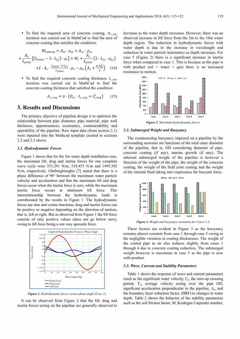
Figure 1 shows that for the 5m water depth installation case,
the maximum lift, drag and inertia forces for one complete
wave cycle were 333.291 N/m, 518.453 N/m and 1495.392
N/m, respectively. Ghebreghiorghis [7] stated that there is a
phase difference of 90° between the maximum water particle
velocity and acceleration and that the maximum lift and drag
forces occur when the inertia force is zero, while the maximum
inertia force occurs at minimum lift force. This
interrelationship between the hydrodynamic loads is
corroborated by the results in Figure 1. The hydrodynamic
forces are sine and cosine functions, drag and inertia forces can
be positive or negative depending on the direction of motion,
that is, left or right. But as observed from Figure 1 the lift force
consists of only positive values (does not go below zero),
owing to lift force being a one way upwards force.
Figure 1. Hydrodynamic forces versus phase angle (Case 1).
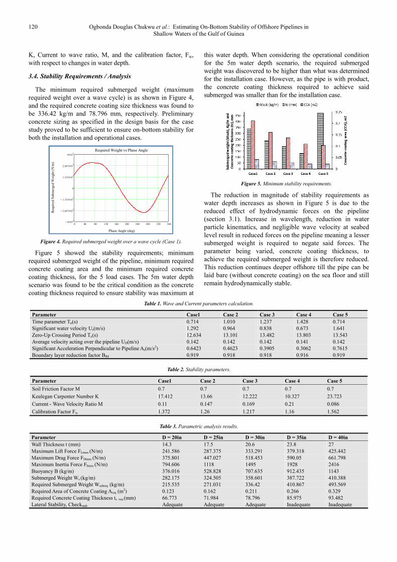
It can be observed from Figure 2 that the lift, drag and
inertia forces acting on the pipeline are generally observed to
decrease as the water depth increases. However, there was an
observed increase in lift force from the 5m to the 10m water
depth region. The reduction in hydrodynamic forces with
water depth is due to the increase in wavelength and
reduction in water particle kinematics as depth increases. For
case 5 (Figure 2) there is a significant increase in inertia
force when compared to case 1. This is because as the pipe is
with product (oil + water + gas) there is an increased
resistance to motion.
Figure 2. Maximum hydrodynamic forces.
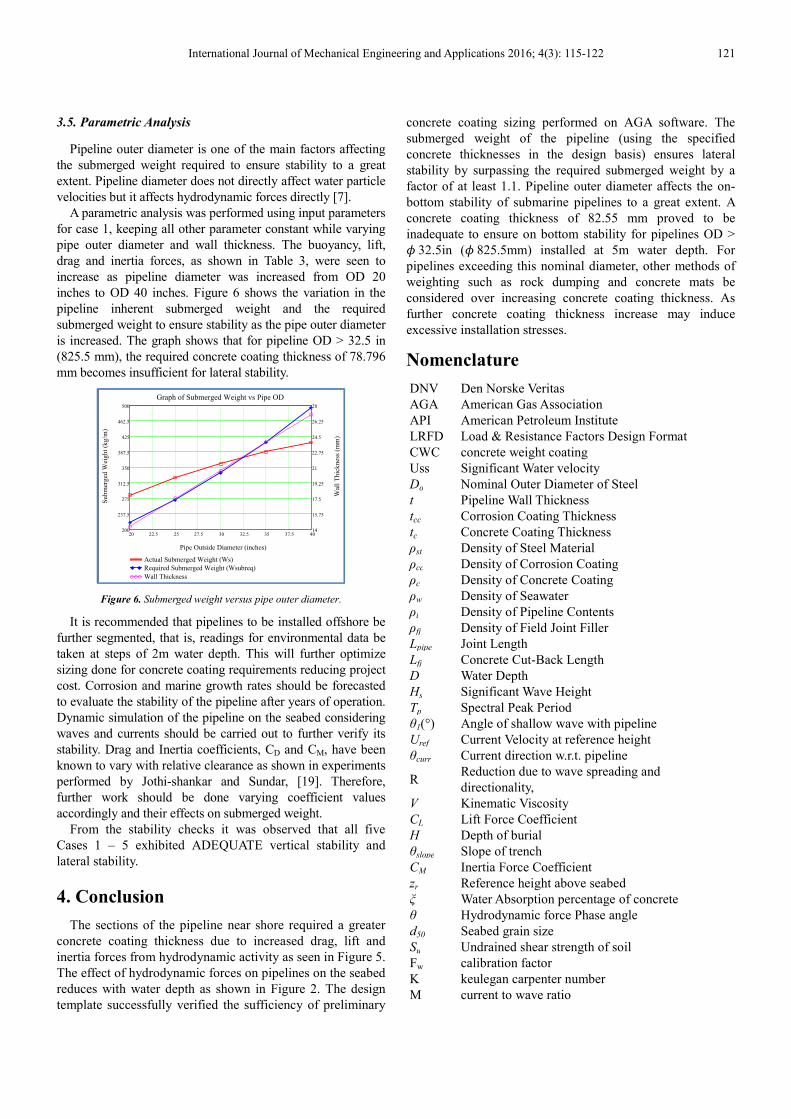
3.2. Submerged Weight and Buoyancy
The counteracting buoyancy imposed on a pipeline by the
surrounding seawater are functions of the total outer diameter
of the pipeline, that is, OD considering diameter of pipe,
concrete coating (if any), marine growth (if any). The
inherent submerged weight of the pipeline is however a
function of the weight of the pipe, the weight of the concrete
coating, the weight of the field joint coating and the weight
of the internal fluid taking into cognizance the buoyant force.
Figure 3. Weight and buoyancy variations for Cases 1-5.
These factors are evident in Figure 3 as the buoyancy
remains almost constant from case 1 through case 5 owing to
the negligible variation in coating thicknesses. The weight of
the coated pipe in air also reduces slightly from cases 1
through 4 due to concrete coating reduction. The submerged
weight however is maximum in case 5 as the pipe is now
with product.
3.3. Wave, Current and Stability Parameters
Table 1 shows the response of wave and current parameters
(such as the significant water velocity, Us, the zero-up crossing
period, Tu, average velocity acting over the pipe OD,
significant acceleration perpendicular to the pipeline, As, and
the boundary layer reduction factor, (BRF) to changes in water
depth. Table 2 shows the behavior of the stability parameters
such as the soil friction factor, M, Keulegan Carpenter number,
0 40 80 120 160 200 240 280 320 3601.6− 10
3×
1.28− 103×
960−
640−
320−
0
320
640
960
1.28 103×
1.6 103×
Inertia Force
Drag Force
Lift Force
Graph of Hydrodynamic Forces vs Phase Angle
Phase Angle (deg)
Fo
rces
(N
/m)
120 Ogbonda Douglas Chukwu et al.: Estimating On-Bottom Stability of Offshore Pipelines in
Shallow Waters of the Gulf of Guinea
K, Current to wave ratio, M, and the calibration factor, Fw,
with respect to changes in water depth.
3.4. Stability Requirements / Analysis
The minimum required submerged weight (maximum
required weight over a wave cycle) is as shown in Figure 4,
and the required concrete coating size thickness was found to
be 336.42 kg/m and 78.796 mm, respectively. Preliminary
concrete sizing as specified in the design basis for the case
study proved to be sufficient to ensure on-bottom stability for
both the installation and operational cases.
Figure 4. Required submerged weight over a wave cycle (Case 1).
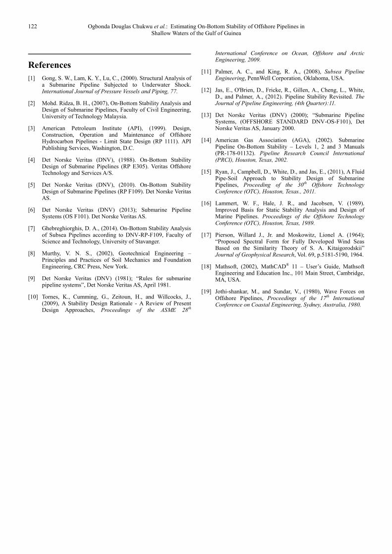
Figure 5 showed the stability requirements; minimum
required submerged weight of the pipeline, minimum required
concrete coating area and the minimum required concrete
coating thickness, for the 5 load cases. The 5m water depth
scenario was found to be the critical condition as the concrete
coating thickness required to ensure stability was maximum at
this water depth. When considering the operational condition
for the 5m water depth scenario, the required submerged
weight was discovered to be higher than what was determined
for the installation case. However, as the pipe is with product,
the concrete coating thickness required to achieve said
submerged was smaller than for the installation case.
Figure 5. Minimum stability requirements.
The reduction in magnitude of stability requirements as
water depth increases as shown in Figure 5 is due to the
reduced effect of hydrodynamic forces on the pipeline
(section 3.1). Increase in wavelength, reduction in water
particle kinematics, and negligible wave velocity at seabed
level result in reduced forces on the pipeline meaning a lesser
submerged weight is required to negate said forces. The
parameter being varied, concrete coating thickness, to
achieve the required submerged weight is therefore reduced.
This reduction continues deeper offshore till the pipe can be
laid bare (without concrete coating) on the sea floor and still
remain hydrodynamically stable.
Table 1. Wave and Current parameters calculation.
Parameter Case1 Case 2 Case 3 Case 4 Case 5
Time parameter Tn(s) 0.714 1.010 1.237 1.428 0.714
Significant water velocity Us(m/s) 1.292 0.964 0.838 0.673 1.641
Zero-Up Crossing Period Tu(s) 12.634 13.101 13.482 13.803 13.543
Average velocity acting over the pipeline UD(m/s) 0.142 0.142 0.142 0.141 0.142
Significant Acceleration Perpendicular to Pipeline As(m/s2) 0.6423 0.4623 0.3905 0.3062 0.7615
Boundary layer reduction factor BRF 0.919 0.918 0.918 0.916 0.919
Table 2. Stability parameters.
Parameter Case1 Case 2 Case 3 Case 4 Case 5
Soil Friction Factor M 0.7 0.7 0.7 0.7 0.7
Keulegan Carpenter Number K 17.412 13.66 12.222 10.327 23.723
Current - Wave Velocity Ratio M 0.11 0.147 0.169 0.21 0.086
Calibration Factor Fw 1.372 1.26 1.217 1.16 1.562
Table 3. Parametric analysis results.
Parameter D = 20in D = 25in D = 30in D = 35in D = 40in
Wall Thickness t (mm) 14.3 17.5 20.6 23.8 27
Maximum Lift Force FLmax (N/m) 241.586 287.375 333.291 379.318 425.442
Maximum Drag Force FDmax (N/m) 375.801 447.027 518.453 590.05 661.798
Maximum Inertia Force FImax (N/m) 794.606 1118 1495 1928 2416
Buoyancy B (kg/m) 376.016 528.828 707.635 912.435 1143
Submerged Weight Ws (kg/m) 282.175 324.505 358.601 387.722 410.388
Required Submerged Weight Wsubreq (kg/m) 215.535 271.031 336.42 410.867 493.569
Required Area of Concrete Coating Areq (m2) 0.123 0.162 0.211 0.266 0.329
Required Concrete Coating Thickness tc_req (mm) 66.773 71.984 78.796 85.975 93.482
Lateral Stability, Checkstab Adequate Adequate Adequate Inadequate Inadequate
0 40 80 120 160 200 240 280 320 3604− 10
3×
2.667− 103×
1.333− 103×
0
1.333 103×
2.667 103×
4 103×
Required Weight vs Phase Angle
Phase Angle (deg)
Req
uir
ed S
ubm
erged
Wei
ght
(N/m
)
International Journal of Mechanical Engineering and Applications 2016; 4(3): 115-122 121
3.5. Parametric Analysis
Pipeline outer diameter is one of the main factors affecting
the submerged weight required to ensure stability to a great
extent. Pipeline diameter does not directly affect water particle
velocities but it affects hydrodynamic forces directly [7].
A parametric analysis was performed using input parameters
for case 1, keeping all other parameter constant while varying
pipe outer diameter and wall thickness. The buoyancy, lift,
drag and inertia forces, as shown in Table 3, were seen to
increase as pipeline diameter was increased from OD 20
inches to OD 40 inches. Figure 6 shows the variation in the
pipeline inherent submerged weight and the required
submerged weight to ensure stability as the pipe outer diameter
is increased. The graph shows that for pipeline OD > 32.5 in
(825.5 mm), the required concrete coating thickness of 78.796
mm becomes insufficient for lateral stability.
Figure 6. Submerged weight versus pipe outer diameter.
It is recommended that pipelines to be installed offshore be
further segmented, that is, readings for environmental data be
taken at steps of 2m water depth. This will further optimize
sizing done for concrete coating requirements reducing project
cost. Corrosion and marine growth rates should be forecasted
to evaluate the stability of the pipeline after years of operation.
Dynamic simulation of the pipeline on the seabed considering
waves and currents should be carried out to further verify its
stability. Drag and Inertia coefficients, CD and CM, have been
known to vary with relative clearance as shown in experiments
performed by Jothi-shankar and Sundar, [19]. Therefore,
further work should be done varying coefficient values
accordingly and their effects on submerged weight.
From the stability checks it was observed that all five
Cases 1 – 5 exhibited ADEQUATE vertical stability and
lateral stability.
4. Conclusion
The sections of the pipeline near shore required a greater
concrete coating thickness due to increased drag, lift and
inertia forces from hydrodynamic activity as seen in Figure 5.
The effect of hydrodynamic forces on pipelines on the seabed
reduces with water depth as shown in Figure 2. The design
template successfully verified the sufficiency of preliminary
concrete coating sizing performed on AGA software. The
submerged weight of the pipeline (using the specified
concrete thicknesses in the design basis) ensures lateral
stability by surpassing the required submerged weight by a
factor of at least 1.1. Pipeline outer diameter affects the on-
bottom stability of submarine pipelines to a great extent. A
concrete coating thickness of 82.55 mm proved to be
inadequate to ensure on bottom stability for pipelines OD >
� 32.5in (� 825.5mm) installed at 5m water depth. For
pipelines exceeding this nominal diameter, other methods of
weighting such as rock dumping and concrete mats be
considered over increasing concrete coating thickness. As
further concrete coating thickness increase may induce
excessive installation stresses.
Nomenclature
DNV Den Norske Veritas
AGA American Gas Association
API American Petroleum Institute
LRFD Load & Resistance Factors Design Format
CWC concrete weight coating
Uss Significant Water velocity
Do Nominal Outer Diameter of Steel
t Pipeline Wall Thickness
tcc Corrosion Coating Thickness
tc Concrete Coating Thickness
ρst Density of Steel Material
ρcc Density of Corrosion Coating
ρc Density of Concrete Coating
ρw Density of Seawater
ρi Density of Pipeline Contents
ρfj Density of Field Joint Filler
Lpipe Joint Length
Lfj Concrete Cut-Back Length
D Water Depth
Hs Significant Wave Height
Tp Spectral Peak Period
θ1(°) Angle of shallow wave with pipeline
Uref Current Velocity at reference height
θcurr Current direction w.r.t. pipeline
R Reduction due to wave spreading and
directionality,
V Kinematic Viscosity
CL Lift Force Coefficient
H Depth of burial
θslope Slope of trench
CM Inertia Force Coefficient
zr Reference height above seabed
ξ Water Absorption percentage of concrete
θ Hydrodynamic force Phase angle
d50 Seabed grain size
Su Undrained shear strength of soil
Fw calibration factor
K keulegan carpenter number
M current to wave ratio
20 22.5 25 27.5 30 32.5 35 37.5 40200
237.5
275
312.5
350
387.5
425
462.5
500
14
15.75
17.5
19.25
21
22.75
24.5
26.25
28
Actual Submerged Weight (Ws)
Required Submerged Weight (Wsubreq)
Wall Thickness
Graph of Submerged Weight vs Pipe OD
Pipe Outside Diameter (inches)
Su
bm
erg
ed W
eig
ht
(kg
/m)
Wal
l T
hic
kn
ess
(mm
)
122 Ogbonda Douglas Chukwu et al.: Estimating On-Bottom Stability of Offshore Pipelines in
Shallow Waters of the Gulf of Guinea
References
[1] Gong, S. W., Lam, K. Y., Lu, C., (2000). Structural Analysis of a Submarine Pipeline Subjected to Underwater Shock. International Journal of Pressure Vessels and Piping, 77.
[2] Mohd. Ridza, B. H., (2007), On-Bottom Stability Analysis and Design of Submarine Pipelines, Faculty of Civil Engineering, University of Technology Malaysia.
[3] American Petroleum Institute (API), (1999). Design, Construction, Operation and Maintenance of Offshore Hydrocarbon Pipelines - Limit State Design (RP 1111). API Publishing Services, Washington, D.C.
[4] Det Norske Veritas (DNV), (1988). On-Bottom Stability Design of Submarine Pipelines (RP E305). Veritas Offshore Technology and Services A/S.
[5] Det Norske Veritas (DNV), (2010). On-Bottom Stability Design of Submarine Pipelines (RP F109). Det Norske Veritas AS.
[6] Det Norske Veritas (DNV) (2013); Submarine Pipeline Systems (OS F101). Det Norske Veritas AS.
[7] Ghebreghiorghis, D. A., (2014). On-Bottom Stability Analysis of Subsea Pipelines according to DNV-RP-F109, Faculty of Science and Technology, University of Stavanger.
[8] Murthy, V. N. S., (2002), Geotechnical Engineering – Principles and Practices of Soil Mechanics and Foundation Engineering, CRC Press, New York.
[9] Det Norske Veritas (DNV) (1981); “Rules for submarine pipeline systems”, Det Norske Veritas AS, April 1981.
[10] Tornes, K., Cumming, G., Zeitoun, H., and Willcocks, J., (2009), A Stability Design Rationale - A Review of Present Design Approaches, Proceedings of the ASME 28th
International Conference on Ocean, Offshore and Arctic Engineering, 2009.
[11] Palmer, A. C., and King, R. A., (2008), Subsea Pipeline Engineering, PennWell Corporation, Oklahoma, USA.
[12] Jas, E., O'Brien, D., Fricke, R., Gillen, A., Cheng, L., White, D., and Palmer, A., (2012). Pipeline Stability Revisited. The Journal of Pipeline Engineering, (4th Quarter):11.
[13] Det Norske Veritas (DNV) (2000); “Submarine Pipeline Systems, (OFFSHORE STANDARD DNV-OS-F101), Det Norske Veritas AS, January 2000.
[14] American Gas Association (AGA), (2002). Submarine Pipeline On-Bottom Stability – Levels 1, 2 and 3 Manuals (PR-178-01132). Pipeline Research Council International (PRCI), Houston, Texas, 2002.
[15] Ryan, J., Campbell, D., White, D., and Jas, E., (2011), A Fluid Pipe-Soil Approach to Stability Design of Submarine Pipelines, Proceeding of the 30th Offshore Technology Conference (OTC), Houston, Texas., 2011.
[16] Lammert, W. F., Hale, J. R., and Jacobsen, V. (1989). Improved Basis for Static Stability Analysis and Design of Marine Pipelines. Proceedings of the Offshore Technology Conference (OTC), Houston, Texas, 1989.
[17] Pierson, Willard J., Jr. and Moskowitz, Lionel A. (1964); “Proposed Spectral Form for Fully Developed Wind Seas Based on the Similarity Theory of S. A. Kitaigorodskii” Journal of Geophysical Research, Vol. 69, p.5181-5190, 1964.
[18] Mathsoft, (2002), MathCAD® 11 – User’s Guide, Mathsoft Engineering and Education Inc., 101 Main Street, Cambridge, MA, USA.
[19] Jothi-shankar, M., and Sundar, V., (1980), Wave Forces on Offshore Pipelines, Proceedings of the 17th International Conference on Coastal Engineering, Sydney, Australia, 1980.
Recommended