Evolutionary ComputationEvolutionary Computation(( 진 화 연 산진 화 연 산 ))
장 병 탁서울대 컴퓨터공학부
E-mail: [email protected]://scai.snu.ac.kr./~btzhang/
Byoung-Tak ZhangSchool of Computer Science and Engineering
Seoul National University
This material is also available online at http://scai.snu.ac.kr/

2
OutlineOutline
1. Basic Concepts
2. Theoretical Backgrounds
3. Applications
4. Current Issues
5. References and URLs

3
1. Basic Concepts1. Basic Concepts

4
Charles Darwin (1859)
“Owing to this struggle for life, any variation, however slight and from whatever cause proceeding, if it be in any degree profitable to an individual of any species, in its infinitely complex relations to other organic beings and to external nature, will tend to the preservation of that individual, and will generally be inherited by its offspring.”

5
Evolutionary AlgorithmsEvolutionary Algorithms
A Computational Model Inspired by Natural Evolution and Genetics
Proved Useful for Search, Machine Learning and Optimization
Population-Based Search (vs. Point-Based Search) Probabilistic Search (vs. Deterministic Search) Collective Learning (vs. Individual Learning) Balance of Exploration (Global Search) and Exploitation
(Local Search)

6
Biological TerminologyBiological Terminology
Gene Functional entity that codes for a specific feature e.g. eye color Set of possible alleles
Allele Value of a gene e.g. blue, green, brown Codes for a specific variation of the gene/feature
Locus Position of a gene on the chromosome
Genome Set of all genes that define a species The genome of a specific individual is called genotype The genome of a living organism is composed of several Chromosomes
Population Set of competing genomes/individuals

7
Analogy to Analogy to Evolutionary BiologyEvolutionary Biology Individual (Chromosome) = Possible Solution Population = A Collection of Possible Solutions Fitness = Goodness of Solutions Selection (Reproduction) = Survival of the Fittest Crossover = Recombination of Partial Solutions Mutation = Alteration of an Existing Solution

8
The Evolution LoopThe Evolution Loop
select mating partners
recombine
mutate
evaluate
select
(terminate)
evaluate
initialize population

9
Basic Evolutionary AlgorithmBasic Evolutionary Algorithm
Generation of initial solutions (A priori knowledge, results of earlier run, random)
Evaluation
Selection
SolutionSufficiently
good?
END
Generation of variants by mutation
and crossover
YES
NO
10
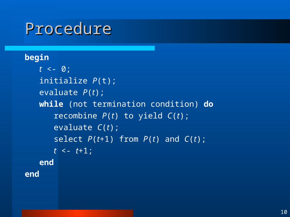
ProcedureProcedure
begin
t <- 0;
initialize P(t);
evaluate P(t);
while (not termination condition) do
recombine P(t) to yield C(t);
evaluate C(t);
select P(t+1) from P(t) and C(t);
t <- t+1;
end
end
11
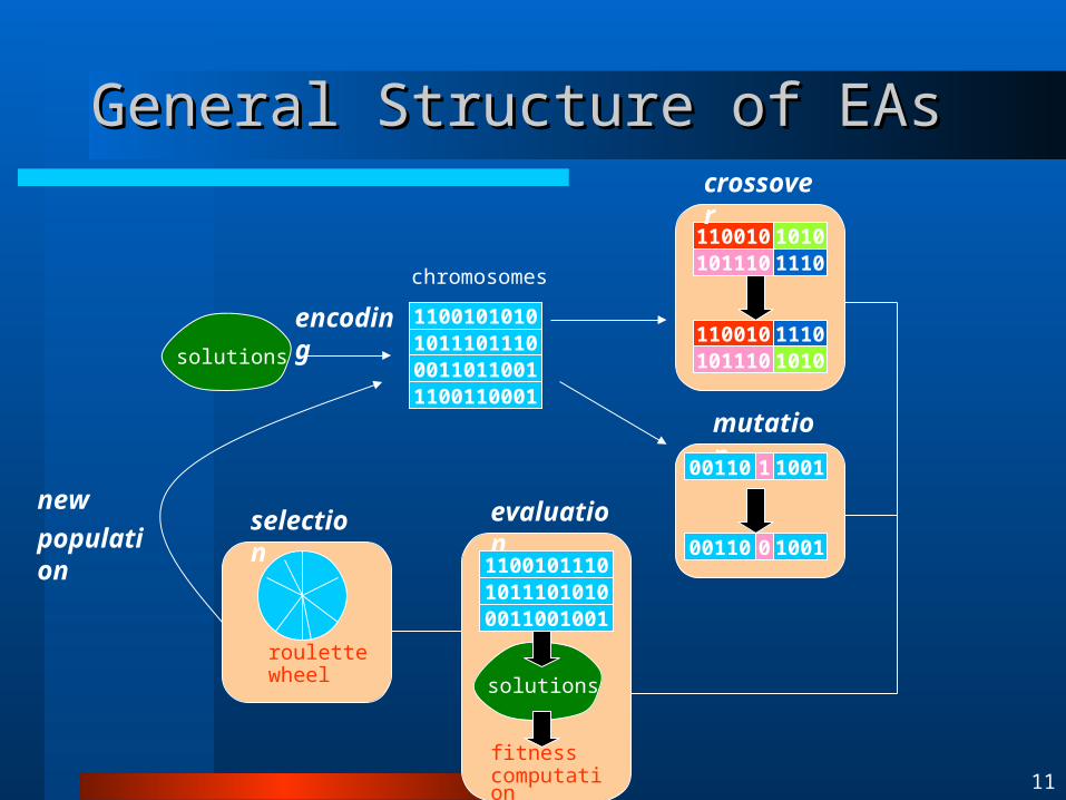
General Structure of EAsGeneral Structure of EAs
solutions
1100101010101110111000110110011100110001
1100101110
10111011101100101010
crossover
mutation
00110
1011101010
10011
00110 10010
evaluation
110010111010111010100011001001
solutions
fitnesscomputation
roulettewheel
selectionnew
population
encoding
chromosomes
12
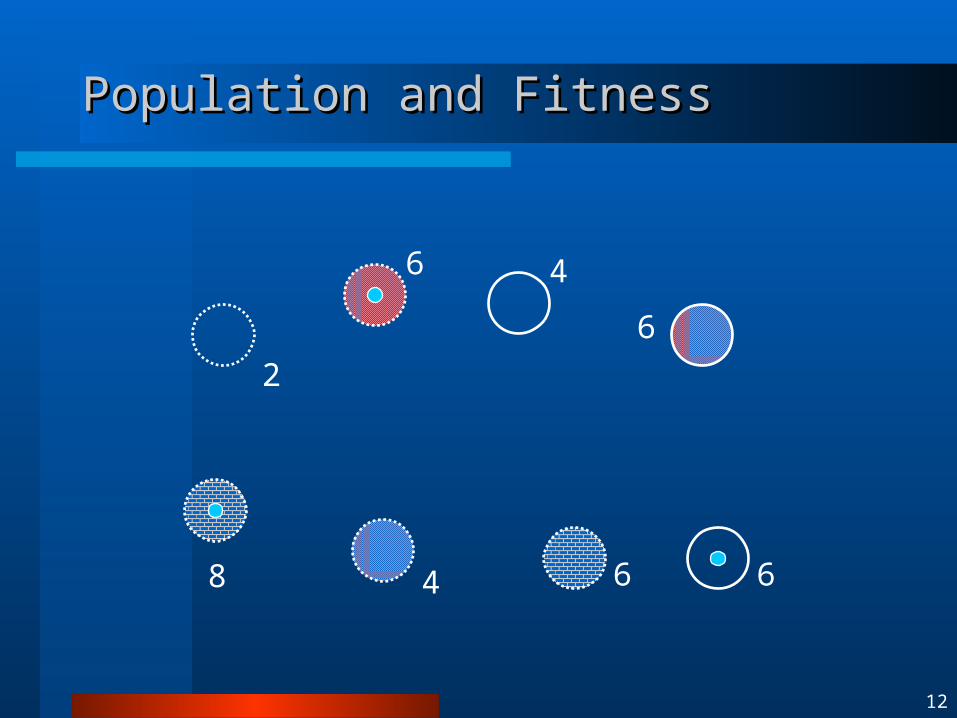
Population and FitnessPopulation and Fitness
2
4
6 4
668
6

13
Selection, Crossover, and MutationSelection, Crossover, and Mutation
Reproduction
Distinction Mutation
Crossover2
4
6 4
8
66
10
8
8
6

14
Simulated EvolutionSimulated Evolution
Population (chromosomes)
Geneticoperators
Selection(mating pool)
Evaluation (fitness)
Decodedstrings
Newgeneration
Offspring
Mating
Manipulation
Reproduction
Parents

15
Selection StrategiesSelection Strategies
Proportionate Selection Reproduce offspring in proportion to fitness fi.
Ranking Selection Select individuals according to rank(fi).
Tournament Selection Choose q individuals at random, the best of which survives.
Other Ways
1j
tj
tit
isaf
afap
i
iap t
is
,0
1,1
qtis iiap
1
1

16
Roulette Wheel SelectionRoulette Wheel Selection
10001
11010
01011
00101
10001
11010
01011
00101
1000
1
1101
0
0101
100
101
10001
11010 0101100101
1000111010
0101100101
intermediate parent population:
01011 11010 10001 10001
Probability of reproduction pi = fi / Sk fk
Selection is a stochastic process
17
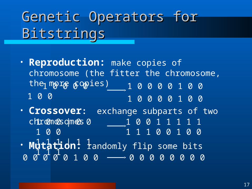
Genetic Operators for BitstringsGenetic Operators for Bitstrings
• Reproduction: make copies of chromosome (the fitter the chromosome, the more copies)
1 0 0 0 0 1 0 0
• Crossover: exchange subparts of two chromosomes
• Mutation: randomly flip some bits
1 0 0 | 0 0 1 0 0 1 1 1 | 1 1 1 1 1 0 0 0 0 0 1 0 0
1 0 0 0 0 1 0 0
1 0 0 0 0 1 0 0
1 0 0 1 1 1 1 1 1 1 1 0 0 1 0 0
0 0 0 0 0 0 0 0

18
MutationMutation
For a binary string, just randomly “flip” a bit For a more complex structure, randomly select a
site, delete the structure associated with this site, and randomly create a new sub-structure
Some EAs just use mutation (no crossover) Normally, however, mutation is used to search in
the “local search space”, by allowing small changes in the genotype (and therefore hopefully in the phenotype)

19
Recombination (Crossover)Recombination (Crossover)
Crossover is used to swap (fit) parts of individuals, in a similar way to sexual reproduction
Parents are selected based on fitness Crossover sites selected (randomly, although other
mechanisms exist), with some prob. Parts of the parents are exchanged to produce
children

20
CrossoverCrossover
One-point crossover
parent Aparent B
1 1 0 1 0
1 0 0 0 1
offspring Aoffspring B
1 1 0 1 1
1 0 0 0 0
Two-point crossover
parent Aparent B
1 1 0 1 0
1 0 0 0 1
offspring Aoffspring B
1 1 0 0
1 0 0 1
0
1

21
2. Theoretical Backgrounds2. Theoretical Backgrounds

22
Major Evolutionary AlgorithmsMajor Evolutionary Algorithms
Genetic Programming
Evolution Strategies
Genetic Algorithms Evolutionary
ProgrammingClassifier Systems
• Genetic representation of candidate solutions• Genetic operators• Selection scheme• Problem domain
Hybrids: BGA

23
Variants of Evolutionary AlgorithmsVariants of Evolutionary Algorithms
Genetic Algorithm (Holland et al., 1960’s) Bitstrings, mainly crossover, proportionate selection
Evolution Strategy (Rechenberg et al., 1960’s) Real values, mainly mutation, truncation selection
Evolutionary Programming (Fogel et al., 1960’s) FSMs, mutation only, tournament selection
Genetic Programming (Koza, 1990) Trees, mainly crossover, proportionate selection
Hybrids: BGA (Muehlenbein et al., 1993) BGP (Zhang et al., 1995) and others.

24
Evolution Strategy (ES)Evolution Strategy (ES)
Problem of real-valued optimizationFind extremum (minimum) of function F(X): Rn ->R
Operate directly on real-valued vector X Generate new solutions through Gaussian
mutation of all components Selection mechanism for determining new parents

25
ES: RepresentationES: Representation
One individual:
The three parts of an individual:
Ixxa nnn
,,,,,,,, 111
x
: Object variables
: Standard deviations
: Rotation angles
Fitness
Variances
Covariances
)(xf
x

26
, where rx, r , r {-, d, D, i, I, g, G}, e.g. rdII rrr xr
GiSiTiiS
giSiTiS
IiSiTiS
iiSiTiS
DiTiS
diTiS
iS
i
rxxx
rxxx
rxxx
rxxx
rxx
rxx
rx
x
i
i
i
teintermedia dgeneralize panmictic)(
teintermedia dgeneralize)(
teintermedia panmictic2/)(
teintermedia2/)(
discrete panmicticor
discreteor
ionrecombinat no
,,,
,,,
,,,
,,,
,,
,,
,
ES: Operator - RecombinationES: Operator - Recombination

27
m{,’,} : I I is an asexual operator. n = n, n = n(n-1)/2
1 < n < n, n = 0
n = 1, n = 0
)),(,0(
)1,0(
))1,0()1,0(exp(
CNxx
N
NN
jjj
iii
0873.0
2
2
1
1
n
n
)1,0(
))1,0()1,0(exp(
iiii
iii
Nxx
NN
)1,0(
))1,0(exp( 0
iii Nxx
N
n/10
ES: Operator - MutationES: Operator - Mutation

28
ES: Illustration of Mutation ES: Illustration of Mutation HyperellipsoidsHyperellipsoids
Line of equal probability density to place an offspring

29
ES: Evolution Strategy vs. ES: Evolution Strategy vs. Genetic AlgorithmGenetic Algorithm
Create random initial population
Evaluate population
Select individuals for variation
Vary
Insert intopopulation
Create random initial population
Evaluate population
Vary
Selection
Insert intopopulation

30
Evolutionary Programming (EP) Evolutionary Programming (EP)
Original form (L. J. Fogel) Uniform random mutations Discrete alphabets selection
Extended Evolutionary Programming (D. B. Fogel) Continuous parameter optimization Similarities with ES
• Normally distributed mutation
• Self-adaptation of mutation parameters
)(

31
EP: RepresentationEP: Representation
Constraints for domain and variances Initialization only-operators does not survey
• Search space is principally unconstrained.
Individual
EP) (metaor EP) (std and
,),(n
ssn
x
sx
RAARA
AAIxa
32
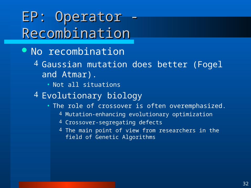
EP: Operator - RecombinationEP: Operator - Recombination
No recombination Gaussian mutation does better (Fogel and Atmar).
• Not all situations
Evolutionary biology• The role of crossover is often overemphasized.
Mutation-enhancing evolutionary optimization Crossover-segregating defects The main point of view from researchers in the field of Genetic
Algorithms

33
EP: Operator - MutationEP: Operator - Mutation
General form (std. EP)
Exogenous parameters must be tuned for a particular task
Usually Problem
• If global minimum’s fitness value is not zero, exact approachment is not possible
• If fitness values are very large, the search is almost random walk
• If user does not know about approximate position of global minimum, parameter tuning is not possible
)1,0()( iiiii Nxxx
ii ,
)1,0()( iii Nxxx

34
EP: Differences from ESEP: Differences from ES
Procedures for self-adaptation Deterministic vs. Probabilistic selection -ES vs. -EP Level of abstraction: Individual vs. Species
),( )(

35
Genetic ProgrammingGenetic Programming
Applies principles of natural selection to computer search and optimization problems - has advantages over other procedures for “badly behaved” solution spaces [Koza, 1992]
Genetic programming uses variable-size tree-representations rather than fixed-length strings of binary values.
Program tree
= S-expression
= LISP parse tree Tree = Functions (Nonterminals) + Terminals

36
GP: RepresentationGP: Representation
S-expression: (+ 1 2 (IF (> TIME 10) 3 4))Terminals = {1, 2, 3, 4, 10, TIME}Functions = {+, >, IF}
+
2
4> 3
1 IF
TIME 10
37
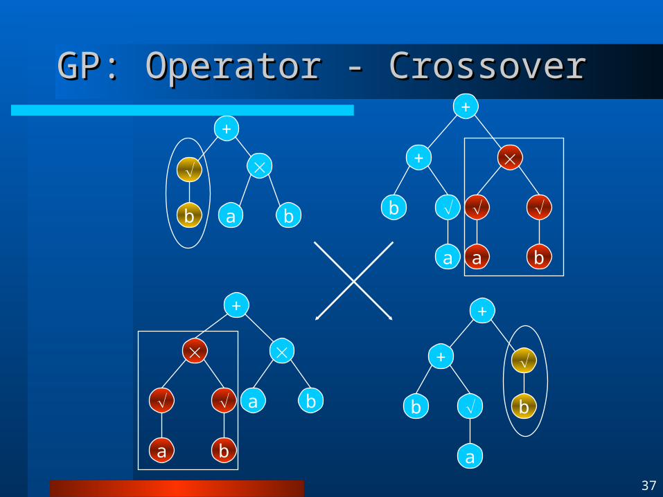
GP: Operator - CrossoverGP: Operator - Crossover
+
b
a b
+
b
+
a a b
+
a b
a b
+
b
+
a
b

38
GP: Operator - MutationGP: Operator - Mutation
a b
+
b
/
a
+
b
+
b
/
a
-
b a

39
Breeder GP (BGP) Breeder GP (BGP) [Zhang and Muehlenbein, 1993, 1995][Zhang and Muehlenbein, 1993, 1995]
ES (real-vector) GA (bitstring)
Breeder GA (BGA)(real-vector + bitstring)
GP (tree)
Breeder GP (BGP)(tree + real-vector + bitstring)
Muehlenbein et al. (1993)
Zhang et al. (1993)

40
GAs: Theory of Simple GAGAs: Theory of Simple GA
Assumptions Bitstrings of fixed size Proportionate selection
Definitions Schema H: A set of substrings (e.g., H = 1**0) Order o: number of fixed positions (FP) (e.g., o(H) = 2) Defining length d: distance between leftmost FP and
rightmost FP (e.g., d(H) = 3)

41
GAs: Schema Theorem (Holland GAs: Schema Theorem (Holland et al. 1975)et al. 1975)
)(11
)(1
)(
),(),()1,( Ho
mc pn
Hdp
tf
tHftHmtHm
),( tHm
cp mp ,
Number of members of H
Probability of crossover and mutation, respectively
Interpretation: Fit, short, low-order schemata (or building blocks) exponentially grow.

42
Convergence velocity of (+, )-ES
ES-),( afor and ES-)( afor 0 where
)1(11
minmin
1
1),(
min
kk
kdpppv
k vkk
vkkkkkk
vjjj
8erf1
82exp
821
2exp11
~
12
exp22
~erf
2
~exp
2
~1
2
2
2
2
22
2
22
1
11
1
1
1
2
1
1
1
11
ES: TheoryES: Theory

43
EP: Theory (1)EP: Theory (1)
Analysis of std. EP(Fogel) Aims at giving a proof of convergence for resulting
algorithm
• Mutation:
Analysis of a special case EP(1,0,q,1)• Identical to a (1+1)-ES having
Objective function• Simplified sphere model
)1,0()( iii Nxxx
),,0,1( qEP
n
iii rxxf
1
222 )(
~
)(xf
44
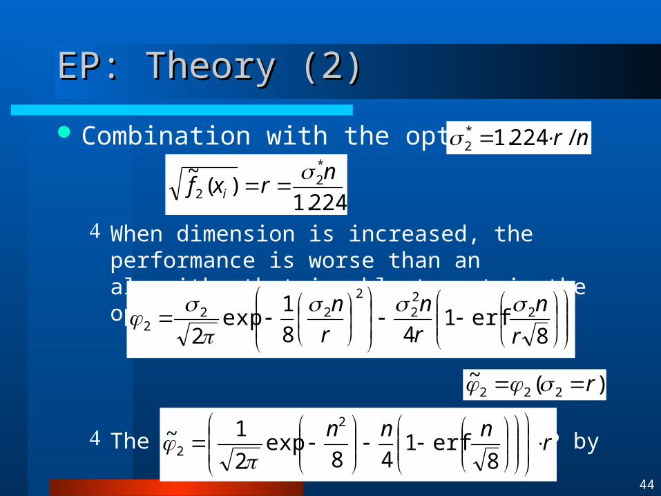
EP: Theory (2)EP: Theory (2)
Combination with the optimal SD
When dimension is increased, the performance is worse than an algorithm that is able to retain the opt. SD
The convergence rate of a (1+1)-EP by
224.1)(
~ *2
2
nrxf i
nr /224.1*2
8erf1
48
1exp
22
22
2
222
r
n
r
n
r
n
)(~222 r
rnnn
8erf1
48exp
2
1~2
2

45
Breeder GP: Motivation for GP Breeder GP: Motivation for GP TheoryTheory
In GP, parse trees of Lisp-like programs are used as chromosomes.
Performance of programs are evaluated by training error and the program size tends to grow as training error decreases.
Eventual goal of learning is to get small generalization error and the generalization error tends to increase as program size grows.
How to control the program growth?

46
Breeder GP: Breeder GP: MDL-Based MDL-Based Fitness FunctionFitness Function
)()|()|()( gi
giii ACADEDAFgF
)|( giADE
)( giAC
,
Training error of neural trees A for data set D
Structural complexity of neural trees A
Relative importance of each term

47
Breeder GP: Adaptive Occam Breeder GP: Adaptive Occam Method (Zhang et al., 1995)Method (Zhang et al., 1995)
otherwisetCtE
N
tEiftC
tEN
t
tCttEtF
bestbest
bestbest
best
iii
)()1(
1
)1()(
)1(
)(
)()()()(
2
2
Desired performance level in error
Training error of best progr. at gen t-1
Complexity of best progr. at gen. t
)1( tEbest
)(tCbest

48
Bayesian Evolutionary Computation (1/2)Bayesian Evolutionary Computation (1/2)
The best individual is defined as the most probable model of data D given the priori knowledge
The objective of evolutionary computation is defined to find the model A* that maximizes the posterior probability
Bayesian theorem is used to estimate P(A|D) from a population A(g) of individuals at each generation.
)(
)()|(
)()|(
)()|(
)()|(
)(
)()|()|(
gA
APADP
APADP
dAAPADP
APADP
DP
APADPDAP
A
)|(maxarg* DAPAA

49
Bayesian process: The BEAs attempt to explicitly estimate the posterior distribution of the individuals from their prior probability and likelihood, and then sample offspring from the distribution.
Bayesian Evolutionary Computation (2/2)Bayesian Evolutionary Computation (2/2)
[Zhang, 99]

50
Canonical BEACanonical BEA
(Initialize) Generate from the prior distribution P0(A). Set generation count t 0.
(P-step) Estimate posterior distribution Pt(A|D) of the individuals in At.
(V-step) Generate L variations by sampling from Pt(A|D).
(S-step) Select M individuals from A´ into based on Pt(A´i |D). Set the best individual .
(Loop) If the termination condition is met, then stop. Otherwise, set t t+1 and go to (P-step).
},,{ 001
0MAA A
},,{A 1 LAA
},,{A 111
tM
tt AA
51
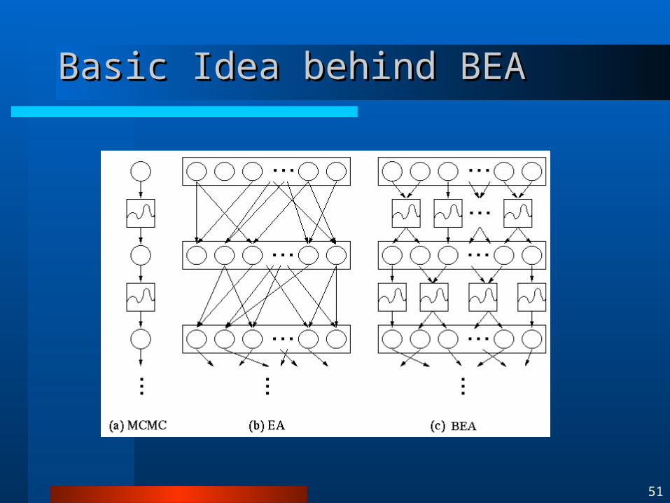
Basic Idea behind BEABasic Idea behind BEA

52
Evolving Neural Trees with BEAEvolving Neural Trees with BEA
Posterior probability of a neural tree A
)!3(
)exp(
2exp
2
1
2
))((exp
2
1
)()|(),|(
),(),|()()|()|(
3
1
1
21
21
2),(
k
w
fy
kPkPkDP
kpkDPAPADPDAP
k
k
jjk
N
cckcN
x
ww
ww
w

53
Features of EAsFeatures of EAs
Evolutionary techniques are good for problems that are ill-defined or difficult
Many different forms of representation Many different types of EA Leads to many different types of crossover,
mutation, etc. Some problems with convergence, efficiency However, they are able to solve a diverse range of
problems

54
Advantages of EAsAdvantages of EAs
Efficient investigation of large search spaces Quickly investigate a problem with a large number of
possible solutions
Problem independence Can be applied to many different problems
Best suited to difficult combinatorial problems

55
Disadvantages of EAsDisadvantages of EAs
No guarantee for finding optimal solutions with a finite amount of time: True for all global optimization methods.
No complete theoretical basis (yes). But much process is being made.
Parameter tuning is largely based on trial and error (genetic algorithms); solution: Self-adaptation (evolution strategies).
Often computationally expensive: Parallelism.

56
3. Applications3. Applications
57
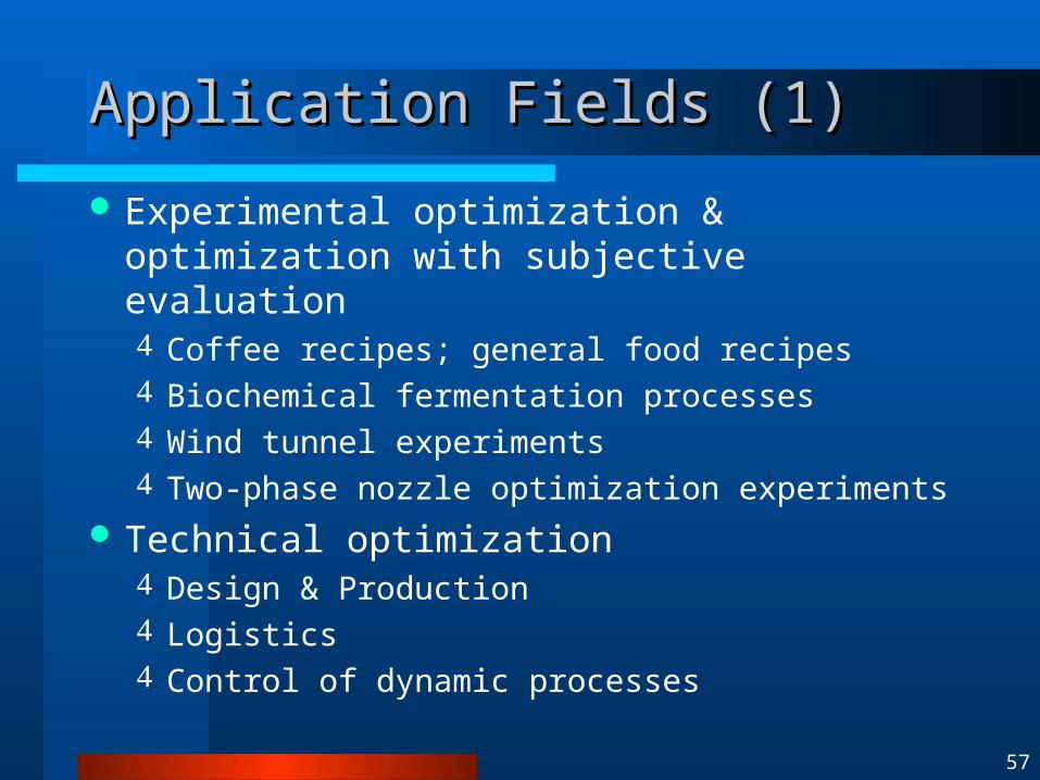
Application Fields (1)Application Fields (1)
Experimental optimization & optimization with subjective evaluation Coffee recipes; general food recipes Biochemical fermentation processes Wind tunnel experiments Two-phase nozzle optimization experiments
Technical optimization Design & Production Logistics Control of dynamic processes

58
Application Fields (2)Application Fields (2)
Structure optimization Structure & parameters of plants Connection structure & weights of neural nets Number of thicknesses of layers in multilayer
structures
Data Mining Clustering (number & centers of clusters) Fitting models to data Time series prediction

59
Application Fields (3)Application Fields (3)
Path Planning Traveling Salesman Problem
Robot Control Evolutionary Robotics Evolvable Hardware

60
Hot Water Flashing Nozzle (1)Hot Water Flashing Nozzle (1)
Start
Hot water entering Steam and droplet at exit
At throat: Mach 1 and onset of flashing
Application Example 1Application Example 1
Hans-Paul Schwefel performed the original experiments

61
Hot Water Flashing Nozzle (2)Hot Water Flashing Nozzle (2)Application Example 1Application Example 1

62
Minimal Weight Trust Layout Minimal Weight Trust Layout
LoadStart
922 kp
(LP minimum)
Optimum
738 kp
Application Example 2Application Example 2

63
Concrete Shell RoofConcrete Shell Roof
under own and outer load (snow and wind)
Height 1.34m
Spherical shapeOptimal shape
Half span 5.00m
Savings : 36% shell thickness 27% armation
max minOrthogonal bending strength
m
Application Example 3Application Example 3

64
Dipole Magnet Structure (1)Dipole Magnet Structure (1)
Mag
ne
tNS
yx
Mag
ne
tNS
yx
Mag
ne
tNS
yx
P1n
Fie
ld re
gio
n
of
inte
rest
y-
Ran
ge
Application Example 4Application Example 4

65
Dipole Magnet Structure (2)Dipole Magnet Structure (2)
Analysis of the magnetic field by Finite Element Analysis (FEM)
Minimize sum of squared deviations from the ideal
Individuals: Vectors of positions (y1, …, yn)
Middle: 9.8% better than upper graphic; bottom: 2.7% better
Application Example 4Application Example 4

66
Optical Multilayers (1)Optical Multilayers (1)
Goal: Find a filter structure such that the real reflection behavior matches the desired one as close as possible.
Filter layers; - Thicknesses - Materials
……..
Substrate (Glass)
Reflection
Wavele
ng
th
Desired
Current
Application Example 5Application Example 5
67
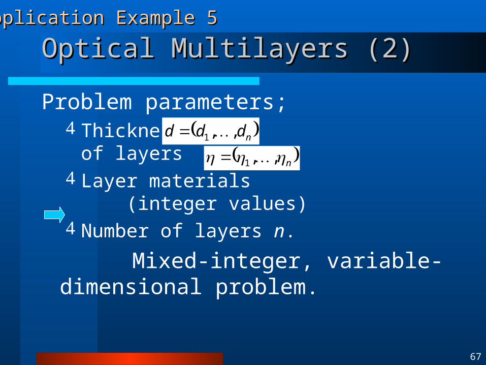
Optical Multilayers (2)Optical Multilayers (2)
Problem parameters; Thickness of layers Layer materials (integer values) Number of layers n.
Mixed-integer, variable-dimensional problem.
nddd ,,1
n ,,1
Application Example 5Application Example 5

68
Optical Multilayers (3)Optical Multilayers (3)
Objective function:
: Reflection of the actual filter for wavelength
Calculation according to matrix method.
: Desired reflection value
,,
dR
R~
dRdRdf
d
2~,,,
Application Example 5Application Example 5

69
Optical Multilayers (4)Optical Multilayers (4)
Example topology: Only layer thicknesses vary; n=2
Application Example 5Application Example 5

70
Optical Multilayers (5)Optical Multilayers (5)
Example structure:
Application Example 5Application Example 5

71
Optical Multilayers (6)Optical Multilayers (6)
Parallel evolutionary algorithm Per node: EA for mixed-integer representation Isolation and migration of best individuals Mutation of discrete variables: Fixed pm per population
Application Example 5Application Example 5

72
Circuit Design (1)Circuit Design (1)
Difficulty of automated circuit design: A vary hard problem
Exponential in the number of components More than 10300 circuits with a mere 20 components
An important problem Too few analog designers There is an “Egg-shell” of analog circuitry around almost all
digital circuits Analog circuits must be redesigned with each new generation of
process technology No existing automated techniques
In contrast with digital Existing analog techniques do only sizing of components, but do
not create the topology
Application Example 6Application Example 6

73
Circuit Design (2)Circuit Design (2)Application Example 6Application Example 6
OutIn
Developing Circuit
Development of a circuit with Genetic Programming
74
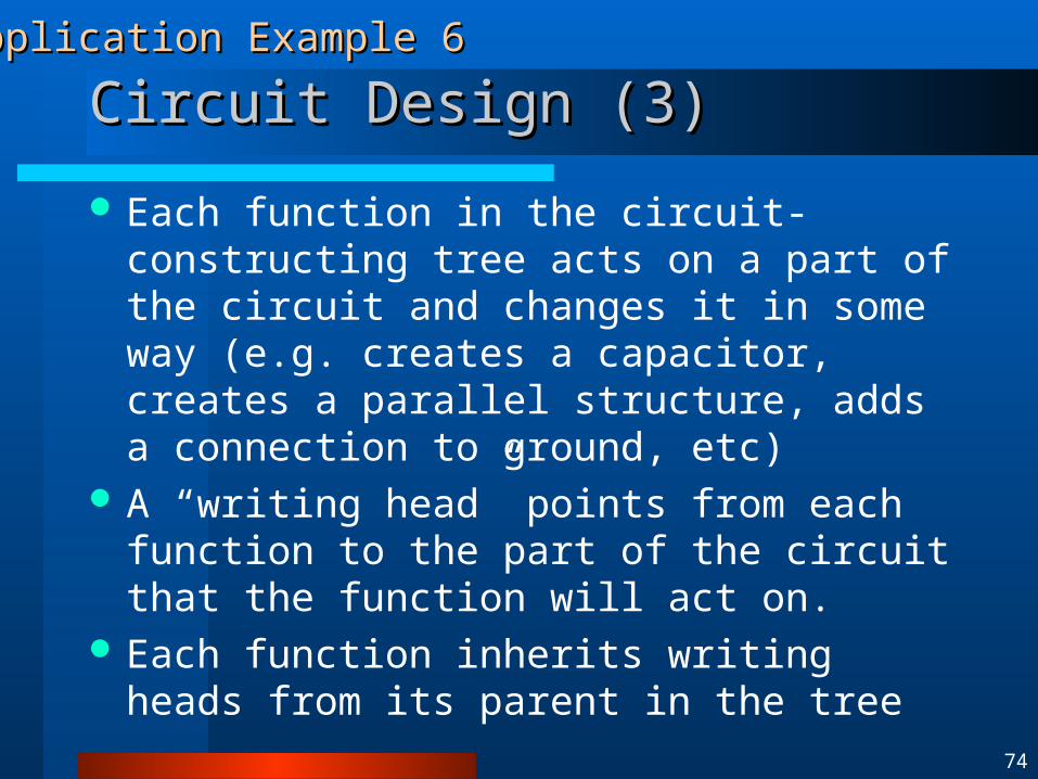
Circuit Design (3)Circuit Design (3)
Each function in the circuit-constructing tree acts on a part of the circuit and changes it in some way (e.g. creates a capacitor, creates a parallel structure, adds a connection to ground, etc)
A “writing head” points from each function to the part of the circuit that the function will act on.
Each function inherits writing heads from its parent in the tree
Application Example 6Application Example 6

75
Circuit Design (4)Circuit Design (4)
Example of circuit – constructing program tree
(LIST (C (-0.963 (- (- -0.875 – 0.113) 0.880)) (series (flip end) (series (flip end) (L –0.277 end) end) (L (- -0.640 0.749) (L –0.123 end)))) (flip (nop (L –0.657 end)))))
Application Example 6Application Example 6
LIST
C FLIP
NOP
-0.658 END
SERIES
SERIES
FLIP END
L
L
-0.277 ENDEND
L
- L
-0.658 -0.749 -0.658 END
-
-0.963 -
- -0.880
-0.875 -0.113
FLIP
END

76
Neural Network Design (1)Neural Network Design (1)
Introduction: EC for NNs Preprocessing of Training Data
Feature selection Training set optimization
Training of Network Weights Non-gradient search
Optimization of Network Architecture Topology adaptation Pruning unnecessary connections/units
Application Example 7Application Example 7

77
Neural Network Design (2)Neural Network Design (2)
Encoding Schemes for NNs
Bit-strings Properties of network structure are encoded as bit-
strings.
Rules Network configuration is specified by a graph-
generation grammar.
Trees Network is represented as “neural trees”.
Application Example 7Application Example 7

78
Neural Network Design (3)Neural Network Design (3)
Neural Tree ModelsNeural Tree Models Neural trees
Tree-structured neural networks Nonterminal nodes: Neural units Terminal nodes: Inputs Links: connection weights wij from j to i
Layer of node i: path length of the longest path to a terminal node of the substrees of i.
Type of Units Sigma unit: the sum of weighted inputs Pi unit: the product of weighted inputs Output of a neuron: sigmoid transfer function
},{ F},,,{ 21 nxxxT
j
jiji ywnet
j
jiji ywnet
inetii enetfy
1
1)(
Application Example 7Application Example 7

79
Neural Network Design (4)Neural Network Design (4)
S1
S2 P1 S4 S5
X2 X4 X1 S3 X3
X2 X1 X3 X2 X5
P2 X4 X4 S6
X1 X3
W11 W12 W13 W14
W21 W22 W31 W32 W33 W51 W52 W71 W72
W41 W42 W61 W62 W63 W81 W82
Application Example 7Application Example 7
Tree-Structured ModelTree-Structured Model

80
Neural Network Design (5)Neural Network Design (5)
Generate M Trees
Evaluate Fitness of Trees
Create L New Trees
Select Fitter Trees
Termination Condition? STOP
Posterior Distribution
Model Selection
Model Variation(Variation Operators)
Yes
No
Prior Distribution
Application Example 7Application Example 7
Evolving Neural Networks by BEAsEvolving Neural Networks by BEAs

81
Neural Network Design (6)Neural Network Design (6)
Structural Adaptation by Subtree Crossover Neuron type, topology, size and shape of networks are
adapted by crossover.
Neuron types and receptive fields are adapted by mutation. Connection weights are adapted by an EC-based stochastic
hill-climbing.
Application Example 7Application Example 7

82
Fuzzy System Design (1)Fuzzy System Design (1)
Fuzzy system comprises Fuzzy membership functions (MF) Rules
Task is to tailor the MF and rules to get best performance
Every change to MF affects the rules Every change to the rules affects the MF
Application Example 8Application Example 8

83
Fuzzy System Design (2)Fuzzy System Design (2)
Solution is to design MF and rules simultaneously Encode in chromosomes
Aarameters of the MF Associations and Certainty Factors in rules
Fitness is measured by performance of the Fuzzy System
Application Example 8Application Example 8

84
Fuzzy System Design (3)Fuzzy System Design (3)
Evolutionary Computation and Fuzzy Systems
Fuzzy Sets (Zadeh): Points have Memberships
Evolutionary Computation can be Used to Optimize Fuzzy Control Systems
Evolve Membership Functions/Rules
FUZZY MEMBERSHIP FOR “COOL”
Membership
0.0
1.0
0o 2.5o
Temperature (C)
Application Example 8Application Example 8

85
Fuzzy System Design (4)Fuzzy System Design (4)
NM=Negative Medium, NS=Negative Small, ZE=Zero, PS=Positive Small, PM=Positive Medium, _=No Entry
Defuzzification is Just Weighed Centroid Mutation Up/Down by One. Two-Point Xover on String Representing the 5x5
Metrix
Cart Centering and Fuzzy PartitionsFuzzy Control Strategy after 100 Gen.
Fm
x(v=x)
NM NS ZE PS PM
PM PM PM
PM
PM
PM
PM
PM
PM
NM
PM
NM NM NM
NM
NMNM
NS
NM NS ZE PS PM
NM
NS
ZE
PS
PM
x
v
Application Example 8Application Example 8
GA for Fuzzy Control of CartGA for Fuzzy Control of Cart
86
Data Mining (1)Data Mining (1)
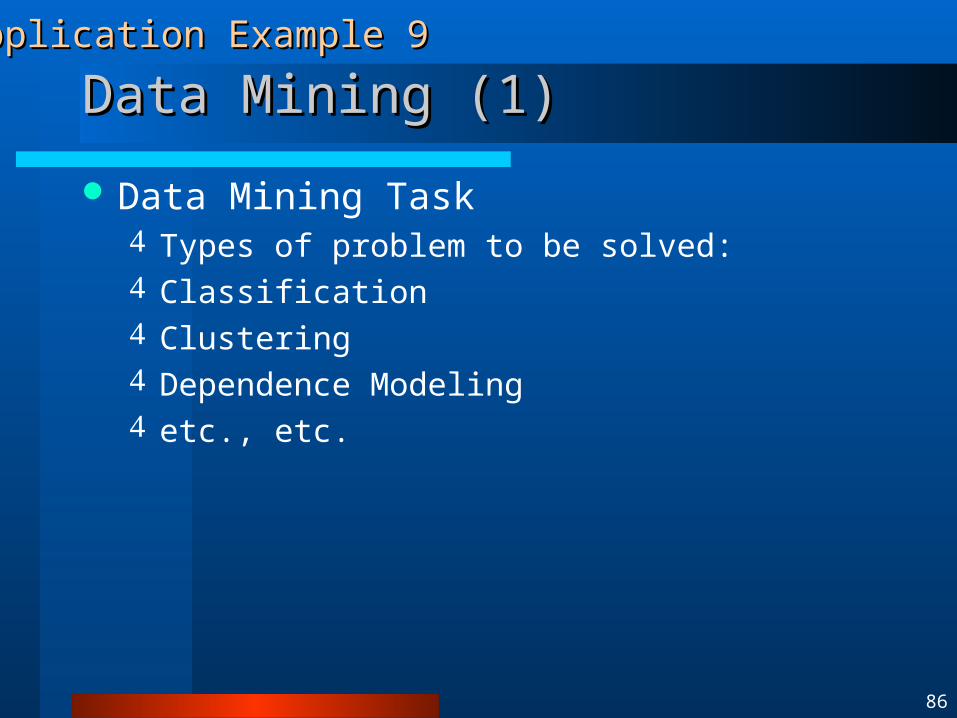
Data Mining Task Types of problem to be solved: Classification Clustering Dependence Modeling etc., etc.
Application Example 9Application Example 9

87
Data Mining (2)Data Mining (2)
Basic Ideas of GAs in Data Mining Candidate rules are represented as individuals of a
population Rule quality is computed by a fitness function Using task-specific knowledge
Application Example 9Application Example 9

88
Data Mining (3)Data Mining (3)
Classification with Genetic Algorithms Each individual represents a rule set
• i.e. an independent candidate solution
Each individual represents a single rule A set of individuals (or entire population) represents a
candidate solution (rule set)
Application Example 9Application Example 9

89
Data Mining (4)Data Mining (4)
Individual Representation In GABIL, an individual is a rule set, encoded as a bit string
[DeJong et al. 93] It uses k bits for the k values of a categorical attribute If all k bits of an attribute are set to 1 the attribute is not used by
the rule Goal attribute: Buy furniture Marital_status: Single/Married/Divorced House:Own/Rented/University Marital_status House Buy? The string 011 100 1 Represents the rule IF(Marital_status=M or D) and (House = 0) THEN (Buy furniture=y)
Application Example 9Application Example 9

90
Data Mining (5)Data Mining (5)
An individual is a variable-length string representing a set of fixed-length rules
rule 1 rule 2
011 100 1 101 110 0
Mutation: traditional bit inversion Crossover: corresponding crossover points in the
two parents must semantically match
Application Example 9Application Example 9

91
Information Retrieval (1)Information Retrieval (1)Text Data
Classification System
Information Filtering System
questionuser profile
feedback
answer
DB
LocationDate
DB Record
DB Template Filling& InformationExtraction System
Information FilteringInformation Extraction
filtered data
Text Classification
Preprocessing and Indexing
Application Example 10Application Example 10
92
Information Retrieval (2)Information Retrieval (2)
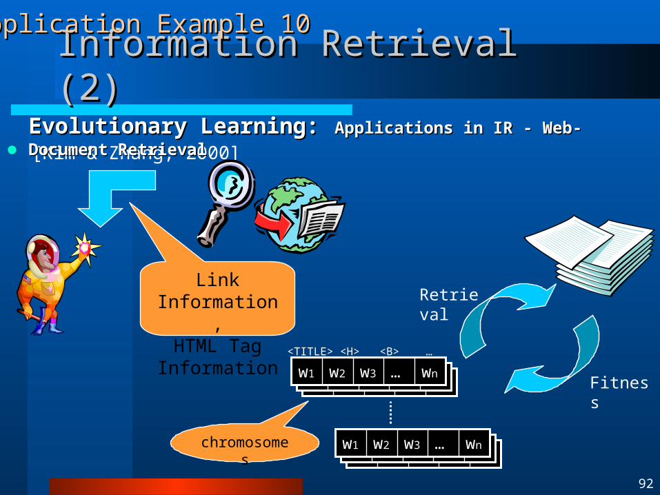
[Kim & Zhang, 2000]
Link Information,HTML Tag Information
chromosomes
<TITLE> <H> <B> … <A>
Retrieval
Fitness
wn…w3w2w1
wn…w3w2w1 wn…w3w2w1 wn…w3w2w1
wn…w3w2w1 wn…w3w2w1
Application Example 10Application Example 10
Evolutionary Learning:Evolutionary Learning: Applications in IR - Web-Document RetrievalApplications in IR - Web-Document Retrieval

93
Information Retrieval (3)Information Retrieval (3)
Crossover
Truncation selection
Mutation
yn…y3y2y1xn…x3x2x1
chromosome X chromosome Y
chromosome Z (offspring)
zi = (xi + yi ) / 2 w.p. Pc
chromosome X
chromosome X’
change value w.p. Pm
xn…x3x2x1
xn…x3x2x1zn…z3z2z1
Application Example 10Application Example 10
Evolutionary Learning: Evolutionary Learning: Applications in IR – Tag WeightingApplications in IR – Tag Weighting

94
Information Retrieval (4)Information Retrieval (4)
Datasets TREC-8 Web Track Data 2GB, 247491 web documents (WT2g) No. of training topics: 10, No. of test topics: 10
Results
Application Example 10Application Example 10
Evolutionary Learning : Evolutionary Learning : Applications in IR - Experimental ResultsApplications in IR - Experimental Results

95
Time Series Prediction (1)Time Series Prediction (1)Application Example 11Application Example 11
RawTime Series
RawTime Series
Prepro-cessingPrepro-cessing
EvolutionaryNeural Trees
(ENTs)
EvolutionaryNeural Trees
(ENTs)
CombiningNeural TreesCombining
Neural Trees
AutonomousModel Discovery
Combine Neural TreesOutputs
Prediction
[Zhang & Joung, 2000]

96
Time Series Prediction (2)Time Series Prediction (2) Experimental Setup for the far-infrared NH3
Laser
Design Paramenters Values Used
population size 200
max generation 50
crossover rate 0.95
mutation rate 0.1
no. of iterations 100
training set size 1000
test set size 1000
size of committee pool 10
no. of committee members 3
Application Example 11Application Example 11

97
Time Series Prediction (3)Time Series Prediction (3)
Experimental Result
0
0.1
0.2
0.3
0.4
0.5
0.6
0.7
0.8
0.9
1
1 201 401 601 801 1001 1201 1401 1601 1801 2001
t
x(t
)
0
0.1
0.2
0.3
0.4
0.5
0.6
0.7
0.8
0.9
1
0 200 400 600 800 1000 1200 1400 1600 1800 2000
t
x(t
)
Computed Approximation
Target Function
Application Example 11Application Example 11

98
Traveling Salesman Problem (1)Traveling Salesman Problem (1)
This is a minimization problem Given n cities, what is the shortest route to each
city, visiting each city exactly once Want to minimize total distance traveled Also must obey the “Visit Once” constraint
Application Example 12Application Example 12

99
Traveling Salesman Problem (2)Traveling Salesman Problem (2)
Encoding represents the order of cities to visit Candidates scored by total distance traveled
1
0
3
2 5
6
4
Application Example 12Application Example 12

100
Traveling Salesman Problem (3)Traveling Salesman Problem (3)
Traveling Salesman Problem (TSP) combinatorial optimization problems a salesman seeks the shortest tour through n cities NP-complete problem
Application Example 12Application Example 12

101
Traveling Salesman Problem (4)Traveling Salesman Problem (4)
Simple Example with the TSP The “house-call problem”
• Problem: Doctor must visit patients once and only once and return home in the shortest possible path
Difficulty: The number of possible routes increases faster than exponentially
• 10 patients = 191,440 possible routes
• 22 patients = 10,000,000,000,000,000,000,000
Application Example 12Application Example 12
102
Traveling Salesman Problem (5)Traveling Salesman Problem (5)
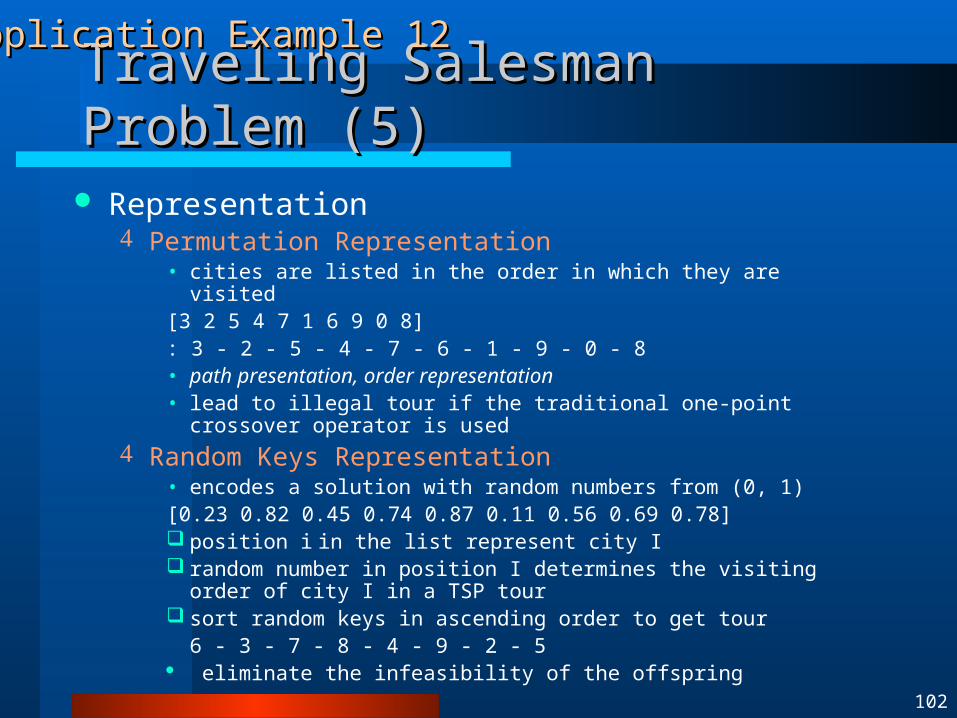
Representation Permutation Representation
• cities are listed in the order in which they are visited[3 2 5 4 7 1 6 9 0 8] : 3 - 2 - 5 - 4 - 7 - 6 - 1 - 9 - 0 - 8• path presentation, order representation• lead to illegal tour if the traditional one-point crossover operator is used
Random Keys Representation• encodes a solution with random numbers from (0, 1)[0.23 0.82 0.45 0.74 0.87 0.11 0.56 0.69 0.78] position i in the list represent city I random number in position I determines the visiting order of city I in a TSP
tour sort random keys in ascending order to get tour
6 - 3 - 7 - 8 - 4 - 9 - 2 - 5 eliminate the infeasibility of the offspring
Application Example 12Application Example 12

103
Cooperating Robots (1)Cooperating Robots (1)
What is Evolutionary Robotics? An attempt to create robots which evolve using various
evolutionary computational methods Evolve behaviors or competence modules implemented
in various manners: several languages, relay, neuro chips, FPGA’s, etc.
“Intelligence is emergent” Presently, limited to mostly evolution of robot’s control
software. However, some attempts to evolve hardware began.
GA and its variants used. Most current attempts center around {population size=50 ~ 500, generations = 50 ~ 500}
Application Example 13Application Example 13

104
Cooperating Robots (2)Cooperating Robots (2)
CLOSED
OPEN !!
Application Example 13Application Example 13
Industrial Robots Industrial Robots Autonomous Mobile RobotsAutonomous Mobile Robots

105
Cooperating Robots (3)Cooperating Robots (3)
Cooperating Autonomous Robots
Application Example 13Application Example 13

106
Cooperating Robots (4)Cooperating Robots (4)
Why Build Cooperating Robots? Increased scope for missions inherently
distributed in: • Space • Time • Functionality
Increased reliability, robustness (through redundancy)
Decreased task completion time (through parallelism)
Decreased cost (through simpler individual robot design)
Application Example 13Application Example 13

107
Cooperating Robots (5)Cooperating Robots (5) Cooperating Autonomous Robots: Application
domain Mining Construction Planetary exploration Automated manufacturing Search and rescue missions Cleanup of hazardous waste Industrial/household maintenance Nuclear power plant decommissioning Security, surveillance, and reconnaissance
Application Example 13Application Example 13
108
Co-evolving Soccer Softbots (1)Co-evolving Soccer Softbots (1)
At RoboCup there are two "leagues": the "real" robot league and the "virtual" softbot league
How do you do this with GP? GP breeding strategies: homogeneous and heterogeneous Decision of the basic set of function with which to evolve players Creation of an evaluation environment for our GP individuals
Application Example 14Application Example 14
Co-evolvingCo-evolving Soccer Softbots Soccer Softbots With Genetic With Genetic ProgrammingProgramming

109
Co-evolving Soccer Softbots (2)Co-evolving Soccer Softbots (2)
Initial Random Population
Application Example 14Application Example 14

110
Co-evolving Soccer Softbots (3)Co-evolving Soccer Softbots (3)
Kiddie Soccer
Application Example 14Application Example 14

111
Co-evolving Soccer Softbots (4)Co-evolving Soccer Softbots (4)
Learning to Block the Goal
Application Example 14Application Example 14

112
Co-evolving Soccer Softbots (5)Co-evolving Soccer Softbots (5)
Becoming Territorial
Application Example 14Application Example 14

113
Evolvable Hardware (1)Evolvable Hardware (1)
EVOLVABLE HARDWARE
HARDWARE IMPLEMENTATION OF EVOLVABLE SOFTWARE (i.e. GP)
Reconfigurable logic is too slow to make it worthwhile
Application Example 15Application Example 15

114
Evolvable Hardware (2)Evolvable Hardware (2)
FPGAs Bad, because they are designed for
conventional electronic design Good, because they can be abused and allow
the exploitation of the physics
FPMAs Field Programmable Matter Arrays
WHAT WE NEED
Application Example 15Application Example 15

115
Evolvable Hardware (3)Evolvable Hardware (3)
Can we, by evolving the voltages configure the material to carry out a useful function?
KEY REQUIREMENT
Removing the voltage must cause the material
to relax to its former state
wires Chemical substrate
A single piece of material
Region to which voltage may be applied
Application Example 15Application Example 15
What is a FPMA?What is a FPMA?

116
Evolvable Hardware (4)Evolvable Hardware (4)
XC6216 FPGA
Application Example 15Application Example 15

117
Evolvable Hardware (5)Evolvable Hardware (5)
Application Example 15Application Example 15
The Evolvable Hardware Robot Controller
The logic functions are evolved, and implemented in a RAM chip
A allows a signal to be either synchronised to a clock of evolved frequency, or passed straight through asynchronously, all under genetic control.
All evaluations performed using the REAL HARDWARE

118
Evolvable Hardware (6)Evolvable Hardware (6)Application Example 15Application Example 15

119
4. Current Issues4. Current Issues

120
Innovative Techniques for ECInnovative Techniques for EC
Effective Operators Novel Representation Exploration/Exploitation Population Sizing Niching Methods Dynamic Fitness Evaluation
Multi-objective Optimization Co-evolution Self-Adaptation EA/NN/Fuzzy Hybrids Distribution Estimation Algorithms Parallel Evolutionary Algorithms Molecular Evolutionary Computation

121
1000-Pentium Beowulf-Style 1000-Pentium Beowulf-Style Cluster Computer for Parallel GPCluster Computer for Parallel GP

122
Molecular Evolutionary Molecular Evolutionary ComputingComputing
011001101010001 ATGCTCGAAGCT

123
Applications of EAs Applications of EAs
Optimization Machine learning Data mining Intelligent Agents Bioinformatics Engineering Design Telecommunications Evolvable Hardware Evolutionary Robotics

124
5. References and URLs5. References and URLs

125
Journals & ConferencesJournals & Conferences
Journals: Evolutionary Computation (MIT Press) Trans. on Evolutionary Computation (IEEE) Genetic Programming & Evolvable Hardware
(Kluwer) Evolutionary Optimization
Conferences: Congress on Evolutionary Computation (CEC) Genetic and Evolutionary Computation Conference
(GECCO) Parallel Problem Solving from Nature (PPSN)

126
WWW ResourcesWWW Resources
• Genetic Programming Notebook• http://www.geneticprogramming.comsoftware, people, papers, tutorial, FAQs
• Hitch-Hiker’s Guide to Evolutionary Computation• http://alife.santafe.edu/~joke/encore/wwwFAQ for comp.ai.genetic
• Genetic Algorithms Archive• http://www.aic.nrl.navy.mil/galistRepository for GA related information, conferences, etc.
• EVONET European Network of Excellence on Evolutionary Comp. : http://www.dcs.napier.ac.uk/evonet

127
BooksBooks
• Bäck, Th., Evolutionary Algorithms in Theory and Practice, Oxford
University Press, New York, 1996.• Mitchell, M., An Introduction to Genetic Algorithms, MIT Press, Cambridge, MA, 1996.• Fogel, D., Evolutionary Computation: Toward a New Philosophy of Machine Intelligence, IEEE Press, NJ, 1995. • Schwefel, H-P., Evolution and Optimum Seeking, Wiley, New York, 1995.• Koza, J., Genetic Programming, MIT Press, Cambridge, MA, 1992.• Goldberg, D., Genetic Algorithms in Search and Optimization, Addison- Wesley, Reading, MA, 1989.• Holland, J., Adaptation in Natural and Artificial Systems, Univeristy of Michigan Press, Ann Arbor, 1975.• Rechenberg, I., Evolutionsstrategie: Optimierung technischer Systeme nach Prinzipien der biologischen Evolution, Frommann-Holzboog Verlag, Stuttgart, 1973. • Fogel, L.J., Owens, A.J, and Walsh, M.J., Artificial Intelligence through Simulated Evolution, John Wiley, NY, 1966.

For more information:For more information:
http://scai.snu.ac.kr/http://scai.snu.ac.kr/
Recommended
![[PPT]슬라이드 제목 없음 - 한국CM협회에 오신걸 환영합니다. · Web viewSOC 민간투자사업의 추진전략 2003. 3. 11 김 탁 경 출자자의 의무사항 설정](https://img.pdfslide.net/doc/110x75/5aafc22b7f8b9aa8438db7bb/ppt-cm-viewsoc.jpg)


![교보악사 Tomorrow 장기우량 증권투자신탁 K-1 · 2019. 10. 2. · 1 교보악사 Tomorrow 장기우량 증권투자신탁 K-1호(채권) [신 탁 계 약 서] 교보악사](https://img.pdfslide.net/doc/110x75/5fc0d1af71792a47b2694c80/ee-tomorrow-ee-eoef-k-1-2019-10-2-1-ee.jpg)