Executing Robust Design
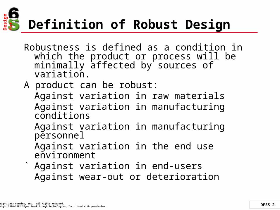
Definition of Robust Design
Robustness is defined as a condition in which the product or process will be minimally affected by sources of variation.
A product can be robust:Against variation in raw materialsAgainst variation in manufacturing conditionsAgainst variation in manufacturing personnelAgainst variation in the end use environment
` Against variation in end-usersAgainst wear-out or deterioration
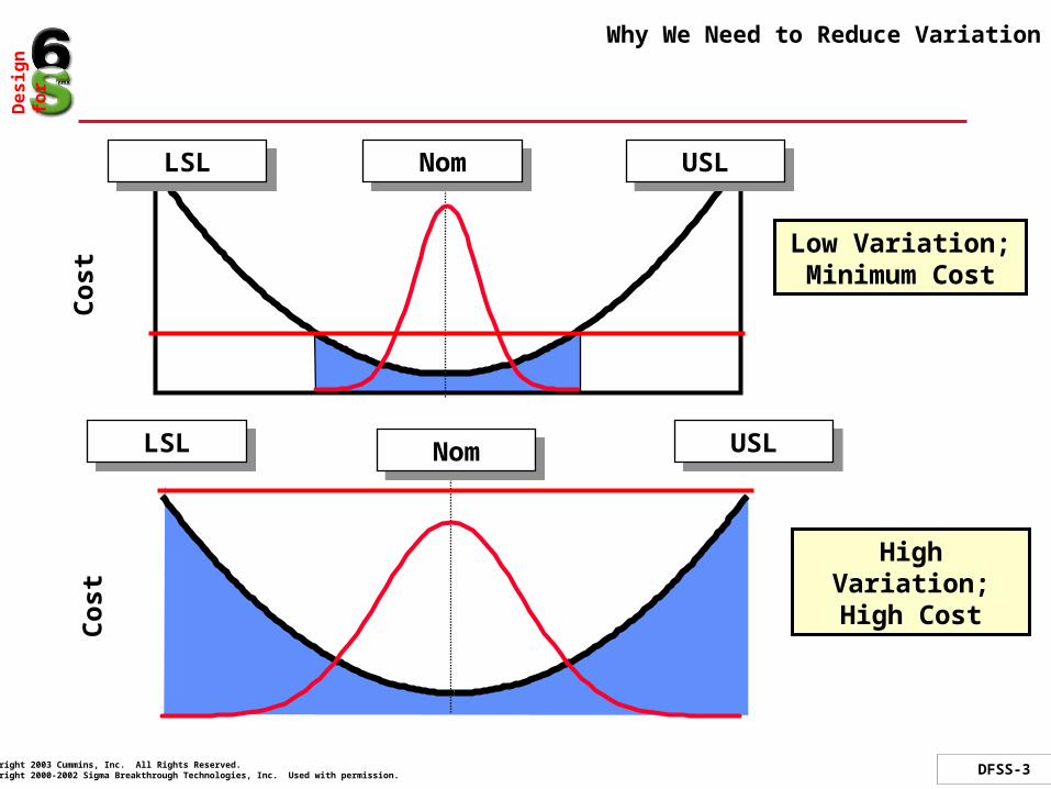
Why We Need to Reduce Variation
Cos
t
Low Variation;Minimum Cost
LSLLSL USLUSLNomNom
Cos
t
High Variation;High Cost
LSLLSL USLUSLNomNom
Purpose of this Module
To introduce a variation improvement investigation strategy– Can noise factors be manipulated?
To provide the MINITAB steps to design, execute, and analyze a variability response experiment
To provide the MINITAB steps to optimize a design for both mean and variation effects

Objectives of this Module
At the end of this module, participants will be able to :
Identify possible variation effects from residual plots Create a variability response from replicates Identify possible mean and variance adjustment
factors from noise-factor interaction plots Use the MINITAB Response Optimizer to achieve a
process on target with minimum variation
Strategies to Detect Variation Effects
Passive Approach– Noise factors are NOT included, manipulated or controlled in
the experimental design– Possible variation effects are identified through analysis of
the variability of replicates from an experimental design
Active Approach– Noise factors ARE included in the experimental design in
order to force variability to occur– Analysis is similar to the passive approach
The Passive Approach
A factorial experiment is performed using Control factors. Noise factors are not explicitly manipulated nor is an attempt made to control them during the course of the experiment.
Pros– Simple extension of standard experimental techniques– Does not require explicit identification of noise factors
Cons– Requires larger number of replicates than would typically be
required to determine mean effects– Requires “true” randomization and replication– Requires that noise factors be “noisy” during the execution
of the experiment
How to ensure that noise is noisy?
Let excluded factors vary Compare noise factor variations prior to and within
DOE– Monitor noise factor levels during normal process conditions– Monitor noise factor variation during course of experiment– Compare before/during levels
Run DOE over a longer period of time with :– More replicates– Full randomization
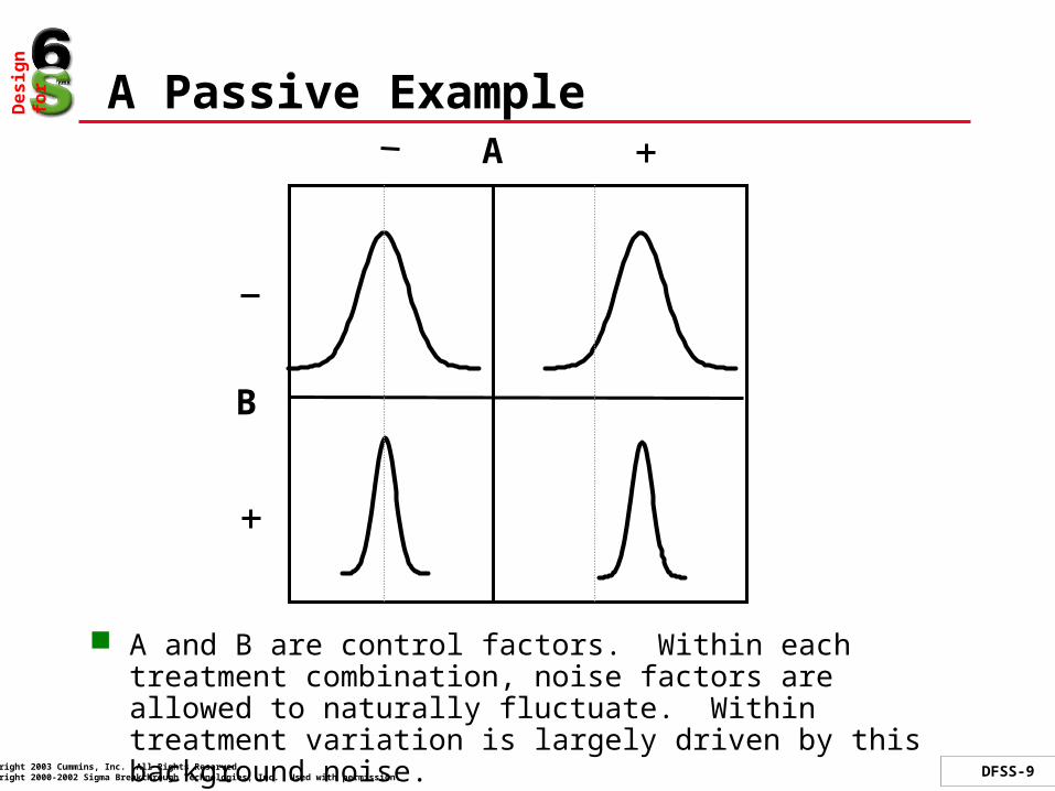
A Passive Example
A and B are control factors. Within each treatment combination, noise factors are allowed to naturally fluctuate. Within treatment variation is largely driven by this background noise.
A
B
Example output from a Passive Design
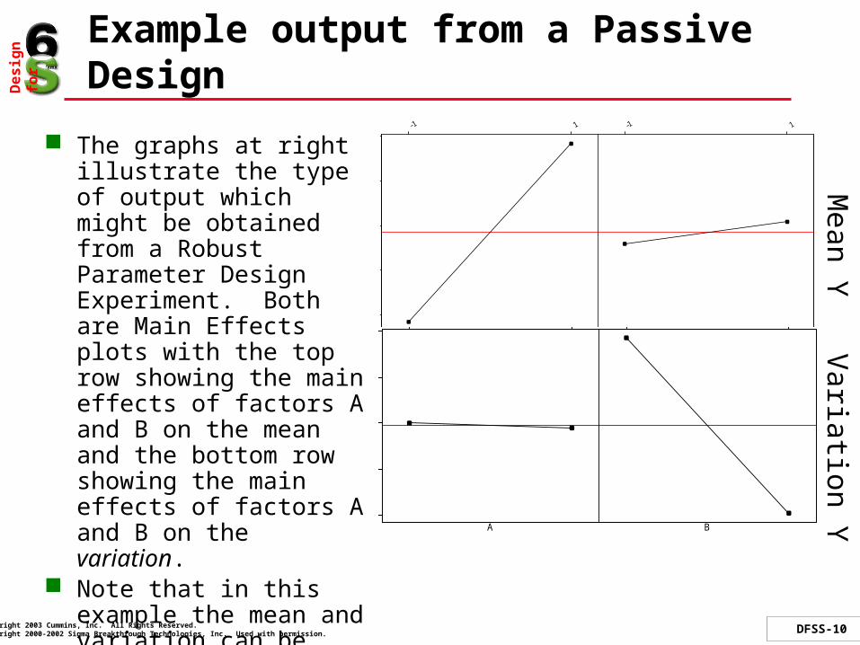
The graphs at right illustrate the type of output which might be obtained from a Robust Parameter Design Experiment. Both are Main Effects plots with the top row showing the main effects of factors A and B on the mean and the bottom row showing the main effects of factors A and B on the variation.
Note that in this example the mean and variation can be adjusted independently of each other!
BA
6.4
5.4
4.4
3.4
2.4
Mea
n
Mean Y
BA
0.6
0.4
0.2
0.0
-0.2
LogV
aria
nce
Variation Y

The Models
Our objective in performing a designed experiment is to develop a transfer function between the factors (X’s) and the Y. Thus far, we have only addressed the mean of Y.
Now we must also consider the variability of Y
If our experiments are successful at identifying a variation effect, we now have an opportunity to simultaneously optimize both equations!
211222110
2xxcxcxccs y
211222110 xxbxbxbby

Example: A Passive Noise Experiment
A design engineer has evaluated the output performance of a circuit design and performed an initial capability analysis of this design to determine if there is a problem with the mean and/or the variability.
Stat > Quality Tools > Capability Analysis > Normal
Y = Y1Initial; Lower Spec = 58; Upper Spec = 62
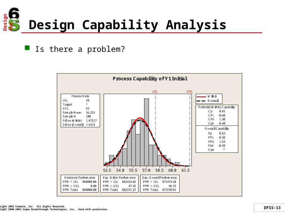
Design Capability Analysis
Is there a problem?
61.560.058.557.055.554.052.5
LSL USLProcess Data
Sample N 100StDev(Within) 1.47217StDev(Overall) 1.5414
LSL 58Target *USL 62Sample Mean 56.253
Potential (Within) Capability
Overall Capability
Pp 0.43PPL -0.38PPU 1.24Ppk -0.38Cpm
Cp
*
0.45CPL -0.40CPU 1.30Cpk -0.40
Observed PerformancePPM < LSL 860000.00PPM > USL 0.00PPM Total 860000.00
Exp. Within PerformancePPM < LSL 882324.02PPM > USL 47.35PPM Total 882371.37
Exp. Overall PerformancePPM < LSL 871474.48PPM > USL 96.33PPM Total 871570.81
WithinOverall
Process Capability of Y1Initial
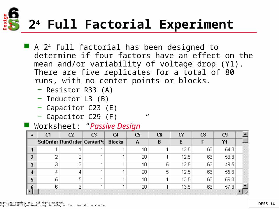
24 Full Factorial Experiment
A 24 full factorial has been designed to determine if four factors have an effect on the mean and/or variability of voltage drop (Y1). There are five replicates for a total of 80 runs, with no center points or blocks.– Resistor R33 (A)– Inductor L3 (B)– Capacitor C23 (E) – Capacitor C29 (F)
Worksheet: “Passive Design”

Passive Analysis Roadmap - Part 1(for Mean Only)
Analyze the response of interest– Factorial Plots (Main Effects, Interaction)– Statistical Results (ANOVA table and p-values)– Residual Plots by factor
Reduce model using statistical results
Use the residuals plot to evaluate potential existence of variation effects– If residuals plot indicates a possible variation effect, go to
Passive Analysis Roadmap - Part 2

Interaction Plot
Based on the interaction plot, a few of the interactions may be significant. Check the statistical output for verification.
Stat > DOE > Factorial > Factorial Plots > Interaction Plot
A
E
F
B
51 13.512.5 6963
60.0
57.5
55.0
60.0
57.5
55.0
60.0
57.5
55.0
A1020
B15
E12.513.5
Interaction Plot (data means) for Y1

Main Effects Plot
The main effects plot indicates that factors B and E have the largest effects. Factor A also has a moderate positive effect. Factor F does not seem to be important. Let’s look at the results.
Stat > DOE > Factorial > Factorial Plots > Main Effects Plot
Mean o
f Y1
2010
58
57
56
55
5451
13.512.5
58
57
56
55
546963
A B
E F
Main Effects Plot (data means) for Y1
Factorial Analysis
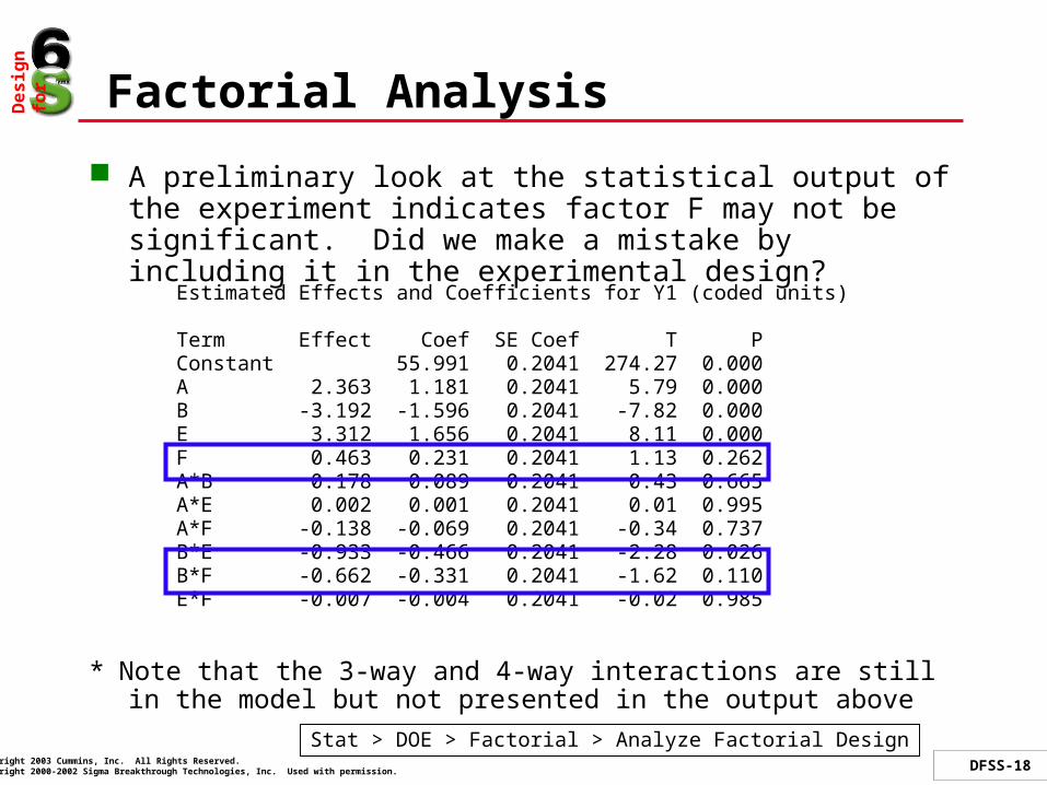
A preliminary look at the statistical output of the experiment indicates factor F may not be significant. Did we make a mistake by including it in the experimental design?
* Note that the 3-way and 4-way interactions are still in the model but not presented in the output above
Stat > DOE > Factorial > Analyze Factorial Design
Estimated Effects and Coefficients for Y1 (coded units)
Term Effect Coef SE Coef T PConstant 55.991 0.2041 274.27 0.000A 2.363 1.181 0.2041 5.79 0.000B -3.192 -1.596 0.2041 -7.82 0.000E 3.312 1.656 0.2041 8.11 0.000F 0.463 0.231 0.2041 1.13 0.262A*B 0.178 0.089 0.2041 0.43 0.665A*E 0.002 0.001 0.2041 0.01 0.995A*F -0.138 -0.069 0.2041 -0.34 0.737B*E -0.933 -0.466 0.2041 -2.28 0.026B*F -0.662 -0.331 0.2041 -1.62 0.110E*F -0.007 -0.004 0.2041 -0.02 0.985
Reduce Model to Significant Terms
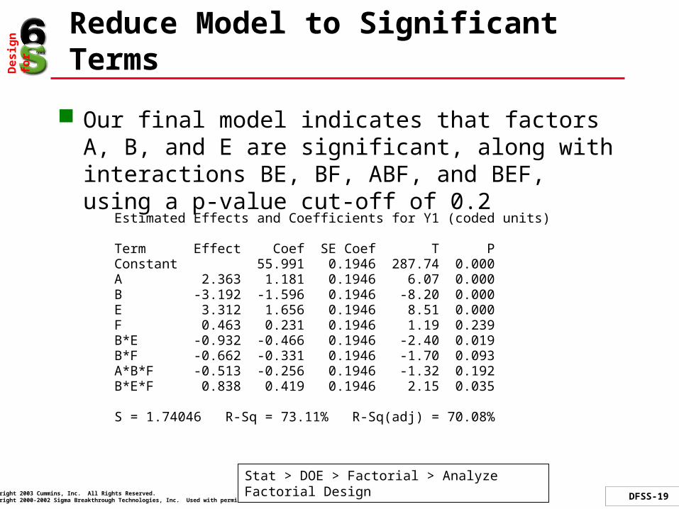
Our final model indicates that factors A, B, and E are significant, along with interactions BE, BF, ABF, and BEF, using a p-value cut-off of 0.2
Estimated Effects and Coefficients for Y1 (coded units)
Term Effect Coef SE Coef T PConstant 55.991 0.1946 287.74 0.000A 2.363 1.181 0.1946 6.07 0.000B -3.192 -1.596 0.1946 -8.20 0.000E 3.312 1.656 0.1946 8.51 0.000F 0.463 0.231 0.1946 1.19 0.239B*E -0.932 -0.466 0.1946 -2.40 0.019B*F -0.662 -0.331 0.1946 -1.70 0.093A*B*F -0.513 -0.256 0.1946 -1.32 0.192B*E*F 0.838 0.419 0.1946 2.15 0.035
S = 1.74046 R-Sq = 73.11% R-Sq(adj) = 70.08%
Stat > DOE > Factorial > Analyze Factorial Design

The Role of Residual Plots in RD
In Robust Parameter Design, the residual plots can show the possibility for a variation effect
Remember from ANOVA and Regression, we stated one of the assumptions on the residuals was constant variance and we checked this via plots
Stat > DOE > Factorial > Analyze Factorial Design
Choose Graphs > Residuals vs Variables > A B E F
What Next?
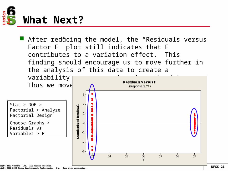
After reducing the model, the “Residuals versus Factor F” plot still indicates that F contributes to a variation effect. This finding should encourage us to move further in the analysis of this data to create a variability response and analyze the data. Thus we move on to Part 2 of the roadmap.
F
Sta
ndard
ized R
esi
dual
69686766656463
3
2
1
0
-1
-2
-3
Residuals Versus F(response is Y1)
Stat > DOE > Factorial > Analyze Factorial Design
Choose Graphs > Residuals vs Variables > F
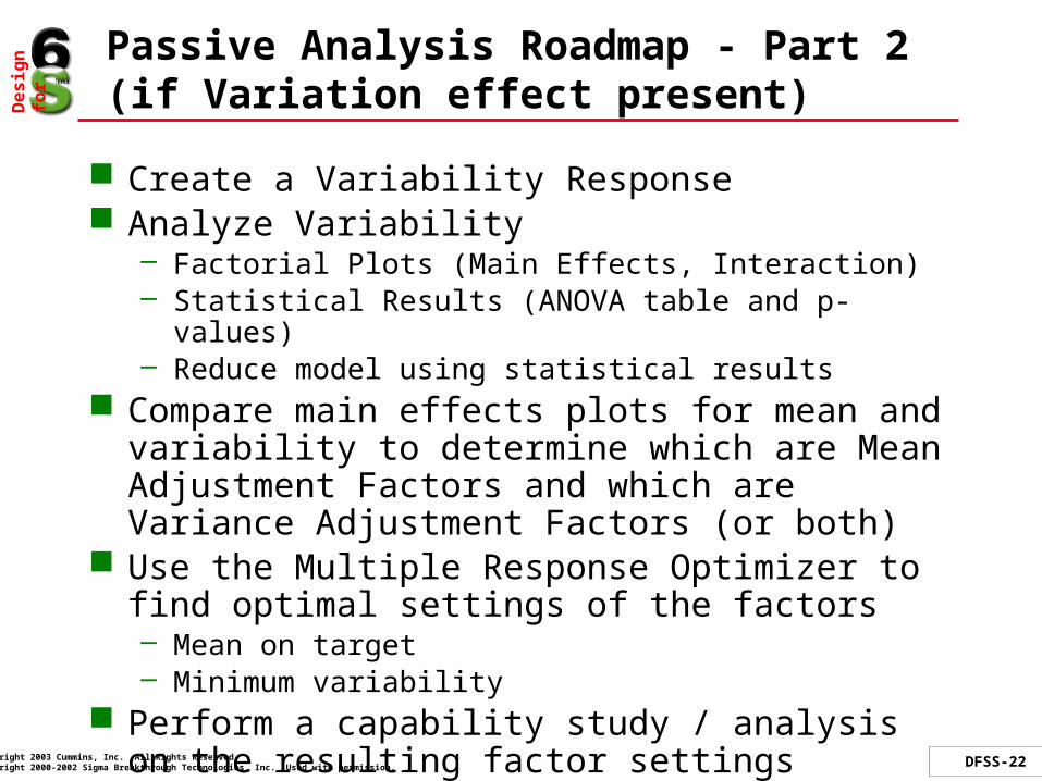
Create a Variability Response Analyze Variability
– Factorial Plots (Main Effects, Interaction)– Statistical Results (ANOVA table and p-values)– Reduce model using statistical results
Compare main effects plots for mean and variability to determine which are Mean Adjustment Factors and which are Variance Adjustment Factors (or both)
Use the Multiple Response Optimizer to find optimal settings of the factors– Mean on target– Minimum variability
Perform a capability study / analysis on the resulting factor settings
Passive Analysis Roadmap - Part 2(if Variation effect present)
Create a Variability Response
We are now going to use the replications to make a new response in order to model the variability. Once we have modeled the variability, we can use the MINITAB Response Optimizer to find the settings of the control factors that will put Y on target with minimum variation.
MINITAB makes this easy with a pre-processing of the responses in preparation for a variability analysis
You will see that MINITAB will use the standard deviation as the measure of variability, rather than the variance– the results are equivalent
Uses Natural Log (Standard Dev of Y)
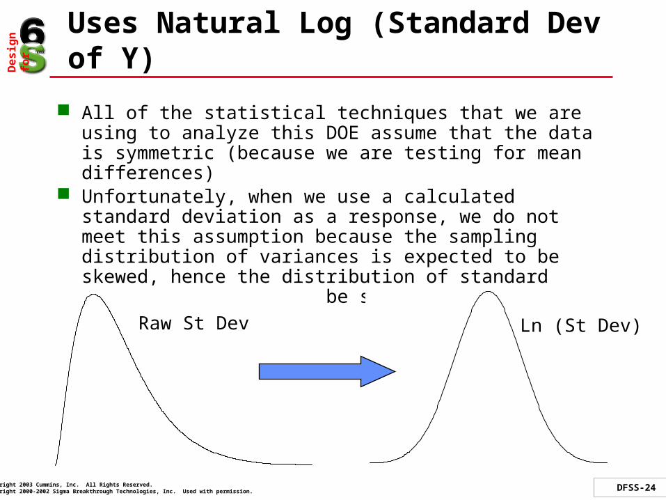
All of the statistical techniques that we are using to analyze this DOE assume that the data is symmetric (because we are testing for mean differences)
Unfortunately, when we use a calculated standard deviation as a response, we do not meet this assumption because the sampling distribution of variances is expected to be skewed, hence the distribution of standard deviations would also be skewed
Raw St Dev Ln (St Dev)

Create a Variability Response
Stat > DOE > Factorial > Pre-Process Responses for Analyze Variability
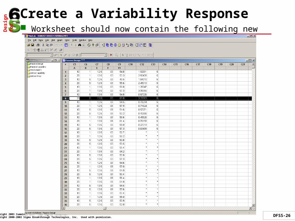
Create a Variability Response Worksheet should now contain the following new columns
Analyze the Variability
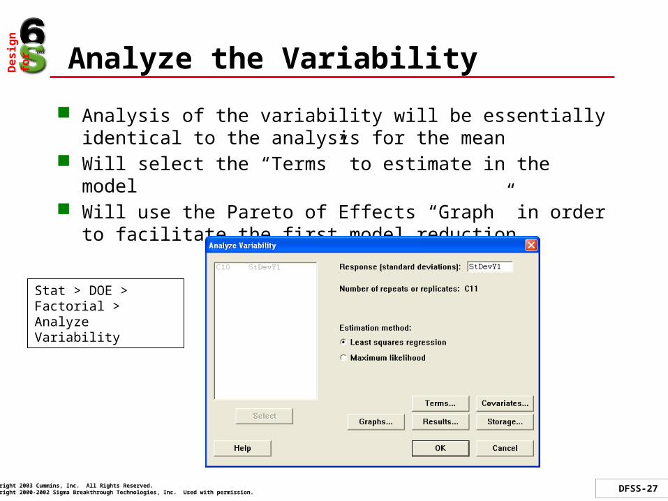
Analysis of the variability will be essentially identical to the analysis for the mean
Will select the “Terms” to estimate in the model Will use the Pareto of Effects “Graph” in order to facilitate the
first model reduction
Stat > DOE > Factorial > Analyze Variability
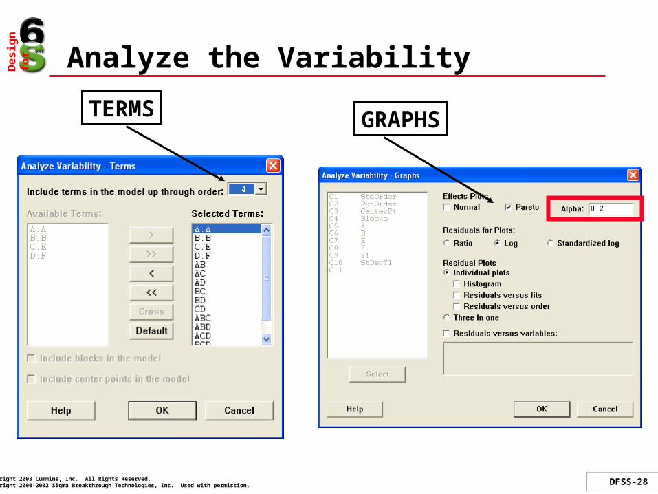
Analyze the Variability
TERMS GRAPHS

Pareto Chart of the Effects
Because we don’t have any degrees of freedom for error, we must look at the Pareto of effects to decide which term to drop into the error and begin to reduce the model
Term
Effect
ABD
BC
CD
ACD
AB
ABCD
BD
BCD
ABC
C
AD
B
AC
A
D
1.41.21.00.80.60.40.20.0
0.130Factor
F
NameA AB BC ED
Pareto Chart of the Effects(Response is natural log of StDevY1, Alpha = 0.20)
Lenth's PSE = 0.0878313
Drop ABD interaction first

Final Model for ln StDevY1
Once the insignificant terms have been eliminated using a p-value cut-off of 0.2, the reduced model is shown below
Regression Estimated Effects and Coefficients for Natural Log of StDevY1 (coded units)
RatioTerm Effect Effect Coef SE Coef T PConstant 0.0747 0.01013 7.38 0.002A 0.5139 1.6718 0.2569 0.01013 25.37 0.000B -0.2953 0.7443 -0.1477 0.01013 -14.58 0.000E -0.1521 0.8589 -0.0760 0.01013 -7.51 0.002F -1.3384 0.2623 -0.6692 0.01013 -66.08 0.000A*B 0.0371 1.0378 0.0185 0.01013 1.83 0.141A*E 0.4451 1.5606 0.2225 0.01013 21.98 0.000A*F -0.2573 0.7731 -0.1287 0.01013 -12.71 0.000B*F -0.0781 0.9249 -0.0390 0.01013 -3.86 0.018A*B*E 0.1323 1.1414 0.0661 0.01013 6.53 0.003B*E*F 0.0850 1.0887 0.0425 0.01013 4.20 0.014A*B*E*F 0.0390 1.0398 0.0195 0.01013 1.93 0.126
R-Sq = 99.93% R-Sq(adj) = 99.75%

Interaction Plot for StDevY1
The interaction plot indicates a moderately strong interaction between factors A & E and A & F
Stat > DOE > Factorial > Factorial Plots > Interaction Plot
A
E
F
B
51 13.512.5 6963
3
2
1
3
2
1
3
2
1
A1020
B15
E12.513.5
Interaction Plot (data means) for StDevY1
Where should factors A, B, E and F be set in order to minimize the variability in voltage drop, Y1?

Main Effects Plot for StDevY1 Factor F has the largest effect on the variability. Increasing F should
reduce variability. But what did the interaction plot show? Factor A is the next strongest. Set A = 10. What did the interaction plot
show? Factors B and E are weak but what did the interaction plot show?
Mean o
f StD
evY1
2010
2.5
2.0
1.5
1.0
0.551
13.512.5
2.5
2.0
1.5
1.0
0.56963
A B
E F
Main Effects Plot (data means) for StDevY1
Stat > DOE > Factorial > Factorial Plots > Main Effects Plot
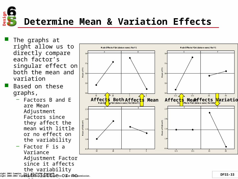
Determine Mean & Variation Effects
The graphs at right allow us to directly compare each factor’s singular effect on both the mean and variation
Based on these graphs,– Factors B and E are
Mean Adjustment Factors since they affect the mean with little or no effect on the variability
– Factor F is a Variance Adjustment Factor since it affects the variability with little or no effect on the mean
– Factor A appears to affect both mean and variability
Mea
n o
f Y
1
2010
58
57
56
55
54
51
A B
Mea
n o
f Y
1
13.512.5
58
57
56
55
54
6963
E F
Me
an
of
StD
evY
1
2010
2.5
2.0
1.5
1.0
0.551
A B
Mea
n o
f StD
evY
1
13.512.5
2.5
2.0
1.5
1.0
0.5
6963
E F
Main Effects Plot (data means) for Y1 Main Effects Plot (data means) for Y1
Main Effects Plot (data means) for StDevY1 Main Effects Plot (data means) for StDevY1Affects Both Affects Mean Affects Mean Affects Variation

Quality Check: Status of Your Models
Use the “Show Design” icon to check on the status of the analysis. You should make sure that the correct model has been fit for each response that you intend to specify in the response optimizer.
As shown in this window, models have been fit for both the Y1 and StDevY1 responses
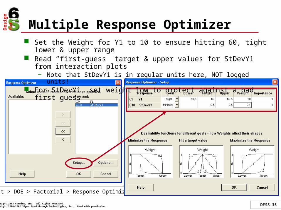
Multiple Response Optimizer
Stat > DOE > Factorial > Response Optimizer
Set the Weight for Y1 to 10 to ensure hitting 60, tight lower & upper range Read “first-guess” target & upper values for StDevY1 from interaction plots
– Note that StDevY1 is in regular units here, NOT logged units! For StDevY1, set weight low to protect against a bad first guess
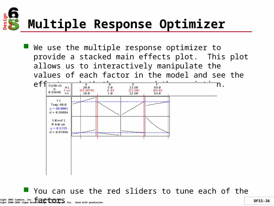
Multiple Response Optimizer
We use the multiple response optimizer to provide a stacked main effects plot. This plot allows us to interactively manipulate the values of each factor in the model and see the effect on both the mean and the variation.
You can use the red sliders to tune each of the factors
Hi
Lo0.93698D
Optimal
Cur
d = 0.87896
MinimumStDevY1
d = 0.99884
Targ: 60.0Y1
y = 0.5725
y = 60.0001
63.0
69.0
12.50
13.50
1.0
5.0
10.0
20.0B E FA
[13.4878] [1.0] [13.50] [69.0]
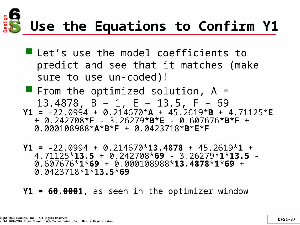
Use the Equations to Confirm Y1
Let’s use the model coefficients to predict and see that it matches (make sure to use un-coded)!
From the optimized solution, A = 13.4878, B = 1, E = 13.5, F = 69
Y1 = -22.0994 + 0.214670*A + 45.2619*B + 4.71125*E + 0.242708*F - 3.26279*B*E - 0.607676*B*F + 0.000108988*A*B*F + 0.0423718*B*E*F
Y1 = -22.0994 + 0.214670*13.4878 + 45.2619*1 + 4.71125*13.5 + 0.242708*69 - 3.26279*1*13.5 -0.607676*1*69 + 0.000108988*13.4878*1*69 + 0.0423718*1*13.5*69
Y1 = 60.0001, as seen in the optimizer window
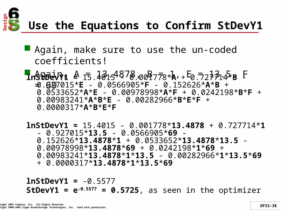
Use the Equations to Confirm StDevY1
Again, make sure to use the un-coded coefficients! Again, A = 13.4878, B = 1, E = 13.5, F = 69
lnStDevY1 = 15.4015 - 0.001778*A + 0.727714*B - 0.927015*E - 0.0566905*F - 0.152626*A*B + 0.0533652*A*E - 0.00978998*A*F + 0.0242198*B*F + 0.00983241*A*B*E - 0.00282966*B*E*F + 0.0000317*A*B*E*F
lnStDevY1 = 15.4015 - 0.001778*13.4878 + 0.727714*1 - 0.927015*13.5 - 0.0566905*69 - 0.152626*13.4878*1 + 0.0533652*13.4878*13.5 - 0.00978998*13.4878*69 + 0.0242198*1*69 + 0.00983241*13.4878*1*13.5 - 0.00282966*1*13.5*69 + 0.0000317*13.4878*1*13.5*69
lnStDevY1 = -0.5577StDevY1 = e-0.5577 = 0.5725, as seen in the optimizer

Final Design Capability Analysis Did we achieve our objectives?
61.6061.0560.5059.9559.4058.8558.30
LSL USLProcess Data
Sample N 100StDev(Within) 0.120084StDev(Overall) 0.115955
LSL 58Target *USL 62Sample Mean 60.3183
Potential (Within) Capability
Overall Capability
Pp 5.75PPL 6.66PPU 4.83Ppk 4.83Cpm
Cp
*
5.55CPL 6.44CPU 4.67Cpk 4.67
Observed PerformancePPM < LSL 0.00PPM > USL 0.00PPM Total 0.00
Exp. Within PerformancePPM < LSL 0.00PPM > USL 0.00PPM Total 0.00
Exp. Overall PerformancePPM < LSL 0.00PPM > USL 0.00PPM Total 0.00
WithinOverall
Process Capability of Y1Final
worksheet “passive capability”
Stat > Quality Tools > Capability Analysis > Normal
Y = Y1Final; Lower Spec = 58; Upper Spec = 62

Remember the Two Strategies?
We just reviewed the Passive Approach– Noise factors are NOT included, manipulated or controlled in
the experimental design– We analyzed the variability of replicates from an
experimental design
Now we will look at the Active Approach– Noise factors ARE included in the experimental design in
order to force variability to occur– We will see that the analysis is similar to the passive
approach

The Active Approach
A factorial experiment is performed using Control AND Noise factors in the same experiment. Analysis can be performed by characterizing Control*Noise interactions only or by moving forward to analyze the variability by dropping the noise factors into the error term.
Pros– Simple extension of standard experimental techniques– Guarantees noise in the Noise factors– Provides for flexibility in analysis methods– Can allow for reduced replication
Cons– Requires ability to manipulate and control Noise factors– Optimal designs for minimization of unneeded effects (noise by
noise interactions) can be difficult to create
3 control factors 1 noise factor 24 full factorial design
Two Approaches to Analysis– Use only interpretation of interaction plots to choose settings
of the control factors to minimize effect of noise– Model the variability by dropping the noise factors into the
error and analyze like the passive approach
Example: An Active Noise Experiment
Active Analysis Roadmap – Plots Only
Create and execute with noise included as a factor Analyze the response of interest
– Factorial Plots (Main Effects, Interaction)– Statistical Results (ANOVA table and p-values)– Reduce model using statistical results
Review Interactions Plot– Interpret the interaction plots to look for evidence of variation effects
Review Main Effects Plot (if applicable) Use the Multiple Response Optimizer to find the optimal settings
of the factors such that the mean is on target– Will force in settings obtained from the interaction plots
Perform a capability study / analysis on the resulting factor settings
Example: An Active Noise Experiment
An engineer is interested in improving the stability and robustness of a filtration product
Review the capability of the current performance to determine the opportunity to apply robust design techniques
Stat > Quality Tools > Capability Analysis > Normal
Y = Y4Initial; Lower Spec = 60; Upper Spec = 80
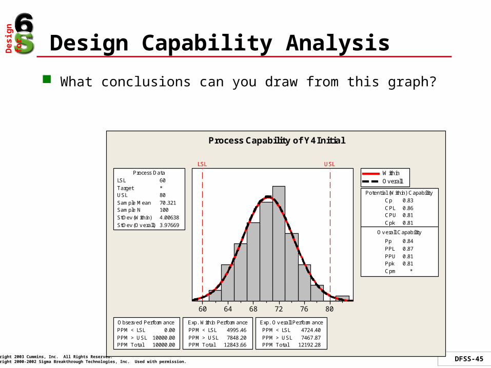
Design Capability Analysis
What conclusions can you draw from this graph?
807672686460
LSL USLProcess Data
Sample N 100StDev(Within) 4.00638StDev(Overall) 3.97669
LSL 60Target *USL 80Sample Mean 70.321
Potential (Within) Capability
Overall Capability
Pp 0.84PPL 0.87PPU 0.81Ppk 0.81Cpm
Cp
*
0.83CPL 0.86CPU 0.81Cpk 0.81
Observed PerformancePPM < LSL 0.00PPM > USL 10000.00PPM Total 10000.00
Exp. Within PerformancePPM < LSL 4995.46PPM > USL 7848.20PPM Total 12843.66
Exp. Overall PerformancePPM < LSL 4724.40PPM > USL 7467.87PPM Total 12192.28
WithinOverall
Process Capability of Y4Initial

Example: An Active Noise Experiment
The device contains several control factors from which three were identified as DOE candidates– Pressure (A)– Concentration (B)– Stir Rate (C)
Ambient Temperature was identified as being significant, but not economically controllable– Temperature would not change appreciably during the time
in which it would take to execute a three factor experiment– Decided to include it as a factor in the design to force it to
change– Call this Factor G
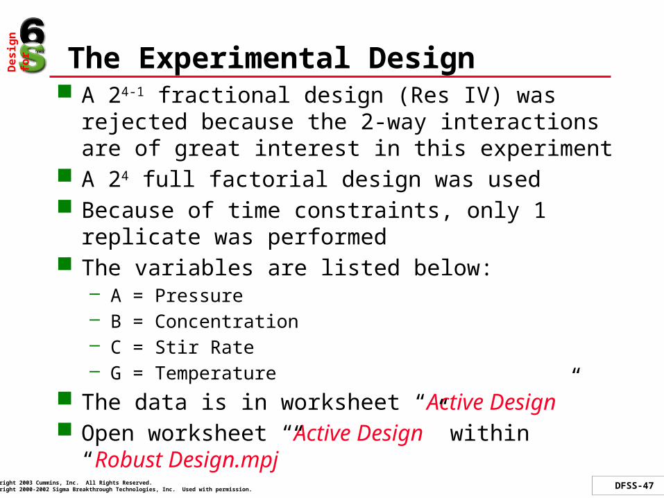
The Experimental Design A 24-1 fractional design (Res IV) was rejected because
the 2-way interactions are of great interest in this experiment
A 24 full factorial design was used Because of time constraints, only 1 replicate was
performed The variables are listed below:
– A = Pressure– B = Concentration– C = Stir Rate– G = Temperature
The data is in worksheet “Active Design” Open worksheet “Active Design” within “Robust
Design.mpj”

Factorial Analysis
This DOE is an unreplicated, 4-factor full factorial– We need to create the “Pareto of Effects” chart
Stat > DOE > Factorial > Analyze Factorial Design
Term
Effect
AC
ACD
BCD
ABCD
AB
BC
ABC
AD
ABD
A
B
C
CD
BD
D
20151050
0.08Factor
G
NameA AB BC CD
Pareto Chart of the Effects(response is Y4, Alpha = .20)
Lenth's PSE = 0.05625

Fit the Reduced Model
Stat > DOE > Factorial > Analyze Factorial Design
Based on the p-values, the A*G and B*G and C*G interactions are important. Since we have identified some important control*noise interactions, the next step is to examine the interaction plots.
Estimated Effects and Coefficients for Y4 (coded units)
Term Effect Coef SE Coef T PConstant 70.081 0.006250 11213.00 0.000A 5.987 2.994 0.006250 479.00 0.000B 9.787 4.894 0.006250 783.00 0.000C 14.612 7.306 0.006250 1169.00 0.000G 21.387 10.694 0.006250 1711.00 0.000A*B -0.038 -0.019 0.006250 -3.00 0.058A*G -0.087 -0.044 0.006250 -7.00 0.006B*C -0.062 -0.031 0.006250 -5.00 0.015B*G -18.038 -9.019 0.006250 -1443.00 0.000C*G 16.638 8.319 0.006250 1331.00 0.000A*B*C 0.062 0.031 0.006250 5.00 0.015A*B*G 0.137 0.069 0.006250 11.00 0.002A*B*C*G 0.037 0.019 0.006250 3.00 0.058

Interaction Plot
The interaction plot show the valuable interactions available to the designer. Let’s take a closer look at the strongest ones.
Stat > DOE > Factorial > Factorial Plots > Interaction Plot
A
C
G
B
51 200150 1-1
100
75
50100
75
50100
75
50
A1020
B15
C150200
Interaction Plot (data means) for Y4

Interaction Plot – A Closer Look
G
Mean
1-1
100
80
60
40
B15
G
Mean
1-1
100
80
60
40
C150200
Interaction Plot (data means) for Y4
The two interaction plots at right indicate that both B and C can be exploited to desensitize Y4 to the noise variable G– If B is set at its high level, the
slope of the G effect line is minimized
– If C is set at its low level, the slope of the G effect line is also minimized
To minimize output variation due to noise in ambient temperature (G), the above two settings should be controlled in the design

Main Effects Plot
Since factor A is not involved in a significant interaction and its main effect is significant, we should take a look at its main effect plot to see if there is some potential value in controlling A
This plot indicates that factor A has about +/- 3 units of control over the nominal value of Y4. Thus, if manipulating one of the other factors takes the mean value off target, this factor could be used to exert some control over the mean value of Y.
Stat > DOE > Factorial > Factorial Plots > Main Effects Plot
A
Mean o
f Y4
2010
73
72
71
70
69
68
67
Main Effects Plot (data means) for Y4

New Settings : Capability Analysis
B was set to 5, C was set to 150, A was left at nominal (15) It appears that the changes to B & C were successful in reducing
variation in Y4 but the mean is now off target Use factor A to adjust back to target!
78757269666360
LSL USLProcess Data
Sample N 100StDev(Within) 2.06587StDev(Overall) 2.15042
LSL 60Target *USL 80Sample Mean 67.898
Potential (Within) Capability
Overall Capability
Pp 1.55PPL 1.22PPU 1.88Ppk 1.22Cpm
Cp
*
1.61CPL 1.27CPU 1.95Cpk 1.27
Observed PerformancePPM < LSL 0.00PPM > USL 0.00PPM Total 0.00
Exp. Within PerformancePPM < LSL 65.90PPM > USL 0.00PPM Total 65.90
Exp. Overall PerformancePPM < LSL 119.97PPM > USL 0.01PPM Total 119.98
WithinOverall
Process Capability of Y4Valid

How much should we shift factor A?
Set up the response optimizer to target 70. The lower and upper limits are not important since we will manually manipulate this.
Set factor B=5 and factor C=150. The optimizer indicates a nominal Y4=67.7, very close to that observed in the validation study.
Finally, slowly slide the bar for factor A to the right while observing the predicted value of Y4. This indicates that a nominal setting of A=18.8 should achieve Y4=70.
Hi
Lo0.99934D
New
Cur
d = 0.99934
Targ: 70.0Y4
y = 69.9987
-1.0
1.0
150.0
200.0
1.0
5.0
10.0
20.0B C GA
[18.80] [5.0] [150.0] [-0.0076]
Worksheet “active design”
Stat > DOE > Factorial > Response Optimizer
Hi
Lo0.00000D
New
Cur
d = 0.00000
Targ: 70.0Y4
y = 67.7506
-1.0
1.0
150.0
200.0
1.0
5.0
10.0
20.0B C GA
[15.0] [5.0] [150.0] [-0.0076]
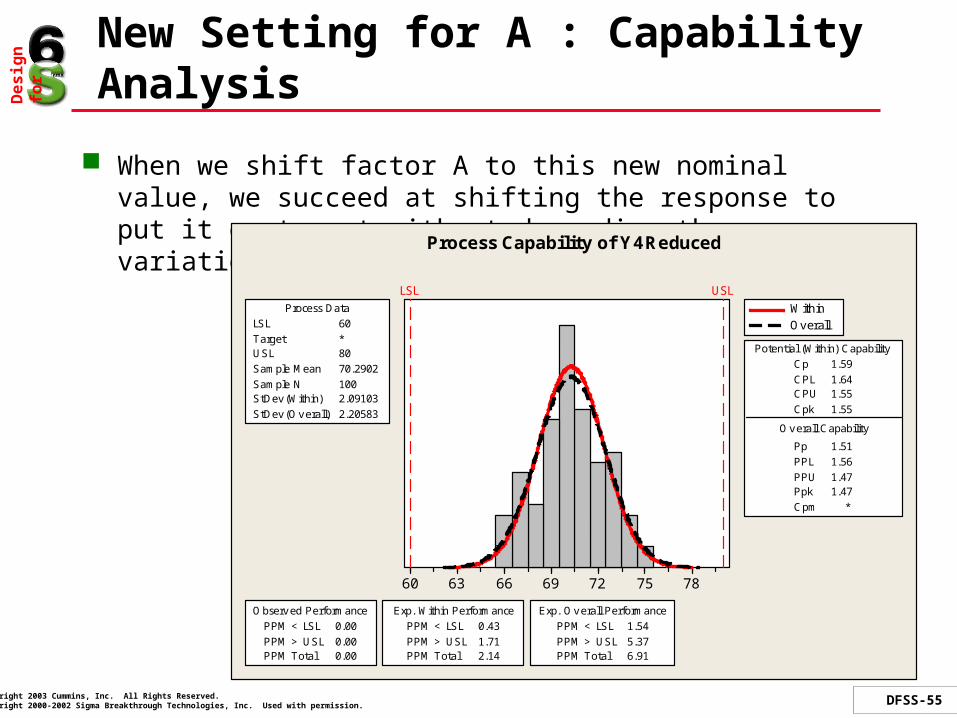
New Setting for A : Capability Analysis
When we shift factor A to this new nominal value, we succeed at shifting the response to put it on target without degrading the variation
78757269666360
LSL USLProcess Data
Sample N 100StDev(Within) 2.09103StDev(Overall) 2.20583
LSL 60Target *USL 80Sample Mean 70.2902
Potential (Within) Capability
Overall Capability
Pp 1.51PPL 1.56PPU 1.47Ppk 1.47Cpm
Cp
*
1.59CPL 1.64CPU 1.55Cpk 1.55
Observed PerformancePPM < LSL 0.00PPM > USL 0.00PPM Total 0.00
Exp. Within PerformancePPM < LSL 0.43PPM > USL 1.71PPM Total 2.14
Exp. Overall PerformancePPM < LSL 1.54PPM > USL 5.37PPM Total 6.91
WithinOverall
Process Capability of Y4Reduced
Summary
Variation improvement strategies can take two forms:– Passive Approach– Active Approach
The choice of which strategy to use depends on the ability to control or manipulate noise factors (at least for the duration of the experiment)
Standard full and fractional designs can be used Variation effects must be calculated using replications A log transform of the variability response is automatically used
to minimize the effects of asymmetry in the variance distribution The response optimizer can be used to simultaneously optimize
both mean and variability responses A validation study must be made at the end of a Robust
Parameter Design study
Desig
n
for
DFSS-57Copyright 2003 Cummins, Inc. All Rights Reserved.Copyright 2000-2002 Sigma Breakthrough Technologies, Inc. Used with permission.
Objectives Revisited
At the end of this module, participants should be able to :
Identify possible variation effects from residual plots Create a variability response from replicates Identify possible mean and variance adjustment
factors from noise-factor interaction plots Use the MINITAB Response Optimizer to achieve a
process on target with minimum variation Complete validation capability studies
Recommended