Hydrology 2019; 7(2): 32-37
http://www.sciencepublishinggroup.com/j/hyd
doi: 10.11648/j.hyd.20190702.12
ISSN: 2330-7609 (Print); ISSN: 2330-7617 (Online)
Experimental Study of the Dominant Flow Paths and Analysis of the Influence Factors Through Fracture Networks
Mu Wang1, 2, *, Fengjun Gao2, Jiazhong Qian2
1Anhui Guozhen Environmental Restoration Company Limited by Shares, Hefei, China 2School of Resources and Environmental Engineering, Hefei University of Technology, Hefei, China
Email address:
*Corresponding author
To cite this article: Mu Wang, Fengjun Gao, Jiazhong Qian. Experimental Study of the Dominant Flow Paths and Analysis of the Influence Factors Through
Fracture Networks. Hydrology. Vol. 7, No. 2, 2019, pp. 32-37. doi: 10.11648/j.hyd.20190702.12
Received: July 11, 2019; Accepted: August 12, 2019; Published: August 26, 2019
Abstract: As the main carrier of groundwater in nature, water transport behavior in fracture networks and identification of its
main control factors are challenging problems in hydrogeology. Laboratory experiments are designed in this paper using fracture
networks made of Perspex plate for a series of hydraulic tests. Using the conditions of different types of connections for inlet and
outlet, temperature tracing tests are conducted for determining dominant flow paths. The flow resistances are calculated at
different points, and the control factors of the dominant flow paths are then discussed. Three major conclusions are obtained: (1)
the existence of the dominant flow phenomenon in fracture networks is verified; (2) the dominant flow paths can be ascertained
by monitoring the temperature variation of hot water in complex fracture networks; (3) the flow resistance is the most
fundamental reason for forming dominant flow: the channel with less resistance is selected as the dominant path.
Keywords: Dominant Flow Paths, Temperature Tracer, Flow Resistance, Fracture Networks
1. Introduction
Fracture formations are ubiquitous in nature and are related
to a number of geological activities including the exploitation of
shale gas. Fracture formations may occur in the form of a single
fracture or in a fracture network, in which the fracture network
is the common ingredient, making the study of water flow in
fracture networks an attractive topic. Cherubini et al. [1]
investigated non-linear flow by analyzing hydraulic tests on an
artificially-created fractured rock sample, and the result showed
that the relationship between the flow rate discharge and the
head gradient characterized a strong inertial regime. Zhang et al.
[2] investigated the fluid flow regimes through deformable rock
fractures by conducting water flow tests through both mated
and non-mated sandstone fractures. Quinn et al. [3] quantified
the non-Darcian flow by packer testing. They found that the
flow is non-linear but not quadratic in nature. Chen et al. [4]
conducted test and simulation for the fracture network
dominant flow, the results showing that under the same
hydraulic conditions, water flowing through a fracture network
made an earlier transition to a turbulent state than through a
single fracture, by the effect of fracture intersection.
Determination of flow paths is the foundational research of
fracture networks: the dominant flow is formed where the flow
is concentrated. Berkowitz [5] summarized the flow and solute
transport laws of heterogeneous fractured rock mass, and
pointed out that the dominant flow path in fracture networks
was the most important factor affecting fracture flow. Salve [6]
conducted field tests to study the dominant flow and formation
mechanisms in different rock fractures. The study shown that
the number of fracture seepage channels in the rock mass only
accounted for 10% to 20% of the total, the remaining fractures
were mostly disconnected or poorly conductive. Figueiredo et
al. [7] carried out both laboratory and field tests, since the
experimental results of water flow and solute transport in the
conventional sealed fracture network model may be inaccurate
when compared to the actual situation. In the sparse channel,
penetration was dominated by the shape of the fracture, and the
size and direction of the fracture had less impact. Domestic
scholar, Tian [8] found the phenomenon of fracture water bias
33 Mu Wang et al.: Experimental Study of the Dominant Flow Paths and Analysis of the Influence
Factors Through Fracture Networks
flow by studying unequal cross fractures and explained the
formation mechanism of fracture water runoff. Yang et al. [9]
designed the physical model of cross-fracture with different
aspects of ratio and roughness, and simulated the experimental
data by using Fluent software, and studied the non-Darcy bias
effect characteristics of the cross-rough fracture under the
condition of high flow rate.
However, it is difficult to recognize dominant flow paths
given the complexity and high numbers of channels. Seepage
characteristics have been the subject of several studies
monitoring temperature data in fracture media. Rau et al. [10]
proposed that temperature could be used to monitor
groundwater seepage exchange. Temperature was widely used
as a tracer in the study of groundwater after the development
of the waterproof temperature recorder. Becker [11] used
airborne temperature sensors to study regional groundwater
flow. Silliman and Robinson [12] estimated the position of
fracture with the change of temperature, the contamination of
limestone fracture aquifer from surface sewage infiltration
was studied by using a temperature tracer. Klepikova et al. [13]
compared the different test methods based on the principle of
dominant flow, and proposed that temperature tomography
seemed to be an effective method to detect the dominant flow
path and characterize its hydraulic properties. Cherubini et al.
[14] designed experimental tests on heat transport in the
fracture network, and simulated temperature curves with a
particular network model, the results showing that heat
transport appeared to delay the effect compared with solute
transport. In this study, temperature data is calculated as a
tracer for reflecting the dominant flow paths.
Many scholars have used different methods to analyze
numerous control factors for forming the dominant flow paths,
such as fracture connectivity, geometric characteristics and
degree of filling. Tian [15] proposed three important hydraulic
characteristics for the theory of fracture water bias flow. One
was bias flow, another, deflection, and the third was the law of
resistance inequality, all significant reasons for the formation
of dominant flow in fractured media. Gong and Rossen [16]
focused on the influence of fracture aperture distribution, and
found that even a well-connected fracture network could
behave like a much sparser network when the aperture
distribution was broad enough. Chuang et al. [17] used
nanoscale zero-valent iron (nZVI) particles as tracers to
characterize fracture connectivity between two boreholes in
fractured rock. The position where the maximum weight of
attracted nZVI particles was observed coincides with the
depth of a permeable fracture zone delineated by the
heat-pulse flowmeter. Somogyvári et al. [18] presented a
novel concept by using a transdimensional inversion method
to invert a two-dimensional cross-well discrete fracture
network (DFN) geometry from tracer tomography
experiments. The procedure successfully identified major
transport pathways in the investigated domain and explored
equally probable DFN realizations, which were analyzed in
fracture probability maps and by multidimensional scaling.
To sum up, there are few articles about analyzing the
influence of flow resistance to dominant flow paths through
fracture networks. Therefore, this issue is discussed by
method of laboratory experiments. The purposes of this study
are to: (1) verify the existence of dominant flow phenomenon
in fracture networks; (2) ascertain the dominant flow paths of
different fracture connection types; and (3) analyze the
influence factors to dominant flow paths.
2. Basic Equations
From the perspective of fluid mechanics, the reason for the
dominant flow in the fracture networks is that the water flows
in different channels affected by different resistances. The
large flux, the less resistance. In the calculation process of
project, the energy loss is divided into two categories
according to whether the side wall of the fluid contact changes
along the path: energy loss along the path and local energy
loss. When the boundary of the channel is nearly unchanged
along the path, the flow resistance is also unchanged basically,
which is called the frictional resistance. The head loss caused
by the frictional resistance can be expressed as:
hf = λl
2b
v2
2g (1)
where l is the fracture length, b is the aperture, v is the average
velocity, and � is the resistance coefficient, it can be
calculated by:
λ = 0.11 �68
Re�
0.25
(2)
where Re is the Reynolds number of corresponding velocity, it
is expressed as:
Re = vb
υ (3)
where υ is the kinematic viscosity of the fluid (in this experiment,
the value of kinematic viscosity is 1.2028×10⁻⁶ m2/s).
When the fluid flows through various local obstacles, the
uniform flow is destroyed in this local area due to the change
of flux or boundary, causing the change of the distribution,
size or direction of the flow velocity. This resistance brings
energy loss in the pipeline and is called local resistance. The
head loss caused by the local resistance can be expressed as:
hm = ξv2
2g (4)
where � is the local resistance coefficient, the corresponding
values of � under conditions of different cross angles can be
found in the common data of the water supply and drainage
design manual, as shown in Table 1.
Table 1. Statistics of local resistance coefficient of cross fracture.
cross angle 0 10 20 30 40 50 60 70 75 80 85
� 0.50 0.56 0.63 0.70 0.78 0.85 0.91 0.96 0.98 0.99 1.00
Hydrology 2019; 7(2): 32-37 34
In the fracture networks, the water flow resistance needs to
consider both the frictional resistance and the local resistance,
then the head loss of each channel is expressed as:
h =��+� (5)
3. Experimental Design
3.1. Experimental Setup
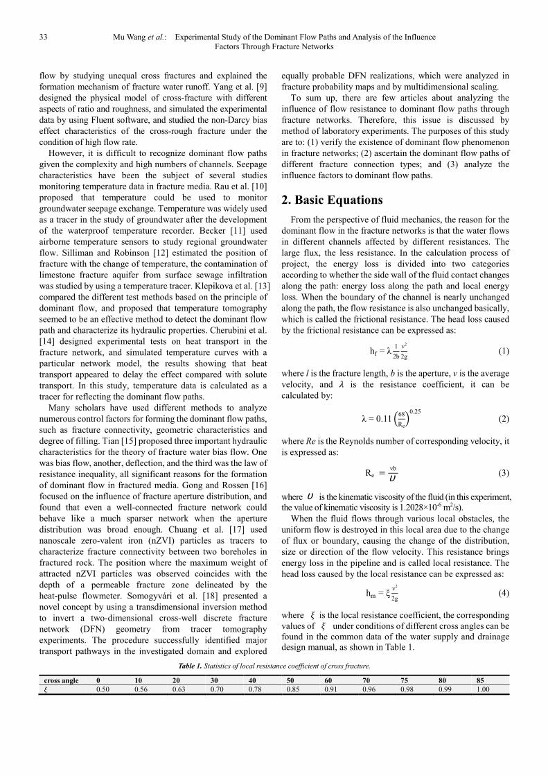
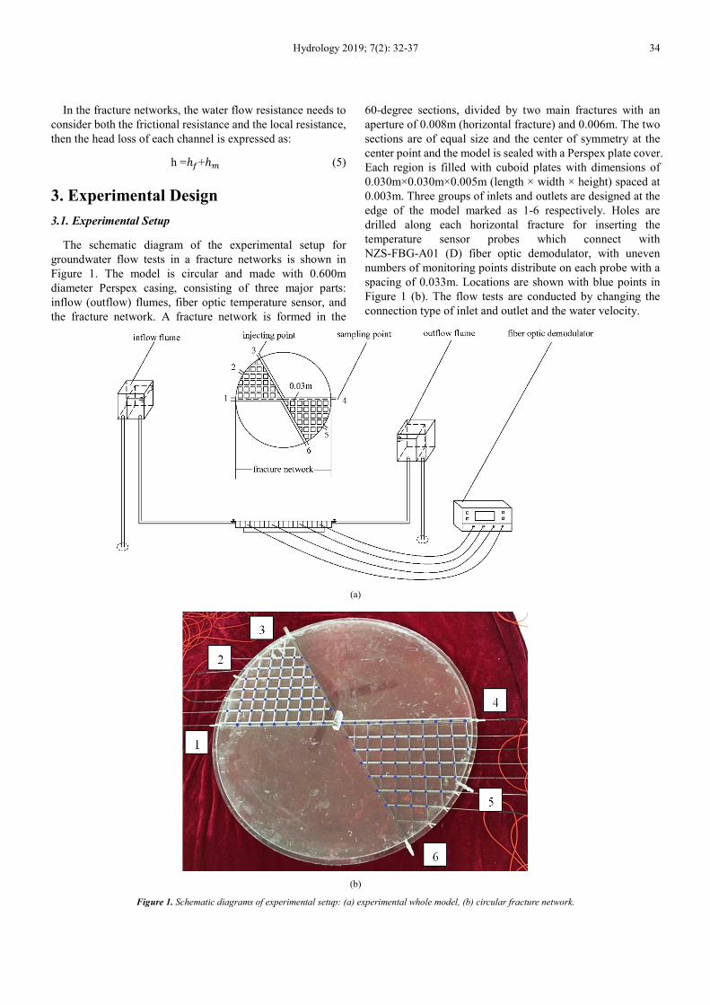
The schematic diagram of the experimental setup for
groundwater flow tests in a fracture networks is shown in
Figure 1. The model is circular and made with 0.600m
diameter Perspex casing, consisting of three major parts:
inflow (outflow) flumes, fiber optic temperature sensor, and
the fracture network. A fracture network is formed in the
60-degree sections, divided by two main fractures with an
aperture of 0.008m (horizontal fracture) and 0.006m. The two
sections are of equal size and the center of symmetry at the
center point and the model is sealed with a Perspex plate cover.
Each region is filled with cuboid plates with dimensions of
0.030m×0.030m×0.005m (length × width × height) spaced at
0.003m. Three groups of inlets and outlets are designed at the
edge of the model marked as 1-6 respectively. Holes are
drilled along each horizontal fracture for inserting the
temperature sensor probes which connect with
NZS-FBG-A01 (D) fiber optic demodulator, with uneven
numbers of monitoring points distribute on each probe with a
spacing of 0.033m. Locations are shown with blue points in
Figure 1 (b). The flow tests are conducted by changing the
connection type of inlet and outlet and the water velocity.
(a)
(b)
Figure 1. Schematic diagrams of experimental setup: (a) experimental whole model, (b) circular fracture network.

35 Mu Wang et al.: Experimental Study of the Dominant Flow Paths and Analysis of the Influence
Factors Through Fracture Networks
3.2. Testing Method
The cylinder is used to measure the steady flow rate, with an
error rate less than 2%. The water level is measured by
piezometric tubes with an error of ±0.0005m. The value of
temperature variation is equal to the temperature coefficient
multiplied by the value of the wavelength variation, which is
monitored by the probe with an error of ±0.1 degree.
4. Experimental Results and Discussions
There are four connection types in the circular fracture
network: inlet 2-outlet 5, inlet 2-outlet 6, inlet 3-outlet 5, and
inlet 3-outlet 6. The original experimental data includes the
water head, flux and temperature data (calculate from
wavelength values) in the fracture network.
4.1. Verification the Existence of Dominant Flow
Phenomenon
(a)
(b)
Figure 2. Schematic diagram of dominant flow path of inlet 3-outlet 6 in
circular fracture networks: (a) brilliant blue transport path, (b) diagram of
temperature variation.
During every test, 10 mL of hot water is injected into the
channels, the wavelengths of water are monitored under the
condition of different velocities then the temperature values
of different monitoring points are calculated. For example,
under the condition of inlet 3-outlet 6, hot water is injected
with brilliant blue. The initial transport path of brilliant
blue is shown in Figure 2 (a), where the main fracture of
inlet 3-outlet 6 is the dominant flow path obviously. It is
found that the value of the temperature variation at the
monitoring points in this main fracture is at its maximum in
each probe.
From here, the boundary condition of the circular fracture
networks is constructed according to the values of temperature
variation monitored by each probe point. The interpolation
algorithm is used in Surfer® to generate grid files for obtaining
the temperature distribution diagram covering the entire
model area. Different colors are used to indicate the
temperature levels, and the dominant flow path is structured
by connecting the maximum values, the result is shown in
Figure 2 (b). The existence of the dominant flow phenomenon
in the network crack is thus confirmed, and it is reasonable to
connect the monitoring points with the maximum values of
temperature variation for forming the dominant flow paths.
4.2. Ascertaining the Dominant Flow Paths of Fracture
Network
In order to display the dominant flow paths more clearly,
three-dimensional histograms are drawn using Python
software based on the temperature monitoring data. The
column heights and different colors are used to reflect the
temperature variation of each probe, and dominant flow
paths are constituted by connecting them. Taking the flow
rate of 0.002m/s and the hot water injection amount of 20 mL
as an example, the monitoring of temperature distribution
obtained at 24s and the corresponding dominant flow paths
are shown in Figure 3.
In Figure 3 (a), hot water is injected into inlet 2, the peak
points of temperature variation distribute along network
channels into the main fracture with aperture of 0.008m, then
circuitously leads to outlet 5. In Figure 3 (c), the distribution
of the peak points is initially similar to Figure 3 (a), but then
directly to outlet 6. In Figure 3 (e) and 3 (g), hot water is
injected into inlet 3, the peak points distribute in the main
fracture with an aperture of 0.006m, then meander to outlet 5
and directly leads to outlet 6, respectively. The Figure 3 (b),
(d), (f), (h) are the dominant flow paths drawn according to
the figures of temperature variation on the left side,
respectively.

Hydrology 2019; 7(2): 32-37 36
Figure 3. Temperature variation and dominant flow paths in circular fracture networks: (a) and (b) inlet 2-outlet 5, (c) and (d) inlet 2-outlet 6, (e) and (f) inlet
3-outlet 5, (g) and (h) inlet 3-outlet 6.
4.3. Analysis the Influence Factors to Dominant Flow Paths
From the analysis above, water flow in different channels is
affected by different resistances in the fracture networks.
There is little resistance with a fast flow rate, and this forms
the dominant flow paths. Taking inlet 2-outlet 5 as an example,
the first influence factor of direction from inlet to outlet is
marked, and the corresponding head losses of possible
channels are expressed as h1 and h2, they are shown in Figure 4.
The specific path is controlled by the flow resistance, this is
the second and most important influence factor. The third
influence factor is the main fracture with aperture of 0.008m
for the increasing of aperture. The values of h1 and h2 are
calculated by equation 5 under the condition of different flow
velocities, the results are shown in Table 2.
Figure 4. Diagram analysis the influence factors to dominant flow paths.

37 Mu Wang et al.: Experimental Study of the Dominant Flow Paths and Analysis of the Influence
Factors Through Fracture Networks
Table 2. Statistics of flow resistance of different channels in circular fracture
networks.
Flow velocities (m/s, ˟10-3) Values of h1 (m, ˟10-3) Values of h2 (m, ˟10-3)
0.95 1.50 10.07
1.28 2.12 13.48
1.64 2.52 17.62
1.77 3.03 20.14
1.95 3.54 23.15
2.24 4.62 27.66
2.46 5.37 31.72
2.77 6.56 40.33
3.15 7.64 50.26
The values of h1 are all smaller than that of h2 in Table 2, it
means the flow resistance of horizontal channel is less than the
vertical channel, and their difference increases with the
increase of flow velocity, the channel with less resistance is
selected by water, and then dominant flow paths of horizontal
direction are formed in Figure 4. On the vertical direction,
flow are influenced by the main fracture with aperture of
0.008m more than other factors, about how to quantitatively
analyze this attraction, further study is needed.
5. Conclusions
A model of fracture networks including of different inlets
and outlets is designed in this paper, a series of hydraulic tests
and temperature tracing tests are conducted under different
conditions. From the analysis above, the following
conclusions are drawn:
Firstly, water doesn’t flow uniformly in the fracture
networks, the phenomenon of dominant flow is existed and it
can be verified through brilliant blue tracing tests. Secondly, it
is difficult to monitor the values of flow velocities
continuously in the channels of fracture networks, then the
dominant flow paths can be determined by monitoring the
values of temperature variation because water flow is a carrier
of temperature. Lastly, the dominant flow paths are influenced
by many factors including the flow direction from inlet to
outlet, the flow resistance, and the aperture variation of
fracture channels. The flow resistance is the most fundamental
reason among them, flow finally chooses the channel with the
least resistance under the action of various factors.
Acknowledgements
This work was supported by the National Natural Science
Foundation of China: Experiment and Simulation of
Groundwater Selective Flow in Fracture networks (Grant No.
41772250).
References
[1] Cherubini C., Giasi C. I., and Pastore N. Bench scale laboratory tests to analyze non-linear flow in fractured media [J]. Hydrology and Earth System Sciences, 2012, 16 (8): 2511-2522.
[2] Zhang Z., Nemcik J. Fluid flow regimes and nonlinear flow
characteristics in deformable rock fractures [J]. Journal of Hydrology, 2013, 477: 139-151.
[3] Quinn P. M., Cherry J. A., and Parker B. L. Quantification of non-Darcian flow Observed during packer testing in fractured sedimentary rock [J]. Water Resources Research, 2011, 47 (9): W09533.
[4] Chen X. B., Zhao J., and Chen L. Experimental and Numerical Investigation of Preferential Flow in Fractured Network with Clogging Process [J]. Mathematical Problems in Engineering, 2014, 2014 (3): 1-13.
[5] Berkowitz B. Characterizing flow and transport in fractured geological media: A review [J]. Advances in Water Resources, 2002, 25 (8): 861-884.
[6] Salve R. Observations of preferential flow during a liquid release experiment in fractured welded tuffs [J]. Water Resources Research, 2005, 41 (9): 477-487.
[7] Figueiredo B., Tsang C. F., Niemi A., et al. Review: The state-of-art of sparse channel models and their applicability to performance assessment of radioactive waste repositories in fractured crystalline formations [J]. Hydrogeology Journal, 2016, 24 (7): 1-16.
[8] Tian K. M. Bias flow and vein fracture water runoff [J]. Geological Review, 1983, 29 (5): 408-417.
[9] Yang H. H., Wang Y., Gao W., Niu Y. L. Effect of wide-gap ratio and roughness on high-speed non-Darcy bias flow effect of cross-fracture [J]. Science Technology and Engineering, 2018, 18 (7): 44-49.
[10] Rau G. C., Andersen M. S., Mccallum A. M., et al. Analytical methods that use natural heat as a tracer to quantify surface water-groundwater exchange, evaluated using field temperature records [J]. Hydrogeology Journal, 2010, 18 (5): 1093-1110.
[11] Becker M. W. Potential for Satellite Remote Sensing of Ground Water [J]. Groundwater, 2006, 44 (2): 306–318.
[12] Silliman S., Robinson R. Identifying fracture interconnections between boreholes using natural temperature profiling: I. Conceptual Basis [J]. Groundwater, 1989, 27 (3): 393–402.
[13] Klepikova M. V., Borgne T. L., Bour O., et al. Passive temperature tomography experiments to characterize transmissivity and connectivity of preferential flow paths in fractured media [J]. Journal of Hydrology, 2014, 512 (9): 549-562.
[14] Cherubini C., Pastore N., Giasi C. I., et al. Laboratory experimental investigation of heat transport in fractured media [J]. Nonlinear Processes in Geophysics, 2017, 24 (1): 1-37.
[15] Tian K. M.. The hydraulic properties of crossing-flow in an intersected fracture [J]. Acta Geological Sinica, 1986 (2): 90-102.
[16] Gong J., Rossen W. R. Modeling flow in naturally fractured reservoirs: effect of fracture aperture distribution on dominant sub-network for flow [J]. Petroleum Science, 2017, 14 (1): 138-154.
[17] Chuang P. Y., Chia Y., Chiu Y. C., et al. Mapping fracture flow paths with a nanoscale zero-valent iron tracer test and a flowmeter test [J]. Hydrogeology Journal, 2017, 26 (1): 321-331.
[18] Somogyvári M., Jalali M., Jimenez P. S., et al. Synthetic fracture networks characterization with transdimensional inversion [J]. Water Resources Research, 2017, 53 (6): 5104-5123.
Recommended