METHODS AND RESOURCES
Extent and context dependence of pleiotropy
revealed by high-throughput single-cell
phenotyping
Kerry A. Geiler-SamerotteID1,2*, Shuang LiID
1,3, Charalampos LazarisID1,4, Austin Taylor1,
Naomi ZivID1,5, Chelsea Ramjeawan1, Annalise B. PaabyID
6, Mark L. SiegalID1
1 Center for Genomics and Systems Biology, Department of Biology, New York University, New York,
New York, United States of America, 2 Center for Mechanisms of Evolution, Biodesign Institutes, School of
Life Sciences, Arizona State University, Tempe, Arizona, United States of America, 3 Department of
Pharmacology, University of North Carolina at Chapel Hill, Chapel Hill, North Carolina, United States of
America, 4 Whitehead Institute for Biomedical Research, Cambridge, Massachusetts, United States of
America, 5 Department of Microbiology and Immunology, University of California, San Francisco, California,
United States of America, 6 School of Biological Sciences, Georgia Institute of Technology, Atlanta, Georgia,
United States of America
Abstract
Pleiotropy—when a single mutation affects multiple traits—is a controversial topic with far-
reaching implications. Pleiotropy plays a central role in debates about how complex traits
evolve and whether biological systems are modular or are organized such that every gene
has the potential to affect many traits. Pleiotropy is also critical to initiatives in evolutionary
medicine that seek to trap infectious microbes or tumors by selecting for mutations that
encourage growth in some conditions at the expense of others. Research in these fields,
and others, would benefit from understanding the extent to which pleiotropy reflects inherent
relationships among phenotypes that correlate no matter the perturbation (vertical pleio-
tropy). Alternatively, pleiotropy may result from genetic changes that impose correlations
between otherwise independent traits (horizontal pleiotropy). We distinguish these possibili-
ties by using clonal populations of yeast cells to quantify the inherent relationships between
single-cell morphological features. Then, we demonstrate how often these relationships
underlie vertical pleiotropy and how often these relationships are modified by genetic vari-
ants (quantitative trait loci [QTL]) acting via horizontal pleiotropy. Our comprehensive screen
measures thousands of pairwise trait correlations across hundreds of thousands of yeast
cells and reveals ample evidence of both vertical and horizontal pleiotropy. Additionally, we
observe that the correlations between traits can change with the environment, genetic back-
ground, and cell-cycle position. These changing dependencies suggest a nuanced view of
pleiotropy: biological systems demonstrate limited pleiotropy in any given context, but
across contexts (e.g., across diverse environments and genetic backgrounds) each genetic
change has the potential to influence a larger number of traits. Our method suggests that
exploiting pleiotropy for applications in evolutionary medicine would benefit from focusing on
traits with correlations that are less dependent on context.
PLOS BIOLOGY
PLOS Biology | https://doi.org/10.1371/journal.pbio.3000836 August 17, 2020 1 / 32
a1111111111
a1111111111
a1111111111
a1111111111
a1111111111
OPEN ACCESS
Citation: Geiler-Samerotte KA, Li S, Lazaris C,
Taylor A, Ziv N, Ramjeawan C, et al. (2020) Extent
and context dependence of pleiotropy revealed by
high-throughput single-cell phenotyping. PLoS Biol
18(8): e3000836. https://doi.org/10.1371/journal.
pbio.3000836
Academic Editor: Csaba Pal, Biological Research
Centre, HUNGARY
Received: September 24, 2019
Accepted: July 31, 2020
Published: August 17, 2020
Peer Review History: PLOS recognizes the
benefits of transparency in the peer review
process; therefore, we enable the publication of
all of the content of peer review and author
responses alongside final, published articles. The
editorial history of this article is available here:
https://doi.org/10.1371/journal.pbio.3000836
Copyright: © 2020 Geiler-Samerotte et al. This is
an open access article distributed under the terms
of the Creative Commons Attribution License,
which permits unrestricted use, distribution, and
reproduction in any medium, provided the original
author and source are credited.
Data Availability Statement: All data are available
at open science framework DOI 10.17605/OSF.IO/
B7NY5.

Introduction
Pleiotropy exists when a single mutation affects multiple traits [1,2]. Often, pleiotropy is
defined instead as a single gene contributing to multiple traits, although what is implied is the
original definition—that a single change at the genetic level can have multiple consequences at
the phenotypic level [2]. As our ability to survey the influence of genotype on phenotype
improves, examples of pleiotropy are growing [3–8]. For example, individual genetic variants
have been associated with seemingly disparate immune, neurological, and digestive symptoms
in humans and mice [9,10]. Genes affecting rates of cell division across diverse environments
and drug treatments have been identified in microbes and cancers [11,12]. A view emerging
from genome-wide association studies is that variation in complex traits is “omnigenic” in the
sense that many loci indirectly contribute to variation in many traits [13,14].
However, the extent of pleiotropy remains a major topic of debate because, despite its
apparent prevalence, pleiotropy is thought to be evolutionarily disadvantageous. The more
traits a mutation affects, the more likely it is that the mutation will have a negative impact on
at least one. Pervasive pleiotropy should therefore constrain evolution [15], exacting what is
known as a cost of complexity or cost of pleiotropy [11,16–19]. This cost may bias which muta-
tions underlie adaptation, for example, toward less-pleiotropic cis-regulatory changes over
more-pleiotropic changes in trans-acting factors [20,21], or toward changes to proteins that
participate in relatively few biological processes [22,23]. Over long periods, the cost of pleio-
tropy may influence the organization of biological systems, favoring a modular structure in
which genetic changes influencing one group of traits have minimal impact system-wide
[24–29].
At stake in the ongoing debate about the extent of pleiotropy [30–33] are some of modern
biology’s prime objectives, including the prediction of complex phenotypes from genotype
data [18,34,35] and the prediction of how organisms will adapt to environmental change
[36,37]. These predictions are more challenging if genetic changes influence a large number of
traits with complex interdependencies. Nonetheless, understanding how a given mutation
influences multiple traits could be powerful, allowing prediction of some phenotypic responses
given others [38,39]. Indeed, recent strategies in medicine called evolutionary traps aim to
exploit pleiotropy, for example, by finding genetic changes that provide resistance to one treat-
ment while promoting susceptibility to another [40–42].
The lack of consensus about the extent of pleiotropy in natural systems is, in part, due to
poorly defined expectations for how to test for it experimentally. One key issue is that defining
a phenotype is not trivial [43,44]. Consider a variant in the apolipoprotein B gene that increases
low-density lipoprotein (LDL) cholesterol levels as well as the risk of heart disease. Elevated
LDL promotes heart disease [45], so are these two phenotypes or one? Alternatively, consider a
mutation in the phenylalanine hydroxylase gene that affects nervous system function and skin
pigmentation. These dissimilar effects, both symptoms of untreated phenylketonuria (PKU),
originate from the same problem: a deficiency in converting phenylalanine to tyrosine [46]. Is
it appropriate to call mutations that have this single metabolic effect pleiotropic? Likewise,
shall one call pleiotropic a mutation that makes tomatoes both ripen uniformly and taste bad,
when the effect of the mutation is to reduce the function of a transcription factor that pro-
motes chloroplast development, which in turn necessarily affects both coloration and sugar
accumulation [47]?
The LDL, PKU, and tomato cases are examples of vertical pleiotropy, i.e., pleiotropy that
results when one phenotype influences another or both are influenced by a shared factor
[5,43]. The alternative to vertical pleiotropy is horizontal pleiotropy, in which genetic differ-
ences induce correlations between otherwise independent phenotypes. It might be tempting to
PLOS BIOLOGY Pleiotropy revealed by high-throughput single-cell phenotyping
PLOS Biology | https://doi.org/10.1371/journal.pbio.3000836 August 17, 2020 2 / 32
Funding: This work was supported by National
Institutes of Health grant R35GM118170 (to MLS),
National Institutes of Health fellowship
F32GM103166 (to KAG-S), National Institutes of
Health grant R35GM133674 (to KAG-S), a New
York University Graduate School of Arts and
Science Dean’s Dissertation Fellowship (to SL),
and National Institutes of Health grant
R35GM119744 (to ABP). The funders had no role
in study design, data collection and analysis,
decision to publish, or preparation of the
manuscript.
Competing interests: The authors have declared
that no competing interests exist.
Abbreviations: GdA, geldanamycin; GFP, green
fluorescent protein; IQR, interquartile range; LDL,
low-density lipoprotein; MA, mutation-
accumulation; PCA, principal component analysis;
PKU, phenylketonuria; QTL, quantitative trait loci.

discard vertical pleiotropy as less “genuine” [48] or less important than horizontal pleiotropy,
but that would be a mistake because vertical pleiotropy reveals important information about
the underlying biological systems that produce the phenotypes in question. Consider the value
in identifying yet-unknown factors in heart disease by finding traits that correlate with it, or in
understanding where in a system an intervention is prone to produce undesirable side effects.
Consider also that the extent and nature of vertical pleiotropy speak directly to the question of
modularity: modularity is implied if vertical pleiotropy either is rare or manifests as small
groups of correlated traits that are isolated from other such groups. If there is modularity, then
there can be horizontal pleiotropy, when particular genetic variants make links between previ-
ously unconnected modules.
The above considerations suggest that a unified analysis that distinguishes and compares
horizontal and vertical pleiotropy is needed to make sense of the organization and evolution of
biological systems. However, existing methods of distinguishing horizontal and vertical pleio-
tropy are problematic because judgments must be made about which traits are independent
from one another. Such judgments differ between researchers and over time. Indeed, the
tomato example can be viewed as a case of horizontal pleiotropy transitioning recently to verti-
cal pleiotropy as knowledge of the underlying system advanced.
In this study, we propose and apply an empirical and analytical approach to measuring
pleiotropy that relies far less on subjective notions of what constitutes an independent pheno-
type. The key principle is that the distinction between vertical and horizontal pleiotropy lies in
whether traits are correlated in the absence of genetic variation [43]. For vertical pleiotropy,
the answer is yes: because one trait influences the other or the two share an influence, nonge-
netic perturbations that alter one phenotype are expected to alter the other. For horizontal
pleiotropy, the answer is no: genetic variation causes the trait correlation. In this study, we
determined how traits correlate in the absence of genetic variation by measuring single-cell
traits in clonal populations of cells.
We used high-throughput morphometric analysis [49–53] of hundreds of thousands of sin-
gle cells of the budding yeast Saccharomyces cerevisiae to measure how dozens of cell-morphol-
ogy traits (thousands of pairs of traits) covary within clonal populations and between such
populations representing different genotypes. Within-genotype correlations report on vertical
pleiotropy, whereas between-genotype correlations report on horizontal pleiotropy to the
extent that they exceed the corresponding within-genotype correlations. For one set of geno-
types, we used 374 progeny of a cross of two natural isolates [54], which enabled not only the
estimation of vertical and horizontal pleiotropy but also the identification of quantitative trait
loci (QTL) with pleiotropic effects. For another set of genotypes, we used a collection of muta-
tion-accumulation (MA) lines, each of which contains a small number of unique spontaneous
mutations [55,56], which enabled a more direct test of the ability of mutations to alter trait
correlations.
The traits we study—morphological features of single cells—represent important fitness-
related traits [51,57,58] that contribute to processes such as cell division and tissue invasion
(e.g., cancer metastasis [59]). Cell-morphological features may correlate across cells for a vari-
ety of vertical or horizontal reasons. Vertical reasons include (1) inherent geometric con-
straints (e.g., on cell circumference and area); (2) constraints imposed by gene-regulatory
networks (e.g., if the genes influencing a group of traits are all under control of the same tran-
scription factor); and (3) constraints induced by developmental processes (e.g., as a yeast cell
divides or “buds,” many morphological features are affected). Horizontal pleiotropy might be
evident because genetic variants each affecting two or more traits (that are otherwise weakly
correlated) are segregating in the progeny of the cross between two natural isolates. Alterna-
tively, horizontal pleiotropy might be evident because a particular allele strengthens the trait
PLOS BIOLOGY Pleiotropy revealed by high-throughput single-cell phenotyping
PLOS Biology | https://doi.org/10.1371/journal.pbio.3000836 August 17, 2020 3 / 32

correlation so that genetic variation affecting one trait is more likely to affect another when
that allele is present. These alternatives can be distinguished by examining trait correlations in
two subsets of progeny strains defined by which natural isolate’s allele they possess at a QTL of
interest.
In addition to genetic variation, nongenetic variation may also alter the correlations
between traits. We rely on nongenetic heterogeneity within clonal populations to serve as per-
turbations that reveal inherent trait correlations. However, the correlations themselves might
be heterogeneous within these populations. For example, the dependencies between morpho-
logical features may change as cells divide. To control for this possibility, we performed our
trait mapping and subsequent analysis after binning cells into three stages (unbudded, small-
budded, and large-budded cells). We further examined whether trait correlations change
across the cell cycle by using a machine-learning approach to more finely bin the imaged cells
into 48 stages of division.
Collectively, the results we present here demonstrate that both types of pleiotropy, vertical
and horizontal, are prevalent for single-cell morphological traits, suggesting that biological sys-
tems occupy a middle ground between extreme modularity and extreme interconnectedness.
Perhaps more surprisingly, we find that trait correlations are often context dependent and can
be altered by mutations as well as cell-cycle state and drug treatments. The dynamic nature of
trait correlations encourages caution when attempting to quantify and interpret the extent of
pleiotropy in nature or when making predictions about correlated phenotypic responses to the
same selection pressure, as is done when crafting evolutionary traps. However, applying our
approach may suggest which trait correlations are less context dependent and therefore more
useful in setting such traps.
Results
QTLs with pleiotropic effects influence yeast single-cell morphology
To detect genes with pleiotropic effects on cell morphology, we measured 167 single-cell mor-
phological features (e.g., cell size, bud size, bud angle, distance from nucleus to bud neck; S1
Table) in 374 yeast strains that were generated in a previous study from a mating between two
wild yeast isolates [54,60]. These wild isolates, one obtained from soil near an oak tree, the
other from a wine barrel, differ by 0.006 SNPs per site [61] and have many heritable differences
in single-cell morphology [62]. For example, we find that yeast cells from the wine strain, on
average, are smaller, are rounder, and have larger nuclei during budding than yeast cells from
the oak strain (S1 Fig).
To measure their morphologies, we harvested exponentially growing cells from three repli-
cate cultures of each of these 374 recombinant strains and imaged, on average, 800 fixed,
stained cells per strain using high-throughput microscopy in a 96-well plate format (S2 Fig).
We used control strains present on each plate to correct for plate-to-plate variation and quan-
tified morphological features using CalMorph software [53], which divides cells into three cat-
egories based on their progression through the cell cycle (i.e., unbudded, small-budded, and
large-budded cells) and measures phenotypes specific to each category.
A simple way to measure pleiotropy would be to identify QTL that contribute to variation
in these phenotypes and then to count the number of phenotypes to which each QTL contrib-
utes. However, such a measure is sensitive to the statistical thresholds that are used and there-
fore risks yielding false inferences about trait modularity. Using a liberal threshold would
cause false-positive cases of pleiotropy (less apparent modularity), whereas a conservative
threshold would cause failures to detect pleiotropic QTL when they exist (more apparent mod-
ularity). Such a measure also assumes the counted traits are somehow independent except for
PLOS BIOLOGY Pleiotropy revealed by high-throughput single-cell phenotyping
PLOS Biology | https://doi.org/10.1371/journal.pbio.3000836 August 17, 2020 4 / 32

correlations induced by genetic variants. Statistically independent traits could be constructed
(and then counted) as principal components of the original traits, but the concern about too-
liberal or too-conservative QTL-detection thresholds would remain. Moreover, as we explore
extensively below, trait correlations are hierarchical (differing within and between genotypes
and conditions), making application of principal components analysis problematic. For these
reasons, we do not focus on counting the number of phenotypes influenced by a given locus.
Still, to begin to dissect vertical and horizontal pleiotropy, we must start with candidate exam-
ples of pleiotropic loci.
To detect QTL, we used 225 markers spread throughout the genome [54] and Haley-Knott
regression implemented in the R package R/qtl [63,64]. We used a standard permutation-
based method to estimate statistical significance [63–65], with permutations performed sepa-
rately for each trait such that the per-trait probability of detecting a false positive is 0.05. With
this cutoff, we identified 41 QTL that contribute to variation in 155 of the surveyed morpho-
logical features (Fig 1A). This approach does not correct for the testing of multiple traits.
When we do so using a false-discovery rate set to 5%, results do not change qualitatively.
Indeed, the majority of QTL-trait associations that are eliminated using this more-stringent
cutoff involve QTL that are detected regardless of this correction (Fig 1A; 80% of red points
are present at QTL that also possess black points). This observation suggests many of the asso-
ciations detected with the less-stringent cutoff are not spurious. We therefore present subse-
quent analyses using the QTL-trait associations based on the less-stringent cutoff, but we also
report analyses using the reduced set of associations based on the more-stringent cutoff to
establish that qualitative conclusions did not change.
Most of the QTL we detect are pleiotropic, meaning each contributes to variation in more
than one morphological feature (Fig 1A; 36/41 QTL influence multiple traits, 20/26 after cor-
recting for testing multiple traits). The median number of traits to which each QTL contributes
is 5 (5.5 after correction). This finding provides some support for the idea that biological sys-
tems demonstrate limited pleiotropy, in that the median number of traits affected per QTL is
low (5/167). This median number of traits is similar to that found in previous high-dimen-
sional QTL screens [17,31] and in analyses of gene knockouts in yeast and mouse [11]. Further
evidence that biological systems demonstrate limited pleiotropy, and thus a modular organiza-
tion, comes from previous studies of this mapping family that show these same QTL do not
contribute to variation in sporulation efficiency [60].
However, as noted above, conclusions drawn about modularity from studies that count
traits are subject to criticism: some QTL influences may be too small to detect, even with less-
stringent significance thresholds, creating the appearance of modularity even if every QTL
influences every trait to at least some small degree. Further, we detect some QTL that influence
large numbers of traits, up to 73 (68 after correction). Although such QTL mitigate, to some
extent, concerns about detection power, they highlight other potential problems: some QTL
might contain multiple genetic differences that impact different traits, and some morphologi-
cal features might be inherently correlated and therefore should not be counted as indepen-
dent traits. Next, we focus on the first of these problems by asking whether these QTL
represent single genes that contribute to phenotypic variation in many morphological features.
We return to the issue of trait independence after that.
Single genes with pleiotropic effects influence yeast single-cell morphology
When a QTL affects multiple traits, it might not mean that variation in a single gene is contrib-
uting to variation in these traits but instead that linked genes are contributing to variation in
distinct, individual traits. We partitioned genotype-phenotype associations on the same
PLOS BIOLOGY Pleiotropy revealed by high-throughput single-cell phenotyping
PLOS Biology | https://doi.org/10.1371/journal.pbio.3000836 August 17, 2020 5 / 32

chromosome into separate QTL when they were greater than 5 cM apart, except in genome
regions where many genotype-phenotype associations are present and there is no clear break
point. A distance of 5 cM corresponds on average to eight protein-coding genes in the yeast
genome. The largest QTL we detected spans 17 cM, which is roughly half the window size uti-
lized in a previous study of this same QTL-mapping family [63]. This approach reduces but
does not eliminate the possibility that QTL represent the action of linked loci.
Fig 1. Pleiotropic QTL influence yeast single-cell morphology. The vertical axes in all plots represent the 155 CalMorph morphological traits for which we detect
QTL. These traits are sorted, from top to bottom, based on the difference between the oak and wine parental strains. (A) Of 41 QTL that contribute to variation in
single-cell morphology, 36 contribute to variation in multiple features. The horizontal axis indicates the chromosomal location of each QTL (in cM). Differently
shaped points indicate separate QTL that are more than 5 cM apart on the same chromosome. The darkness of a point represents the effect size of a QTL; effect sizes
range from 1.3% (lightest points) to 17.5% (darkest points) of the difference between parents. All points (red and black) represent genotype-phenotype associations
detected using a per-trait genome-wide type I error rate of 5%. The points highlighted in black are significant after correcting for testing multiple phenotypes using a
false-discovery rate of 5%. The QTL highlighted in pink, green, purple, and orange are very pleiotropic, contributing to 57, 30, 73, or 64 morphological features,
respectively. (B) Gene-swapping experiments demonstrate that single genes contribute to multiple morphological features. The horizontal axis represents the relative
phenotypic differences between the wine and oak parents (leftmost column) or one of these strains versus a derivative strain that differs in a single gene. The relative
phenotypic differences between a pair of strains are calculated by scaling each trait to have a mean of 0 and standard deviation of 1 across all cells in both strains, and
then subtracting the average value in one strain from that in the other. To control for variation among replicate experiments, this scaling was done independently for
each replicate experiment in which both strains were imaged. Error bars represent 95% confidence intervals inferred from the replicate experiments. The two gene
replacements shown, PXL1 and HOF1, are respectively located within the QTL highlighted in green and purple in (A). When calculating the difference between
strains, we always subtracted the trait values of the strain possessing more wine genes from those of the strain possessing more oak genes, such that the effects of the
wine or oak gene replacements appear in the same direction on all plots. Data underlying this figure can be found at https://osf.io/b7ny5/. QTL, quantitative trait
loci.
https://doi.org/10.1371/journal.pbio.3000836.g001
PLOS BIOLOGY Pleiotropy revealed by high-throughput single-cell phenotyping
PLOS Biology | https://doi.org/10.1371/journal.pbio.3000836 August 17, 2020 6 / 32

For a small number of QTL with high pleiotropy (highlighted in Fig 1A), we sought to test
whether the effects on different morphological features were due to the action of a single gene.
We performed these tests by swapping the parental versions of candidate genes (i.e., we geneti-
cally modified the wine strain to carry the oak version of a given gene, and vice versa). We
used the delitto perfetto technique to perform these swaps [66], such that the only difference
between a parental genome and the swapped genome is the coding sequence of the single can-
didate gene plus up to 1 kb of flanking sequence. Candidate genes were selected based on
descriptions of the single-cell morphologies of their knockout mutants [67] and the presence
of at least one nonsynonymous amino acid difference between the wine and oak alleles [62].
When a candidate gene contributes to the morphological differences between the wine and
oak parents, we expect yeast strains that differ at only that locus to recapitulate some of the
morphological differences between the wine and oak parents. Indeed, this is what we observe
for PXL1, a candidate for the QTL on chromosome 11, and HOF1, a candidate for the QTL on
chromosome 13 (Fig 1B; compare each plot on the right to the leftmost plot; see also S2 Table).
This influence is most pervasive for HOF1; both the oak and the wine alleles have a strong
effect on the morphology of the opposite parent, and their effects recapitulate the parental dif-
ference to a large extent. The pervasive influence of HOF1 on various morphological features
is consistent with the fact that this gene’s product affects actin-cable organization and is
involved in both polar cell growth and cytokinesis [68]. The effect of PXL1 on cell morphology
is also apparent across many single-cell features, although only the oak allele has a strong effect
that recapitulates the parental difference. We evaluated RAS1, a candidate for the QTL on
chromosome 15, but initial tests indicated that it did not have a significant impact on most
morphological features (S2 Table). We also attempted to swap alleles for a candidate gene cor-
responding to the QTL on chromosome 8 but were unsuccessful.
A previous screen for QTL influencing single-cell morphology in the progeny of a genetically
distinct pair of yeast strains (a different vineyard strain and a laboratory strain) found some of
the same pleiotropic QTL that we detect in the wine and oak cross [69] (compare their Table 2
to our S1 Table). In particular, we both find a QTL in the same position on chromosome 15 that
influences many morphological features related to nucleus size, shape, and position in the cell
(Fig 1A; orange). We also both detect a QTL near base pair 100,000 on chromosome 8 that
influences cell size and shape (Fig 1A; pink). In the previous screen, the genetic basis of this
QTL was shown to be a single nucleotide change within the GPA1 gene [69].
The main conclusion from our gene-swapping experiments, which is consistent with the
previous cell-morphology QTL study [69] as well as with comprehensive surveys of how gene
deletions affect the morphology of a laboratory yeast strain [11,49], is that single genes with
pleiotropic effects on cell morphology are readily detected in budding yeast. Moreover, the
morphological traits involved were previously shown to influence fitness [51,57,58], which
raises the question: why do so many genetic analyses (including ours) detect pleiotropy [5,9–
12,14] when other work suggests that pleiotropy exacts a cost [17,18,20,21]?
Dissecting pleiotropy using clonal populations of cells
One hypothesis to explain pervasive pleiotropy may be that the phenotypes we chose to mea-
sure are not independent. Instead, many of these single-cell morphological features may be
inherently related such that perturbing one will have unavoidable consequences on another
and thus any associated limitation of adaptation will be unavoidable as well. In other words,
the hypothesis is that much of the pleiotropy we observe is vertical pleiotropy. A test of this
hypothesis is to ask whether traits that are jointly affected by the same QTL are correlated in
the absence of genetic differences. Our dataset provides a unique opportunity to perform such
PLOS BIOLOGY Pleiotropy revealed by high-throughput single-cell phenotyping
PLOS Biology | https://doi.org/10.1371/journal.pbio.3000836 August 17, 2020 7 / 32

a test because we quantified single-cell traits for, on average, 800 clonal cells per yeast strain
(S2 Fig).
We leverage the hierarchical structure and large sample size of our dataset to obtain precise
estimates of the correlations that exist within and between strains. Thereby we learn about the
underlying relationships between morphological traits, which we use to distinguish vertical
from horizontal pleiotropy. Because we are studying clonal families without a complicated pedi-
gree structure, these within- and between-strain correlations are equivalent to the so-called
environmental and genetic correlations of quantitative genetics [70]. Here, we use a simple (and
fast) method that is appropriate for two-level hierarchical data to partition the total correlation
into a pooled within-strain component (rW) and a between-strain component (rB) [71]. One
caveat of this correlation-partitioning approach is that rB is effectively the correlation between
strain means, which can bias estimates of genetic covariance [70]. This bias is most pronounced
at small sample sizes [70], so our large sample sizes allay concern. Nonetheless, for a subset of
traits, we tested whether estimates obtained from correlation partitioning are similar to those
obtained from mixed-effect linear models that specify the variance-covariance structure of the
experimental design. Environmental correlations estimated using both methods are nearly
identical (S3 Fig). Genetic correlations estimated by correlation partitioning are sometimes
slightly smaller in magnitude than those obtained by linear modeling (S3 Fig). This bias is con-
servative; it may prevent us from identifying cases in which the environmental and genetic cor-
relations significantly differ but will not tend to create such cases. Despite this reduced power,
we rely on the correlation-partitioning approach, which is substantially faster, because our goal
is to estimate environmental and genetic correlations for thousands of trait pairs.
Unlike the mapping analysis, which considered phenotypes across all three classes of cell
type (unbudded, small-budded, and large-budded), this correlation-partitioning analysis can
only be applied to pairs of phenotypes that can be measured in the same cell. Three of the 36
pleiotropic QTL exclusively affect traits from different cell types. For example, a QTL on chro-
mosome 4 affects the shape of the nucleus in unbudded cells as well as in large-budded cells.
The correlation between these traits cannot be partitioned into a within-strain component
because these traits are never measured in the same single cell. Excluding these three QTL
leaves 33 pleiotropic QTL.
The 167 single-cell morphological features we measured represent 5,645 pairs of traits (378,
1,081, and 4,186 pairs of morphological features pertaining to unbudded, small-budded, and
large-budded cells, respectively). Because some of these traits are related, these thousands of
trait pairs are not independent. This dependence prevents us from reliably counting the abso-
lute number of traits that are influenced by vertical versus horizontal pleiotropy. Still, parti-
tioning correlations into a nongenetic (rW) and a genetic (rB) component for thousands of
trait pairs enables us to (1) analyze a network describing the degree to which morphological
traits are interconnected or modular and (2) detect examples of horizontal pleiotropy if they
exist. This approach differs from that of previous studies of pleiotropy that used principal com-
ponent analysis (PCA) to understand which traits are correlated [17]. Performing PCA on the
individual-cell data is not the same as controlling for rW because PCA would ignore the strain
groupings, which can then dominate the analysis (the classic “heterogeneous subgroup” prob-
lem in correlation analysis [72]). As a consequence, PCA can miss cases of horizontal pleio-
tropy and obscure, rather than reveal, inherent trait relationships.
Inherent relationships between traits contribute to pleiotropy
We focus first on vertical pleiotropy by analyzing correlations that exist in the absence of any
genetic differences (rW). In the analyses that follow, when we refer to rW (or rB), we mean the
PLOS BIOLOGY Pleiotropy revealed by high-throughput single-cell phenotyping
PLOS Biology | https://doi.org/10.1371/journal.pbio.3000836 August 17, 2020 8 / 32
magnitude of the correlation, as the sign has no relevance for arbitrary pairs of traits. The dis-
tribution of rW across traits that are influenced by the same QTL reflects the degree to which
that QTL acts via vertical pleiotropy. The overall pattern of rW values (i.e., whether there are
isolated clusters of highly correlated traits versus a densely interconnected network of traits)
reflects the modularity of the underlying biological system. These within-strain correlations
are estimated with extremely high precision because of our large sample size of hundreds of
thousands of clonal cells (800 per each of 374 strains).
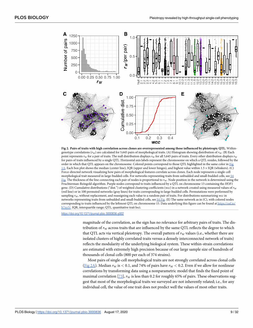
Most pairs of single-cell morphological traits are not strongly correlated across clonal cells
(Fig 2A). Median rW is< 0.1, and 74% of pairs have rW < 0.2. Even if we allow for nonlinear
correlations by transforming data using a nonparametric model that finds the fixed point of
maximal correlation [73], rW is less than 0.2 for roughly 65% of pairs. These observations sug-
gest that most of the morphological traits we surveyed are not inherently related; i.e., for any
individual cell, the value of one trait does not predict well the values of most other traits.
Fig 2. Pairs of traits with high correlation across clones are overrepresented among those influenced by pleiotropic QTL. Within-
genotype correlations (rW) are calculated for 5,645 pairs of morphological traits. (A) Histogram showing distribution of rW. (B) Each
point represents rW for a pair of traits. The null distribution displays rW for all 5,645 pairs of traits. Every other distribution displays rW
for pairs of traits influenced by a single QTL. Horizontal axis labels represent the chromosome on which a QTL resides, followed by the
order in which that QTL appears on the chromosome. Colored points correspond to those QTL highlighted in the same color in Fig
1A. Each box plot shows the median (center line), IQR (upper and lower hinges), and highest value within 1.5 × IQR (whiskers). (C)
Force-directed network visualizing how pairs of morphological features correlate across clones. Each node represents a single-cell
morphological trait measured in large-budded cells. For networks representing traits from unbudded and small-budded cells, see S4
Fig. The thickness of the line connecting each pair of nodes is proportional to rW. Node position in the network is determined using the
Fruchterman-Reingold algorithm. Purple nodes correspond to traits influenced by a QTL on chromosome 13 containing the HOF1gene. (D) Cumulative distributions (“dist.”) of weighted clustering coefficients (wcc) in a network created using measured values of rW
(red line) or in 100 permuted networks (gray lines) for traits corresponding to large-budded cells. Permutations were performed by
sampling rW, without replacement, and reassigning each value to a random pair of traits. For distributions summarizing wcc in
networks representing traits from unbudded and small-budded cells, see S4 Fig. (E) The same network as in (C), with colored nodes
corresponding to traits influenced by the leftmost QTL on chromosome 15. Data underlying this figure can be found at https://osf.io/
b7ny5/. IQR, interquartile range; QTL, quantitative trait loci.
https://doi.org/10.1371/journal.pbio.3000836.g002
PLOS BIOLOGY Pleiotropy revealed by high-throughput single-cell phenotyping
PLOS Biology | https://doi.org/10.1371/journal.pbio.3000836 August 17, 2020 9 / 32

Nonetheless, the distribution of rW has a prominent right tail (Fig 2A), indicating that some
morphological features are strongly correlated across clonal cells. These correlated features are
more likely to be influenced by pleiotropic QTL. Among pairs represented by this right tail
(specifically, those with rW > 0.2), 75% consist of traits that share at least one QTL influence;
the same is true for only 36% of pairs with rW < 0.2. These percentages are similar after chang-
ing our QTL-detection threshold to correct for having tested multiple phenotypes (66% and
21%, respectively). Further, the number of pleiotropic QTL influencing both traits in a pair
correlates with that pair’s rW (Pearson’s r is 0.52 before correction and 0.54 after). These results
suggest that inherent correlations among morphological features often cause genetic perturba-
tions to one feature to have consequences on another. In other words, we observe evidence of
vertical pleiotropy.
Next, we studied each of the 33 pleiotropic QTL one at a time, asking whether they influ-
ence pairs of traits with higher rW than expected by chance. Most QTL have a higher median
rW for the pairs of traits they influence than the median rW given by all possible pairs of traits
(Fig 2B). This difference suggests that vertical pleiotropy drives a large portion of the pleio-
tropy we detect.
We also used network analysis to move beyond the pairwise comparisons in Fig 2A and ask
if morphological traits tend to be clustered into modules. Traits with higher rW do indeed tend
to group into clusters in networks in which the single-cell morphological traits are nodes and
the rW magnitudes are edge weights (Fig 2C). This need not have been the case; pairs of traits
with high rW could have been distributed throughout the network without necessarily being
clustered near other high-rW pairs. Instead, networks representing single-cell morphological
features demonstrate more clustering than do random networks drawn from the same values
of rW (Fig 2D; for corresponding figures from unbudded and small-budded trait networks, see
S4 Fig). This observation might indicate that morphological phenotypes have a modular orga-
nization, whereby phenotypes within a module exert influence on one another but exert less
influence on phenotypes from other modules. However, this observation could also result
from human bias when enumerating phenotypes that can be measured, in the sense that phe-
notypes that bridge modules might somehow be absent from the dataset. The comprehensive
nature of CalMorph diminishes this concern. A related concern is that apparent modules are
formed by trivially related phenotypes, such as the radius and diameter of a circular object, but
we do not find such trivial relationships among the CalMorph phenotypes. Even a high corre-
lation between the length and area of the nucleus implies a constraint on nuclear aspect ratio.
Our analysis of within-strain trait correlations so far suggests that natural variation contrib-
uting to variation in multiple single-cell morphological features often acts via vertical pleio-
tropy. Still, there are hints of another mechanism at play. Some QTL tend to influence traits
that are not clustered in the correlation network (e.g., Fig 2E). And many pleiotropic QTL
influence some pairs of traits with negligible rW (Fig 2B). To investigate how often pleiotropy
is not predicted by the degree to which morphological features correlate in the absence of
genetic variation, in the next section we compare trait correlations present across clones (rW)
to those present between genetically diverse strains (rB).
Many traits are more strongly correlated across strains than they are across
clones
When genetic changes that perturb one trait have collateral effects on another, we expect the
way traits correlate across genetically diverse strains to reflect trait correlations across clones
(i.e., rB = rW). When this condition is met, pleiotropy can be viewed as an expected conse-
quence of inherent relationships between traits, i.e., vertical pleiotropy. On the other hand, if a
PLOS BIOLOGY Pleiotropy revealed by high-throughput single-cell phenotyping
PLOS Biology | https://doi.org/10.1371/journal.pbio.3000836 August 17, 2020 10 / 32
QTL influences two traits that do not correlate across clones, it may cause these traits to corre-
late across strains in which this QTL is segregating. In this case, we expect rB will be greater
than rW, suggesting horizontal pleiotropy.
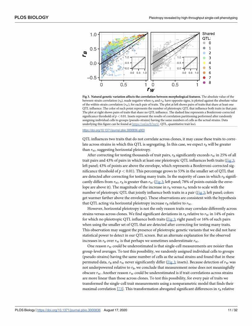
After correcting for testing thousands of trait pairs, rB significantly exceeds rW in 25% of all
trait pairs and 43% of pairs in which at least one pleiotropic QTL influences both traits (Fig 3;
left panel; 43% of points are above the envelope, which represents a Bonferroni-corrected sig-
nificance threshold of p< 0.01). This percentage grows to 53% in the smaller set of QTL that
are detected after correcting for testing many traits. In the majority of cases in which rB signifi-
cantly differs from rW, rB is greater than rW (Fig 3; left panel; 78% of points outside the enve-
lope are above it). The magnitude of the increase in rB versus rW tends to scale with the
number of pleiotropic QTL that jointly influence both traits in a pair (Fig 3; left panel; colors
get warmer farther above the envelope). These observations are consistent with the hypothesis
that QTL acting via horizontal pleiotropy increase rB relative to rW.
However, horizontal pleiotropy is not the only reason traits may correlate differently across
strains versus across clones. We find significant deviations in rB relative to rW in 14% of pairs
for which no pleiotropic QTL influence both traits (Fig 3; right panel) or 16% of such pairs
when using the smaller set of QTL that are detected after correcting for testing many traits.
This observation may suggest the presence of pleiotropic genetic variants that we did not have
statistical power to detect in our QTL screen. But an alternate explanation for the observed
increases in rB over rW is that perhaps we sometimes underestimate rW.
One reason rW could be underestimated is that single-cell measurements are noisier than
group-level averages. To test this possibility, we randomly assigned individual cells to groups
(pseudo-strains) having the same number of cells as the actual strains and found that in these
permuted data, rB and rW never significantly differ (Fig 3; insets). Because detection of rW was
not underpowered relative to rB, we conclude that measurement noise does not meaningfully
obscure rW. Another reason rW could be underestimated is if trait correlations across strains
are more linear than those across clones. To test this possibility, for every pair of traits we
transformed the single-cell trait measurements using a nonparametric model that finds their
maximal correlation [73]. This transformation abrogated significant differences in rB relative
Fig 3. Natural genetic variation affects the correlation between morphological features. The absolute value of the
between-strain correlation (rB), made negative when rB and rW have opposite signs, is plotted against the absolute value
of the within-strain correlation (rW), for each pair of traits. The plot at left shows pairs of traits that share at least one
QTL influence. The color of each point represents the number of pleiotropic QTL that influence both traits in that pair.
The plot at right shows pairs of traits that share no QTL influence. The dashed line represents a Bonferroni-corrected
significance threshold of p< 0.01. Insets represent the results of correlation partitioning performed after randomly
assigning individual cells to groups (pseudo-strains) having the same numbers of cells as the actual strains. Data
underlying this figure can be found at https://osf.io/b7ny5/. QTL, quantitative trait loci.
https://doi.org/10.1371/journal.pbio.3000836.g003
PLOS BIOLOGY Pleiotropy revealed by high-throughput single-cell phenotyping
PLOS Biology | https://doi.org/10.1371/journal.pbio.3000836 August 17, 2020 11 / 32

to rW for fewer than 5% of affected trait pairs. Another reason rW might be less than rB is if
there tends to be less phenotypic variation within strains than between strains. Contrary to
this prediction, every morphological trait we surveyed varies more within strains than between
strains. Indeed, broad-sense heritability of the traits did not exceed 15% (S1 Fig), reflecting
that within-strain phenotypic variation (e.g., variation in a cell’s progress through the division
cycle) accounted for at least 85% of the total variation. A final reason rW could be poorly esti-
mated is if nongenetic heterogeneity across different subpopulations within clonal populations
causes variation in rW. Therefore, next we investigated whether the relationship between sin-
gle-cell features varies for clonal cells in different stages of the cell-division cycle.
Inferring a cell’s progress through division from fixed-cell images
Pairs of traits for which rB is strong whereas rW is not should reflect horizontal pleiotropy, but
a closer examination of some of these pairs revealed traits that should correlate because of sim-
ple geometric constraints. For example, cell size and the width of the bud neck should correlate
because of the constraint that, even at its maximum, bud neck width cannot be larger than the
diameter of the cell. When measured in small-budded cells, these two traits are correlated
across yeast strains (rB = 0.40) but are significantly less correlated across clones (rW = 0.15).
Given the simple geometric constraint coupling the width of the bud neck to the cell’s size,
why is there a discrepancy between rB and rW? We reasoned that this discrepancy exists
because the correlation between cell size and neck width is disrupted during particular
moments of cell division; e.g., the width of the bud neck starts small even for large cells (Fig
4A; cell micrographs outlined in blue show two cells in the progress of budding). If the rela-
tionship between morphological features varies during cell division, rW may represent a poor
summary statistic.
How often does the relationship between morphological traits change during cell division?
Our single-cell measurements are primed to address this question: we fixed cells during expo-
nential growth and imaged hundreds of thousands of single cells, thereby capturing the full
spectrum of morphologies as cells divide. A remaining challenge is sorting these images
according to progress through cell division and then remeasuring the correlation between
morphological features within narrow windows along that progression.
We performed this sorting using the Wishbone algorithm [74]. This algorithm extracts
developmental trajectories from high-dimensional phenotype data (typically single-cell tran-
scriptome data). We applied Wishbone separately to cells belonging to each of the three cell
types defined by morphometric analysis (unbudded, small-budded, and large-budded cells).
The trends describing how morphological features vary across Wishbone-defined cell-division
trajectories are consistent with previous observations of how morphology changes as yeast
cells divide [75,76] (Fig 4A; line plots). For example, Wishbone sorts fixed-cell images in such
a way that cell area increases throughout the course of cell division (Fig 4A; upper left panel),
and nuclear elongation occurs just before nuclear division (Fig 4A; lower left panel). These tra-
jectories also match our own observations of how morphological features change as live cells
divide, which we tracked by imaging at 1-minute intervals one of the 374 progeny strains that
we had engineered to express a fluorescently tagged nuclear protein (HTB2–green fluorescent
protein [GFP]) (Fig 4A; micrographs). We chose this particular strain because it does not devi-
ate from the average morphology of all 374 recombinants by more than 1 standard deviation
for any of the phenotypes we measure.
To further validate Wishbone’s performance, we asked whether it could reconstruct the
time series of live-cell images from the HTB2-GFP strain. We obtained time series for 78 single
dividing cells, each imaged over at least 20 time points. Quantifying morphological phenotypes
PLOS BIOLOGY Pleiotropy revealed by high-throughput single-cell phenotyping
PLOS Biology | https://doi.org/10.1371/journal.pbio.3000836 August 17, 2020 12 / 32

Fig 4. Morphological features vary as cells divide. The morphological features of unbudded (red), small-budded (blue), and large-budded (purple) cells change as
these cells progress through the cell cycle. (A) Variation of four traits through the cell cycle. Line plots represent fixed-cell images from all 374 mapping-family strains,
positioned on the horizontal axis based on progression through the cell cycle as calculated by Wishbone [74]. Regression lines are smoothed with cubic splines,
calculated with the “gam” method in the R package ggplot2 [99], to depict trends describing how each displayed trait varies across the estimated growth trajectory. The
displayed trends match those observed in micrographs of live cells progressing through division. Each series of micrographs displays a different live cell imaged over
several minutes, which are displayed in the lower right corner of each micrograph. (B) Centered data for 11, 23, and 44 unbudded, small-budded, and large-budded
cells, respectively, show how Wishbone sorts live cells in a way that recapitulates the actual time series. Each point in these plots represents a cell image from a single
time point. The horizontal axis represents Wishbone’s estimation of how far that cell has progressed through division. The vertical axis displays time as a percentage of
the total time elapsed and adjusted in a way that controls for every cell having started at a different place in the cell division cycle at time zero. Trend lines are smooth
fits using the “loess” method in the R package ggplot [99]. (C) The correlation between some morphological features changes throughout the course of cell division.
The scatterplot shows how binning influences both the phenotypic correlation (vertical axis) and phenotypic variation (horizontal axis) across clones. Each point
represents these values for a pair of traits as measured in 1 of 16 bins. The value on the horizontal axis represents whichever trait in each pair had the larger decrease in
standard deviation (“st. dev.”), as such decreases are likely to reduce the correlation on the vertical axis. The blue line shows a smooth fit by loess regression. Colored
points on the scatterplot correspond to bin 5 for each pair of traits represented by the line plots in (D). (D) These line plots show three pairs of traits for which binning
increases rW such that it approaches rB (leftmost three plots), and three pairs of traits for which rW does not approach rB even after binning (rightmost three plots). In
each plot, rB is shown as the horizontal green line, rW (without binning) is shown as the horizontal purple line, and rW for each bin is shown in black. Data underlying
this figure can be found at https://osf.io/b7ny5/. max., maximum; min., minimum.
https://doi.org/10.1371/journal.pbio.3000836.g004
PLOS BIOLOGY Pleiotropy revealed by high-throughput single-cell phenotyping
PLOS Biology | https://doi.org/10.1371/journal.pbio.3000836 August 17, 2020 13 / 32
from live-cell images in a high-throughput fashion proved difficult because the morphometric
software was optimized for fixed-cell images, and as cells grow and bud, the cells and their
nuclei can move out of the focal plane. Also, although we used short exposure times when
imaging GFP fluorescence, there are concerns about phototoxicity and associated growth and
morphology defects [77]. For these reasons, we expect Wishbone to perform better on fixed-
cell images than on time series of live-cell images. Still, Wishbone’s cell-division trajectories
recapitulate the time course. When we align time-series data across live cells by centering on
each cell’s average predicted progress through division, Spearman’s r is 0.65, 0.91, and 0.77 for
time series corresponding to each of the three cell types (Fig 4B; see S5 Fig for recapitulation of
78 individual time series). These correlations are substantially higher than those obtained by
repeating the merging procedure after randomly permuting each time series (corresponding
Spearman’s r of 0.42, 0.43, and 0.56). These observations suggest that Wishbone is effective at
properly assigning single-cell images to their position in the cell cycle.
Cell-cycle state can influence the relationship between morphological
features
To identify cases in which significant differences in rB versus rW might result because rW is
sensitive to cell-cycle state, we first assigned each imaged yeast cell from the QTL-mapping
population to one of 16 equal-sized bins based on Wishbone’s estimation of how far that cell
had progressed through division. Because we did this separately for each of the previously
defined cell stages (unbudded, small-budded, and large-budded), this additional binning finely
partitions cell division into 48 (16 × 3) stages. To hold genotype representation constant across
each of the 48 bins, we performed binning separately for each of the 374 mapping-family
strains, then merged like bins across strains. We then performed correlation partitioning on
each bin separately.
Binning cells by cell-cycle state typically decreased the amount of phenotypic variation per
bin, which we expect in turn to obscure the correlation between traits. Consider an extreme
example: if there is no phenotypic variation remaining for a given trait, it cannot covary with
any other traits. Indeed, for most pairs of traits, the binning procedure either decreases rW or
does not have a dramatic effect on it; decreases in rW are especially evident for trait pairs in
which variation of at least one of the traits shows a relatively large decrease upon binning (Fig
4C). However, for some pairs of traits, despite the decrease in phenotypic variation for at least
one trait, the correlation between traits improves upon binning. For example, binning by cell
division increases the correlation between cell size and the width of the bud neck (Fig 4D; left-
most plot) such that it approaches rB. This increased correlation is consistent with our hypoth-
esis that the process of cell division was obscuring the dependency of bud neck width on cell
size. Examining more pairs of traits for which binning tends to increase rW (Fig 4C; red,
orange, and yellow points) reveals additional cases in which the process of cell division decou-
ples traits that are otherwise correlated and in which binning reveals the underlying correla-
tion (Fig 4D; leftmost three plots).
Despite the evidence that cell asynchrony alters some trait correlations, many cases remain
in which heterogeneity in cell-cycle state does not explain the observed discrepancy between
rW and rB (Fig 4D; rightmost three plots). We previously demonstrated that rB significantly
exceeds rW in 24% of all trait pairs (1,389/5,645) (Fig 3). For almost half of these pairs (689
pairs), binning by cell division does not resolve the discrepancy between rB and rW to any
extent; in other words, rW does not increase in any of the 16 bins. For an additional 193 pairs,
binning by cell division resolves the discrepancy by at most 5% in any bin. These results imply
that cell-cycle heterogeneity does not cause the discrepancy between rW and rB in the majority
PLOS BIOLOGY Pleiotropy revealed by high-throughput single-cell phenotyping
PLOS Biology | https://doi.org/10.1371/journal.pbio.3000836 August 17, 2020 14 / 32

of cases, suggesting that the elevation of rB over rW could be explained by QTL demonstrating
horizontal pleiotropy.
Many QTL demonstrate horizontal pleiotropy
To test horizontal pleiotropy further, we asked whether pleiotropic QTL cause increases in rB
relative to rW. Not all pleiotropic QTL affect pairs of traits for which rB is significantly greater
than rW, so we focus this analysis on the 27 out of 33 QTL that do. We divided our yeast strains
into sets in which a given QTL is not segregating, then remeasured the difference between rB
and rW. More specifically, for each QTL, we split the 374 phenotyped yeast strains into two
groups based on whether they inherited the wine or the oak parent’s allele at the genotyped
marker closest to the estimated QTL location. Then we repeated correlation partitioning on
each subset of strains and compared the results to those obtained from the complete set. For
each QTL, we focused on trait pairs in which (1) both traits are affected by this QTL and (2) rB
is significantly greater than rW. Across all such pairs, median rB tends to decrease upon elimi-
nating allelic variation at the marker nearest the QTL (Fig 5A). No similar reduction in rB is
observed when we focus on pairs of traits that are not affected by each QTL (Fig 5A) and no
similar reduction is observed in rW (median reduction in rW is 0.0001).
There appear to be two ways in which a QTL may affect rB. In some cases, eliminating
genetic variation at the marker nearest a QTL decreases rB in both resulting subpopulations.
Such cases are consistent with a straightforward scenario in which horizontal pleiotropy results
when a QTL that influences two or more traits (that are otherwise weakly correlated) is segre-
gating in a population (Fig 5B; top row shows that the correlation is strongest in the mixed
population where both oak and wine alleles are segregating). In other cases, eliminating allelic
variation at a QTL site decreases rB in only one of the two resulting subpopulations (i.e., the
subpopulation possessing either the oak or the wine allele). This observation demonstrates that
horizontal pleiotropy can emerge by virtue of a QTL allele strengthening a correlation between
two traits so that genetic variation affecting one trait is more likely to affect the other when
that allele is present [78,79] (Fig 5B; bottom row).
How many cases in which rB significantly exceeds rW can be explained, to some extent, by
horizontal pleiotropy (i.e., a QTL increasing the between-genotype correlation)? For every
trait pair in which rB significantly exceeds rW and at least one QTL influences both traits in the
pair (1,108 pairs total), eliminating allelic variation at the marker nearest at least one of the
shared QTL causes rB to decrease in one or both of the resulting subpopulations (Fig 5C: solid
black line in rightmost plot). About 60% of these decreases affect both subpopulations (e.g.,
Fig 5B; top row) and 40% affect only one subpopulation (e.g., Fig 5B; bottom row). These
decreases in rB appear to resolve the discrepancies in rB versus rW more often and to a greater
extent than does accounting for cell-cycle heterogeneity (Fig 5C; leftmost plot). Some QTL
have larger impacts on rB than do others (Fig 5C). Eliminating allelic variation near a QTL on
chromosome 13 decreases rB in the largest number of traits pairs (658). Subtracting the influ-
ence of a QTL on chromosome 15 decreases rB to the greatest extent; the average decrease
across 342 affected trait pairs is 0.07.
One caveat that remains is whether these examples of pleiotropy represent single genetic
changes that influence multiple traits or the presence of multiple nearby genetic variants
within each QTL. Our finding that there are two types of horizontal pleiotropy (Fig 5B) pro-
vides some insight. The first type of horizontal pleiotropy (Fig 5B; upper row) may result from
the presence of multiple genetic variants segregating together because recombination has not
broken them apart. However, the second type of horizontal pleiotropy (Fig 5B; lower row) can-
not be explained in the same way because a strong trait correlation exists in the absence of
PLOS BIOLOGY Pleiotropy revealed by high-throughput single-cell phenotyping
PLOS Biology | https://doi.org/10.1371/journal.pbio.3000836 August 17, 2020 15 / 32

Fig 5. Many QTL demonstrate horizontal pleiotropy. (A) Eliminating allelic variation at the site of each QTL tends to reduce rB.
The vertical axis represents how rB changes upon eliminating allelic variation at each QTL site. Each point represents the median
change in rB for all pairs of traits that are affected or unaffected by one of the 27 QTL suspected of horizontal pleiotropy. Box plots
summarize these changes in rB when remeasured across strains possessing the wine (red) or the oak (blue) allele at the marker
closest to the QTL. (B) The upper and lower series of three plots demonstrate two different ways that a QTL can increase the
correlation between traits. Each point represents a yeast strain possessing either the wine (red) or the oak (blue) allele at a marker
closest to a QTL on chromosome 15 (upper) or 8 (lower). In the upper plots, the QTL increases the correlation between nucleus
shape and size ratio when it is segregating across strains. In the lower plots, the oak allele strengthens a correlation between bud
shape and the position of the nucleus in the mother cell that is weak in the wine subpopulation. Numbers in the lower corner of
each plot represent rB for the strains displayed. (C) Cumulative distributions (“dist.”) display the extent to which binning cells or
splitting strains resolves the difference between rB and rW. When calculating percent resolved (horizontal axes), we always plot the
value in whichever subset (e.g., wine or oak) this percent is greatest. If subsetting always worsens the discrepancy between rB versus
rW, we score this as 0% resolution. Only pairs of traits for which rB is significantly greater than rW are considered. The pink, green,
purple, and orange lines show the effect of splitting strains by whether they inherited the wine or oak allele at the marker closest to
each of four QTL (colors correspond to QTL in Fig 1A). In these plots, comparing the solid versus dotted lines shows that splitting
strains resolves the discrepancy between rB and rW more often for pairs in which both traits are affected by the QTL than pairs in
which both traits are unaffected. The black lines in the leftmost plot summarize these effects across 27 QTL, displaying for each
trait pair the largest resolution in the rB versus rW discrepancy observed across all QTL that affect the pair of traits (solid line) or all
QTL that do not (dotted line). The red line shows the effect of binning cells by their progress through division, displaying the
largest resolution in the rB versus rW difference across all 16 bins. Data underlying this figure can be found at https://osf.io/b7ny5/.
QTL, quantitative trait loci.
https://doi.org/10.1371/journal.pbio.3000836.g005
PLOS BIOLOGY Pleiotropy revealed by high-throughput single-cell phenotyping
PLOS Biology | https://doi.org/10.1371/journal.pbio.3000836 August 17, 2020 16 / 32

allelic variation at that QTL (blue points). Therefore, although multiple closely linked variants
might underlie the difference in the trait correlation between the oak and wine alleles of the
QTL, they would act at the level of the correlation rather than of individual traits.
Spontaneous mutations alter the relationships between morphological
features
Our finding that some QTL alleles appear to strengthen correlations between otherwise weakly
correlated traits (Fig 5B; lower panel) lends credence to the idea that the relationships between
phenotypes, and thus the extent of phenotypic modularity (or integration), are mutable traits
[80]. This finding has implications for evolutionary medicine, in particular evolutionary traps,
e.g., strategies to contain microbial populations by encouraging them to evolve resistance to
one treatment so that they become susceptible to another [40–42]. These traps will fail if tar-
geted correlations can be broken by mutations. To test whether spontaneous mutations can
alter trait correlations, we analyzed the cell-morphology phenotypes of a collection of yeast
MA lines [55]. These MA lines were derived from repeated passaging through bottlenecks,
which dramatically reduced the efficiency of selection and thereby allowed retention of the
natural spectrum of mutations irrespective of effect on fitness [56]. We previously imaged
these lines in high throughput (>1,000 clonal cells imaged per each of 94 lines) [51].
Because MA lines contain private mutations unique to each strain, they are not amenable to
QTL mapping and between-strain trait correlations have less meaning. Instead, we focused on
within-strain correlations, which we expected to be consistent across strains because of the
limited number of mutations distinguishing the strains (an average of 4 single-nucleotide
mutations per line [56]), except if a rare mutation does indeed alter the correlation. To deter-
mine if such correlation-altering mutations exist, we calculated within-strain correlations for
each strain separately and asked, for each trait pair, whether any strains had extreme correla-
tions relative to the other strains. For most trait pairs, the MA lines’ trait correlations did not
vary much from each other or from that of the ancestor strain (Fig 6). However, in several
instances, we observed a trait-pair correlation dramatically outside the range of the other trait
pairs and more than 4 standard deviations from the mean (Fig 6A). Some mutations appear to
influence many trait-trait relationships (mutations found in blue- and purple-colored strains
in Fig 6B and 6C), whereas others influence fewer (mutations found in magenta-colored strain
in Fig 6C). Mutations that alter trait correlations are not necessarily the result of rare events
such as aneuploidies or copy number variants; all five strains highlighted in Fig 6 do not pos-
sess these types of mutations and instead possess at least one single-nucleotide mutation [56].
Given that in the small sampling of spontaneous mutations captured by the MA strain col-
lection, we found several that appear to alter the relationship between morphological features,
we think such mutations are common enough to merit further consideration in evolutionary
models. The mutations in the outlier lines provide candidate correlation-altering mutations
for future mechanistic studies as well.
Different environments alter the relationships between morphological
features
We have used nongenetic heterogeneity within clonal populations to uncover inherent trait
correlations. One might consider achieving the same aim by using instead the nongenetic per-
turbations represented by different environmental treatments. However, our results suggest
that trait correlations can be highly context dependent, changing across cell-cycle state (Fig 4)
and genetic background (Fig 5B lower panel and Fig 6). If trait correlations change across envi-
ronments, then the intricacies of the environment-specific effects would need to be
PLOS BIOLOGY Pleiotropy revealed by high-throughput single-cell phenotyping
PLOS Biology | https://doi.org/10.1371/journal.pbio.3000836 August 17, 2020 17 / 32

incorporated into any inferences about vertical and horizontal pleiotropy, adding a complicat-
ing dimension to the analysis.
To investigate the potential utility of across-environment trait correlations for distinguish-
ing horizontal from vertical pleiotropy, and to further explore the context dependence of trait
correlations, we analyzed trait correlations across a range of concentrations of the Hsp90-inhi-
biting drug geldanamycin (GdA). We showed previously that GdA affects cell morphology
[51], so it presents an opportunity to analyze how correlations among these traits vary across
environments. We performed this analysis using a subset of the yeast strains from our QTL-
mapping family (S6 Fig), partitioning trait correlations into a pooled within-strain component
(rW) and a between-strain component (rB).
Fig 6. Some MA lines display unique relationships between certain pairs of traits. In all plots, black represents the ancestor of
the MA lines and colors represent MA lines with trait correlations that differ from other lines (strains: black = HAncestor,
green = DHC81H1, red = DHC41H1, magenta = DHC40H1, blue = DHC66H1, purple = DHC84H1; see S2 Table in [51]). (A)
Histograms display the number of MA lines with Pearson correlations corresponding to the values on the horizontal axis for four
example pairs of traits; the number of bins is set to 30. (B) This plot displays, for each of the 94 MA lines, the cumulative
distribution (“dist.”) of the number of sd away from the mean correlation across all trait pairs. (C) Plots display, for each MA
line, the maximum deviation from the mean observed for any pair of traits (left) and the average sd observed across all pairs of
traits (right). Data underlying this figure can be found at https://osf.io/b7ny5/. MA, mutation-accumulation; sd, standard
deviation.
https://doi.org/10.1371/journal.pbio.3000836.g006
PLOS BIOLOGY Pleiotropy revealed by high-throughput single-cell phenotyping
PLOS Biology | https://doi.org/10.1371/journal.pbio.3000836 August 17, 2020 18 / 32

GdA alters the correlations between morphological traits. The impact of GdA on rW
increases with the concentration of GdA (Fig 7), suggesting that more extreme environmental
differences are more likely to result in changes in rW. We conclude that looking across diverse
environments is not a good way to understand the inherent relationships between traits that
exist in a single environment. Indeed, previous studies of pleiotropy have treated growth
parameters in different environments as different traits [81] rather than as a way to estimate
inherent trait correlations.
Discussion
Although evolutionary biologists and medical geneticists alike appreciate that organismal traits
can rarely be understood in isolation, the extent and implications of pleiotropy have remained
difficult to assess. A common approach to measuring pleiotropy has been to count phenotypes
influenced by individual genetic loci [18,34,35]. For example, the median number of skeletal
traits affected per QTL in a mouse cross was six (out of 70 traits measured); this small median
fraction of traits suggests that variation in skeletal morphology is modular [17,31]. Of course,
for a count of traits to be meaningful, the full trait list must be comprehensive, and correlations
between traits must be properly accounted for [18,34,35]. We aimed for comprehensiveness in
a very similar way to the studies of mouse skeletal traits, by systematic phenotyping of a large
number of morphological traits. However, we addressed the need for a principled approach to
separating inherent trait correlations from those induced by genetic differences in a new way:
by extending the analysis to include within-genotype correlations and thereby enabling an
operational definition of the distinction between vertical and horizontal pleiotropy.
Our comprehensive analysis of how thousands of trait pairs covary within and between
mapping strains yields an unprecedently quantitative and nuanced view of pleiotropy. We
found support for modularity not only in the low median number of traits affected per QTL
(five out of 167) but also in the way that within-genotype correlations grouped traits into
Fig 7. The correlations between traits changes depending on drug concentration. Plots display the density of trait
pairs for which the within-strain correlation (rW) changes by the amount shown on the horizonal axis. To calculate
how each drug treatment changes rW, we subtracted rW observed for a pair of traits in the drug condition from that
observed in a paired experiment that lacked the drug. The absolute value of this change is displayed. These changes are
smallest in the null condition, which represents the change in rW observed across replicate experiments lacking the
drug. For clarity, we exclude regions of the plot for which density is less than 0.01. Data underlying this figure can be
found at https://osf.io/b7ny5/. GdA, geldanamycin.
https://doi.org/10.1371/journal.pbio.3000836.g007
PLOS BIOLOGY Pleiotropy revealed by high-throughput single-cell phenotyping
PLOS Biology | https://doi.org/10.1371/journal.pbio.3000836 August 17, 2020 19 / 32
relatively isolated clusters (Fig 2). We also found ample evidence of horizontal pleiotropy lay-
ered on top of that modularity, with many cases of between-genotype trait correlations that
exceeded within-genotype correlations (Fig 3).
Our results do not speak directly to whether modularity results from selection against pleio-
tropy in nature because we survey only two natural genetic backgrounds (wine and oak). In
other words, the presence of modularity is not necessarily evidence that it is adaptive or that it
is maintained by natural selection. Future work comparing MA lines to a larger collection of
natural isolates might help answer questions about the extent to which selection purges pleio-
tropic mutations.
Our partitioning of between-strain (genetic) and within-strain (environmental) correla-
tions relates to another approach to understanding trait interdependencies, the estimation of
the so-called G matrix. This genetic variance-covariance matrix summarizes the joint pattern
of heritable variation in a population of the traits that compose its rows and columns and is
central to understanding how trait correlations constrain evolution. The G matrix arises in the
multivariate breeder’s equation, which describes the responses to selection of correlated traits
[82]. If breeding is the goal, the distinction between vertical and horizontal pleiotropy is not so
important, because both can impede selection. Indeed, any philosophical concern about what
constitutes a biologically meaningful trait is irrelevant to the breeder, who actually cares about
particular traits (e.g., milk yield and fat content).
G matrices are relevant not only to breeders but to evolutionary biologists as well, and it
is worthwhile to place our results into this context. A major evolutionary question in the
G-matrix literature is whether the G matrix itself can evolve. In other words, do short-term
responses to selection (as captured in the breeder’s equation) predict long-term responses or
do constraints shift through time, perhaps in a way that facilitates (or is part of) adaptation
[83]? Our results with MA lines add to evidence that the G matrix readily changes [84], in that
individual mutations have major effects on particular trait correlations (e.g., Fig 6A). Our
QTL-mapping results also support this view, in that some cases of horizontal pleiotropy appear
to be caused by alleles that alter trait correlations (e.g., Fig 5B; bottom panel).
Another prominent question in the G-matrix literature is the extent to which the P matrix,
which includes all sources of phenotypic variation and covariation, predicts the G matrix,
which only includes additive genetic effects (i.e., those that respond to selection). If P predicts
G well, as proposed by Cheverud [85], then inference of selection responses from patterns of
trait covariation in a population would suffice when genetic analysis would be difficult or
costly. Our results do not speak directly to this question, because we did not estimate G itself
and instead estimated genetic correlations that include nonadditive effects. However, our
results are informative from another angle, which is the comparison of genetic and environ-
mental correlations. As we showed (Fig 3), although there are cases in which the environmen-
tal and genetic correlations have different signs, the environmental correlations do tend to
match the signs of the genetic correlations and predict their magnitudes to some extent as
well, consistent with similarity between P and G. Future experiments using clones embedded
in a more complicated crossing scheme could properly partition P into G, E, and the nonaddi-
tive genetic components, to address Cheverud’s conjecture [85] more directly. There are only
a few reports of comparisons of E matrices [86], but we encourage increased attention to the E
matrix to understand inherent trait correlations and to contextualize G in a way that dimin-
ishes concerns about which traits are biologically meaningful and therefore merit status as the
matrix’s rows and columns.
A major and unforeseen conclusion of our work is the extent to which context is crucial.
We have shown that trait correlations change through the cell-division cycle, in different
genetic backgrounds, and across a drug gradient. It is likely that macroenvironmental
PLOS BIOLOGY Pleiotropy revealed by high-throughput single-cell phenotyping
PLOS Biology | https://doi.org/10.1371/journal.pbio.3000836 August 17, 2020 20 / 32

differences alter trait correlations as well [87]. These findings provide insight as to how biologi-
cal systems appear to be modular, as evolutionary theory predicts [24–29], yet in other studies
appear to be highly interconnected [13,14]. Our results suggest that biological systems are
modular but that these modules change across contexts such that the potential phenotypic
impacts of a genetic change can be extensive.
These results support the idea that predicting the phenotypic impact of a genetic change
requires a paradigm shift [88,89], away from merely mapping the relationships between traits
and toward unfurling the range of contexts across which those relationships persist. Future
work in this direction will not only advance understanding of the evolution of complex traits
but will have practical benefits. For example, our approach demonstrates a potentially fruitful
way to design evolutionary traps: studying within-genotype correlations across contexts to
identify particularly immutable correlations between traits.
Materials and methods
Measuring the morphology of single yeast cells
Recombinant yeast strains were generated from a cross between the oak parent (BC233: SPS2:
EGFP:kanMX4/SPS2:EGFP:kanMX4) and the wine parent (BC240: SPS2:EGFP:natMX4/SPS2:
EGFP:natMX4), then genotyped at 225 markers in a previous study [54,60]; each resulting
recombinant strain is a homozygous diploid. We prepared yeast cells from these strains for
microscopy using published methods [50–52,90]. Briefly, yeast strains were grown in minimal
media with 0.08% glucose in 96-well plates [91], harvested during exponential phase, fixed in
4% paraformaldehyde, stained for cell-surface manno-protein (with FITC–concanavalin A)
and nuclear DNA (with DAPI), sonicated, mounted on 96-well glass-bottom microscopy
plates, and imaged with a Nikon Eclipse TE-2000E epifluorescence automated microscope
using a 40× objective and appropriate fluorescence filters. Three biological replicate experi-
ments were performed, typically yielding a total of between 500 and 1,000 imaged cells per
strain (S2 Fig).
Statistical analysis and processing of cell image data
Cell image processing was performed similarly to previous studies [50–52,90]. Imaged cells
were analyzed for quantitative morphological traits using the CalMorph software package [53],
which reports on hundreds of morphological features that are each specific to one of three cell
types: unbudded, small-budded, and large-budded cells. We excluded phenotypes for which
>10% of cells had missing values, leaving 167 morphological features. Any cell that was not
scored for all features pertaining to its type was eliminated. Each morphological trait was
transformed via a Box-Cox transformation of the raw data with the value of lambda that
makes the residuals of a linear regression of phenotype on strain most normal using the Env-
Stats package in R [92]. Internal controls (several wells representing the wine and oak parents)
were present on every 96-well plate and were used to correct for effects on phenotypic varia-
tion that resulted from differences among replicate experiments, such as differences in the
brightness of the cell stain. We calculated the mid-parent value for each phenotype on every
plate, then calculated the average mid-parent value across all plates. For each phenotype, we
found the difference between the plate-specific mid-parent value and the average mid-parent
value across all plates. Then we subtracted this difference from each plate for the correspond-
ing phenotype. After correction, any cell with a morphological feature that deviated from the
average by more than 5 standard deviations was then eliminated, as investigation of such cells
typically revealed these were CalMorph miscalls or cellular debris.
PLOS BIOLOGY Pleiotropy revealed by high-throughput single-cell phenotyping
PLOS Biology | https://doi.org/10.1371/journal.pbio.3000836 August 17, 2020 21 / 32
QTL mapping
QTL interval mapping was performed similarly to previous studies [63] using the R/qtl pack-
age [64]. We performed a QTL scan using the function “scanone,” which finds at most one
QTL per chromosome, followed by the “scantwo” function, which allowed us to identify
potential second additive QTL per chromosome. The yeast strains, which are homozygous
diploids, were modeled as doubled haploids, and QTL models were fit using Haley-Knott
regression. When comparing QTL across traits, QTL more than 5 cM apart on the same chro-
mosome were counted as separate QTL. We estimate that a region of 5 cM contains on average
eight genes, since there are 6,746 genes in the yeast genome [67], and the map length we calcu-
lated using R/qtl is 4,076 cM. In some cases, we detected a QTL in between two others on the
same chromosome and within 5 cM of both. In these cases, there were typically many QTL
found within a narrow region without any gaps of greater than 2 cM. We counted these as sin-
gle QTL that affect many traits. Using this method, the largest QTL we detect spans 17 cM. A
summary of all significant QTL effects, including their chromosomal locations in cM and
which QTL on the same chromosome we considered unique, is provided in S1 Table (also see
Fig 1A).
To determine significance thresholds, we employed the method of [65] as implemented in
R/qtl [64]. QTL were assigned a p-value based on a trait-specific empirical distribution of
genome-wide LOD score maximums from 10,000 (1,000 for the two-dimensional scan) ran-
domly permutated datasets. We used a p-value cutoff of 0.05 to determine significant QTL. We
also obtained a more-stringent set of significant QTLs by correcting for the testing of multiple
traits by controlling the false-discovery rate across phenotypes. For each trait, we took the posi-
tion and p-value of the maximum LOD score on every chromosome. We calculated q-values
for this set of loci using the R “qvalue” package [93] and used a 0.05 q-value threshold to call
significant QTL.
Candidate gene swaps
All yeast transformations were performed using the lithium acetate [94] and delitto perfetto[66] methods. For each candidate gene, the gene was first deleted from haploid variants of
both the wine and oak parental strains and replaced with a selectable marker, the yeast gene
encoding orotidine-50-phosphate decarboxylase (URA3). Gene knockouts were confirmed by
growth on plates lacking uracil and DNA sequencing of the affected region. Next, the URA3selectable marker was replaced with the other parent’s version of the candidate gene. These
candidate gene “swaps” were selected by growth on 5-fluoroorotic acid and confirmed by
sequencing of the affected region. For each candidate gene, we swapped a region containing
the coding sequence plus 5–750 bp up- and downstream. We used the following regions of
homology to define the boundaries of each swapped segment:
• Approximately 300 bp upstream of PXL1:
TTATAATTGTGGTTTAGCGTTTCATAGTCGC
• Approximately 300 bp downstream of PXL1:
CCTTATTCTCTATTCTTAGGCTCCTGTTCC
• Approximately 5 bp upstream of HOF1: GAAAGAATGAGCTACAGTTATGAAGCTTG
• Approximately 300 bp downstream of HOF1:
GTATTCGTAACAAGTGACTCTAATGATAT
• Approximately 750 bp upstream of RAS1: CGACTAAAGGAATTATACCATCATGCATC
PLOS BIOLOGY Pleiotropy revealed by high-throughput single-cell phenotyping
PLOS Biology | https://doi.org/10.1371/journal.pbio.3000836 August 17, 2020 22 / 32
• Approximately 300 bp downstream of RAS1: GCATTTCTAAAAACAGAGCTTTTGCCG
These regions of homology were chosen by searching for regions of higher GC content
nearby the start and end of each gene’s coding sequence. In addition, we attempted to swap
the wine and oak parents’ versions of the GPA1 gene on chromosome 8. Despite trying various
regions of homology, we could not successfully replace GPA1 with the URA3 selectable marker
in the oak parent. GPA1 is known to be essential in some genetic backgrounds [95].
Though the recombinant strains we studied are homothallic diploids, the strains in Fig 1B
(both the parental strains and the strains possessing the gene swaps) are haploid. Because the
analyses in Fig 1B compare pairs of strains (e.g., the oak haploid parent to the wine haploid
parent, or the wine haploid parent to the wine haploid parent possessing the oak allele of
PXL1), we only considered experiments in which both strains in the pair were imaged in the
same replicate experiment. To account for differences among replicate experiments, for each
phenotype, we subtracted the value in one strain from the value in the other to calculate the
phenotypic difference between strains in that replicate experiment; the reported value is the
average of these differences across replicate experiments (S2 Table, Fig 1B).
Calculation of correlation coefficients
We used WABA II as implemented in the multilevel package in R [71] to calculate cell-level
(rW) and strain-level (rB) Pearson correlation coefficients for each pair of traits. We used an r-
to-z transformation to determine whether differences in rB versus rW are significant at a Bon-
ferroni-corrected p-value of 0.01 (this is a z-score cutoff of 4.63, given 5,645 pairs of traits were
tested). To assess whether correlations across single cells generally result in different values
than correlations across group-level averages, we assigned yeast cells to groups (pseudo-
strains) randomly, maintaining the same number of cells per strain as in the actual data. To
assess whether results would differ if we allowed for nonlinear correlations, we transformed
the single-cell data using a nonparametric model that finds the fixed point of maximal correla-
tion, implemented in the R package acepack [73]. To assess whether results from WABA dif-
fered from those obtained using a standard quantitative genetics model (S3 Fig), we
implemented the latter using the nlme package in R [96] to specify a mixed-effects model with
cells nested within strains. We specified a covariance structure that allows covariance between
two traits but no covariance between cells or between strains. We used this model to calculate
the environmental and genetic correlations for 350 pairs of randomly chosen traits.
Live imaging single cells as they divide
For live imaging the morphology of dividing yeast cells, we chose one of the recombinant yeast
strains, F2_292. This strain was chosen because it does not deviate from the average morphol-
ogy of all 374 recombinants by more than 1 standard deviation for any of the phenotypes we
measured. F2_292 was transformed to express a fusion protein of GFP and a nuclear protein
(histone H2B encoded by HTB2). Two independent transformants were imaged in the GFP
channel (for nuclei) and in brightfield (for cell outlines). We prepared live cells for imaging fol-
lowing published methods [91,97,98], in a similar way to that described above, except cells
were neither fixed nor stained. Cells were taken during mid-log phase growth, seeded in
96-well glass-bottom microscopy plates containing minimal media with 0.08% glucose, and
imaged over a period of 3 hours. In each of four replicate experiments, cells were imaged either
every minute, every 90 seconds, or every 2 minutes. We used short exposure times (afforded
by the highly abundant HTB2-GFP) and took only a single image per well per time point to
reduce phototoxicity. We processed images with CalMorph, then matched cells across time
PLOS BIOLOGY Pleiotropy revealed by high-throughput single-cell phenotyping
PLOS Biology | https://doi.org/10.1371/journal.pbio.3000836 August 17, 2020 23 / 32

points by their centroid locations in the imaging fields. Overall, we obtained time series for 78
cells that each (1) were longer than 20 time points, (2) contained no gaps where the cell was
not phenotyped for many consecutive time points, and (3) contained no images that appeared
to be very out of focus, potentially resulting in misestimation of phenotype values. Because
CalMorph divides cells into unbudded, small-budded, and large-budded stages, these 78 time
series are also divided this way (11, 23, and 44 cells, respectively).
We used the Wishbone algorithm implemented in python [74] to estimate progression
through the cell-division cycle. Wishbone recapitulates each of these 78 time series (S5 Fig)
with Spearman correlations between the actual and inferred image orders that average 0.42,
0.85, and 0.40 across all unbudded, small-budded, or large-budded series, respectively. The
lower correlations between Wishbone’s predicted progress through division and time for the
unbudded and large-budded cells may result because each time series captured only a part of
the cell-division cycle and, during some stretches in the cycle, there are fewer morphological
changes taking place. To estimate Wishbone’s accuracy across a longer stretch of time, we
merged the Wishbone predictions within the classes of unbudded, small-budded, or large-
budded cell time series. To do so, we had to contend with the fact that the first time point for
each imaged cell often represents a different moment in division. For example, some time
series for unbudded cells start from an image that is already far along the division process (S5
Fig; values close to 1 on the vertical axis) whereas others start from a cell image that has just
begun its division cycle (S5 Fig; values close to 0 on the vertical axis). Therefore, we aligned the
time series by subtracting from each the difference between Wishbone’s estimate of the aver-
age percent progress through division and the average time elapsed.
Note that, because this merging procedure utilized information from Wishbone, it imposes
a correlation between time and Wishbone’s estimated progress through division. To reduce
the impact of this induced correlation, we eliminated the cell images in the middle of each
time series, which represent the images that are most affected by this induced correlation.
Eliminating 25% or 50% of cell images in this way reduced the correlations by at most 0.05,
suggesting these correlations are not driven by our merging procedure.
Assigning cells to a bin based on progression through cell division
We used Wishbone to estimate how far each fixed-cell image had progressed through cell divi-
sion. Wishbone software requires input about which “start” cell has features resembling those
present at the start of the cell cycle. To identify such features, we used the data from the live-
imaged cell time series. We plotted how single-cell features change over the course of live
imaging and chose several features that correlate best with progress through cell division (e.g.,
cell size, bud size, location of the nucleus). Complete datasets provided at Open Science
Framework (DOI: 10.17605/OSF.IO/B7NY5) include information on which fixed-cell image
was chosen as the start cell.
Using Wishbone’s estimation of how far each fixed cell had progressed through division,
we assigned each cell to one of 16 equal-sized bins. We did this separately for each of the 374
yeast strains, then merged like bins across strains, such that genetic diversity was constant
across each of the final 16 bins. We obtained very similar results to those reported in Figs 4C,
4D and 5C when we used eight instead of 16 bins. The names of the traits plotted in Fig 4 rep-
resent succinct summaries of single-cell morphologies quantified using CalMorph [53]. For
fuller descriptions of these traits, see the following trait designations in the CalMorph software
manual: Fig 4A upper left: C11.1 in unbudded cells, C101 in budded cells; Fig 4A lower left:
D184 in small-budded cells, D182 in unbudded and large-budded cells; Fig 4A upper right:
C12.2; Fig 4A lower right: D116; Fig 4D left to right: C101 and C109 in small-budded cells,
PLOS BIOLOGY Pleiotropy revealed by high-throughput single-cell phenotyping
PLOS Biology | https://doi.org/10.1371/journal.pbio.3000836 August 17, 2020 24 / 32
C11.2 and D132 in small-budded cells, C105 and C113 in small-budded cells, C114 and D145
in large-budded cells, C109 and C126 in large-budded cells, D14.2 and D169 in large-budded
cells.
Eliminating genetic variation at the marker nearest a QTL
For each of the 27 QTL suspected of horizontal pleiotropy (i.e., pleiotropic QTL that influence
at least one pair of traits for which rB significantly exceeds rW), we divided the 374 phenotyped
yeast strains into two groups based on whether they inherited the wine or the oak parent’s
allele at the genotyped marker closest to the QTL. In some cases, a QTL spans multiple mark-
ers; for example, a QTL on chromosome 15 that influences 64 morphological features spans 14
cM and four markers (S1 Table). These 64 genotype-phenotype associations are mainly clus-
tered around the ninth marker on chromosome 15, though a few are closer to the eighth, 10th,
or 11th. To avoid redundancy, for QTL spanning multiple markers, we study the one that is
most represented. After dividing strains into two groups based on which allele they inherited
at that marker, we performed correlation partitioning separately for each group of strains.
The names of the traits plotted in Fig 5B represent succinct summaries of single-cell mor-
phologies quantified using CalMorph. For fuller descriptions of these traits, see the following
trait designations in the CalMorph software manual: lower: D128 and C114 in large-budded
cells; upper: D197 and D17.1 in large-budded cells.
Quantifying trait correlations within each MA line
MA occurred in a diploid laboratory yeast strain with genotype ade2, lys2-801, his3-ΔD200,
leu2–3.112, ura3–52 [55]. Resulting diploid MA lines were sporulated to create haploids,
which were sequenced in a previous study [56]. We previously imaged these haploid lines in
high throughput (>1,000 clonal cells imaged per each of 94 lines) [51]. Fewer morphological
traits were analyzed in that study than in the current study, such that there were only 3,731
pairs of traits to survey, as opposed to 5,645 in the QTL-mapping family. We calculated Pear-
son correlations between every pair of traits, separately within each MA line. The names of the
traits plotted in Fig 6A represent succinct summaries of single-cell morphologies quantified
using CalMorph. For fuller descriptions of these traits, see the following trait designations in
the CalMorph software manual: upper left: D185 and D186 in large-budded cells; upper right:
C102 and D132 in small-budded cells; lower left: C108 and D167 in large-budded cells; lower
right: D135 and D169 in large-budded cells.
Quantifying trait correlations across drug concentrations
For this analysis, we imaged the single-cell morphologies of 78 of the 374 strains that com-
posed our QTL-mapping family. We chose these strains because they were stored together on
a single 96-well plate (the rest of the 96 wells represent blanks or internal controls), removing
concerns about batch effects. We imaged these strains after exponential growth in three con-
centrations of GdA (8.5 μM, 25 μM, and 100 μM). We chose these concentrations because of
their wide-ranging impacts on cell growth rate [51]. We obtained single-cell morphology mea-
surements for cells grown in the lowest concentrations of GdA from our previous study [51]
and collected data for cells grown in higher concentrations following the procedures outlined
in that study, which was very similar to those outlined above, but with a control for the solvent
in which GdA is dissolved. Specifically, cells exposed to GdA were compared to cells imaged in
identical conditions (containing the same concentration of the solvent DMSO) but lacking
GdA. GdA+/–paired experiments are performed side by side, with cells grown in each condi-
tion being imaged in adjacent wells on a 384-well microscopy plate.
PLOS BIOLOGY Pleiotropy revealed by high-throughput single-cell phenotyping
PLOS Biology | https://doi.org/10.1371/journal.pbio.3000836 August 17, 2020 25 / 32

Resulting morphological data were analyzed following similar procedures as described
above. Briefly, each trait was transformed via a Box-Cox transformation of the raw data based
on the residuals of a linear model with strain, environment, and replicate as effects. Two repli-
cates were performed for both the 8.5 and 100 μM environments and a single replicate for the
25 μM environment. Internal controls (wells representing the wine and oak parents) were
used to correct for effects on phenotypic variation that resulted from differences among repli-
cate experiments. We used WABA II to calculate cell-level (rW) correlation coefficients in each
of the three GdA concentrations, as well as the corresponding three control conditions. To cal-
culate the impact of GdA on rW, we compared rW in each drug versus control condition.
Supporting information
S1 Fig. Morphological differences exist between the parents of the QTL-mapping family.
(A–C) Each density plot displays the distribution of phenotype values from yeast cells corre-
sponding to the wine parent (red), the oak parent (blue), or all of the 374 progeny (gray) for
the trait listed on the horizontal axis. Trait names in parentheses correspond to those listed in
the CalMorph manual [53]. Each distribution represents at minimum 5,000 cells from three
replicate experiments; distributions corresponding to progeny strains represent many more
cells (70,000–200,000 depending on whether the trait was measured in unbudded, small-bud-
ded, or large-budded cells). (D) The broad-sense heritability for each of the 155 morphological
features for which QTL were detected. Heritability is low because cell morphology varies
across the cell cycle, and so the amount of nongenetic phenotypic variation is high. Data
underlying this figure can be found at https://osf.io/b7ny5/. QTL, quantitative trait loci.
(TIFF)
S2 Fig. Total numbers of cells imaged per each of 374 progeny strains. Each point repre-
sents, for one of the 374 progeny strains, the number of unbudded, small-budded, or large-
budded cells for which images passed filtering. Each box plot shows the median (center line),
IQR (upper and lower hinges), and highest value within 1.5 × IQR (whiskers). Data underlying
this figure can be found at https://osf.io/b7ny5/. IQR, interquartile range.
(TIFF)
S3 Fig. Comparison of correlation estimates obtained from correlation partitioning with
those obtained from a mixed-effect linear model. Each point represents one of 350 randomly
sampled trait pairs of the 5,645 total. Vertical axes display trait correlations estimated using the
correlation-partitioning approach; horizontal axes display trait correlations estimated using a
mixed-effect linear model that specifies the variance-covariance structure of the experimental
design. Data underlying this figure can be found at https://osf.io/b7ny5/.
(TIFF)
S4 Fig. Single-cell morphological traits have higher weighted clustering coefficients (wcc)than expected given the distribution of rW. (A–B) Force-directed networks visualizing how
pairs of morphological features correlate across clones in unbudded (A) and small-budded (B)
cells. Each node represents a single-cell morphological trait. The thickness of the line connect-
ing each pair of nodes is proportional to rW. Node position in the network is determined using
the Fruchterman-Reingold algorithm. Purple nodes correspond to traits influenced by a QTL
on chromosome 13 containing the HOF1 gene. (C–D) Cumulative distributions of weighted
clustering coefficients (wcc) in a network created using measured values of rW (red line) or in
100 permuted networks (gray lines) for traits corresponding to unbudded (C) or small-budded
(D) cells. Permutations were performed by sampling rW, without replacement, and reassigning
each value to a random pair of traits. Data underlying this figure can be found at https://osf.io/
PLOS BIOLOGY Pleiotropy revealed by high-throughput single-cell phenotyping
PLOS Biology | https://doi.org/10.1371/journal.pbio.3000836 August 17, 2020 26 / 32

b7ny5/. QTL, quantitative trait loci.
(TIFF)
S5 Fig. Wishbone recapitulates time-series data obtained in live images of 78 cells under-
going exponential growth. Each point represents a cell image. Horizontal axes display the
minute that image was captured during a 3-hour window of exponential growth. Vertical axes
display Wishbone’s prediction of how far that cell image has passed through the cell cycle. Lin-
ear regression lines are calculated with the “lm” method in the R package ggplot2 [99] and are
colored red for images corresponding to unbudded cells, blue for small-budded cells, and pur-
ple for large-budded cells. Plots are organized by cell type and then from earliest to latest aver-
age predicted progress through cell division. Data underlying this figure can be found at
https://osf.io/b7ny5/.
(TIFF)
S6 Fig. Total numbers of cells imaged per strain in varying concentrations of GdA. Each
point represents, for one of the strains, the number of unbudded, small-budded, or large-bud-
ded cells for which images passed filtering. Each box plot shows the median (center line), IQR
(upper and lower hinges), and highest value within 1.5 × IQR (whiskers). Data underlying this
figure can be found at https://osf.io/b7ny5/. GdA, geldanamycin; IQR, interquartile range.
(TIFF)
S1 Table. Chromosomal locations, effects sizes, and phenotypes affected by quantitative
trait loci described in this study.
(CSV)
S2 Table. Impact of gene swaps on single-cell morphological traits, including the corrected
phenotypic difference between strains for each phenotype, and its standard deviation and
standard error across replicate experiments.
(CSV)
Acknowledgments
We are grateful to Dmitri Petrov, Grant Kinsler, and Michael Lynch for helpful discussions.
We also thank Barak Cohen and David Hall for providing strains used in this study.
Author Contributions
Conceptualization: Kerry A. Geiler-Samerotte, Charalampos Lazaris, Annalise B. Paaby,
Mark L. Siegal.
Formal analysis: Kerry A. Geiler-Samerotte, Charalampos Lazaris, Naomi Ziv, Mark L. Siegal.
Funding acquisition: Kerry A. Geiler-Samerotte, Mark L. Siegal.
Investigation: Kerry A. Geiler-Samerotte, Shuang Li, Austin Taylor, Chelsea Ramjeawan.
Writing – original draft: Kerry A. Geiler-Samerotte, Mark L. Siegal.
Writing – review & editing: Kerry A. Geiler-Samerotte, Shuang Li, Charalampos Lazaris, Aus-
tin Taylor, Naomi Ziv, Chelsea Ramjeawan, Annalise B. Paaby, Mark L. Siegal.
References1. Plate L. Genetics and evolution. In: Festschrift zum sechzigsten Geburtstag Richard Hertwigs. Jena:
Verlag von Gustav Fischer; 1910. pp. 536–610.
PLOS BIOLOGY Pleiotropy revealed by high-throughput single-cell phenotyping
PLOS Biology | https://doi.org/10.1371/journal.pbio.3000836 August 17, 2020 27 / 32

2. Stearns FW. One Hundred Years of Pleiotropy: A Retrospective. Genetics; 2010 Nov 1; 186(3):767–73.
https://doi.org/10.1534/genetics.110.122549 PMID: 21062962
3. Richardson TG, Harrison S, Hemani G, Smith GD. An atlas of polygenic risk score associations to high-
light putative causal relationships across the human phenome. Elife. 2019; 8:e43657. https://doi.org/10.
7554/eLife.43657 PMID: 30835202
4. Simons YB, Bullaughey K, Hudson RR, Sella G. A population genetic interpretation of GWAS findings
for human quantitative traits. PLoS Biol. 2018 Mar; 16(3):e2002985. https://doi.org/10.1371/journal.
pbio.2002985 PMID: 29547617
5. Tyler AL, Asselbergs FW, Williams SM, Moore JH. Shadows of complexity: what biological networks
reveal about epistasis and pleiotropy. Bioessays. 2009 Feb 1; 31(2):220–7. https://doi.org/10.1002/
bies.200800022 PMID: 19204994
6. Visscher PM, Wray NR, Zhang Q, Sklar P, McCarthy MI, Brown MA, et al. 10 Years of GWAS Discov-
ery: Biology, Function, and Translation. Am J Hum Genet. 2017 Jul 6; 101(1):5–22. https://doi.org/10.
1016/j.ajhg.2017.06.005 PMID: 28686856
7. Visscher PM, Yang J. A plethora of pleiotropy across complex traits. Nat Genet. 2016 Jun 28; 48
(7):707–8. https://doi.org/10.1038/ng.3604 PMID: 27350602
8. Chesmore K, Bartlett J, Williams SM. The ubiquity of pleiotropy in human disease. Hum Genet. 137
(1):39–44. https://doi.org/10.1007/s00439-017-1854-z PMID: 29164333
9. Sivakumaran S, Agakov F, Theodoratou E, Prendergast JG, Zgaga L, Manolio T, et al. Abundant pleiot-
ropy in human complex diseases and traits. Am J Hum Genet. 2011 Nov 11; 89(5):607–18. https://doi.
org/10.1016/j.ajhg.2011.10.004 PMID: 22077970
10. White JK, Gerdin A-K, Karp NA, Ryder E, Buljan M, Bussell JN, et al. Genome-wide generation and sys-
tematic phenotyping of knockout mice reveals new roles for many genes. Cell. 2013 Jul 18; 154(2):452–
64. https://doi.org/10.1016/j.cell.2013.06.022 PMID: 23870131
11. Wang Z, Liao B-Y, Zhang J. Genomic patterns of pleiotropy and the evolution of complexity. Proc Natl
Acad Sci USA. 2010 Oct 19; 107(42):18034–9. https://doi.org/10.1073/pnas.1004666107 PMID:
20876104
12. Housman G, Byler S, Heerboth S, Lapinska K, Longacre M, Snyder N, et al. Drug resistance in cancer:
an overview. Cancers (Basel). 2014 Sep 5; 6(3):1769–92.
13. Rockman MV. The QTN program and the alleles that matter for evolution: all that’s gold does not glitter.
Evolution. 2012 Jan; 66(1):1–17. https://doi.org/10.1111/j.1558-5646.2011.01486.x PMID: 22220860
14. Boyle EA, Li YI, Pritchard JK. An Expanded View of Complex Traits: From Polygenic to Omnigenic.
Cell. 2017 Jun; 169(7):1177–86. https://doi.org/10.1016/j.cell.2017.05.038 PMID: 28622505
15. Fisher RA. The Genetical Theory of Selection. Oxford: Claredon; 1930.
16. Orr HA. Adaptation and the cost of complexity. Evolution. 2000; 54(1):13. https://doi.org/10.1111/j.
0014-3820.2000.tb00002.x PMID: 10937178
17. Wagner GP, Kenney-Hunt JP, Pavlicev M, Peck JR, Waxman D, Cheverud JM. Pleiotropic scaling of
gene effects and the ’cost of complexity’. Nature. 2008 Mar 27; 452(7186):470–2. https://doi.org/10.
1038/nature06756 PMID: 18368117
18. Wagner GP, Zhang J. The pleiotropic structure of the genotype–phenotype map: the evolvability of
complex organisms. Nat Rev Genet. 2011 Mar 1; 12(3):204–13. https://doi.org/10.1038/nrg2949 PMID:
21331091
19. McGee LW, Sackman AM, Morrison AJ, Pierce J, Anisman J, Rokyta DR. Synergistic Pleiotropy Over-
rides the Costs of Complexity in Viral Adaptation. Genetics. 2016 Jan; 202(1):285–95. https://doi.org/
10.1534/genetics.115.181628 PMID: 26564159
20. Wittkopp PJ, Haerum BK, Clark AG. Regulatory changes underlying expression differences within and
between Drosophila species. Nat Genet. 2008 Mar 1; 40(3):346–50. https://doi.org/10.1038/ng.77
PMID: 18278046
21. Stern DL. Perspective: evolutionary developmental biology and the problem of variation. Evolution.
2009 Jan 20; 54(4):1079.
22. He X, Zhang J. Toward a Molecular Understanding of Pleiotropy. Genetics. 2006 Aug 1; 173(4):1885–
91. https://doi.org/10.1534/genetics.106.060269 PMID: 16702416
23. Papakostas S, Vøllestad LA, Bruneaux M, Aykanat T, Vanoverbeke J, Ning M, et al. Gene pleiotropy
constrains gene expression changes in fish adapted to different thermal conditions. Nat Commun. 2014
Jun 3; 5:4071. https://doi.org/10.1038/ncomms5071 PMID: 24892934
24. Altenberg L. Modularity in Evolution: Some Low-Level Questions. In: Callebaut W, Rasskin-Gutman D,
editors. Modularity: Understanding the Development and Evolution of Natural Complex Systems. Cam-
bridge: MIT Press; 2005. pp. 99–128.
PLOS BIOLOGY Pleiotropy revealed by high-throughput single-cell phenotyping
PLOS Biology | https://doi.org/10.1371/journal.pbio.3000836 August 17, 2020 28 / 32
25. Wagner GP, Altenberg L. Perspective: Complex Adaptations and the Evolution of Evolvability. Evolu-
tion. 1996 Jun; 50(3):967. https://doi.org/10.1111/j.1558-5646.1996.tb02339.x PMID: 28565291
26. Welch JJ, Waxman D. Modularity and the cost of complexity. Evolution. 2003 Aug; 57(8):1723–34.
https://doi.org/10.1111/j.0014-3820.2003.tb00581.x PMID: 14503615
27. Wagner GP, Pavlicev M, Cheverud JM. The road to modularity. Nat Rev Genet. 2007 Dec; 8(12):921–
31. https://doi.org/10.1038/nrg2267 PMID: 18007649
28. Melo D, Porto A, Cheverud JM, Marroig G. Modularity: genes, development and evolution. Annu Rev
Ecol Evol Syst. 2016; 47(1):463–86.
29. Collet JM, McGuigan K, Allen SL, Chenoweth SF, Blows MW. Mutational Pleiotropy and the Strength of
Stabilizing Selection Within and Between Functional Modules of Gene Expression. Genetics. 2018 Apr;
208(4):1601–16. https://doi.org/10.1534/genetics.118.300776 PMID: 29437825
30. Paaby AB, Rockman MV. Pleiotropy: what do you mean? Reply to Zhang and Wagner. Trends Genet.
2013 Jul; 29(7):384. https://doi.org/10.1016/j.tig.2013.05.003 PMID: 23746964
31. Wagner GP, Zhang J. Universal pleiotropy is not a valid null hypothesis: reply to Hill and Zhang. Nat
Rev Genet. 2012 Apr 1; 13(4):296–6. https://doi.org/10.1038/nrg2949-c1 PMID: 22349131
32. Hill WG, Zhang X-S. Assessing pleiotropy and its evolutionary consequences: pleiotropy is not neces-
sarily limited, nor need it hinder the evolution of complexity. Nat Rev Genet. Nature Publishing Group;
2012 Apr 1; 13(4):296. https://doi.org/10.1038/nrg2949-c1 PMID: 22349131
33. Zhang J, Wagner GP. On the definition and measurement of pleiotropy. Trends Genet. 2013 Jul; 29
(7):383–4. https://doi.org/10.1016/j.tig.2013.05.002 PMID: 23727272
34. Gibson G. Decanalization and the origin of complex disease. Nat Rev Genet. 2009 Feb; 10(2):134–40.
https://doi.org/10.1038/nrg2502 PMID: 19119265
35. Nuzhdin SV, Friesen ML, McIntyre LM. Genotype-phenotype mapping in a post-GWAS world. Trends
Genet. 2012 Sep; 28(9):421–6. https://doi.org/10.1016/j.tig.2012.06.003 PMID: 22818580
36. Li Y, Venkataram S, Agarwala A, Dunn B, Petrov DA, Sherlock G, et al. Hidden Complexity of Yeast
Adaptation under Simple Evolutionary Conditions. Curr Biol. 2018 Feb 19; 28(4):515–6. https://doi.org/
10.1016/j.cub.2018.01.009 PMID: 29429618
37. Gorter FA, Aarts MGM, Zwaan BJ, de Visser JAGM. Local Fitness Landscapes Predict Yeast Evolution-
ary Dynamics in Directionally Changing Environments. Genetics. 2018 Jan; 208(1):307–22. https://doi.
org/10.1534/genetics.117.300519 PMID: 29141909
38. Baym M, Stone LK, Kishony R. Multidrug evolutionary strategies to reverse antibiotic resistance. Sci-
ence. 2016 Jan 1; 351(6268):aad3292–2. https://doi.org/10.1126/science.aad3292 PMID: 26722002
39. Hartley SW, Monti S, Liu C-T, Steinberg MH, Sebastiani P. Bayesian methods for multivariate modeling
of pleiotropic SNP associations and genetic risk prediction. Front Genet. 2012; 3:176. https://doi.org/10.
3389/fgene.2012.00176 PMID: 22973300
40. Chen G, Mulla WA, Kucharavy A, Tsai H-J, Rubinstein B, Conkright J, et al. Targeting the adaptability of
heterogeneous aneuploids. Cell. 2015 Feb 12; 160(4):771–84. https://doi.org/10.1016/j.cell.2015.01.
026 PMID: 25679766
41. Nichol D, Jeavons P, Fletcher AG, Bonomo RA, Maini PK, Paul JL, et al. Steering Evolution with
Sequential Therapy to Prevent the Emergence of Bacterial Antibiotic Resistance. PLoS Comput Biol.
2015 Sep; 11(9):e1004493. https://doi.org/10.1371/journal.pcbi.1004493 PMID: 26360300
42. Kaznatcheev A, Peacock J, Basanta D, Marusyk A, Scott JG. Fibroblasts and alectinib switch the evolu-
tionary games played by non-small cell lung cancer. Nat Ecol Evol. 2019 Mar; 3(3):450–6. https://doi.
org/10.1038/s41559-018-0768-z PMID: 30778184
43. Paaby AB, Rockman MV. The many faces of pleiotropy. Trends Genet. 2013 Feb; 29(2):66–73. https://
doi.org/10.1016/j.tig.2012.10.010 PMID: 23140989
44. Walsh B, Blows MW. Abundant Genetic Variation + Strong Selection = Multivariate Genetic Constraints:
A Geometric View of Adaptation. Annu Rev Ecol Evol Syst. 2009 Nov 9; 40(1):41–59.
45. Ference BA, Ginsberg HN, Graham I, Ray KK, Packard CJ, Bruckert E, et al. Low-density lipoproteins
cause atherosclerotic cardiovascular disease. 1. Evidence from genetic, epidemiologic, and clinical
studies. A consensus statement from the European Atherosclerosis Society Consensus Panel. Eur
Heart J. 2017 Aug 21; 38(32):2459–72. https://doi.org/10.1093/eurheartj/ehx144 PMID: 28444290
46. Al Hafid N, Christodoulou J. Phenylketonuria: a review of current and future treatments. Transl Pediatr.
2015 Oct; 4(4):304–17.
47. Powell ALT, Nguyen CV, Hill T, Cheng KL, Figueroa-Balderas R, Aktas H, et al. Uniform ripening
encodes a Golden 2-like transcription factor regulating tomato fruit chloroplast development. Science.
2012 Jun 29; 336(6089):1711–5. https://doi.org/10.1126/science.1222218 PMID: 22745430
PLOS BIOLOGY Pleiotropy revealed by high-throughput single-cell phenotyping
PLOS Biology | https://doi.org/10.1371/journal.pbio.3000836 August 17, 2020 29 / 32

48. Gruneberg H. An analysis of the “pleiotropic” effects of a new lethal mutation in the rat (Mus norvegicus).
Proc R Soc Lond B Biol Sci. 1938 Mar 3; 125(838):123–144.
49. Ohya Y, Sese J, Yukawa M, Sano F, Nakatani Y, Saito TL, et al. High-dimensional and large-scale phe-
notyping of yeast mutants. Proceedings of the National Academy of Sciences. 2005 Dec 27; 102
(52):19015–20.
50. Bauer CR, Li S, Siegal ML. Essential gene disruptions reveal complex relationships between pheno-
typic robustness, pleiotropy, and fitness. Mol Syst Biol. 2015 Jan; 11(1):773–3. https://doi.org/10.
15252/msb.20145264 PMID: 25609648
51. Geiler-Samerotte KA, Zhu YO, Goulet BE, Hall DW, Siegal ML. Selection Transforms the Landscape of
Genetic Variation Interacting with Hsp90. PLoS Biol. 2016 Oct; 14(10):e2000465. https://doi.org/10.
1371/journal.pbio.2000465 PMID: 27768682
52. Richardson JB, Uppendahl LD, Traficante MK, Levy SF, Siegal ML. Histone variant HTZ1 shows exten-
sive epistasis with, but does not increase robustness to, new mutations. PLoS Genet. 2013; 9(8):
e1003733. https://doi.org/10.1371/journal.pgen.1003733 PMID: 23990806
53. Negishi T, Nogami S, Ohya Y. Multidimensional quantification of subcellular morphology of Saccharo-
myces cerevisiae using CalMorph, the high-throughput image-processing program. J Biotechnol. 2009
May 20; 141(3–4):109–17. https://doi.org/10.1016/j.jbiotec.2009.03.014 PMID: 19433213
54. Gerke J, Lorenz K, Cohen B. Genetic interactions between transcription factors cause natural variation
in yeast. Science. 2009 Jan 23; 323(5913):498–501. https://doi.org/10.1126/science.1166426 PMID:
19164747
55. Hall DW, Mahmoudizad R, Hurd AW, Joseph SB. Spontaneous mutations in diploid Saccharomyces
cerevisiae: another thousand cell generations. Genet Res (Camb). 2008 Jun; 90(3):229–41.
56. Zhu YO, Siegal ML, Hall DW, Petrov DA. Precise estimates of mutation rate and spectrum in yeast.
Proc Natl Acad Sci USA. 2014 Jun 3; 111(22):E2310–8. https://doi.org/10.1073/pnas.1323011111
PMID: 24847077
57. Cooper TF, Ostrowski EA, Travisano M. A negative relationship between mutation pleiotropy and fit-
ness effect in yeast. Evolution. 2007 Jun; 61(6):1495–9. https://doi.org/10.1111/j.1558-5646.2007.
00109.x PMID: 17542856
58. Yang M, Ohnuki S, Ohya Y. Unveiling nonessential gene deletions that confer significant morphological
phenotypes beyond natural yeast strains. BMC Genomics. 2014; 15(1):932.
59. Sahai E. Mechanisms of cancer cell invasion. Curr Opin Genet Dev. 2005 Feb; 15(1):87–96. https://doi.
org/10.1016/j.gde.2004.12.002 PMID: 15661538
60. Gerke JP, Chen CTL, Cohen BA. Natural isolates of Saccharomyces cerevisiae display complex
genetic variation in sporulation efficiency. Genetics. 2006 Oct; 174(2):985–97. https://doi.org/10.1534/
genetics.106.058453 PMID: 16951083
61. Liti G, Carter DM, Moses AM, Warringer J, Parts L, James SA, et al. Population genomics of domestic
and wild yeasts. Nature. 2009 Mar 19; 458(7236):337–41. https://doi.org/10.1038/nature07743 PMID:
19212322
62. Skelly DA, Merrihew GE, Riffle M, Connelly CF, Kerr EO, Johansson M, et al. Integrative phenomics
reveals insight into the structure of phenotypic diversity in budding yeast. Genome Res. 2013 Sep; 23
(9):1496–504. https://doi.org/10.1101/gr.155762.113 PMID: 23720455
63. Ziv N, Shuster BM, Siegal ML, Gresham D. Resolving the Complex Genetic Basis of Phenotypic Varia-
tion and Variability of Cellular Growth. Genetics. 2017 May 11;:genetics.116.195180.
64. Broman KW, Wu H, Sen S, Churchill GA. R/qtl: QTL mapping in experimental crosses. Bioinformatics.
2003 May 1; 19(7):889–90. https://doi.org/10.1093/bioinformatics/btg112 PMID: 12724300
65. Churchill GA, Doerge RW. Empirical threshold values for quantitative trait mapping. Genetics. 1994
Nov; 138(3):963–71. PMID: 7851788
66. Stuckey S, Storici F. Gene knockouts, in vivo site-directed mutagenesis and other modifications using
the delitto perfetto system in Saccharomyces cerevisiae. Meth Enzymol. 2013; 533:103–31. https://doi.
org/10.1016/B978-0-12-420067-8.00008-8 PMID: 24182920
67. Cherry JM, Hong EL, Amundsen C, Balakrishnan R, Binkley G, Chan ET, et al. Saccharomyces
Genome Database: the genomics resource of budding yeast. Nucleic Acids Res. 2012 Jan; 40:D700–5.
https://doi.org/10.1093/nar/gkr1029 PMID: 22110037
68. Graziano BR, Yu H-YE, Alioto SL, Eskin JA, Ydenberg CA, Waterman DP, et al. The F-BAR protein
Hof1 tunes formin activity to sculpt actin cables during polarized growth. Mol Biol Cell. 2014 Jun; 25
(11):1730–43. https://doi.org/10.1091/mbc.E14-03-0850 PMID: 24719456
69. Nogami S, Ohya Y, Yvert G. Genetic Complexity and Quantitative Trait Loci Mapping of Yeast Morpho-
logical Traits. PLoS Genet. 2007 Feb 23; 3(2):e31. https://doi.org/10.1371/journal.pgen.0030031
PMID: 17319748
PLOS BIOLOGY Pleiotropy revealed by high-throughput single-cell phenotyping
PLOS Biology | https://doi.org/10.1371/journal.pbio.3000836 August 17, 2020 30 / 32

70. Lynch M, Walsh B. Correlations between characters. In: Genetics and Analysis of Quantitative Traits.
Sinauer Associates; 1998. pp. 629–56.
71. Bliese P. Multilevel modeling in R (2.6). 2013. Available from: https://cran.r-project.org/doc/contrib/
Bliese_Multilevel.pdf
72. Sockloff AL. Behavior of the Product-Moment Correlation Coefficient When Two Heterogeneous Sub-
groups Are Pooled. Educational and Psychological Measurement. 1975; 35(2):267–276.
73. Breiman L, Friedman JH. Estimating Optimal Transformations for Multiple Regression and Correlation.
Journal of the American Statistical Association. 2012 Mar 12; 80(391):580–98.
74. Setty M, Tadmor MD, Reich-Zeliger S, Angel O, Salame TM, Kathail P, et al. Wishbone identifies bifur-
cating developmental trajectories from single-cell data. Nat Biotechnol. 2016 Jun; 34(6):637–45. https://
doi.org/10.1038/nbt.3569 PMID: 27136076
75. Turner JJ, Ewald JC, Skotheim JM. Cell size control in yeast. Curr Biol. 2012 May 8; 22(9):R350–9.
https://doi.org/10.1016/j.cub.2012.02.041 PMID: 22575477
76. Wang R, Kamgoue A, Normand C, Leger-Silvestre I, Mangeat T, Gadal O. High resolution microscopy
reveals the nuclear shape of budding yeast during cell cycle and in various biological states. J Cell Sci.
2016 Dec 15; 129(24):4480–95. https://doi.org/10.1242/jcs.188250 PMID: 27831493
77. Logg K, Bodvard K, Blomberg A, Kall M. Investigations on light-induced stress in fluorescence micros-
copy using nuclear localization of the transcription factor Msn2p as a reporter. FEMS Yeast Res. 2009
Sep; 9(6):875–84. https://doi.org/10.1111/j.1567-1364.2009.00536.x PMID: 19566686
78. Pavlicev M, Cheverud JM. Constraints Evolve: Context Dependency of Gene Effects Allows Evolution
of Pleiotropy. Annu Rev Ecol Evol Syst. 2015; 46(1):413:434.
79. Pavlicev M, Wagner GP, Noonan JP, Hallgrımsson B, Cheverud JM. Genomic correlates of relationship
QTL involved in fore- versus hind limb divergence in mice. Genome Biol Evol. 2013; 5(10):1926–36.
https://doi.org/10.1093/gbe/evt144 PMID: 24065733
80. Porto A, Schmelter R, VandeBerg JL, Marroig G, Cheverud JM. Evolution of the genotype-to-phenotype
map and the cost of pleiotropy in mammals. Genetics. 2016; 204(4):1601–12. https://doi.org/10.1534/
genetics.116.189431 PMID: 27784721
81. Dudley AM, Janse DM, Tanay A, Shamir R, Church GM. A global view of pleiotropy and phenotypically
derived gene function in yeast. Mol Syst Biol. 2005 Jan 1; 1(1):E1–E11.
82. Lande R. Quantitative genetic analysis of multivariate evolution, applied to brain:body size allometry.
Evolution. 2017 May 31; 33(1 Part 2):402–16.
83. Arnold SJ, Burger R, Hohenlohe PA, Ajie BC, Jones AG. Understanding the evolution and stability of
the g-matrix. Evolution. 2008 Oct; 62(10):2451–61. https://doi.org/10.1111/j.1558-5646.2008.00472.x
PMID: 18973631
84. Bjorklund M, Husby A, Gustafsson L. Rapid and unpredictable changes of the G-matrix in a natural bird
population over 25 years. J Evol Biol. 2012 Dec 13; 26(1):1–13.
85. Cheverud JM. A comparison of genetic and phenotypic correlations. Evolution. 2017 Jun 5; 42(5):958–
68.
86. Arnold SJ, Phillips PC. Hierarchical comparison of genetic variance-covariance matrices. II coastal-
inland divergence in the garter snake, thamnophis elegans. Evolution. 2017 May 31; 53(5):1516–27.
87. SgròCM, Hoffmann AA. Genetic correlations, tradeoffs and environmental variation. Heredity. 2004;
93:241–8. https://doi.org/10.1038/sj.hdy.6800532 PMID: 15280897
88. Eguchi Y, Bilolikar G, Geiler-Samerotte K. Why and how to study genetic changes with context-depen-
dent effects. Curr Opin Genet Dev. 2019 Oct; 58–59:95–102. https://doi.org/10.1016/j.gde.2019.08.003
PMID: 31593884
89. Pavlicev M, Wagner GP. Evolutionary Systems Biology: Shifting Focus to the Context-Dependency of
Genetic Effects. In: Martin LB, Ghalambor CK, Woods HA, editors. Integrative Organismal Biology.
2014. pp. 91–108.
90. Levy SF, Siegal ML. Network hubs buffer environmental variation in Saccharomyces cerevisiae. PLoS
Biol. 2008 Nov 4; 6(11):e264. https://doi.org/10.1371/journal.pbio.0060264 PMID: 18986213
91. Ziv N, Siegal ML, Gresham D. Genetic and nongenetic determinants of cell growth variation assessed
by high-throughput microscopy. Mol Biol Evol. 2013 Dec; 30(12):2568–78. https://doi.org/10.1093/
molbev/mst138 PMID: 23938868
92. Millard SP. EnvStats. New York, NY: Springer Science & Business Media; 2013.
93. Storey JD, Bass A, Dabney A, Robinson D. qvalue: Q-value estimation for false discovery rate control.
R package version 2.16.0. 2019.
PLOS BIOLOGY Pleiotropy revealed by high-throughput single-cell phenotyping
PLOS Biology | https://doi.org/10.1371/journal.pbio.3000836 August 17, 2020 31 / 32

94. Gietz RD, Woods RA. Transformation of yeast by lithium acetate/single-stranded carrier DNA/polyethyl-
ene glycol method. Meth Enzymol. 2002; 350:87–96. https://doi.org/10.1016/s0076-6879(02)50957-5
PMID: 12073338
95. Miyajima I, Nakafuku M, Nakayama N, Brenner C, Miyajima A, Kaibuchi K, et al. GPA1, a haploid-spe-
cific essential gene, encodes a yeast homolog of mammalian G protein which may be involved in mating
factor signal transduction. Cell. 1987 Sep 25; 50(7):1011–9. https://doi.org/10.1016/0092-8674(87)
90167-x PMID: 3113739
96. Pinheiro J, Bates D, DebRoy S, Sarkar D, R Core Team. nlme: linear and nonlinear mixed effects mod-
els. R package version 3.1–137. 2018.
97. Levy SF, Ziv N, Siegal ML. Bet hedging in yeast by heterogeneous, age-correlated expression of a
stress protectant. PLoS Biol. 2012; 10(5):e1001325. https://doi.org/10.1371/journal.pbio.1001325
PMID: 22589700
98. Li S, Giardina DM, Siegal ML. Control of nongenetic heterogeneity in growth rate and stress tolerance
of Saccharomyces cerevisiae by cyclic AMP-regulated transcription factors. PLoS Genet. 2018 Nov; 14
(11):e1007744. https://doi.org/10.1371/journal.pgen.1007744 PMID: 30388117
99. Wickham H. ggplot2. New York, NY: Springer New York; 2009.
PLOS BIOLOGY Pleiotropy revealed by high-throughput single-cell phenotyping
PLOS Biology | https://doi.org/10.1371/journal.pbio.3000836 August 17, 2020 32 / 32
Recommended