February 2000 Farm Work, Home Work and International Productivity Differences Douglas Gollin Williams College Stephen L. Parente University of Illinois Richard Rogerson University of Pennsylvania ABSTRACT Agriculture’s share of economic activity is known to vary inversely with a country’s level of development. This paper examines whether extensions of the neoclassical growth model can account for some important sectoral patterns observed in a current cross-section of countries and in the time series data for currently rich countries. We find that a straightforward agricultural extension of the neoclassical growth model restricted to match U.S. observations fails to account for important aspects of the cross-country data. We then introduce a version of the growth model with home production, and we show that this model performs much better. We thank Bob Evenson and Ed Prescott for their comments. We have also benefited from the comments of participants at the 1998 NEUDC meetings; the 1999 Econometric Society winter meetings; and the 1999 meetings of the Society for Economic Dynamics. Versions of this paper were presented at seminars at the Federal Reserve Bank of Minneapolis, the University of California at Davis, University of Illinois, University of Pennsylvania, Purdue University and the Board of Governors. All errors are our own. Part of this work was done while Gollin was visiting the Economic Growth Center at Yale. Rogerson acknowledges support from the NSF. Authors’ addresses: Fernald House, Williams College, Williamstown, MA 01267, University of Illinois, 1407 W. Gregory Dr., Urbana, IL 61801, Department of Economics, and University of Pennsylvania, Philadelphia, PA 19104-6297. E-mail addresses: [email protected], [email protected], and [email protected]. We thank Stephanie Sewell for helpful research assistance.

2
1. Introduction
Economists have long recognized that agriculture’s share of economic activity varies
inversely with the level of output. This is true both across countries and over time within
a given country. Development economists have traditionally viewed the process of
structural transformation – including the relative decline of the agricultural sector – as an
important feature of the development process.1 In contrast, modern growth theorists have
tended to abstract from sectoral issues in their examination of international income
differences. A major branch of recent research in this area uses one-sector versions of the
neoclassical growth model to examine the impact of various policy distortions on steady-
state income levels. (Examples include: Chari, Kehoe and McGrattan 1996, Parente and
Prescott 1994, Prescott 1998, and Restuccia and Urrutia 2000.) A general finding of this
research is that such models can plausibly account for the huge observed disparity in
international incomes provided that the combined share of tangible and intangible capital
in income is around two-thirds.
The purpose of this paper is to determine whether such models can also account for
the sectoral patterns present in both the cross-section of countries and the time series of
the currently rich countries. To accomplish this we consider agricultural extensions of
the neoclassical growth model and assess the quantitative implications of policy
distortions on both incomes and sectoral composition for the models calibrated to US
1 The relevant literature from development economics on structural change is too large to summarize, but key works dealing with the changing importance of agriculture in the process of economic growth include: Johnston and Mellor 1961, Fei and Ranis 1964, Schultz 1964, Lewis 1965, Kuznets 1966, Chenery and Syrquin 1975, Johnston and Kilby 1975, Hayami and Ruttan 1985, Mellor 1986, Timmer 1988, Syrquin 1988. A key debate in this literature is whether agriculture diminishes in importance because it has low

3
observations.2 By doing so, we hope to provide an additional test of these theories while
also offering a careful investigation of the claim – central to traditional development
economics – that sectoral differences are critical to understanding international income
disparities.
Our analysis begins with a straightforward extension of the neoclassical growth
model to include an agricultural sector. We find that this two-sector model, restricted to
match US observations, cannot account for important sectoral differences that exist in the
cross-section of rich and poor countries when distortions to capital accumulation are
assumed to be the source of international income differences. This is true whether we
consider distortions that affect the agriculture and non-agriculture sectors equally or ones
that affect one sector more than the other.3 Most notably, the model fails to replicate the
enormous cross-country disparity in relative productivities of agricultural and non-
agricultural sectors. As first noted by Kuznets (1971) for a small set of countries and
documented here for a larger set of countries, output per worker in agriculture relative to
output per worker in non-agriculture is much smaller in poor countries than it is in rich
countries. Moreover, for today’s rich countries, this ratio has been relatively stable most
of the last century.
This failure leads us to seek an alternative version of the growth model that can
account for these relative productivity differences as well as the other sectoral differences
that exist across countries. Following Parente, Rogerson and Wright (2000), we extend
inherent potential for growth (e.g., Fei and Ranis 1964, Lewis 1965) or because agricultural growth in some way stimulates non-agricultural sectors of the economy (e.g., Mellor 1986). 2 To be precise, GDP per worker is the sum of sectoral output per worker weighted in this fashion; but GDP per capita includes in the denominator individuals who are not in the workforce. 3 In keeping with previous literature, we will refer to the differences across economies as “policy distortions” or “barriers.” In terms of the model, however, it would be perfectly reasonable to view economies as differing in institutional arrangements instead of policies.

4
the standard growth model to incorporate Becker’s model of home production. We
deviate from Parente et al. by incorporating spatial heterogeneity into our model so that
home production possibilities differ between rural and urban regions. As in Parente et al.,
distortions that discourage capital accumulation move resources out of market activity
and into household production. In our model, however, there is an additional effect.
These distortions induce people to stay in the rural area, where they devote much of their
time to home production. As a result, marketed agricultural output per worker is lower in
distorted (poor) economies than in undistorted (rich) economies. Hence, we find that the
addition of home production improves the model’s ability to match the sectoral
differences observed across countries.
As with the home production story told by Parente et al. (2000), this story also has
implications for true differences in living standards. Specifically, if poor countries have a
disproportionate number of their workers living in rural areas and they devote a
disproportionate amount of their time to activities not measured in the national accounts,
then measured output differences will overstate true differences. For this reason, we
perform welfare comparisons between distorted and undistorted economies. Despite
there being more unmeasured output in the distorted economy, the welfare difference
between rich and poor countries is still large.
We certainly are not the first to extend the neoclassical growth model to include an
agricultural sector. An early literature dating to Uzawa (1963), Takayama (1963) and
Inada (1963) explored two-sector growth models that could reasonably be interpreted as
representing an agricultural sector and a non-agricultural sector. More recently,
Echevarria (1995 and 1997) and Kongsamut, Rebelo and Xie (1998) have examined the
5
secular decline in agriculture’s importance in the currently rich, industrialized nations.
These papers have not, however, sought to explain the current cross-country differences
in agriculture’s share of economic activity. In these papers, only initial capital stocks
differ across countries, so that all the cross-section observations correspond to different
points along the same equilibrium path. As we document, this view is inconsistent with
the data. There are important differences between today’s poor countries and today’s rich
countries at points in the past when they had approximately the same living standard.
There are a number of other dynamic general equilibrium models that likewise
include an agricultural sector. Matsuyama (1992) and Goodfriend and McDermott
(1995) both take an endogenous growth approach. Laitner (1998) focuses on differences
in savings patterns across countries. His model conforms to Engels’s Law, but the
dynamics of his model are such that there are extended time periods during which only
the agricultural sector is operating. Caselli and Coleman (1998) focus on the secular
decline of agriculture in the United States and the associated decrease in living standard
differences between northern and southern states.
Our paper is organized as follows. Section 2 documents the current sectoral
differences across countries and within countries across points in time. Section 3, by way
of background, reviews the standard neoclassical growth model. Section 4 analyzes the
standard neoclassical growth model extended to include an agriculture sector. Section 5
analyzes the home production extension of this model with an agricultural sector. Section
6 concludes the paper.

6
2. Some Development Facts
This section documents some key sectoral aspects of the development process. We begin
with two well-known facts. The first is that in a cross section of countries, the agricultural
sector is relatively larger in poorer countries, whether measured in terms of outputs or
inputs. Figure 1 plots agriculture’s share of GDP against real GDP per capita, using 1990
data from the World Bank’s Social Indicators of Development, while Figure 2 plots
agriculture’s share of total employment against real GDP per capita, using 1990 data
from the United Nations Human Development Report 1997.4 A regression of
agriculture’s share of GDP on a constant and log of real GDP per capita yields a
coefficient of –0.094 on log of real GDP per capita while a similar regression using
agriculture’s share of employment yields a coefficient of –0.20 on the log of real GDP
per capita. The poorest countries have as much as 50 percent of GDP comprised of
agriculture and as much as 70 percent of employment in this activity. In the rich
countries, these two shares are less than 10 percent of the totals.
The second well-documented fact is from time series data: the relative size of the
agriculture sector both in terms of output and employment declines as an economy
develops. This is documented in Figures 3 and 4 using pooled time series data going back
over two centuries for a set of 15 currently rich countries. In these figures the output and
employment shares are plotted against each country’s GDP relative to the 1985 US level.
Looking at Figure 4, for example, agriculture’s share of total employment was about 50
percent in France in the mid-19th century, and about 50 percent in Italy as late as 1920.
4 The World Bank’s Social Indicators of Development report agriculture’s share of GDP in 1990 for 150 countries in the world. For six more countries, we were able to obtain data on agriculture’s share from the 1997 United Nations Human Development Report, and for the United States we used data from the 1997
7
During the 20th century, however, these employment shares fell dramatically so that in
1990 they stood at no more than 10 percent in any currently rich country and as little as 2
percent in some countries.
The third fact is not as well known, though it is documented in Kuznets (1971) for a
smaller set of countries and an earlier time period. Using the data on agriculture’s share
of GDP and employment, we compute a measure of output per worker in non-agriculture
relative to agriculture. Figure 5 displays these relative productivity differences plotted
against real GDP per capita for each of the countries in our sample. A striking pattern
emerges – non-agricultural productivity in poor countries is far higher than agricultural
productivity, often by a factor of 10 or more. By contrast, in the rich countries this ratio is
typically less than 2. A regression of relative productivity of non-agriculture to
agriculture on a constant and log of real GDP per capita yields a coefficient of –1.9 on the
log of real GDP per capita.
It is important to note that these productivity measures are based on domestic relative
prices. While it is of interest to know to what extent this finding is driven by differences
in real output per worker across countries versus differences in relative prices across
countries, systematic data for a large set of countries relevant to this issue does not exist.
Moreover, the studies that have examined this issue are not particularly conclusive. For
example, Prasada Rao (1993) provides estimates of agricultural GDP per worker using
PPP comparisons. He finds large differences in (real) agricultural output per worker. In
fact his PPP-adjusted figures suggest that we may be underestimating the relative
inefficiency of agriculture in poor countries. His PPP adjusted data (pp. 135-36, Table
Economic Report to the President. We then used all of these countries for which 1990 data on real per capita GDP were available in the Penn World Tables v. 5.6, leaving us with a total of 102 countries.
8
7.3) show that agricultural output per worker in the highest-productivity country (New
Zealand) is greater than the comparable figure for the lowest-productivity country
(Mozambique) by a factor of 244. The ratio of average productivity in the five highest
productivity countries to the average productivity in the five lowest is 139.3! Hayami and
Ruttan (1985) also find differences in agricultural output per worker based on PPP
measurements to be at least as large than differences in aggregate output per worker. In
the 1960 cross-section they find factor differences in agricultural output per worker
between the top five and bottom five countries to be about 30, but in the 1980 cross
section the factor difference is close to 50.
These findings run counter, however, to a widely held view that agricultural products
have relatively low prices in poor countries. If this were true, then price differences could
in part account for the apparent differences in relative productivity. Working with data
from an earlier period, Kuznets (1971) suggested that agricultural products are
systematically cheaper in poor countries. Recent work by Krueger, Schiff and Valdés
(1992), Schiff and Valdés (1992), and Bautista and Valdés (1993), argues that
agricultural products are systematically under priced in poor countries relative to world
prices, with many poor countries having domestic relative prices for agriculture 40-50
percent below world relative prices.
Whichever view we take of prices, the cross-country productivity data point to a
striking difference between today’s rich and poor countries. This leads us to examine the
time series data to see whether such large relative productivity differences existed in the
rich countries a century or so ago when they were poor. In particular, we seek estimates
on relative productivities in the past for countries that are currently rich so as to compare
9
these estimates with relative productivities in today’s poor countries. Although we do not
have time series data for currently rich countries that covers the range of GDP per capita
in the cross section, the available data suggests that relative productivity differences in
the time series for individual countries are significantly smaller than differences in the
1990 cross section. For most currently rich countries this ratio has been nearly constant
over time and close to two. The one exception to this is the United States, which
experienced a fairly large drop in this ratio between 1870 and 1900 from 4.3 to 2, but
thereafter, maintained a more or less constant ratio of 2.
Figure 6 plots the time series data for the United States, United Kingdom, and France,
along with the 1990 cross-section data on non-agriculture to agriculture productivity
against time. Data on agriculture’s shares of employment and output for the United
Kingdom and France are taken from Mitchell (1992); those for the United States are
taken from the US Commerce Department’s Historical Statistics of the United States
(1975) and Kurian (1994) for more recent years. Estimates of real per capita GDP are
taken from Maddison (1995). Clearly, today’s poor countries are far away from the path
followed in the past by today’s rich countries. We note that a similar finding appears in
Kuznets (1971). Using cross-section data from the 1950’s and time series data for the
period 1860-1960, he established the same patterns for relative productivities in the cross
section and time series, though his sample of countries was somewhat smaller than ours.
The data analysis leads to several obvious questions. Why are relative productivity
differences in today’s poor countries so much larger than was the case for today’s rich
countries a century ago, when they had comparable incomes? Why are agricultural
workers in the poorest countries apparently so unproductive? And why is there not
10
greater movement of labor out of agriculture in developing countries?5 In the rest of the
paper, we offer a set of consistent answers to these questions.
3. Background
Recent efforts to account for international income differences within the neoclassical
growth model have examined the consequences of cross-country differences in
government policies for steady-state income.6 Two classes of policies have been studied:
those that serve to raise the cost of investment goods relative to consumption goods and
those that serve to decrease total factor productivity.7 A brief overview of these efforts is
instructive for our analysis.
Consider the standard one-sector neoclassical growth model. A representative
infinitely lived household has preferences over streams of consumption defined by
∑∞
=0
)log(t
tt Cβ
where 0 <β <1 is the discount factor and Ct is consumption in period t. The household is
endowed with the economy’s initial capital stock, K0, and one unit of time in each period.
A constant returns to scale technology produces output (Yt) using capital (Kt) and labor
(Nt) according to:
θθ γ −+= 1])1[( tt
tt NKAY ,
5 From an open economy perspective, there is an additional Ricardian puzzle. Given the relative productivity of agriculture and non-agriculture in rich and poor countries, it would seem that the poor countries have a profound comparative advantage in specializing in non-agricultural production. 6 Examples include Parente and Prescott (1994, 2000), Chari et al. (1996), Restuccia and Urrutia (2000), Schmitz (1998), and Parente et al. (2000). 7 Empirical evidence suggests that both of these channels are relevant. Jones (1994) presents evidence that the relative price of equipment is negatively correlated with GDP per capita, and Hall and Jones (1999)
11
where γ is the rate of exogenous technological change and A is a TFP parameter that
summarizes the effects of government policies on a country’s output per unit of the
composite input. Feasibility requires that ttt YXC ≤+ , where Xt is investment in period t.
Capital evolves according to ( )π
δ ttt
XKK +−=+ 11 , where δ is the depreciation rate and π
≥ 1 summarizes the effect of country-specific policies that increase the cost of
investment relative to consumption. We refer to π as the barrier to capital accumulation.8
In assessing the consequences of differences in TFP or barriers to capital
accumulation for differences in output, values for A and π can be normalized to one for
the US economy without loss of generality. If another country has polices that yield TFP
parameter A and barrier π it is easy to show that steady state output of the United States
relative to this country is given by )1()1(1 θθθ π −−−A . This theory can generate large
differences in output per capita given appropriate combinations of values for A, π, and θ.
A number of researchers (see e.g., Prescott 1999, Parente and Prescott 2000) have argued
that a value of two thirds for the share parameter θ is reasonable. This argument is based
on a broad interpretation of capital that encompasses both tangible and intangible
varieties. In what follows we adopt this parameterization and interpretation of capital.
Although this parameterization is subject to debate, we note, however, that from a purely
algebraic perspective, given a value for the capital share one can always generate larger
income differences by simply increasing the size of the distortions.
present evidence that measured TFP is positively correlated with GDP per capita. See also Restuccia and Urrutia (2000) and Collins and Williamson (1999) for evidence on the price of capital. 8 While it is clearly important to understand how specific policies are mapped into A and π we think this reduced form approach serves to better highlight the key elements of our subsequent analysis. As noted
12
4. The Neoclassical Growth Model with Agriculture In this section we extend the standard neoclassical growth model to explicitly incorporate
an agricultural sector, calibrate it using US data, and ask whether it can account for the
sectoral development facts described previously if policy distortions are present. With no
loss in generality, we focus on policy differences that lead to changes in the cost of
investment relative to consumption. Though our findings will be negative – the extended
model can account for large disparities of income across countries but not for the sectoral
facts – we examine this model in detail as it will help set the stage for the analysis in
section 5.
4.1 Model Economy Instantaneous utility is now defined over two consumption goods. Perhaps the
obvious extension for preferences would be to assume that the household values
consumption streams according to
)]log()[log(0
∑∞
=
+t
ttt AC φβ , (1)
where φ is a preference parameter, At is consumption of the agricultural good and Ct is
consumption of the manufactured good.9 However, as is well known, these preferences
imply constant expenditure shares for the two consumption goods and hence cannot
reproduce the fact that agriculture’s share of GDP decreases as a country develops.
Therefore, like Echevarria (1995) and Kongsamut et al. (1997), we add a subsistence
above, we do not adhere to a literal interpretation of π as a policy distortion; the variable could equally well reflect a variety of institutional differences across economies.
13
term to preferences in order to allow the model to reproduce this finding. In particular,
we assume preferences are defined by:
)]log()[log(0
∑∞
=
−+t
ttt aAC φβ (2)
where the subsistence term a > 0.
The agricultural sector produces output (Yat) using capital (Kat) and labor (Nat) as
inputs according to the Cobb-Douglas technology10:
aaat
tatat NKY θθ γ −+= 1])1[( . (3)
The manufacturing sector produces output (Ymt) using capital (Kmt) and labor (Nmt) as
inputs according to the Cobb-Douglas technology:
mmt
tmtmt NKY m θθ γ −+= 1])1[( . (4)
As we note later in this section, the assumption of Cobb-Douglas production functions
has important substantive consequences for our analysis. 11 We do think, however, that
this is the natural starting point for an analysis of this sort. Moreover, this assumption is
supported by empirical work. (See, for example, the cross-country analysis of Hayami
and Ruttan 1985).
Output from the manufacturing sector can be used for consumption or to augment the
two capital stocks. The manufacturing resource constraint is thus, Ct + Xmt + Xat ≤ Ymt.
Output from the agriculture sector can only be used for consumption so the agriculture
9 Following a longstanding convention in the literature, we refer to the non-agricultural sector as the manufacturing sector, although in our empirical work we will interpret this sector to include manufacturing activity as well as other industrial activities and services. 10 We abstract from land as a fixed factor in agriculture since adding land to the model does not affect our main conclusions. 11 Note that we assume here that exogenous technological change occurs at the same rate in the two sectors. We found that our results were not sensitive to what seemed like empirically reasonable differences in TFP growth.
14
resource constraint is simply At ≤ Yat. Capital is sector specific, so the laws of motion for
the two stocks of capital in the economy are:
mtmtmmt XKK πδ /)1(1 +−=+ , (5)
atatata XKK πδ /)1(1 +−=+ , (6)
where πa and πm capture the effects of country specific policies that increase the cost of
investment relative to consumption of the manufactured good in the two sectors. Given
the sectoral patterns described earlier, it seems potentially important to allow for policies
that may differ across sectors. We assume that both capital stocks depreciate at the same
rate, though this restriction is not important to our findings.
The household is endowed with one unit of time in each period, which they allocate
between working in the manufacturing sector and working in the agricultural sector, and
with the economy’s initial capital stocks, Ka0, and Km0.
4.2 Quantitative Findings
We now ask whether this model can account for both sets of development facts: the large
differences in aggregate income per capita across countries, and the sectoral patterns that
relate to the process of structural transformation. To answer this question we calibrate the
above model and analyze its predictions for the effects of barriers.
Calibration
We calibrate our model using data for the United States. Though the calibration
follows standard procedures, there are some novel aspects that arise because of the
subsistence term. As we describe below, evidence about the structural transformation in
the United States over the period 1870-1990 is used to obtain information about the
15
subsistence term a . Also, as mentioned earlier, we follow recent research in this area
and interpret capital in the non-agricultural sector broadly to encompass both tangible and
intangible varieties. The effect of this is to generate a significantly higher share of capital
in the non-agricultural sector. Another effect of this is to cause a discrepancy between
output in the model and output in the National Income and Product Accounts (NIPA).
The reason for this discrepancy is that investments in intangible capital are not measured
in the national accounts according to current accounting practices. This necessitates that
we adjust output in the model by the amount of this unmeasured investment in order to
make comparisons with the NIPA data. (See Parente and Prescott 2000 for an extended
discussion.12)
It is instructive to briefly review the standard calibration procedure (see Cooley and
Prescott 1996). This procedure interprets the United States as fluctuating around a
constant growth path over the post World War II period. It requires that the model’s
constant growth path equilibrium match postwar averages for the growth rate in per
capita GDP, the real rate of return, the capital to output ratio and the investment to output
ratio. This pins down the values of all the parameters of the model.
Implementing a similar procedure in our case raises some issues. First, the above
procedure assumes that the average behavior of the US economy over the postwar period
corresponds to the constant growth path equilibrium for the model economy. Given that
the standard model predicts relatively rapid convergence to the constant growth path
equilibrium, this view is at least consistent with the model. In our model, however, the
12 In reality, if the unmeasured investment is expensed, it does not show up as measured GNP. Hence, when we do the accounts for our model economy we will assume that the intangible investment does not contribute to measured output or investment. It is important to note, however, that the predictions of our

16
economy will only approach a constant growth path equilibrium as the effect of the
subsistence term becomes infinitesimally small, or equivalently, as agriculture’s share of
GDP approaches a constant. In reality, this share has declined rather substantially over
the postwar period, suggesting that the postwar period should not be viewed as a constant
growth path.
However, this merely implies that the mapping from parameter values to postwar
averages is more complicated since the effect of transitional dynamics is also present. For
example, although one cannot necessarily identify γ with the average growth rate of GDP
per capita, one can still require that the model match the growth rate of US GDP per
capita over some interval. While this match is not solely determined by the value of γ, it
will be heavily influenced by it. Additionally, we require that the model reproduce the
1990 values of the physical capital stocks in the agriculture and non-agriculture sectors
for the US economy, the 1990 values of agricultural output and non-agricultural output
for the US economy reported in the NIPA, the 1990 physical capital investment for the
US economy reported in the NIPA, and the end of period real rate of return.
As stated above, we interpret total capital in the manufacturing sector to be the sum of
tangible and intangible capital, and following Parente and Prescott (2000) we assume that
the total capital share for this sector to be two-thirds. This two-thirds share is then
allocated between physical and intangible capital by requiring that the ratio of physical
capital to measured output in the non-agricultural sector matches its value in the data for
1990.
model are basically the same even if we abstract from accounting issues and treat all investment as measured GNP.
17
None of the observations matched thus far is particularly related to the process of
structural transformation. We make use of the data on the structural transformation in the
United States by requiring that the model match agriculture’s share of GDP in both 1870
and 1990. Heuristically, to the extent that in 1990 the United States is nearing a constant
growth path, the 1990 observation will be close to the value of φ, and the initial value will
provide information on the subsistence parameter.
A final issue is the choice of values for initial capital stocks. Rather than attempt to
obtain estimates of capital stocks for 1870, we choose these values so that the implied
series for investment and sectoral labor shares do not display any abrupt changes in the
periods following 1870. Loosely speaking, the idea is to choose capital stocks for 1870
that would be consistent with the economy being on a transition path that began some
years earlier.13
The empirical counterparts of the model are as follows. Total (measured) investment
is the sum of residential and non-residential investment expenditures plus 25 percent of
government expenditures. The remaining part of government expenditures is considered
to be consumption. With these adjustments, the ratio of total (measured) investment to
(NIPA) GDP in 1990 is 20 percent. The value of agricultural output is the value of
output of the farm sector, and the value of (measured) nonagricultural output is GDP less
the value of farm output. The source of these statistics is the 1991 Economic Report of
the President, Tables B1, B8, and B32. In 1990 agriculture’s share of GDP is equal to
0.023. For 1870 the corresponding value is 0.222, taken from the US Commerce
Department’s Historical Statistics of the United States (1975), Series F 251. Agricultural
18
capital is simply non-residential farm capital. Measured non-agricultural physical capital
is simply total capital minus agricultural capital. The source of the capital stock data is
Musgrave (1993), Tables 2 and 4. The resulting physical capital- measured output ratios
for agriculture and non-agriculture are 1.8 and 2.4 respectively, using output measured at
annual frequency. In addition to these statistics, we match an average annual growth rate
of per capita GDP in the United States over the 1960-1990 period of 2 percent, again
taken from the 1991 Economic Report of the President. Additionally, we match an
average real rate of return equal to 6.5 percent annually.
Properties of the Calibrated Model
The calibrated parameter values are reported in Table 1. Note that γ = .019, which is
slightly lower than the 2 percent average growth rate over 1960-1990 that we targeted in
our calibration. This is because the growth rate during this period is still slightly higher
than its value on the constant growth path. Nonetheless, the behavior of the calibrated
model in the post World War II period is very similar to a constant growth equilibrium.
For example, the capital to output ratios, the investment to output ratio, and the growth
rate of real GDP are all nearly constant.
Our procedure for allocating the two-thirds share for total capital in the
nonagricultural sector yields a split of .19 for tangible capital and .48 for intangible
capital.14 This implies that in 1990, investment in intangible capital is around one-half of
measured GDP, which is in line with the estimates suggested by Parente and Prescott
(2000).
13 Given that our model is in discrete time, this procedure really only restricts initial capital stocks to lie in some interval. However, since the different values in this interval do not have any effect on the equilibrium beyond a few periods this does not appear to be a serious issue. 14 This split is relevant because of the need to do the GNP accounts excluding intangible investments.
19
We next examine some of the long run properties of the calibrated model and
compare them with their counterparts in the data. As we calibrate the model to reproduce
the beginning and ending values for agriculture’s share of GDP in the United States, we
trivially match these observations. However, with respect to the rate of decline in
agriculture’s share of GDP, the model matches the US experience reasonably well with
the exception of some large swings about trend in the 1890-1930 period.
We did not explicitly calibrate to match agriculture’s share of employment, in either
1870 or 1990. In the United States in 1870, agriculture’s share of employment is much
larger than its share of output. The calibrated model also displays this property, though
the difference is not as large as in the data. Specifically, the model predicts an
employment share of 32 percent in 1870 versus the value of 48 percent found in the data
(U.S. Department of Commerce 1975).
Next we turn to the model’s predictions for relative sectoral productivities. The model
predicts that the ratio of average labor productivity in the two sectors is very nearly
constant.15 Empirically, the ratio of average labor productivity in non-agriculture to
agriculture has displayed no trend since 1900.16
Lastly, we look at the behavior of prices over the 120-year period. These changes are
quite small. In particular, the relative price of agriculture in the model is effectively
constant, changing by roughly 1 percent over the 120-year period. This accords well with
the data (see, e.g., Kongsamut et al. (1997)). Additionally, the real rate of return for the
15 If there were no unmeasured output then one can show analytically that this ratio is constant. 16 This ratio did, however, decrease significantly in the period from 1870-1900. But, as noted by Kuznets (1971), the US is the only industrialized country to experience such a decline and it can be attributed to the fact that innovations in transportation had a large impact on where farming could take place. For this reason, the failure of the model to predict a decline in relative average productivity in the late 1800’s is not so disconcerting.

20
calibrated economy shows this same small decline, decreasing from 7.5 percent to 6.5
percent over the 120-year period.
Cross Country Comparisons
We now use this model to examine the implications of distortionary policies on the
development process. To do this we contrast the behavior of our calibrated economy with
no distortions to another economy with barriers, πa and πm, that increase the resource cost
of capital in the agricultural and manufacturing sectors. As above, we assume that initial
capital stocks in the distorted economy are such that the equilibrium paths for other
variables display no abrupt changes over the 120-year period.
We study three cases. The first assumes that the distortions apply equally to both
capital stocks and result in a fourfold increase in the cost of both types of capital relative
to the undistorted economy (i.e., πm = πa = 4). The second assumes that distortions only
apply to the manufacturing capital stock (i.e., πm = 4, πa = 1). The third case assumes that
distortions only apply to the agriculture capital stock (i.e., πm =1, πa = 4). As we will see,
for this calibration these distortions are not large enough to capture the magnitude of
cross-country differences found in the data. For ease of comparison, however, we will use
barriers of this size throughout our analysis.
Table 2 compares model economies along four dimensions for selected years over the
1870-1990 period: per capita NIPA GDP (Y), agriculture’s share of GDP (paYa/Y),
agriculture’s share of employment, (Na), and average productivity in manufacturing
relative to average productivity in agriculture (ym/ya ≡ [(Ym/Nm)/(paYa/Na)]). Since the
relative price of agriculture may vary across time and across countries, we use a
21
geometric average of prices in the distorted and undistorted economies in 1990 to
construct comparable GDP per capita measures across countries.
Table 2 establishes the following results.
• There are no persistent cross-country differences in relative sectoral productivity; after 1930 the ratio of average productivity is the same at each point in time in the distorted and undistorted economies. This is true regardless of whether the distortions enter symmetrically or asymmetrically.
• Distortions that only affect agriculture have very small effects on aggregate output.
The first of these findings is actually a consequence of the assumptions of Cobb-
Douglas production functions and (perfect) mobility of labor. First order conditions
require that the value of the marginal product of labor be equated across sectors. With
identical Cobb-Douglas production functions across countries, this implies a constant
ratio of the average value of labor productivity across sectors. This result holds
independent of how distortions affect capital accumulation or whether there are
additional fixed factors such as land. This analytic result applies to total output and not to
measured NIPA output. The small differences in relative productivities reported in Table
2 for the early years is accounted for by the fact that our measures do not include
investment in intangible capital..
The assumption of perfect mobility of individuals across sectors implies that we
assign no role to factors that impede the movement of labor from agriculture into
manufacturing. Of course, such factors may be important in some contexts – some
countries heavily restrict movement out of rural areas. Our goal in this paper is to
22
determine whether one can account for the observed patterns without relying on these
restrictions.
It is worth noting for future reference that the policy distortions do in fact affect
relative prices. In particular, in 1990 in the economy with both barriers equal to 4, the
relative price of agriculture is roughly 20 percent of its value in the undistorted economy.
Despite this relative price difference, the model does not predict that relative agricultural
productivity is lower in the poor economy, as is observed in the data. It follows that in
real terms, the model predicts that differences in real agricultural output per worker
across countries are less than differences in real GDP per worker across countries. This
pattern is also at odds with the evidence reviewed earlier. Although there is some
disagreement about the exact magnitudes, all studies conclude that differences in real
output per worker in agriculture are at least as great as differences in GDP per worker. In
the model with both barriers equal to 4 the factor difference in real agricultural output per
worker between distorted and undistorted economies in 1990 is less than 3, while for
manufacturing the factor difference is almost 18. This prediction is grossly at odds with
the data.
As mentioned, with barriers of 4== ma ππ , the model fails to account for the
magnitude of observed differences in international incomes – the model produces a factor
difference of 15 in outputs in 1990, whereas the range in the data is more than 30. This
could easily be remedied by assuming a larger barrier. Doing so, however, would not
affect the model’s inability to account for sectoral differences observed across countries.
The extension we develop in the next section, which involves incorporating home

23
production into the model, will generate these factor 30 differences in incomes with a
barrier of size 4, and will be able to better match these sectoral differences.
5. The Model with Agriculture and Home Production
In this section we propose an extension to the model and show that it can account for the
sectoral development facts. Our extension builds on the work of Parente et al. (2000),
which adds a home production sector to the standard growth model. That paper argues
that if home production is less capital intensive than market production, then policies that
discourage capital accumulation will move activity from the market sector to the non-
market sector. We argue here that a further refinement of the home production model can
also help to account for the sectoral observations. The key feature of our extension is
allow for spatial heterogeneity and have a rural region that is more conducive to home
production opportunities than the urban region.
The intuition for how this can help account for the sectoral observations is
straightforward. If a country has policies in place that discourage capital accumulation,
then this moves activity from the market sector to the non-market sector. However,
conditional upon spending more time in the non-market sector, individuals would prefer
to be in the rural area because household production opportunities are better there. As
rural workers spend a greater fraction of their time on home production in a distorted
economy, agricultural output per worker appears relatively low since the true labor input
there is poorly measured by employment. We now proceed with a more formal
description of the model.
24
5.1 Model Economy
The critical aspect of our formulation is that we incorporate spatial heterogeneity by
having an urban region and a rural region. Agriculture takes place exclusively in the rural
region, whereas manufacturing is assumed to take place exclusively in the urban region.17
Most important, however, individuals living in rural areas will be assumed to have access
to a different home production technology than people living in urban areas.
To simplify the analysis, we assume that the economy is populated with a continuum
of identical infinitely lived families, with each family consisting of a continuum of family
members. Families, rather than individual family members, own the economy’s capital.
This assumption buys us considerable simplicity since we do not have to keep track of
the heterogeneity in capital holdings associated with differences in location. Family
members live either in the rural area, in which case they divide their time between the
home sector and the agricultural sector, or in the urban area, in which case they divide
their time between the home sector and the manufacturing sector. A family head makes
all the decisions for the family – how many family members live in each region, how
they allocate their time between market and home production, how much consumption
each receives and how much capital to accumulate. In keeping with the analysis of the
previous section, we continue to assume perfect mobility of individuals across locations.
For reasons of space, we describe only those aspects of the model economy that are
associated with the introduction of home production and spatial heterogeneity.
Preferences are the same as before and given by equation (2). However, non-agriculture
17 Of course this is a stylization. In reality, a considerable amount of non-agricultural market production takes place in rural areas. Moreover, urban agriculture (e.g., poultry and swine) may be important in some locations. Nonetheless, the stylization is convenient here.
25
consumption, Ct, is now a CES aggregator of the manufacturing good cmt, and the home
good, cht,
ρρρ µµ /1])1([ htmtt ccC −+= (7)
In (7), the parameter µ reflects the relative importance of the home and market non-
agriculture goods and the parameter ρ determines the elasticity of substitution between
home-produced and market-produced goods.
Individuals must allocate their time between market and home production in each
period. For workers located in the rural region this constraint is written 1=+ tRta nn ,
while for workers located in the urban region it is written 1=+ tUtm nn . With the
introduction of home production, the capital endowment includes rural home capital and
urban home capital denoted by KR0, KU0. Individual family members are still endowed
with one unit of time each.
The technologies for the manufacturing and agricultural sectors are as before. With
the addition of home production in the spatial model, there are two home production
technologies,
αα γ −+= 1])1[( jtt
jtjjt NKAY , (8)
where Kjt is capital, and Njt is hours in home production in region j = U, R. An important
feature of our specification is that we assume that home production opportunities are
“better” in the rural sector than in the urban sector. There are various ways this could be
modeled; we choose to incorporate this feature by assuming that the two home
26
production technologies are identical except for a difference in TFP. Specifically, we
assume that AR > AU. 18
Investment in home capital, like investment in market capital, requires forgoing
consumption of the manufactured good. The laws of motion for the home capital stocks
are:
tRtRRt XKK +−=+ )1(1 δ , (9)
tUtUUt XKK +−=+ )1(1 δ . (10)
As is apparent, home capital is assumed to depreciate at the same rate as market capital,
but not be subject to policy distortions. Relaxing these assumptions does not have a large
impact on our findings, but in any case we view this as a reasonable benchmark.
The family head’s objective is to maximize the discounted value of average utility
across family members. Let λt denote the fraction of the representative family living in
the urban region at date t. Additionally, let ),,( jt
jht
jmt accU denote the period utility of a
family member who lives in region j and receives the date t consumption allocation
),,( jt
jht
jmt acc . The problem of the head of the representative family is to choose a
sequence ( ){ }∞
=++++= 01111,,,,,,,,,,,,
tttRtUtatmtRtUtatmRUjj
tHj
tmjt nnnnKKKKcca λ that
maximizes:
[ ]∑∞
=
−+0
),,()1(),,(t
Rt
Rht
Rmtt
Ut
Uht
Umtt
t accUaccU λλβ (11)
subject to:
18 Alternatives include assuming that the rural home production function is less capital intensive than the urban home production function, or that there are complementarities in time inputs between agricultural activities and home production. For example, child care may be more easily supplied while working in rural areas than in urban areas.
27
[ ] ≤−−−−+−++∑∞
=++++
01111 )))(1()(
tRtUtatamtm
Rtat
Rmtt
Utat
Umttt KKKKapcapcP ππλλ
[ ]∑∞
=
+++−++−++0
))(1()1(t
UtRtatamtmAtatAtattmtmtmttmtt KKKKKrnwKrnwP ππδλλ ,
(12)
1=+ Rtta nn , (13)
1=+ Utmt nn , (14)
uuUtt
tUtU
Utht nKAc αα λγλ −+≤ 1])1[( , (15)
RR
Rttt
tRRRtht nKAc αα λγλ −−+≤− 1])1()1[()1( , (16)
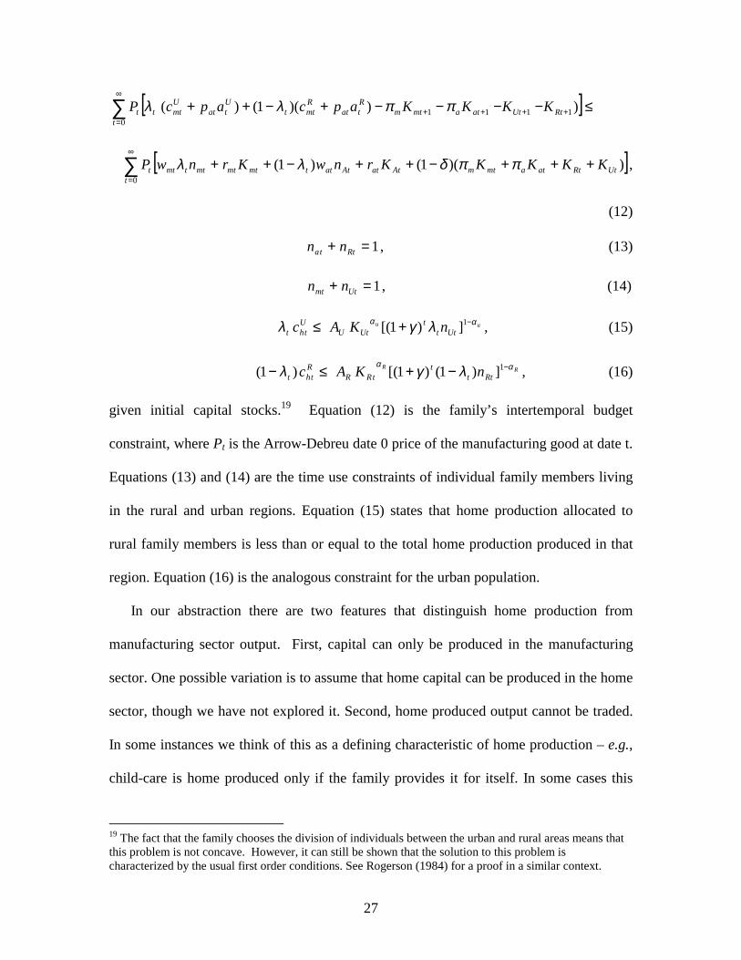
given initial capital stocks.19 Equation (12) is the family’s intertemporal budget
constraint, where Pt is the Arrow-Debreu date 0 price of the manufacturing good at date t.
Equations (13) and (14) are the time use constraints of individual family members living
in the rural and urban regions. Equation (15) states that home production allocated to
rural family members is less than or equal to the total home production produced in that
region. Equation (16) is the analogous constraint for the urban population.
In our abstraction there are two features that distinguish home production from
manufacturing sector output. First, capital can only be produced in the manufacturing
sector. One possible variation is to assume that home capital can be produced in the home
sector, though we have not explored it. Second, home produced output cannot be traded.
In some instances we think of this as a defining characteristic of home production – e.g.,
child-care is home produced only if the family provides it for itself. In some cases this
19 The fact that the family chooses the division of individuals between the urban and rural areas means that this problem is not concave. However, it can still be shown that the solution to this problem is characterized by the usual first order conditions. See Rogerson (1984) for a proof in a similar context.
28
assumption is probably not appropriate—for example, clothing made at home by family
members in the rural area may be sent to family members in the city. While our
assumption is extreme, what is important for our results is that for a significant
component of home production it is costly to transfer it across regions.
5.2 Quantitative Findings
In this section we examine the quantitative properties of the model extended to include
home production. The nature of the analysis is the same as in the previous model.
Namely, we calibrate the model economy to US time series data, and then introduce
distortions to the resource cost of capital used in market production.
Calibration
The set of observations used in the calibration includes all those used in Section 4, plus
the following 2 observations: the 1990 stock of household durables, and the fraction of
discretionary time spent in market work for individuals outside the agricultural sector.
The empirical counterparts of the model are the same as previous, and we now identify
investment in household capital as expenditures on consumer durables, and household
capital is thus the stock of household durables. We note that the empirical counterparts of
the residences of both farmers and non-farmers are included as part of the manufactured
capital stock, rather than as part of household capital.
The introduction of home production adds five parameters to the model: µ, ρ, α, AR,
and AU. The steps involved in calibrating the non-home production parameters follow
closely Section 4, and for this reason are not described here. As is evident by the fact that
we have only added 2 observations on first moments to our list of observations to be
29
matched, we must rely on some additional information to tie down values of the home
production parameters. It is not possible to identify the elasticity of substitution between
market and non-market consumption from first moments. Consequently, we rely on the
estimates of this parameter in the literature. Rupert et al. (1995) and McGrattan et al.
(1997) obtain estimates from micro data and macro data respectively in the range .40-.45.
Though we think that the relevant elasticity may be even slightly higher at low levels of
development we set ρ = .40 in our benchmark model.20 The values of the TFP parameters
affect the units in which output is measured. We are thus free to normalize one of these
two parameters to 1. We choose to assign AR = 1.0. As our premise is that TFP in home
production in the rural region is greater than its counterpart in the urban region, we set AU
= .90 in our benchmark specification. We will examine the sensitivity of our findings to
changes in AU. Having made these assignments, the two observations that we added can
be used to determine values for α and µ. The calibrated parameter values for our
benchmark model are reported in Table 3.
Before turning to the cross-country comparisons, we note that the introduction of
home production has relatively little effect on the implied time series for the United
States between 1870 and 1990 for aggregate output, investment, and consumption.
However, the model now has much richer predictions for time allocations. In the
previous model the only issue was what fraction of each agent's time endowment was
allocated to each of the two sectors. Now there is an allocation of individuals across the
20 The higher value for ρ corresponds to an assumption that home produced goods are more substitutable for market-produced non-agricultural goods in poor countries than in rich countries. In other words, home-produced goods are more similar to market-produced goods in poor countries than in rich countries. This seems entirely reasonable.
30
rural and urban regions, and within each region an allocation of time between market and
non-market activity.
Several interesting results emerge. First, and perhaps not surprisingly, given our
assumptions about home production possibilities, we find that individuals in the rural
region devote more of their time to home production than do workers in the urban region.
More interesting, our model predicts a decline in the fraction of time that an individual
spends in market work over the 120-year period. The decline in the workweek in
manufacturing is more than 10 percent, and virtually all of it takes place between 1870
and 1960. Hence, this model can account for a large part of the secular decline in the
workweek in manufacturing. In the agricultural sector the decline is even larger: the
workweek falls by almost 25 percent. Coincident with this secular decrease in time
devoted to market work, there is a large movement of workers from the rural to the urban
region. In 1870 the model predicts a rural share of 36 percent and by 1990 this share is
reduced to only 5 percent. This decline is somewhat smaller than what is found in the
data – from roughly 48 percent in 1870 to 4 percent in 1990. However, it is somewhat
larger than the decline we found in the model without home production.
Cross Country Comparisons
How does the introduction of home production possibilities affect the model’s predictions
for sectoral differences across rich and poor countries? In this section we repeat the
experiment whereby we introduce policy distortions and calculate the equilibrium path
for the distorted economy. In the interests of space we only report results for the case
where both the manufacturing and agricultural sector are subject to the same barrier. As
before we consider the case of π = 4. Table 4 shows these results. The table reports

31
NIPA GDP per capita (Y), agriculture’s share of GDP (paYa/Y), agriculture’s share of
employment (1-λ), relative productivity ))]1/(/()/[( λλ −≡ aaMam YpYyy , time
allocated to agriculture work in the rural sector (na), and time allocated to market work in
the manufacturing sector (nm) at various dates across the undistorted and distorted
economies. Note that our measure of relative productivity is chosen to correspond to the
concept used in the data. Specifically, it looks at output per worker and not output per
unit of labor input.
The introduction of home production improves the model’s ability to account for the
cross-country data along three dimensions. First, the model now generates much larger
differences in output. In fact, the difference in GDP per capita associated with a barrier of
4 is approximately the factor 30 observed across countries. Second the model now
predicts sizable differences in the share of employment accounted for by agriculture
across rich and poor countries in 1990. In the undistorted economy, agriculture’s share of
employment is 5 percent in 1990, while in the distorted economy its share is 63 percent.
Third, the model now generates large cross-country differences in sectoral relative
productivity. Relative productivity of the agricultural sector in the model is almost six
times larger in the undistorted economy than it is in the distorted economy in 1990. This
is actually very close to the difference between the richest and poorest countries in the
1990 cross-section.
The reason the model generates these large differences in relative productivity is that
there are large differences in time allocations of rural workers in 1990 across the rich
(undistorted) and poor (distorted) economies. Rural workers in the poor economy are
working only about 20% as much in market activity as their counterparts in a rich

32
economy. Differences in time allocations in the urban region are much less pronounced.
This asymmetry between the distortions on rural and urban time allocations is due to the
asymmetry of home production opportunities across rural and urban regions.
Recall that in the data it is unclear to what extent differences in relative sectoral
productivity reflect differences in real outputs or differences in prices. In our model we
can easily assess the role of these two factors. In the 1990 cross section consisting of the
distorted and undistorted economy, we find that the difference is accounted for almost
entirely by the difference in relative prices. That is, differences in real output per worker
in agriculture are roughly the same as differences in GDP per worker. Recall that the
model without home production predicted that differences in agricultural output per
worker were much less than differences in GDP per worker. Hence, the addition of home
production improves the model’s ability to account for the data along this additional
dimension.
As can be seen in the table, relative productivity differentials across distorted and
undistorted countries increase over time. This phenomenon is driven by the secular
change in time allocations of workers in the two regions. In the distorted economy the
secular decline in the (market) workweek in the rural region is much larger than in the
undistorted economy. Initially, although the distorted economy has more workers in the
rural region, workers in the distorted economy have roughly the same time allocations as
workers in the undistorted economy. This is because the subsistence constraint is
relatively binding. Over time, this constraint eases and the time allocation in the rural
area becomes increasingly distorted toward home production. Although the table stops in
1990 it is worth noting that the time allocation of rural workers to market production in

33
subsequent years in the distorted economy continues to show a decline, although at a
slower rate than over the 1870-1990 period. In the undistorted economy, in contrast, there
is no subsequent decline. As a result, the relative productivity differentials continue to
widen. Moreover, these differentials begin to reflect real output differences in agriculture.
The model also does a better job matching the differences in agriculture’s share of
output across rich and poor countries, although the differences predicted by the model are
still small relative to what is found in the data. One reason why the differences in
agriculture’s share of output implied by the model are so small is that individuals living
in the rural region in the distorted economy allocate a small fraction of their time to
market activities. A second reason is that the relative price of agriculture is lower in the
poorer country, by roughly 80 percent. Alternative specifications for preferences may
give rise to smaller effects on relative prices and help the model on this dimension.
Accounting for the large difference in agriculture’s share of GDP across rich and poor
countries is a matter for future work.
One other difference between the two economies is worth pointing out. A rather
surprising result is that measured output in the distorted economy grows at a much slower
rate than in the undistorted economy over the 120-year period, implying that relative
GDPs diverge for a long time. In fact, as Table 4 documents, it is not until roughly the
end of the sample period that the distorted economy displays a growth rate of real GDP
that is roughly equal to the exogenous growth rate of technology. This pattern is not
generated in the other models studied in this paper. It is, however, the pattern observed in
the data. With the start of the Industrial Revolution in England, disparities in living
standards between the world’s rich and poor countries began to increase. These

34
disparities continued to increase until 1950. Our research shows that one does not need to
assume differential rates of exogenous technological change or poverty traps to account
for this pattern. Instead, a two-sector version of the neoclassical growth model with home
production, a broad concept of capital, and a subsistence term can qualitatively generate
this pattern. We conclude that this model may be very useful in accounting for the
divergence in international incomes from the Industrial Revolution to the latter half of the
twentieth century.
Sensitivity to Alternative Values of AU
A key feature of our abstraction is that TFP is lower in urban home production than in
rural home production. In the numerical experiments, this was represented by a 10
percent productivity gap between rural and urban areas in home production. Given the
arbitrary nature of this parameterization, it is worthwhile to examine the sensitivity of the
model’s results to changes in this parameter value. We, therefore, consider alternative
values of .85, .95 and 1.00 for AU. In each case we recalibrate the model as discussed
previously and compute the equilibrium path for 120 years. In the interest of space we
only report statistics for 1990 rather than the entire time series.
Table 5 presents the results. Several features are worth noting. Starting with the case
with no relative productivity differences, we observe that the model still predicts large
differences in income across the two economies. However, it no longer predicts large
differences in relative sectoral productivities between rich and poor countries. As AU is
decreased several patterns emerge. First, the difference in income per capita increases.
Second, the difference in the share of the population living in the rural area increases.
And third, the difference in relative sectoral productivities also increases. The table also
35
indicates that the difference in agriculture’s share of GDP also increases, but this effect is
fairly modest. The qualitative patterns in this table are intuitive given the mechanics of
the model discussed earlier. We conclude from this that the model predictions that we are
emphasizing require relatively small productivity differences. Even with a differential of
.05 the model generates results that are quite different from the two-sector model without
home production.
Welfare Comparison
Lastly, we think it is instructive to examine some of the welfare implications of our
model. As discussed and analyzed in Parente et al. (2000), home production models
imply that differences in measured income across countries overstate the true differences
in well-being across countries.21 To give a sense of the overstatement, we note that in our
benchmark specification, in 1990, the undistorted economy consumes roughly 33 times
more of the manufactured consumption good than does the distorted economy, 1.1 times
more of the agricultural good, but only about two-thirds as much home produced output.
In what follows we use our model to give a more precise measure of actual welfare
differences and contrast them to those obtained in models without home production.
We begin with the standard one-sector growth model described in Section 3 of this
paper. We shall assume a parameterization that roughly accords with the values used in
Sections 4 and 5 for parameters θ , δ , and β, and a barrier π such that the factor
difference in relative steady state incomes in this model equals the factor difference of
33 we obtained in our benchmark specification for 1990. Given θ = 2/3, the
corresponding value of π is 5.75.
36
We now describe our procedure to compute the welfare gain associated with
removing the barrier. We note that our measure is not affected by monotone
transformations of the utility function. We begin by first computing the equilibrium path
that would result if an economy beginning in the steady state corresponding to π = 5.75
eliminates this barrier. We next compute the utility of the representative agent associated
with this equilibrium path. We also compute the utility of the representative agent if the
economy does not eliminate this barrier and it remains in the steady state corresponding
to π = 5.75. We then ask by what factor would we have to increase consumption in each
period under this second scenario in order that the resulting lifetime utility equal that
achieved when the barrier were removed.
The number we obtain in this procedure is 2.8; i.e., if consumption were to be
increased by a factor of 2.8 the individual would be indifferent about removing the
barrier. Note that this number is small in comparison to the differences in steady state
consumptions. The ratio of the two consumptions across the two steady states is 33 – the
same as the ratio of the two outputs. The fact that our compensating differential is so
much smaller than this factor indicates the importance of allowing for the accumulation
of capital needed to reach the new steady state.
We now repeat this calculation in the context of our two-sector growth model with
home production. That is, we assess the gain in utility that the individuals in the poor
economy would experience if the distortion were removed, taking the starting point as the
1990 allocations in the distorted economy. After computing the resulting equilibrium and
the lifetime utility of the representative family, we then ask by what factor would we
21 Note that we have also assumed that there is unmeasured investment in the economy. This will not matter for our welfare calculations since they are based on consumption flows.
37
have to increase consumption in each period in the economy that does not remover the
barriers in order to make the lifetime family utilities the same between economies. In
calculating this factor increase, we assume the consumption of all family members is
increased proportionately. The number we obtain is 1.9, which is about two-thirds of the
number we obtained in the welfare calculation for the one-sector growth model with no
home production. We conclude from this that while home production does diminish the
welfare differences between rich and poor countries for a given difference in measured
output, the reduction is not particularly large.
6. Conclusion
Development economists have long noted the importance of agriculture in the share of
economic activity in poor countries. Contemporary researchers working with applied
general equilibrium models almost always abstract from sectoral issues. In this paper, we
introduced agriculture into the neoclassical growth model and examined the implications
for international incomes and sectoral patterns. We found that a straightforward extension
of the model fails to account for key sectoral differences observed across rich and poor
countries. This failure led us to consider an extension of the model that incorporates
home production. The key implication of this model is that distortions to capital
accumulation lead to a relative increase in the amount of unmeasured activity taking
place in rural areas. A reduction of the distortions leads to an efficiency-enhancing
reallocation of inputs plus an increase in measured economic activity. We found the
model accounts for a number of features of the sectoral transformation observed in
economic data, both in the cross section and the time series.
38
References
Bautista, Romeo and Alberto Valdés. 1993. The Bias Against Agriculture: Trade and Macroeconomic Policies in Developing Countries. San Francisco: A Copublication of the International Center for Economic Growth and the International Food Policy Research Institute, with ICS Press.
Caselli, Francesco and Wilbur John Coleman II. 1998. How regions converge. Manuscript:
Graduate School of Business, University of Chicago. Chari, V.V., Patrick Kehoe, and Ellen McGrattan. 1996. The poverty of nations: A
quantitative exploration.” NBER Working Paper 5414. Chenery, H.B. and M. Syrquin. 1975. Patterns of Development, 1950-1970. London: Oxford
University Press. Collins, W. and J. Williamson. 1999 . “Capital goods prices, global capital markets and
accumulation: 1870-1950.” NBER Working Paper No. 7145. Cooley, Thomas F. and Edward C. Prescott. Economic growth and business cycles. Chapter 1
in Frontiers of Business Cycle Research, ed. Thomas F. Cooley. Princeton, New Jersey: Princeton University Press.
Echevvaria, Cristina. 1995. Agricultural development vs. industrialization: Effects of trade.
Canadian Journal of Economics 28 (3): 631-47. Echevarria, Cristina. 1997. Changes in sectoral composition associated with economic growth.
International Economic Review 38 (2): 431-52. Fei, John C. H. and Gustav Ranis. 1964. Development of the Labor Surplus Economy: Theory
and Policy. A Publication of the Economic Growth Center, Yale University. Homewood, Illinois: Richard D. Irwin, Inc.
Hall, Robert E. and Charles I. Jones. 1999. Why do some countries produce so much more
output per worker than others? Quarterly Journal of Economics 114 (1): 83-116. Hayami, Yujiro and Vernon W. Ruttan. 1985. Agricultural Development: An International
Perspective. Baltimore: Johns Hopkins University Press. Inada, K. 1963. On a two-sector model of economic growth: Comments and a generalization.
Review of Economic Studies 30 (June): 95-104 Johnston, Bruce F. and John W. Mellor. 1961. The role of agriculture in economic
development. American Economic Review 51(4): 566-93. Johnston, Bruce F. and Peter Kilby. 1975. Agriculture and Structural Transformation:
Economic Strategies in Late-Developing Countries. New York: Oxford University Press. Jones, Charles I. 1994. “Economic growth and the relative price of capital.” Journal of
Monetary Economics 34:359-382.

39
Klenow, Peter and Andres Rodriguez-Clare. 1997. The neoclassical revival in growth
economics: Has it gone too far? In Ben S. Bernanke and Julio J. Rotemberg, eds., NBER Macroeconomics Annual 1997. Cambridge, MA: MIT Press.
Kurian, George Thomas. 1994. Datapedia of the United States 1790-2000: America Year by
Year. Lanham, MD: Bernan Press. Kuznets, Simon. 1946. National Income: A Summary of Findings. New York: NBER. __________ 1966. Modern Economic Growth. New Haven: Yale University Press. __________ 1971. Economic Growth of Nations. Harvard University Press, Cambridge USA. Kongsamut, Piyabha, Sergio Rebelo, and Danyang Xie. 1997. Beyond balanced growth.
NBER Working Paper 6159. Krueger, Anne O., Schiff, Maurice and Alberto Valdes. 1992. The Political Economy of
Agricultural Pricing Policy (Volumes I-III). A World Bank Comparative Study. Baltimore: Published for the World Bank by Johns Hopkins University Press.
Laitner, John. 1998. Structural change and economic growth. Manuscript: Department of
Economics, University of Michigan. Maddison, Angus. 1995. Monitoring the World Economy: 1820-1992. Paris: Development
Centre of the OECD. Mankiw, N. Gregory, David Romer, and David N. Weil. 1992. A contribution to the empirics
of economic growth. Quarterly Journal of Economics 107 (2): 407-37. Matsuyama, Kiminori. 1992 Agricultural productivity, comparative advantage, and economic
growth. Journal of Economic Theory 58 (2): 317-34. Mellor, John W. 1986. Agriculture on the road to industrialization. In Development
Studies Reconsidered, ed. John P. Lewis and Valeriana Kallab. Washington DC: Overseas Development Council.
Mitchell, B.R. 1992. International Historical Statistics: Europe 1750-1988. New York: Stockton Press.
Mitchell, B.R. 1993. International Historical Statistics: The Americas 1750-1988. New York:
Stockton Press. Mitchell, B.R. 1995. International Historical Statistics: Africa, Asia & Oceania 1750-1988.
New York: Stockton Press. Musgrave, John. Fixed reproducible tangible wealth in the United States: Revised
estimates for 1990-92 and summary estimates for 1925-92. Survey of Current Business (September 1993), 61-69.

40
Parente, Stephen and Edward C. Prescott. 1994. Barriers to technology adoption and
development. Journal of Political Economy 102 (2): 298-321. Parente, Stephen and Edward C. Prescott. 2000. The Barrier to Riches. Cambridge: MIT
Press. Parente, Stephen L., Richard Rogerson, and Randall Wright. 2000. Home work in
development economics: home production and the wealth of nations, forthcoming in Journal of Political Economy.
Prescott, Edward C. 1998. Needed: a theory of total factor productivity. International Economic
Review 39 (3) 525-51. Prasada Rao, D.S. 1993. Intercountry comparisons of agricultural output and productivity. FAO
Economic and Social Development Paper 112. Rome: Food and Agriculture Organization of the United Nations.
Restuccia, Diego and Carlos Urrutia. 2000. Relative prices and investment rates, forthcoming
in Journal of Monetary Economics Rogerson, Richard. 1984. “Topics in the Theory of Labor Markets.” Unpublished Ph.D.
dissertation, University of Minnesota. Rupert, Peter, Richard Rogerson, and Randall Wright. 1995. Estimating substitution
elasticities in household production models. Economic Theory 6 (1) 179-193. Schiff, Maurice and Alberto Valdes. 1992. The Political Economy of Agricultural Pricing
Policy (Volume 4: A Synthesis of the Economics in Developing Countries). A World Bank Comparative Study. Baltimore: Published for the World Bank by Johns Hopkins University Press.
Schultz, T. W. 1964. Transforming Traditional Agriculture. New Haven: Yale University Press. Syrquin, Moshe. 1988. Patterns of structural change. Chapter 7 in Handbook of Development
Economics, Vol. I, ed. H. Chenery and T.N. Srinivasan. Amsterdam: Elsevier Science Publishers.
Takayama, A. 1963. On a two-sector model of economic growth: A comparative static analysis.
Review of Economic Studies 30 (June): 95-104. Timmer, C. Peter. 1988. The agricultural transformation. Chapter 8 in Handbook of
Development Economics, Vol. I, ed. H. Chenery and T.N. Srinivasan. Amsterdam: Elsevier Science Publishers.

41
U.S. Department of Commerce, Bureau of the Census. 1975. Historical Statistics of the United States: Colonial Times to 1970. Washington, DC: U.S. Bureau of the Census.
Uzawa, H. 1961. On a two-sector model of economic growth: I. Review of Economic Studies 29
(October): 40-47. Uzawa, H. 1963. On a two-sector model of economic growth: II. Review of Economic Studies 30
(June): 105-118.
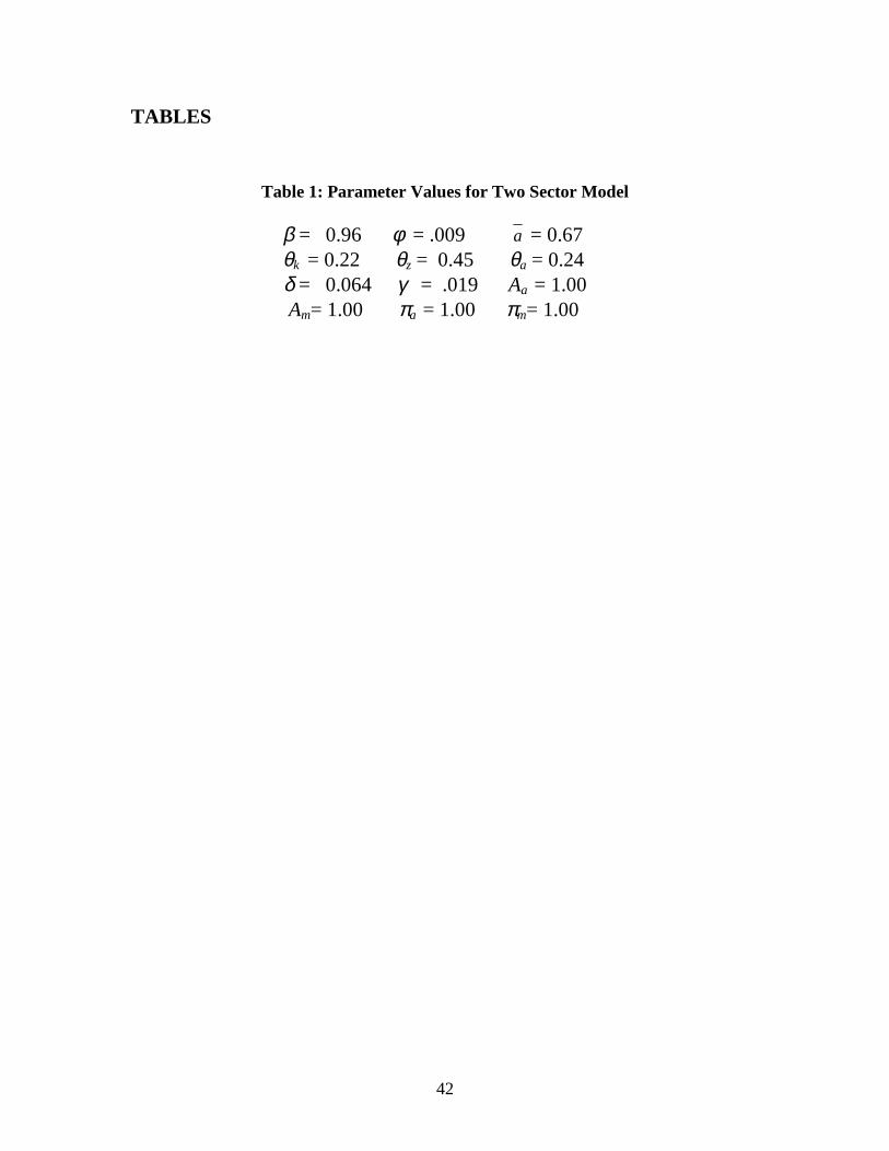
42
TABLES
Table 1: Parameter Values for Two Sector Model
β = 0.96 φ = .009 a = 0.67 θk = 0.22 θz = 0.45 θa = 0.24 δ = 0.064 γ = .019 Aa = 1.00 Am= 1.00 πa = 1.00 πm= 1.00
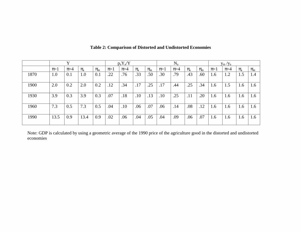
Table 2: Comparison of Distorted and Undistorted Economies
Y paYa/Y Na ym /ya π=1 π=4 πa πm π=1 π=4 πa πm π=1 π=4 πa πm π=1 π=4 πa πm 1870
1.0 0.1 1.0 0.1 .22 .76 .33 .50 .30 .79 .43 .60 1.6 1.2 1.5 1.4
1900
2.0 0.2 2.0 0.2 .12 .34 .17 .25 .17 .44 .25 .34 1.6 1.5 1.6 1.6
1930
3.9 0.3 3.9 0.3 .07 .18 .10 .13 .10 .25 .11 .20 1.6 1.6 1.6 1.6
1960
7.3 0.5 7.3 0.5 .04 .10 .06 .07 .06 .14 .08 .12 1.6 1.6 1.6 1.6
1990
13.5 0.9 13.4 0.9 .02 .06 .04 .05 .04 .09 .06 .07 1.6 1.6 1.6 1.6
Note: GDP is calculated by using a geometric average of the 1990 price of the agriculture good in the distorted and undistorted economies


Table 3: Parameter Values, Home Production Model
β = 0.96 ρ = 0.40 µ = 0.36 φ = 0.003 a = 0.39 θm = 0.67 θa = 0.24 α = 0.11 δ = 0.063 γ = .0198 AR = 1.00 AU =0.90 πm = 1.0 πa = 1.0
Table 4. International Comparisons Home Production
GDP paYa/GDP 1-λ ym /ya na nm π=1 π=4 π=1 π=4 π=1 π=4 π=1 π=4 π=1 π=4 π=1 π=4 1870 1.00 0.12 .22 .68 .36 .83 1.90 2.32 .58 .68 .64 .70 1900 1.92 0.14 .13 .49 .22 .74 2.03 2.97 .52 .42 .60 .51 1930 3.91 0.18 .07 .32 .14 .67 2.13 4.36 .48 .26 .57 .43 1960 7.31 0.27 .04 .19 .08 .63 2.20 7.36 .46 .16 .55 .40 1990 13.4 0.41 .02 .12 .05 .63 2.26 12.9 .44 .09 .55 .39 Note: GDP is calculated by using a geometric average of the 1990 price of the agriculture good in the distorted and undistorted economies
Table 5: Sensitivity of Results to Value of TFP in Urban Home Production (1990 Comparisons)
GDP paYa/GDP 1-λ ym /ya na nm Au π=1 π =4 π=1 π=4 π=1 π=4 π=1 π =4 π=1 π =4 π=1 π=4 .85 13.3 .36 .02 .13 .06 .72 2.9 17.5 .37 .08 .55 .44. .90 13.4 .41 .02 .12 .05 .63 2.3 12.9 .44 .09 .55 .39 .95 13.2 .46 .02 .11 .04 .43 1.9 6.5 .50 .13 .55 .31 1.00 13.2 .53 .02 .11 .04 .19 1.6 1.9 .55 .27 .55 .25

FIGURES
Figure 1: Fraction of GDP in agriculture, 1990 cross-section
1/81/161/32 1/4 11/20
0.1
0.2
0.3
0.4
0.5
0.6
Real per capita GDP relative to US
Fra
ctio
n of
GD
P
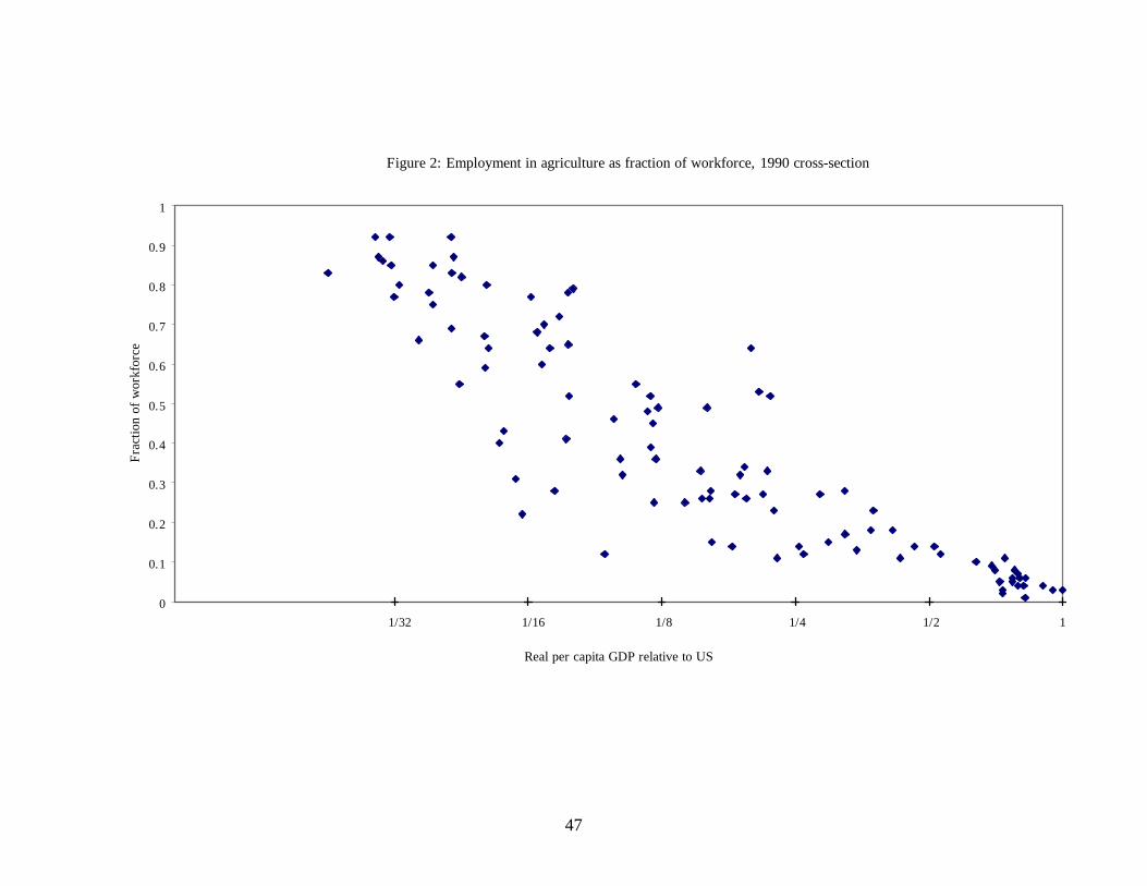
47
Figure 2: Employment in agriculture as fraction of workforce, 1990 cross-section
1/81/161/32 1/2 11/4
0
0.1
0.2
0.3
0.4
0.5
0.6
0.7
0.8
0.9
1
Real per capita GDP relative to US
Fra
ctio
n of
wor
kfor
ce
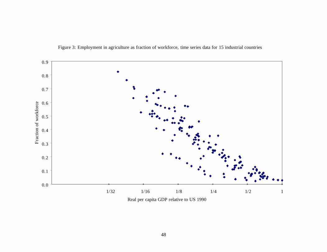
48
Figure 3: Employment in agriculture as fraction of workforce, time series data for 15 industrial countries
1/21/41/81/161/32 10.0
0.1
0.2
0.3
0.4
0.5
0.6
0.7
0.8
0.9
Real per capita GDP relative to US 1990
Fra
ctio
n of
wor
kfor
ce

49
Figure 4: Agriculture share of GDP, time series data for 15 industrial countries
1/21/41/81/161/32 10.0
0.1
0.2
0.3
0.4
0.5
0.6
0.7
Real per capita GDP relative to US 1990
Fra
ctio
n of
GD
P
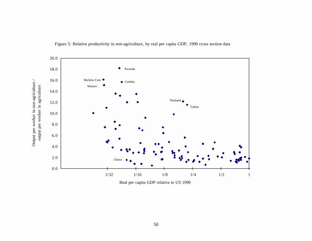
50
Figure 5: Relative productivity in non-agriculture, by real per capita GDP, 1990 cross section data
1/21/41/81/161/32 10.0
2.0
4.0
6.0
8.0
10.0
12.0
14.0
16.0
18.0
20.0
Real per capita GDP relative to US 1990
Out
put p
er w
orke
r in
non
-agr
icul
ture
/
outp
ut p
er w
orke
r in
agr
icul
ture
Rwanda
GambiaBurkina Faso
Malawi
Thailand
Gabon
Ghana
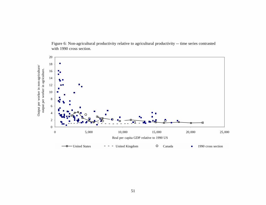
51
Figure 6: Non-agricultural productivity relative to agricultural productivity -- time series contrasted with 1990 cross section.
0
2
4
6
8
10
12
14
16
18
20
0 5,000 10,000 15,000 20,000 25,000
Real per capita GDP relative to 1990 US
Out
put p
er w
orke
r in
non
-agr
icul
ture
/ou
tput
per
wor
ker
in a
gric
ultu
re.
United States United Kingdom Canada 1990 cross section
Recommended