Final Presentation of the Project, 21 Jan 2010 1
Uncertainty estimates and guidance for road transport emission calculationsA JRC/IES project performed by EMISIA SA
Leon NtziachristosLaboratory of Applied Thermodynamics, Aristotle University Thessaloniki
Charis Kouridis, Dimitrios Gktazoflias, Ioannis KioutsioukisEMISIA SA, ThessalonikiPenny DilaraJRC, Transport and Air Quality Unit
http://ies.jrc.ec.europa.eu/
http://www.jrc.ec.europa.eu/[email protected]

Final Presentation of the Project, 21 Jan 2010 2
Project ID
• Project was initiated Dec. 17, 2008 with an official duration of 9 months
• Objectives:– Evaluate the uncertainty linked with the various input
parameters of the COPERT 4 model,– Assess the uncertainty of road transport emissions in two
test cases, at national level,– Include these uncertainty estimates in the COPERT 4
model, and– Prepare guidance on the assessment of uncertainty for the
Tier 3 methods (COPERT 4).
Final Presentation of the Project, 21 Jan 2010 3
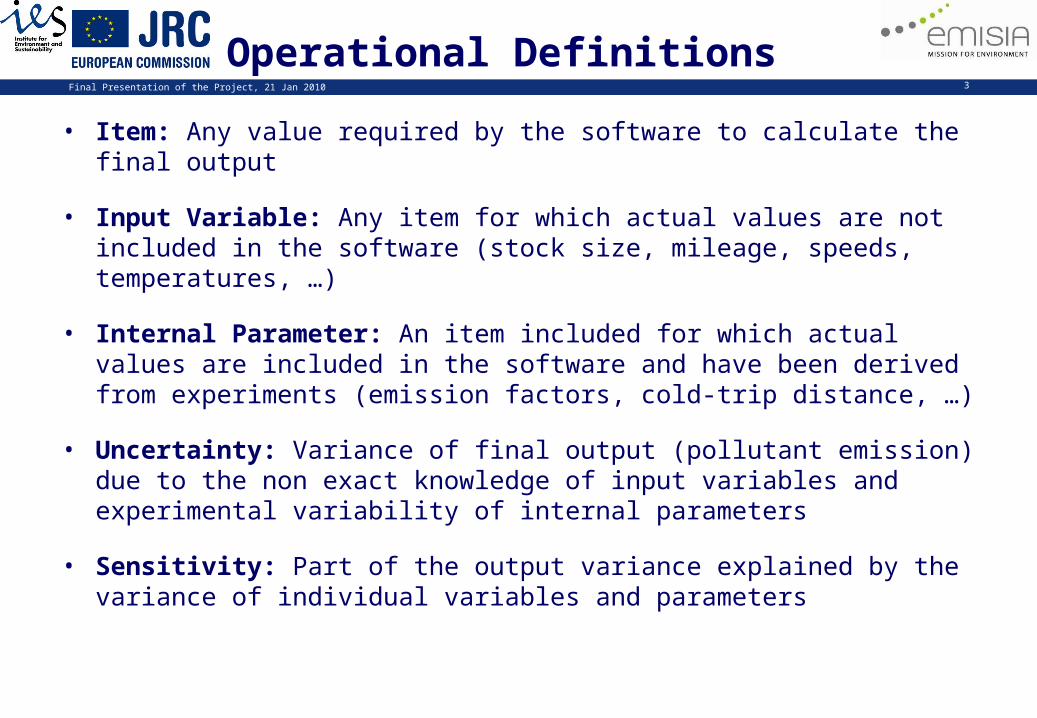
Operational Definitions
• Item: Any value required by the software to calculate the final output
• Input Variable: Any item for which actual values are not included in the software (stock size, mileage, speeds, temperatures, …)
• Internal Parameter: An item included for which actual values are included in the software and have been derived from experiments (emission factors, cold-trip distance, …)
• Uncertainty: Variance of final output (pollutant emission) due to the non exact knowledge of input variables and experimental variability of internal parameters
• Sensitivity: Part of the output variance explained by the variance of individual variables and parameters
Final Presentation of the Project, 21 Jan 2010 4
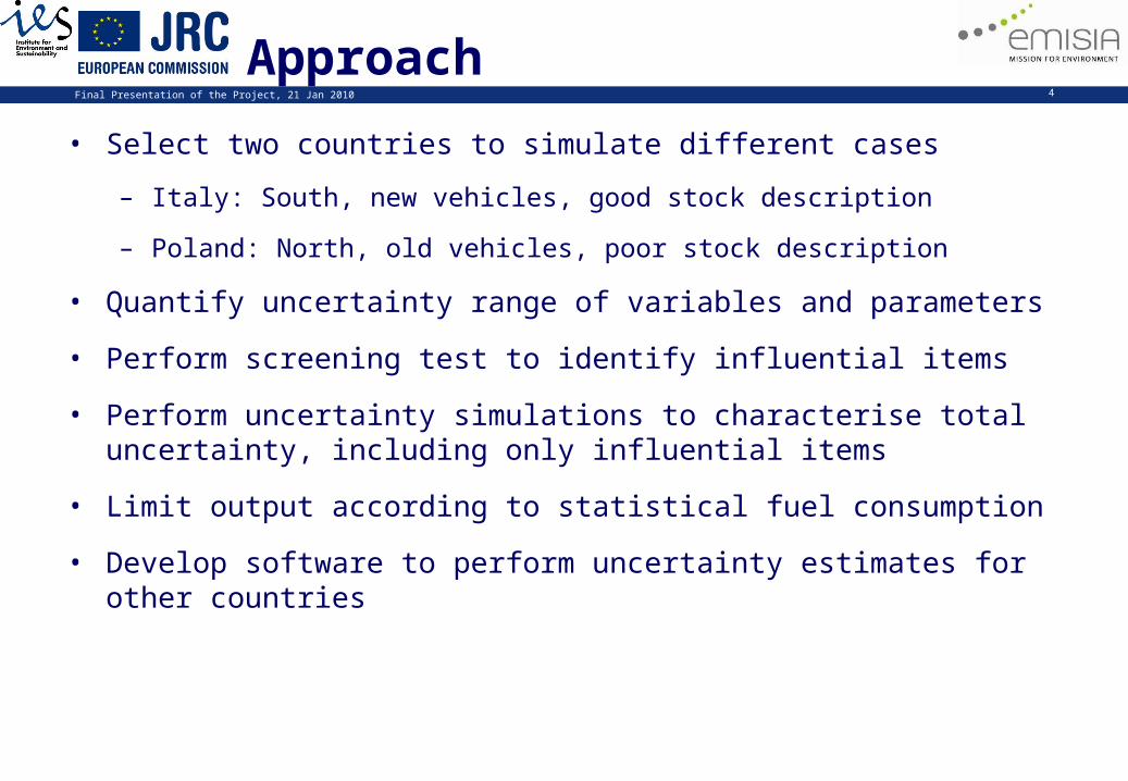
Approach
• Select two countries to simulate different cases
– Italy: South, new vehicles, good stock description
– Poland: North, old vehicles, poor stock description
• Quantify uncertainty range of variables and parameters
• Perform screening test to identify influential items
• Perform uncertainty simulations to characterise total uncertainty, including only influential items
• Limit output according to statistical fuel consumption
• Develop software to perform uncertainty estimates for other countries

Final Presentation of the Project, 21 Jan 2010 5
Items for which uncertainty has been assessed
Item Description Item Description
Ncat Vehicle population at category level LFHDV Load Factor
NsubVehicle population at sub-category level
tminAverage min monthly temperature
NtechVehicle population at technology level
tmaxAverage max monthly temperature
Mtech Annual mileage Mm,tech Mean fleet mileage
UStech Urban share RVP Fuel reid vapour pressure
Hstech Highway share H:C Hydrogen-to-carbon ratio
RStech Rural share O:C Oxygen-to-carbon ratio
USPtech Urban speed S Sulfur level in fuel
HSPtech Highway speed ehot,tech Hot emission factor
RSPtech Rural speed ecold/ehot,tech Cold-start emission factor
Ltrip Mean trip length b Cold-trip distance

Final Presentation of the Project, 21 Jan 2010 6
Variance of the total stock
ITALYACEA ACEM ACI Eurostat
μ σ2005 2005 2005 2005
Passenger Cars 34 667 485 34 667 485 34 636 400 34 657 123 17 947
Light Duty Vehicles 3 257 525 3 633 900 3 445 713 266 137
Heavy Duty Vehicles 1 070 308 958 400 1 014 354 79 131
Buses 94 437 94 437 94 100 94 325 195
Mopeds 5 325 000 4 560 907 4 942 954 540 295
Motorcycles 4 938 359 4 938 359 4 933 600 4 936 773 2 748
POLANDACEA ACEM Poland Stat Eurostat
μ σ2005 2005 2005 2005
Passenger Cars 12 339 353 12 339 000 12 339 000 12 339 118 204
Light Duty Vehicles 1 717 435 2 304 500 2 178 000 2 066 645 308 968
Heavy Duty Vehicles 587 070 737 000 662 035 106 017
Buses 79 567 79 600 80 000 79 722 241
Mopeds 337 511 337 511 0
Motorcycles 753 648 754 000 753 824 249

Final Presentation of the Project, 21 Jan 2010 7
Subsector variance Italy
Sector Subsector Known Values Unknown valuesPassenger Cars Gasoline <1,4 l 18.025.703 627Passenger Cars Gasoline 1,4 - 2,0 l 5.090.465Passenger Cars Gasoline >2,0 l 408.278Passenger Cars Diesel <2,0 l 7.987.956 145Passenger Cars Diesel >2,0 l 1.822.935Passenger Cars LPGPassenger Cars 2-StrokeLight Duty Vehicles Gasoline <3,5t 280.005 7.580Heavy Duty Vehicles Gasoline >3,5 t 4.343Light Duty Vehicles Diesel <3,5 t 2.695.478 35.174Heavy Duty Vehicles Diesel 3,5 - 7,5 t 190.842Heavy Duty Vehicles Diesel 7,5 - 16 t 187.804Heavy Duty Vehicles Diesel 16 - 32 t 206.345Heavy Duty Vehicles Diesel >32t 1.905Buses Urban Buses 2.281 92Buses Coaches 66.548Mopeds <50 cm³Motorcycles 2-stroke >50 cm³ 1.397.575 927Motorcycles 4-stroke <250 cm³ 1.545.423Motorcycles 4-stroke 250 - 750 cm³ 1.488.571Motorcycles 4-stroke >750 cm³ 505.863
Standard deviation is produced by allocating the unknown values to the smaller class, the larger class and uniformly between classes

Final Presentation of the Project, 21 Jan 2010 8
Subsector variance Poland
Sector Subsector μ σ
Passenger Cars Gasoline <1,4 l 5.890.018 194.212
Passenger Cars Gasoline 1,4 - 2,0 l 2.853.116 187.552
Passenger Cars Gasoline >2,0 l 253.264 38.415
Passenger Cars Diesel <2,0 l 1.660.117 113.710
Passenger Cars Diesel >2,0 l 314.139 60.785
Passenger Cars LPG 992.755 231.352
Light Duty Vehicles Gasoline <3,5t 980.551 9.244,7Heavy Duty Trucks Gasoline >3,5 t 108.400 1.022,0Light Duty Vehicles Diesel <3,5 t 732.359 7.323,6Heavy Duty Trucks Rigid <=7,5 t 73.538 5.147,7Heavy Duty Trucks Rigid 7,5 - 12 t 53.445 3.741,1Heavy Duty Trucks Rigid 12 - 14 t 25.422 1.779,5Heavy Duty Trucks Rigid 14 - 20 t 31.993 2.239,5Heavy Duty Trucks Rigid 20 - 26 t 28.597 2.001,8Heavy Duty Trucks Rigid 26 - 28 t 7.342 513,9Heavy Duty Trucks Rigid 28 - 32 t 8.928 625,0Heavy Duty Trucks Rigid >32 t 10.925 764,7Heavy Duty Trucks Articulated 14 - 20 t 10.741 751,8Heavy Duty Trucks Articulated 20 - 28 t 9.284 649,9Heavy Duty Trucks Articulated 28 - 34 t 15.037 1.052,6Heavy Duty Trucks Articulated 34 - 40 t 35.608 2.492,6Heavy Duty Trucks Articulated 40 - 50 t 8.083 565,8Heavy Duty Trucks Articulated 50 - 60 t 3.461 242,3Buses Urban Buses Midi <=15 t 1.813 126,9Buses Urban Buses Standard 15 - 18 t 35.035 2.452,5Buses Urban Buses Articulated >18 t 25.575 1.790,3Buses Coaches Standard <=18 t 15.944 1.116,0Buses Coaches Articulated >18 t 2.216 155,1Mopeds <50 cm³ 337.511 0,0Motorcycles 2-stroke >50 cm³ 454.508 31.815,5Motorcycles 4-stroke <250 cm³ 75.694 5.298,6Motorcycles 4-stroke 250 - 750 cm³ 128.674 9.007,2Motorcycles 4-stroke >750 cm³ 94.124 6.588,7
Poland Passenger cars: standard deviation calculated as one third of the difference between national statistics and FLEETS
Light Duty Vehicles: uncertainty of stock proportionally allocated to stock of diesel and gasoline trucks.
Other vehicle categories: standard deviation was estimated as 7% of the average (assumption).

Final Presentation of the Project, 21 Jan 2010 9
Technology classification variance – 1(2)
• Italy: Exact technology classification
• Poland: Technology classification varying, depended on variable scrappage rate
Gasoline PC <1,4 l
0,3
0,4
0,5
0,6
0,7
0,8
0,9
1,0
0 5 10 15 20age
φ(a
ge
)
G<1,4Alt1Alt2Alt3
Boundaries Introduced:
Age of five years: ±5 perc.units
Age of fifteen years: ±10 perc.units
All scrappage rates respecting boundaries are accepted → these induce uncertainty
100 pairs finally selected by selecting percentiles

Final Presentation of the Project, 21 Jan 2010 10
Fleet Breakdown Model
• The stock at technology level is calculated top-down by a fleet breakdown model (FBM), in order to respect total uncertainty at sector, subsector and technology level.
• That is, the final stock variance should be such as not to violate any of the given uncertainties at any stock level.
• The FBM operates on the basis of dimensionless parameters to steer the stock distribution to the different levels. Details in the report, p.44.

Final Presentation of the Project, 21 Jan 2010 11
Example of technology classification variance
• Example for GPC<1.4 l Poland
• Standard deviation: 3.7%, i.e. 95% confidence interval is ±11%
PC Gasoline<1,4 EURO 1
0 16
323
1 099
1 706 1 708
1 073
320
28 00
200
400
600
800
1 000
1 200
1 400
1 600
1 800
2 000
755
- 780
780
- 805
805
- 830
830
- 855
855
- 880
880
- 905
905
- 930
930
- 955
955
- 980
980
- 1,0
50
Number of vehicles (thousands)
Fre
qu
en
cy

Final Presentation of the Project, 21 Jan 2010 12
Emission Factor Uncertainty
• Emission factor functions are derived from several experimental measurements over speed
• (Example Gasoline Euro 3 cars)

Final Presentation of the Project, 21 Jan 2010 13
Performance of Individual Vehicles
0
0.2
0.4
0.6
0.8
1
1.2
0 20 40 60 80 100 120 140
average speed [km/h]
HC
[g
/km
]
Iveco 35/10 VW LT 35 Iveco 35-10 Turbo Daily Mercedes-Benz 210D
Mercedes-Benz 208D VW T4 Diesel VW LT 35 2 Ford Transit 120 2.5 TD

Final Presentation of the Project, 21 Jan 2010 14
Emission Factor Uncertainty
• Fourteen speed classes distinguished from 0 km/h to 140 km/h

Final Presentation of the Project, 21 Jan 2010 15
Emission Factor Uncertainty
• A lognormal distribution is fit per speed class, derived by the experimental data. Parameters for the lognormal distribution are given for all pollutants and all vehicle technologies in the Annex A of the report.

Final Presentation of the Project, 21 Jan 2010 16
Mileage Uncertainty – M0
• Mileage is a function of vehicle age and is calculated as the product of mileage at age 0 (M0) and a decreasing function of age:
• M0 was fixed for Italy based on experimental data• M0 was variable for Poland (s=0.1*M0) due to no
experimental data available
mb
m
m
T
bageage exp)(
0)()( MageageM tech

Final Presentation of the Project, 21 Jan 2010 17
Mileage Uncertainty – Age
• The uncertainty in the decreasing mileage function with age was assessed by utilizing data from all countries (8 countries of EU15)
• The boundaries are the extents from the countries that submitted data• Bm and Tm samples were selected for all curves that respected the
boundaries
PC Gasoline <1,4l
0,0
0,1
0,2
0,3
0,4
0,5
0,6
0,7
0,8
0,9
1,0
0 10 20 30 40age
φ (
ag
e)
minmaxAlt1Alt2Alt3

Final Presentation of the Project, 21 Jan 2010 18
Other variables - temperature
• Uncertainty of other variables was quantified based on literature data where available or best guess assumptions, when no data were available.
• Models were built for the temperature distribution over the months for the two countries.

Final Presentation of the Project, 21 Jan 2010 19
Statistical approach
1. Prepare the Monte Carlo sample for the screening experiment using the Morris design.
2. Execute the Monte Carlo simulations and collect the results.3. Compute the sensitivity measures corresponding to the elementary
effects in order to isolate the non-influential inputs.4. Prepare the Monte Carlo sample for the variance-based sensitivity
analysis, for the influential variables identified important in the previous step.
5. Execute the Monte Carlo simulations and collect the results 6. Quantify the importance of the uncertain inputs, taken singularly as
well as their interactions.7. Determine the input factors that are most responsible for producing
model outputs within the targeted bounds of fuel consumption.
Final Presentation of the Project, 21 Jan 2010 20
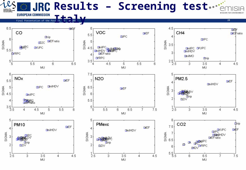
Results – Screening test Italy

Final Presentation of the Project, 21 Jan 2010 21
Results – Screening test Poland

Final Presentation of the Project, 21 Jan 2010 22
Results – Influential VariablesVariable Significant for Italy Significant for Poland
Hot emission factor
Cold overemission
Mean trip distance
Oxygen to carbon ratio in the fuel
Population of passenger cars -
Population of light duty vehicles
Population of heavy duty vehicles
Population of mopeds -
Annual mileage of passenger cars
Annual mileage of light duty vehicles
Annual mileage of heavy duty vehicles
Annual mileage of urban busses -
Annual mileage of mopeds/motorcycles -
Urban passenger car speed
Highway passenger car speed -
Rural passenger car speed -
Urban speed of light duty vehicles -
Urban share of passenger cars -
Urban speed of light duty vehicles -
Urban speed of busses -
Annual mileage of vehicles at the year of their registration -
The split between diesel and gasoline cars -
Split of vehicles to capacity and weight classes -
Allocation to different technology classes -

Final Presentation of the Project, 21 Jan 2010 23
Results – total uncertainty Italy w/o fuel correction
Final Presentation of the Project, 21 Jan 2010 24
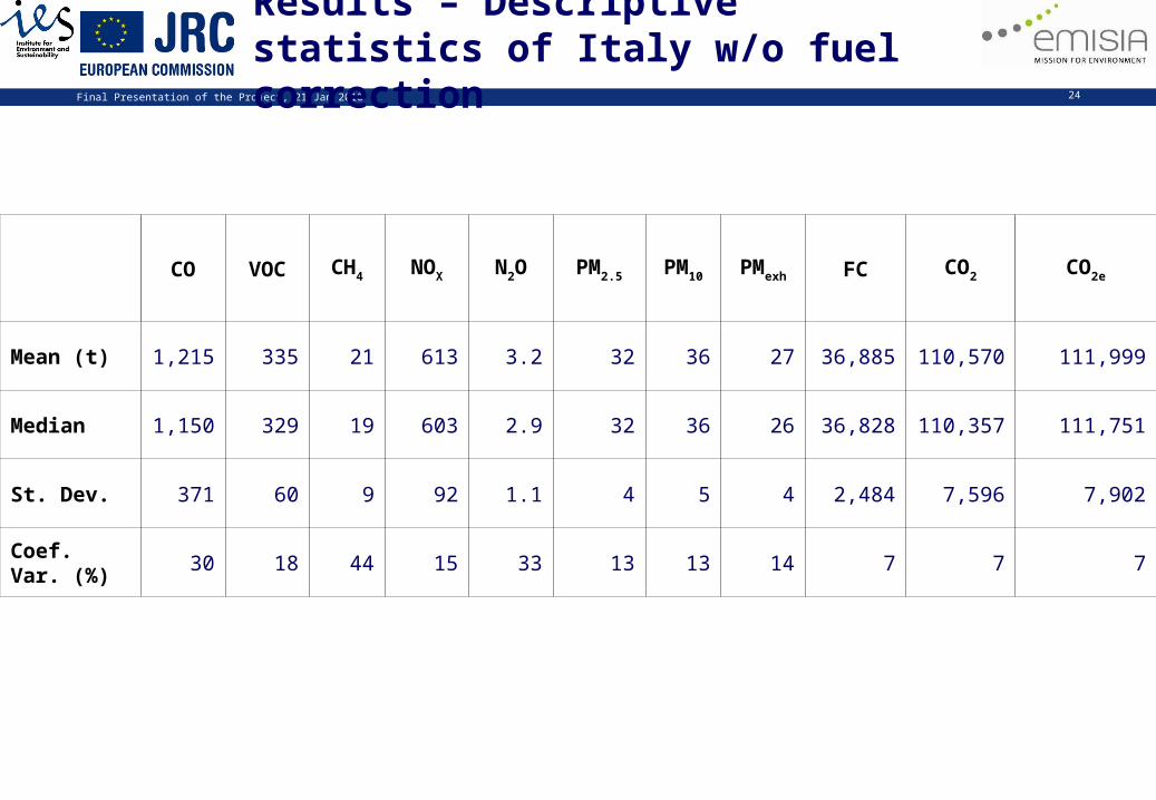
Results – Descriptive statistics of Italy w/o fuel correction
CO VOC CH4 NOX N2O PM2.5 PM10 PMexh FC CO2 CO2e
Mean (t) 1,215 335 21 613 3.2 32 36 27 36,885 110,570 111,999
Median 1,150 329 19 603 2.9 32 36 26 36,828 110,357 111,751
St. Dev. 371 60 9 92 1.1 4 5 4 2,484 7,596 7,902
Coef. Var. (%)
30 18 44 15 33 13 13 14 7 7 7

Final Presentation of the Project, 21 Jan 2010 25
Results – Necessary fuel correction for Italy
Unfiltered dataset: Std Dev = 7% of mean Filtered dataset: 3 Std Dev = 7% of mean

Final Presentation of the Project, 21 Jan 2010 26
Correction of sample required
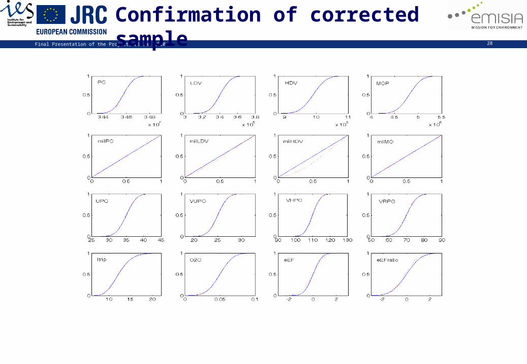
• Cumulative distributions of unfiltered (red) and of filtered (blue) datasets
• eEF, milHDV and milLDV are not equivalent• A corrected dataset was built to respect the fuel consumption induced
limitations

Final Presentation of the Project, 21 Jan 2010 27
Results – total uncertainty Italy with corrected sample
Final Presentation of the Project, 21 Jan 2010 28
Confirmation of corrected sample

Final Presentation of the Project, 21 Jan 2010 29
Results – Descriptive statistics of Italy with corrected sample
CO VOC CH4 NOx N2O PM2.5 PM10 PMexh FC CO2 CO2e
Mean 1,134 325 19 614 3.1 32 37 27 36,945 110,735 112,094
Median 1,118 324 18 608 2.9 32 36 27 36,901 110,622 111,941
St. Dev. 218 38 7 59 0.8 3 3 3 1,241 4,079 4,203
Variation (%)
19 12 34 10 26 9 8 9 3 4 4

Final Presentation of the Project, 21 Jan 2010 30
Italy – Contribution of items to total uncertainty 1(2)
VOC SI STI NOX SI STI PM2.5 SI STI PM10 SI STI PMexh SI STI
eEF 0.63 0.78 eEF 0.76 0.85 eEF 0.72 0.86 eEF 0.72 0.84 eEF 0.72 0.86
ltrip 0.08 0.22 milHDV 0.12 0.22 milHDV 0.08 0.22 milHDV 0.08 0.21 milHDV 0.09 0.23
eEFratio 0.05 0.15 HDV 0.01 0.08 ltrip 0.01 0.13 ltrip 0.01 0.13 ltrip 0.01 0.14
milMO 0.05 0.17 PC 0 0.08 HDV 0.01 0.12 HDV 0.01 0.11 HDV 0.01 0.14
VUPC 0.02 0.16 ltrip 0 0.08 eEFratio 0.01 0.13 milPC 0.01 0.12 eEFratio 0.01 0.14
O2C 0.02 0.15 LDV 0 0.08 LDV 0.01 0.12 LDV 0.01 0.11 LDV 0.01 0.12
HDV 0.01 0.13 VHPC 0 0.1 milPC 0.01 0.13 eEFratio 0.01 0.13 milPC 0.01 0.14
MOP 0.01 0.14 VUPC 0 0.08 PC 0 0.13 PC 0.01 0.13 milMO 0.01 0.12
milHDV 0.01 0.14 O2C 0 0.08 milMO 0 0.11 milMO 0.00 0.10 PC 0.00 0.14
LDV 0.01 0.12 milPC 0 0.08 milLDV 0 0.12 milLDV 0.00 0.12 milLDV 0.00 0.13
PC 0 0.15 UPC 0 0.08 VHPC 0 0.13 VHPC 0.00 0.12 VHPC 0.00 0.14
VRPC 0 0.15 MOP 0 0.09 MOP 0.00 0.13 MOP 0.00 0.12 MOP 0.00 0.15
milPC 0 0.14 eEFratio 0 0.1 O2C 0 0.11 O2C 0 0.1 O2C 0 0.12
VHPC 0 0.13 milMO 0 0.07 UPC 0 0.12 UPC 0 0.11 UPC 0 0.13
milLDV 0 0.14 VRPC 0 0.1 VUPC 0 0.12 VRPC 0 0.12 VRPC 0 0.13
UPC 0 0.14 milLDV 0 0.08 VRPC 0 0.12 VUPC 0 0.11 VUPC 0 0.13
ΣSi 0.91 3.03 0.91 2.27 0.87 2.78 0.87 2.69 0.88 2.96

Final Presentation of the Project, 21 Jan 2010 31
Italy – Contribution of items to total uncertainty 2
CO SI STI N2O SI STI CH4 SI STI CO2 SI STI FC SI STI
eEF 0.44 0.56 eEFratio 0.59 0.76 eEFratio 0.61 0.76 eEF 0.40 0.51 eEF 0.43 0.54
eEFratio 0.19 0.29 ltrip 0.06 0.37 eEF 0.13 0.29 eEFratio 0.10 0.22 eEFratio 0.11 0.24
ltrip 0.05 0.21 VUPC 0.06 0.23 ltrip 0.03 0.26 milHDV 0.09 0.2 milHDV 0.09 0.21
O2C 0.03 0.16 eEF 0.04 0.16 VUPC 0.01 0.19 milPC 0.05 0.17 milPC 0.05 0.17
VUPC 0.03 0.17 milHDV 0.01 0.14 HDV 0 0.16 ltrip 0.04 0.21 ltrip 0.04 0.21
milMO 0.01 0.13 milPC 0.01 0.13 milMO 0 0.13 O2C 0.04 0.16 HDV 0.02 0.13
HDV 0.01 0.15 HDV 0 0.13 LDV 0 0.16 HDV 0.02 0.13 VUPC 0.01 0.11
LDV 0 0.12 MOP 0 0.18 MOP 0 0.18 VUPC 0.01 0.11 PC 0.01 0.12
VHPC 0 0.15 LDV 0 0.13 VHPC 0 0.21 PC 0.01 0.12 LDV 0.01 0.13
VRPC 0 0.17 milLDV 0 0.11 milHDV 0 0.16 LDV 0.01 0.12 UPC 0.01 0.14
MOP 0 0.17 milMO 0 0.11 VRPC 0 0.2 UPC 0.01 0.14 MOP 0.00 0.12
UPC 0 0.15 VRPC 0.00 0.18 UPC 0 0.16 MOP 0.00 0.12 milLDV 0.00 0.12
PC 0 0.14 UPC 0 0.13 PC 0 0.2 milLDV 0 0.12 VHPC 0 0.12
milHDV 0 0.12 VHPC 0 0.25 milLDV 0 0.13 VHPC 0 0.11 O2C 0 0.12
milPC 0 0.15 O2C 0 0.24 milPC 0 0.16 milMO 0 0.14 milMO 0 0.14
milLDV 0 0.1 PC 0 0.17 O2C 0 0.21 VRPC 0 0.12 VRPC 0 0.12
ΣSi 0.79 2.94 0.79 3.44 0.80 3.58 0.78 2.68 0.79 2.72

Final Presentation of the Project, 21 Jan 2010 32
Results – Italy/Poland Comparison
Case CO VOC CH4 NOx N2O PM2.5 PM10 PMexh FC CO2 CO2e
Italy w/o FC 30 18 44 15 33 13 13 14 7 7 7
Italy w. FC 19 12 34 10 26 9 8 9 3 4 4
Poland w/o FC 20 18 57 17 28 18 17 19 11 11 12
Poland w. FC 17 15 54 12 24 13 12 14 8 8 8
Final Presentation of the Project, 21 Jan 2010 33
Comparison with Earlier Work
The improvements of the current study, in comparison to the previous one (Kioutsioukis et al., 2004) for Italy, include:
• use of the updated version of the COPERT model (version 4) • incorporation of emission factors uncertainty for all sectors (not only
PC & LDV) and all vehicle technologies through Euro 4 (Euro V for trucks)
• application of a more realistic fleet breakdown model due to the detailed fleet inventory available
• application of a detailed and more realistic mileage module based on the age distribution of the fleet (decomposition down to the technology level)
• inclusion of more uncertain inputs: cold emission factors, hydrogen-to-carbon ratio, oxygen-to-carbon ratio, sulphur level in fuel, RVP.
• validation of the output and input uncertainty

Final Presentation of the Project, 21 Jan 2010 34
Conclusions – 1(3)
• The most uncertain emissions calculations are for CH4 and N2O followed by CO. The hot or the cold emission factor variance which explains most of the uncertainty. In all cases, the initial mileage value is a significant user-defined parameter.
• CO2 is calculated with the least uncertainty, as it directly depends on fuel consumption. It is followed by NOx and PM2.5 because diesel are less variable than gasoline emissions.
• The correction for fuel consumption within plus/minus one standard deviation is very critical as it significantly reduces the uncertainty of the calculation in all pollutants.
• The relative level of variance in Poland appears lower than Italy in some pollutants (CO, N2O). This is for three reasons, (a) Poland has an older stock and the variance of older technologies is smaller than new ones, (b) the colder conditions in Poland make the cold-start to be dominant, (c) artefact of the method as the uncertainty was not possible to quantify for some older technologies. Also, the contribution from PTWs much smaller than in Italy.
• Despite the relatively larger uncertainty in CH4 and N2O emissions, the uncertainty in total Greenhouse Gas emissions is dominated by CO2

Final Presentation of the Project, 21 Jan 2010 35
Conclusions – 2(3)
The Italian inventory uncertainty is affected by:
• hot emission factors [eEF]: NOx (76%), PM (72%), VOC (63%), CO (44%), FC (43%), CO2 (40%), CH4 (13%)
• cold emission factors [eEFratio]: CH4 (61%), N2O (59%), CO (19%), FC (11%), CO2 (10%), VOC (5%)
• mileage of HDV [milHDV]: NOx (12%), PM (8-9%), FC (9%), CO2 (9%).
• mean trip length [ltrip]: VOC (8%), N2O (6%), CO (5%)

Final Presentation of the Project, 21 Jan 2010 36
Conclusions – 3
The Polish inventory uncertainty is affected by:
• mileage parameter [eM0]: FC (68%), CO2 (67%), NOx (35%), VOC (27%), PM (25-31%), CO (22%), N2O (14%).
• cold emission factors [eEFratio]: CH4 (56%), N2O (48%), CO (15%), VOC (8%).
• hot emission factors [eEF]: PM (52-55%), NOx (49%), VOC (20%), CO (15%), CH4 (12%), N2O(11%), FC (10%), CO2 (9%).
• mean trip length [ltrip]: VOC (23%), CO (20%).
• the technology classification appears important for the uncertainty in conjunction to other variables

Final Presentation of the Project, 21 Jan 2010 37
Recommendations
• There is little the Italian expert can do to reduce uncertainty. Most of it comes from emission factors
• Better stock and mileage description is required for Poland to improve the emission inventory.

Final Presentation of the Project, 21 Jan 2010 38
More Information
• Report on COPERT uncertainty available at – Emisia web-site
– TFEIP Transport expert panel web-site
• COPERT 4 Monte Carlo software version available– No (free) support provided
– The report describes I/O for C4 MC version
– Relatively data tedious
Recommended


![JRC Geothermal Power Plant Dataset · The JRC is collecting data on geothermal power plants for its technology and market assessments of geothermal energy [JRC 2015a, JRC 2015b]](https://img.pdfslide.net/doc/110x75/5f0c73457e708231d4357643/jrc-geothermal-power-plant-dataset-the-jrc-is-collecting-data-on-geothermal-power.jpg)

![[XLS]JRC MD Core Editor - Datasetcidportal.jrc.ec.europa.eu/ftp/jrc-opendata/JRCOD/REM/jrc-md-core... · Web view ... In such cases, ... Generated with: JRC MD Core Editor - Dataset](https://img.pdfslide.net/doc/110x75/5b378c757f8b9a5a178c6cf5/xlsjrc-md-core-editor-web-view-in-such-cases-generated-with-jrc.jpg)