Financial Engineering¤
Craig Pirrong
Spring, 2003
January 13, 2003
¤ c°Craig Pirrong, 2001. Do not reproduce or distributewithout express written permission of copyright holder.
1

Financial Engineering
² Since the publication of the Black-Scholes-
Merton model in 1973 there has been a
revolution in ¯nancial markets.
² This is the \Financial Engineering" Revo-
lution.
² Financial Engineering has been de¯ned as
\the diagnosis, analysis, design, produc-
tion, pricing, and customization of solu-
tions" to corporate ¯nancial problems.
² Most notably, ¯nancial engineering involves
the creation of new derivative securities,
futures, forwards, swaps, and options of
various types.
2

The Goal of This Course
² Financial engineering is a broad and diverse
subject. This course will focus on valuation
issues. That is, it will focus on how to
value derivative securities of all types.
² Accurate valuation requires you to under-
stand and use three important, related (but
distinct) disciplines.
² Stochastic calculus.
² Numerical analysis.
² Statistics and Econometrics.
3

Understanding the Strengths and Weaknesses
of Received Analytical Techniques
² The tools pioneered by Black-Scholes-Merton
are incredibly powerful, but they are not
perfect.
² Some very smart people{including Scholes
and Merton{have lost immense sums{billions
and billions of dollars{by putting too much
faith in these models.
² A good practitioner must know how the
models work, their strengths, and their weak-
nesses.
4

Strengths and Weaknesses
² The strength of existing valuation method-ology are its rigor and °exibility.
² The weakness is that these methods utilizemathematical tools that make assumptionsabout the behavior of ¯nancial prices thatare inconsistent with their real world be-havior.
² \When your only tool is a hammer, every-thing looks like a nail."
² \The drunk looked under the streetlight forhis car keys because the light was betterthere."
² This course will teach you how to use ahammer, but to recognize when you're notdriving a nail.
5

Stochastic Calculus
² Stochastic calculus is the fundamental tool
in ¯nancial engineering because the focus
of our interest is on random ¯nancial prices
such as stock or commodity prices.
² Stochastic calculus allows us to determine
how functions of random variables behave.
² Stochastic calculus works in continuous time.
It is usually easier to derive results in con-
tinuous time even though we have to dis-
cretize time in order to ¯nd solutions to
the equations that result from these deriva-
tions.
6

Brownian Motion
² Brownian motion is the workhorse of stochas-
tic calculus. It is the way that randomness
is represented.
² Due to the nice properties of Brownian mo-
tion, it is the \hammer" that ¯nancial en-
gineers apply to virtually every problem
² Brownian motion is a mathematical rep-
resentation of a continuous time random
walk.
7

² Some important properties of Brownian mo-
tion are (a) continuity (all sample paths are
continuous); (b) the Markov property{the
time ¿ probability distribution of X(t) for
t > ¿ depends only on X(¿) (i.e., no path
dependence), (c) it is a \Martingale,"[i.e.,
E¿ [X(t)] = X(¿), (d) it is of quadratic
variation. That is, de¯ning ti = it=n, as
n!1:
nX
j=1
[X(tj)¡X(tj¡1)]2 ! t
(e) over ¯nite time increments ti¡1 to ti,
X(ti)¡X(ti¡1) has mean zero and variance
ti ¡ ti¡1.

Stochastic Integration
² Stochastic integration is di®erent from tra-
ditional integration.
² A stochastic integral of a function f(:) is
de¯ned as:
W(t) =Z t
0f(¿)dX(¿) =
limn!1
nX
j=1
f(tj¡1)[X(tj)¡X(tj¡1)]
where tj = jt=n.
² The key thing to note about this expres-
sion is that the function f(:) must be \non-
anticipatory." That is, the function in the
summation is evaluated at the left hand
point of the integration interval, tj¡1.
8

² Note that this integral (an \Ito integral")
is de¯ned as a limit in the mean-square-
sense. That is,
limn!1Ef
nX
j=1
[f(tj¡1)(X(tj)¡X(tj¡1)]¡Z t
0f(¿)dX(¿)g2 = 0
² In essence, this states that the variance
of the di®erence between the summation
term and the integral vanishes as n goes
to in¯nity.

Ito's Lemma
² Ito's lemma is the key tool we will use to
derive valuation formulae.
² Ito's lemma describes how functions of Brow-
nian motions behave.
² The exact derivation of Ito's lemma is ex-
tremely technical. A heuristic approach
su±cies for our purposes.
² Consider a function of a Brownian motion
F (:; :).
9

² Divide the time between 0 and t into N
equal increments ±t in length. Use Taylor's
Theorem to approximate F (:):
F (Xt; t)¡ F (X0;0) =NX
j=1
Ft±t+NX
j=1
Fx¢Xt+j
+ :5NX
j=1
Fxx(¢Xt+j)2 +
NX
j=1
Ftt±2t
+NX
j=1
Ftx(±t¢Xt+j)
where ¢Xt+j = X(tt+j+1 ¡Xt+j).
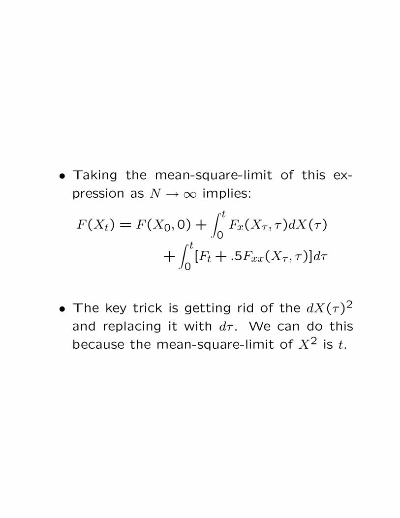
² Taking the mean-square-limit of this ex-
pression as N !1 implies:
F (Xt) = F (X0;0) +Z t
0Fx(X¿ ; ¿)dX(¿)
+Z t
0[Ft + :5Fxx(X¿ ; ¿)]d¿
² The key trick is getting rid of the dX(¿)2
and replacing it with d¿ . We can do this
because the mean-square-limit of X2 is t.
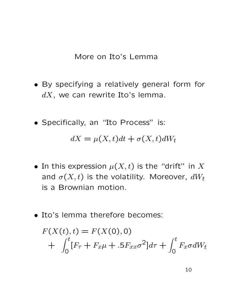
More on Ito's Lemma
² By specifying a relatively general form for
dX, we can rewrite Ito's lemma.
² Speci¯cally, an \Ito Process" is:
dX = ¹(X; t)dt+ ¾(X; t)dWt
² In this expression ¹(X; t) is the \drift" in X
and ¾(X; t) is the volatility. Moreover, dWt
is a Brownian motion.
² Ito's lemma therefore becomes:
F (X(t); t) = F (X(0);0)
+Z t
0[F¿ + Fx¹+ :5Fxx¾
2]d¿ +Z t
0Fx¾dWt
10

² We will see the term F¿ + Fx¹ + :5Fxx¾2
repeatedly.
² Ito's lemma is more usually seen in a stochas-
tic di®erential equation form rather than its
stochastic integral equation form:
dF = FxdX + Ftdt+ :5Fxx¾2dt
dF = [F¿ + Fx¹+ :5Fxx¾2]dt+ Fx¾dWt

Multi-dimensional Ito's Lemma
² If we have a function of multipe stochastic
variables xi, i = 1; : : : ; N, there is a multi-
dimensional version of the Ito equation:
dF = [Ft +NX
i=1
¹iFi + :5NX
i=1
NX
j=1
Fij¾ij]dt
+NX
i=1
Fi¾idWi
where ¾ij = E(dWidWj).
11

Contingent Claims Pricing:
Arbitrage Derivation a la Black-Scholes
² If we make certain assumptions about the
stochastic process that an underlying claim
follows can use the stochastic calculus tools
to determine the value of a contingent claim
on this underlying (such as a forward or an
option).
² In particular, if the underlying follows an
Ito Process, we can show that the contin-
gent claim's value solves a particular partial
di®erential equation. This can be shown in
two ways, both of which center on the con-
cept of arbitrage.
12

² We will derive this PDE both ways. For
simplicity, we will assume the underlying
asset price follows a so-called \geometric
Brownian Motion" (GBM):
dSt = ¹Stdt+ ¾StdWt
where St is the underlying price at t, and
¹ and ¾ are constants. This is called a
\stochastic di®erential equation" (SDE).
² In a GBM, the asset price can never be-
come negative, and percentage changes in
the asset price (returns) are normally dis-
tributed.

Key Assumptions
² We will make some key assumptions in our
analysis. Speci¯cally:
² Zero taxes.
² Zero transactions costs.
² Continuous trading. That is, markets are
always open and you can trade every in-
stant of time without impacting price.
² Constant risk free interest rate (we will
loosen this assumption later.)
13

Deriving the Valuation PDE
² Consider any contingent claim on S. This
could be a futures, a forward, an option,
or something more exotic.
² Posit that the value of the contingent claim
is a function V (St; t).
² Form a portfolio consisting of ¢ units of
the underlying and one unit of the contin-
gent claim. The value of this portfolio is
¦ ´ St¢ + V (St; t).
² By Ito's lemma, the dynamics of this claim
are:
¢dSt + VsdSt + Vtdt+ :5VssdS2t
14

² Substituting from the SDE for dSt,
d¦ = (¹St¢ + ¹StVs + Vt)dt
+ ¾St(¢ + Vs)dWt + :5¾2S2t dt
² Note that the last term comes from the
fact that dW2t = dt.
² We can make this portfolio riskless by set-
ting ¢ = ¡Vs. Our equation then be-
comes:
d¦ = Vtdt+ :5¾2S2t Vssdt
² Since this portfolio is riskless it must earn
the risk free interest rate. That is, d¦ =
r¦dt = rSt¢dt + rV (St; t)dt = ¡rStVsdt +
rV dt.

² This implies:
¡rStVsdt+ rV dt = Vtdt+ :5¾2VSSS2t dt
² This is a second order parabolic PDE.
² This implies our valuation equation:
rV = Vt + rStVs + :5¾2S2t Vss
² Note that this equation holds for any claim
on S.

Boundary Conditions
² The only thing that di®erentiates distinct
contingent claims on the same underlying
(e.g., on the same stock) is their boundary
conditions.
² For instance, for a call expiring at T with
strike price X, we know that V (ST ; T ) =
max[ST ¡ X;0]. For a put, we know that
V (ST ; T ) = max[X ¡ ST ;0]. For a forward
contract, we know that V (ST ; T) = ST .
² These payo® conditions are not su±cient
to determine V . We need two additional
boundary conditions. These are also driven
by the nature of the problem. For instance,
with a European call we know that V (0; t) =
0 and limS!1 = S ¡ e¡r(T¡t)X.
15

² Other examples. For an American call we
know that a smooth pasting condition must
hold. For knock-out option (say a knock-
out call) the value of the claim has to be
zero at the barrier.
² Given the PDE and the barrier conditions,
we can solve for the value of the claim.

A Remarkable Feature
² Note that the value of the contingent claim
does not depend on the \true" drift of S.
That is, ¹ does not appear in the PDE.
The true drift is the expected return, and
depends on the risk aversion (i.e., the pref-
erences) of investors.
² For this reason, this is sometimes called
\preference free" pricing.
² Instead of the true drift, the risk free in-
terest rate appears in the valuation PDE.
16

² That is, you can value the contingent claim
as if the expected return on the undelrying
equals the risk free rate. This would be
true in general if and only if all investors are
risk neutral. That is why this is sometimes
referred to as \risk neutral" pricing.
² This result is an artifact of hedging. Due to
continuous trading and the absence of ar-
bitrage, an investor can hedge away all risk
of holding the contingent claim by trading
the underlying.
² The hedge must be adjusted dynamically
and continuously because Vs changes with
the underlying price.
² Contingent claims are valued by replication
(i.e., hedging) not by expectation. The
drift a®ects expected payo®s, but this does
not matter for valuation purposes.

² Thus, if the underlying is traded, we can
pretend that we are in a risk neutral world.
² This is a wonderful feature because it is
notoriously hard to estimate the true drift
of asset prices.
² The alternative derivation of the pricing
equation arrives at the same conclusion us-
ing a di®erent mathematical approach.

A Convenient Change in Variables
² The foregoing PDE is somewhat cumber-
some because it has non-constant coe±-
cients (that is, the coe±cients depend on
St). Consider the following change of vari-
ables Zt = ln(St).
² By Ito's lemma,
dZ = (¹¡ :5¾2)dt+ ¾dWt
² Using this change in variables
rV = Vt + (r ¡ :5¾2)Vz + :5¾2Vzz
² Note that this equation has constant co-
e±cients if ¾ is a constant. This makes
numerical solution easier.
17

What Happens When the Underlying is Not
Traded?
² The foregoing analysis depends on the as-
sumption that the investor can hedge away
the dWt risk by trading the underlying{there
is a nice linear relationship between dSt and
dWt. What if the underlying itself is not
traded?
² This is relevant in many contexts. For in-
stance, if the underlying risk factor is an
interest rate, the interest rate itself is not
traded. As another example (that we will
explore in more detail later), if volatility ¾ is
not a constant or a function of St, but is in-
stead a stochastic process, then an option
price is a function of a non-traded asset{
the volatility.
18

² Other examples: weather derivatives and
power derivatives. Weather is obviously
not a traded asset, but there are deriva-
tives written on weather. Similarly, since
power is not storable, you cannot create a
hedge portfolio that involves holding a po-
sition in spot power{I must consume power
the instant I purchase it, and cannot re-sell
it even an instant later.
² We can use our hedge derivation even if
the underlying isn't traded, but we will no
longer be able to derive preference free re-
sults. Instead, our pricing equations will
depend on the true drift. Equivalently, any
pricing equation will have a \market price
of risk."

Pricing with a Non-Traded Underlying
² Consider two contingent claims on some
non-traded underlying x. The claim with
value denoted by V expires at time T . The
claim denoted by G expires at time T 0 > T .
² The SDE for x is:
dxt = Ádt+ ¾xdZt
where Zt is a Brownian motion. and ¾x and
Á are functions of x and t.
² Form a portfolio consisting of one unit of
V and ¢ units of G. By Ito's lemma, the
dynamics of this portfolio are:
d¦ = (¢ÁGx + ÁVx + Vt + ¢Gt + :5¢¾2xG
2xx
+ :5¾2xV
2xx)dt+ ¾x(Vx + ¢Gx)dZt
19

² Choose ¢ to make the portfolio riskless.
This requires ¢ = ¡Vx=Gx.
² Since the portfolio is riskless, and requires
initial investment V ¡¢G,
rV ¡r¢G = Vt+¢Gt+:5¢¾2xG
2xx+:5¾2
xV2xx
² Collecting all V terms on the lhs and all G
terms on the rhs:
rV ¡ Vt ¡ :5¾2xVxx
Vx=rG¡Gt ¡ :5¾2
xGxx
Gx

² Note that we only have one equation but
two unknowns (V and G). Note, however,
that the lhs is a function of T (and not
T 0) whereas the reverse is true of the rhs.
This is possible if and only if both sides are
independent of the maturity date. Thus,
there exists some function a(x; t) such that
rV ¡ Vt ¡ :5¾2xVxx
Vx= a(x; t)
² This is conventionally rewritten:
a(x; t) = Á¡ ¾x¸(x; t)
² The function ¸ is referred to as the \mar-
ket price of x risk."

² Using this de¯nition, we derive the follow-
ing PDE:
rV = Vt + :5¾2xVxx + (Á¡ ¾x¸)Vx

² Note that this equation depends on the
true drift of the x process{we can't em-
ploy the convenient assumption that the
drift of the underlying process is equal to
the risk free rate.
² Note that this derivation is more general
than the earlier one because it implies the
basic valuation equation for a traded asset.
Note that a traded asset itself must satisfy
the PDE. Thus:
rS = (Á¡ ¾x¸)
² When Á = ¹S and ¾x = ¾S, this implies:
¸ =¹¡ r¾
² Plugging this for ¸ in the PDE involving
(Á ¡ ¾x¸) returns the basic valuation for-
mula derived earlier. Note that we cannot
use this trick unless x is a traded asset.

Solving PDEs Using Finite Di®erence
Methods
² Solution of a PDE requires determination
of a function that satis¯es the relevant equa-
tion at every possible value.
² Most PDEs have no closed form solution.
Even the heat equation and Black-Scholes-
Merton equations require numerical approx-
imation.
² More complicated numerical approximation
schemes are required to solve PDEs with
boundary conditions that are more compli-
cated that BSM.
² Finite di®erence methods are the most com-
mon means to solve PDEs.
20

The Crank-Nicolson Approach
² There are two basic ¯nite di®erence schemes{
explicit and implicit. The binomial model
is an example of an explicit scheme.
² Explicit schemes are simpler, but (a) can
face stability problems, and (b) don't con-
verge as quickly.
² Implicit schemes are generally superior, but
a method that combines implicit and ex-
plicit methods{the Crank-Nicolson routine{
has very desirable convergence and stability
properties.
21

Implementing Crank-Nicolson
² All ¯nite di®erence schemes start with a
grid. That is, the state variables and time
variable are discretized.
² Consider a stock price model in which the
natural log of the stock price Z is used
as the state variable. Assuming constant
¾ and r, we know that the value of any
contingent claim on this stock must satisfy
the following PDE:
@V
@t+ (r ¡ :5¾2)
@V
@Z+ :5¾2@
2V
@Z2= rV
² Solution of the PDE via ¯nite di®erences
requires approximation of the relevant par-
tial derivatives on the grid.
22

² Step 1: Create a grid. There are I log
stock price points i = 1; : : : I. Although
it is not necessary, assume that the grid
points are evenly spaced, with each one ±Z
apart. There are K time steps. Each step
is ±t in length. The notation is that time
step k = 0 at expiration, and today is k =
K±. This notation is used because solution
involves moving backwards through time in
the grid, going from values we know (at
expiration) to those we don't.
² Step 2: Estimate the partial derivatives.
Di®erent schemes use di®erent estimates.
In Crank-Nicolson, at node i; k of the grid:
@V
@Z¼ :5[
V k+1i+1 ¡ V
k+1i¡1
2±Z
+V ki+1 ¡ V ki¡1
2±Z]

where i indicates the stock price step and k
indicates the time step, and V ki is the value
of the contingent claim at node i; k.
@2V
@Z2¼ :5
V k+1i+1 ¡ 2V k+1
i + V k+1i¡1
(±Z)2
+:5V ki+1 ¡ 2V ki + V ki¡1
(±Z)2
@V
@t¼ V ki ¡ V
k+1i
±t
² Using this approximation, the valuation PDE
can be rewritten as:
¡AV k+1i¡1 + (1¡B)V k+1
i ¡CV k+1i+1 =
AV ki¡1 + (1 +B)V ki +CV ki+1
where A = ¡ ±t4±Z(r ¡ :5¾2) + ±t
4±Z2¾2, B =
¡ ±t2±Z2¾
2 + :5r±t, and C = ±t4±Z(r ¡ :5¾2) +
±t4±Z2¾
2.

² In matrix form, we observe:
MLvk+1 =MRvk
where
ML =
0BBBBBB@
¡A (1¡B) ¡C 0 : : :0 ¡A (1¡B) : : : :: 0 : : : 0 :: : : : 1¡B ¡C 0: : : 0 ¡A (1¡B) ¡C
1CCCCCCA
vk+1 =
0BBBBBBBBBBBBBBBB@
V k+10
V k+11:::::
V k+1I¡1
V k+1I
1CCCCCCCCCCCCCCCCA

MR =
0BBBBBB@
A (1 +B) C 0 : : :0 A (1 +B) : : : :: 0 : : : 0 :: : : : 1 +B C 0: : : 0 A (1 +B) C
1CCCCCCA

and
vk =
0BBBBBBBBBBBBBBBB@
V k0V k1:::::
V kI¡1
V kI
1CCCCCCCCCCCCCCCCA

Solving The Equation System
² The above shows that the solution of the
PDE involves the solution of a set of linear
equations.
² Unfortunately, as written, we have I ¡ 1
equations (the I ¡ 1 rows of the matrices)
in I + 1 unknowns. We need additional
equations. These come from the boundary
conditions. These give us the value of V
at the top and the bottom of the grid.
² Boundary conditions are de¯ned by the prob-
lem. For a European put struck at X,
for instance, we know that when S = 0,
the put value is Xe¡r(T¡t). Thus, V k+10 =
Xe¡r(k+1)±t. Similarly, when S is very large,
the value of the put is zero. Thus, V kI = 0.
23

² We can now rewrite our equation systems
as:
MLvk+1 + rk =MRvk
where
ML =
0BBBBBB@
(1¡B) ¡C 0 : : :¡A (1¡B) : : : :0 : : : 0 :: : : : 1¡B ¡C: : : 0 ¡A (1¡B)
1CCCCCCA
vk+1 =
0BBBBBBBBBBB@
V k+11:::::
V k+1I¡1
1CCCCCCCCCCCA

vk =
0BBBBBBBBBBB@
V k1:::::
V kI¡1
1CCCCCCCCCCCA
rk =
0BBBBBBBBBBB@
¡AV k+10
00::0
¡CV k+1I
1CCCCCCCCCCCA

Solving the PDE
² The essence of the solution technique should
now be easy to understand.
² Start with what you know{the payo® to the
option at expiration. For a put with strike
price X, for instance, at expiration V 0i =
max[SeZ0i ¡ X;0], where S is the current
stock price.
² Given V 0i , 8i, you know v0. Then you can
solve the linear equation system for v1.
² Now you know v1, you can solve for v2.
Continue this process until you get to vK.
24

Solving the linear equation system:
The LU Decomposition
² We want to solve the following equation
for vk+1:
MLvk+1 =MRvk ¡ rk
² The brute force way to solve this equation
is to invert ML. This is computationally
expensive.
² There are other solution techniques that
are much more e±cient computationally.
² For European options, the LU decomposi-
tion is the best approach.
25

² You can decompose the square matrix MLinto
two other matrices, one of which has non-
zero elements only on the diagonal and the
sub-diagonal (L) and another which has
non-zero elements only on the diagonal and
the superdiagonal (U) such that ML = LU.
Also, you can scale things so that L has
ones on the diagonal.
² To apply the LU decomposition, de¯ne q =
MRvk ¡ rk.
² Then LUv = q: One can exploit the sparse-
ness of L and U to solve this equation for
v.
² This is computationally more e±cient be-
cause due to the diagonality of L and U,
they can be inverted using back-substitution.

This involves sequential solution of N equa-tions (where N is the number of rows andcolumns in the matrix of interest), eachwith a single unknown.
² Matlab (and some other programs) use LUdecomposition to invert matrices. There-fore, if you are using Matlab (or one ofthese other programs) you don't need todo the decomposition yourself. Just useinv(ML) or ML
¡1.
² So far we have assumed that ¾ and r don'tvary over time. In this case, you only haveto calculate [LU]¡1 once, and apply it ateach time step.
² In more complicated problems, ¾ and r maydepend on time and the state variable. Inthis case, A, B, and C will depend on k andi, and the LU decomposition and inverstionmust be done at each time step.

Solving the linear equation system:
The SOR Method
² The LU method is quick (especially with
time and state independent coe±cients),
but is not readily applicable to American
options. The Successive Over-Relaxation
(SOR) method is somewhat slower, but
can handle American option problems.
² SOR solves for vk+1 iteratively. For Euro-
pean options the procedure is as follows.
First, one chooses an \over-relaxation pa-
rameter" !; 1 · ! · 2. For n = 1, choose
! = 1. Then de¯ne matrices D, L, and
U so that ML = D + L + U. De¯ne M! =
D +!L and N! = (1¡!)D¡!U. Given an
initial guess of vk+1n , solve:
vk+1n+1 = M!
¡1N!vk+1n + !M!
¡1q
26

² In this expression n is the iteration number.
² Note that you can solve for the entire vec-
tor of v for a given time step with one set
of matrix operations.
² Usually the initial guess vk+10 is the option
value at the previous time-step.
² Continue to iterate until you achieve con-
vergence (within some user-speci¯ed error
tolerance). Convergence means that the
change in v from iteration n to iteration
n+ 1 is small. Formally, calculate:
IX
i=1
(vn+1i ¡ vni )2
and stop when this sum gets su±ciently
small.

² Proceed to the next time step.
² Always keep track of the number of iter-
ations until convergence. After ¯nishing
one time step, increase ! by a little bit
(say .05). If the number of iterations re-
quired for convergence for that time step is
smaller than for the previous step, increase
! a little more for the next time step. If
the number of iterations increases, use the
! from the previous time step for the re-
mainder of your analysis.

² For American options, at each iteration
step, you can't use a matrix operation be-
cause it is necessary to take into account
the possibility of early exercise.
² With an American option, at a given time
step k for each stock price step i (starting
with i = 2) calculate:
vn+1ik = vnik+
!
Mii(qi¡
i¡1X
j=2
Mijvn+1kj ¡
I¡1X
j=i+1
Mijvnkj)
² In this expression Mij is the element in row
i and column j of the ML matrix and qi is
the element in row i of the q vector.

² Note that in this method, to solve for the
option value at stock price node i you use
the option values for nodes 1;2; : : : ; i ¡ 1.
Immediately after solving for the value of
vn+1ik using this method, compare this to
the exercise value of the option. If the
exercise value of the option exceeds vn+1ik ,
replace vn+1ik with the option exercise value
for use in calcuating vn+1(i+1)k
. If the exercise
value is smaller, use the vn+1ik calcuated us-
ing the above formula.

Improving Accuracy:
Richardson Extrapolation
² The greater the number of time steps and
asset steps, the more accurate your solu-
tion. The Crank-Nicolson method is accu-
rate O(±t2; ±Z2).
² Increasing accuracy in this way is compu-
tationally expensive, because the number
of calculations is proportional to 1=±t±Z.
² Richardson extrapolation allows you to get
accuracy O(±t2; ±S3).
27

² To implement RE, ¯rst solve the problem
for a given number of asset steps (e.g.,
20). Call the value of the option given this
approach V1 and the asset step ±S1. Then
increase the number of asset steps (e.g., to
30). Call the option value using this grid
V2 and the asset step ±S2. The RE value
of the option is:
V ¤ =±S2
2V1 ¡ ±S21V2
±S22 ¡ ±S2
1

Jump Conditions
² Handling discrete cash °ows (e.g., dividends)
and some other conditions (e.g., periodic
rather than continuous monitoring of a bar-
rier for a barrier option) requires use of so-
called \Jump Conditions." They are called
this because key variables (e.g., the stock
price) jumps when something happens (e.g.,
a dividend is paid.
² Assume a dividend of size D will be paid at
time td. Note that the value of the option
must not change as a result of the dividend
payment (everyone knows the dividend will
be paid). Immediately before the dividend
is paid, the option is worth V (S; t¡d ). Imme-
diately afterwards, it is worth V (S¡D; t+d ).
Thus, V (S; t¡d ) = V (S ¡D; t+d ).
28

² We address this problem as follows. Pro-
ceed backwards through the grid in the
usual fashion. When you reach td, solve the
value of the option in the usual way. Then
implement the jump condition. At each as-
set step i at time step k (corresponding to
td), de¯ne Zi = ln[exp(Zi)¡D].
² Next de¯ne:
i¤ = Int[Zi ¡ Z0
±Z
¹ =Zi¤+1 ¡ Z
±Z
V (Zi; t¡d ) = ¹V (Zi¤; t
+d )+(1¡¹)V (Zi¤+1; t
+d )
² You have to be careful when i is small, as
in this case i < 0. In this case, just use
i¤ = 0 and ¹ = 1.

² You have to be clever about setting up your
time steps. In certain cases, you can just
move the dividend to the closest payment
date (taking care to adjust by the time
value of money involved in displacing the
timing of the dividend). Alternatively, you
can create a new time step corresponding
exactly to the divident payment. Here you
have to be careful when constructing your
±t to make sure that at that new time step
you are using the right ±t when calcuating
your A, B, and C coe±cients.
² If the option is an American call, you have
to take into account the possibility of early
exercise. In this case, you need to utilize
the SOR technique discussed earlier.

Martingale Methods
² There is an alternative (and equivalent)
way to value derivatives. This involves use
of Martingale Methods.
² In essence, Martingale Methods imply that
any derivative can be valued by calculating
its discounted expected cash °ows under
some probability measure.
² Calculating an expectation involves inte-
grating over the relevant probability mea-
sure.
² Thus, integration methods (Gaussian, Monte
Carlo) can be used to value derivatives.
29

² Some elegant mathematical theory{notably
Kolmogorov's backward equation and the
Feynman-Kac formula{show that the value
function implied by calculating the expec-
tation under the relevant probability mea-
sure must satisfy the same valuation PDE
we derived using the Black-Scholes arbi-
trage approach. Thus, the two methods
are di®erent ways of skinning the same cat
(apologies to PETA members).
² The fact that the methods are equivalent
derives from the fact that the absence of
arbitrage is a necessary (and sometimes
su±cient) condition for the existence of
the relevant probability measure required
to calculate the expectation.

Martingales
² A martingale is a \zero drift" stochastic
process. That is, Wt is a martingale if
E[WT jWt] = Wt 8T ¸ t
² Martingales have very desirable properties
that facilitate solution of valuation prob-
lems.
30

Probability Measure
² A probability measure assigns probabilities
to events.
² Formally, de¯ne a state space that de-
¯nes all the possible states of the world{all
the things that can happen. An event is a
group of states of the world.
² A ¾-¯eld allows speci¯cation of sets of events
to which probabilities can be assigned. A
¾-¯eld A on has the following properties
(a) 2 A, (b) if Ai 2 A, then the comple-
ment of Ai, ACi 2 A, and (c)if Ai 2 A; i =
1; : : : ; n then [ni=1Ai 2 A.
31

² The elements of A are called measurable
sets. A probability measure associates to
each measurable set a real number in [0;1].
The probability measure P has several prop-
erties: (a) P() = 1; (b) if Ai \ Aj =
; 8i 6= j, then P([ni=1Ai) =Pni=1P(Ai);
and (c) P(;) = 0.
² A probability measure quanti¯es the likeli-
hood of events. A triplet f;A;Pg is called
a proability space.

² In ¯nancial mathematics and engineering
the probability measure is almost always
the Gaussian (or normal) distribution. The
Gaussian distribution is like the streetlight
under which the drunk looks for his keys{
we use it not necessarily because it is ap-
propriate, but because the light is better
there.

Equivalent Measures
² The concept of an equivalent measure is
key in modern valuation theory.
² Consider a probability measure P that de-
¯nes the probability that a particular ran-
dom variable Z will take a particular value.
An equivalent measure Q (a) has same null
sets, but (b) a di®erent mean. That is, if
P(Z = Z¤) = 0, then Q(Z = Z¤) = 0, but
EP[Z]6= EQ[Z].
² We care about probability measures for stochas-
tic processes. Consider a stochastic pro-
cess Xt with associated probability mea-
sure P. To be speci¯c, assume dXt =
°(X; t)dt + ¾(X; t)dWt. dWt is a Brownian
motion under the probability measure P.
32

² De¯ne processes u(X; t) and ®(X; t) such
that
¾(X; t)u(X; t) = °(X; t)¡ ®(X; t)
Assume E[expf:5 R t0 u(x; s)2dsg] < 1. De-
¯ne a process Mt as follows:
Mt = expf¡Z t
0u(s)dWs ¡ :5
Z t0u(s)2dsg
² Given these preliminaries, we can state an
important result that eases valuation prob-
lems. This is called Girsanov's theorem.

Girsanov's Theorem
² Girsanov's theorem states that if we start
with a process Xt, we can create another
process that has an arbitrary drift ®(X; t)
under an equivalent measure Q. Speci¯-
cally,
dXt = ®(X; t)dt+ ¾(X; t)d ~Wt
where d ~Wt is a Brownian motion under the
probability measure
dQ= MtdPMt is referred to as the Radon-Nikodym
derivative.
² Equivalently,
d ~Wt = u(X; t) + dWt
33

² In essence, Girsanov's theorem states that
given an initial process, we can create an
equivalent process with an arbitrary mean
by adjusting simultaneously the probability
measure. This adjusted probability mea-
sure is called an equivalent measure.
² Note that ~Wt is a martingale under the al-
ternative measure Q, but not under the
original measure P. Similarly, Wt is a mar-
tingale under P, but not under Q.
² There are arbitrarily many equivalent mea-
sures. One special equivalent measure is an
equivalent martingale measure. Under an
equivalent martingale measure, discounted
prices of securities are martingales. That
is, for an asset price S, if interest rates are
constant, under the equivalent martingale
measure Q,
EQ[e¡r(T¡t)ST jSt] = St

If interest rates are stochastic,
EQ[e¡R Tt r(s)dsST jSt] = St

The Link Between the Absence of Aribtrage
and the
Existence of an Equivalent Martingale
Measure
² Girsanov's theorem is extremely useful be-
cause there is a link between the absence
of arbitrage and the existence of an equiv-
alent martingale measure. There are two
key results.
² First, if there exists an \equivalent martin-
gale measure" Q such that all discounted
prices processes are martingales under Q,
then there are no arbitrage opportunities.
² Second, under certain technical conditions,
the absence of arbitrage implies the ex-
istence of a unique equivalent martingale
measure.
34

² In ¯nite state space models, the absence of
arbitrage always implies the existence of an
equivalent measure. In continuous models
(with an in¯nite number of states), addi-
tional technical conditions are required to
ensure the existence of an equivalent mea-
sure.
² This is where Girsanov's theorem comes
in. The theorem tells us how to create an
equivalent measure so that asset prices rise
at the risk free rate.
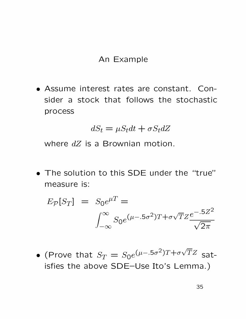
An Example
² Assume interest rates are constant. Con-
sider a stock that follows the stochastic
process
dSt = ¹Stdt+ ¾StdZ
where dZ is a Brownian motion.
² The solution to this SDE under the \true"
measure is:
EP[ST ] = S0e¹T =
Z 1¡1
S0e(¹¡:5¾2)T+¾
pTZe
¡:5Z2
p2¼
² (Prove that ST = S0e(¹¡:5¾2)T+¾
pTZ sat-
is¯es the above SDE{Use Ito's Lemma.)
35

² Referring back to the statement of Gir-
sanov's theorem, I can choose an arbitrary
drift by adjusting the probability measure.
² I want a drift rSt. Thus, if I choose:
u(S; t) =¹¡ r¾
and a new Brownian motion:
d~Zt = u(S; t) + dZt
I get:
dSt = rSt + ¾Std~Zt

where ~Zt is a martingale under the equiva-
lent measure Q:
dQ=e¡:5 ~Z2
p2¼

Using the Martingale Approach
² The martingale approach allows us to de-
termine the value of any contingent claim
expiring at T as:
V = EQ[Pt(St)e¡R T
0 r(s)ds]
where Pt(St) is the payo® to the claim at
t · T .
² Once we have established the equivalent
measure, we can value any contingent claim
by calculating an expectation over this mea-
sure.
² Expectations involve calculations of inte-
grals. Thus, implementing the equivalent
martingal approach entails use of numerical
integration. Numerical integration meth-
ods include Gaussian quadrature and Monte
Carlo techniques.
36

Numeraires
² A \numeraire" is an asset used to discountcash °ows.
² So far we have implicitly worked using a
particular \numeraire" to discount cash °ows
in our valuation formulae. This is the \moneymarket account" numeraire. This is an ac-
count that grows at the risk free rate of
interest.
² Although the money market account is the
most common numeraire, it is not the only
one. Moreover, sometimes clever choice of
a di®erent numeraire can make valuation
easier.
² The Numeraire Irrelevance Theorem tells
us that we should get the same value for
a contingent claim regardless of the nu-
meraire we use.
37

² The theorem states that if P and Q are
two numeraires, the value of any contin-
gent claim is given by V :
Vt = PtEP [VT=PT ] = QtEQ[VT=QT ]

² In this expression, the notation EQ (resp.
EP) means that the expectation is taken
under a measure in which VT=QT (resp.
VT=PT ) is a martingale.
² This expression suggests that when we change
numeraires, we must change probability mea-
sures. Girsanov's theorem tells us how to
do this

Determining the Drift Under a Given
Numeraire
² Assume initially that we use the money
market account Bt = ert as the numeraire.
There is another asset, S1t, with dS1t =
¹1S1tdt + ¾1S1tdW1, that we want to use
as a numeraire. Consider the numeraire
ratio Nt = S1t=Bt. By Ito's lemma:
dNt
Nt=dS1t
S1t¡ dBt
Bt¡ dS1t
S1t
dBt
Bt
² Note that dBt=Bt = rdt, and that the last
term in the above expression is therefore
of o(dt). Thus,
dNt
Nt= ¡rdt+ ¹1dt+ ¾1dW1
38

² Now Girsanov's theorem comes into play.
A corollary to the theorem (there are many
ways to express GT) implies that if dWi is
a Brownian motion under the measure im-
plied by the money market numeraire, then
d ~Wi = dWi¡dWi(dNt=Nt) is a Brownian mo-
tion under the measure implied by the new
numeraire.
² Note that dWi¡dWi(dNt=Nt) = ¾1½dt, where
½ = E(dW1dWi).
² We can apply this to the numeraire as-
set. Recall that when the money market
account is the numeraire, dS1t = rS1tdt +
¾1S1tdW1. Thus, when S1t is the numeraire,
dS1t = rS1tdt+ ¾21S1ydt+ ¾1S1td ~W1.
² We can apply this to other assets. Con-
sider asset two, such that when the money

market account is the numeraire dS2t =
rS2tdt + ¾2S2tdW2. Thus, when S1t is the
numeraire, dS2t = rS2tdt + ¾1¾2½S2tdt +
¾2S2td ~W2.

An Example: The Quanto Forward
² A \quanto" is a contract with a payo® de-
termined by an asset with a price expressed
in currency A, but paid in currency B. For
instance, consider a contract with a payo®
equal to the FTSE 100 stock index paid in
dollars. If the index is 4000 at expiration,
the quanto holder gets 4000 dollars.
² It is easy to ¯gure out the value of a for-
ward on the FTSE paid in pounds. As-
suming no dividends for simplicity, using a
pound sterling money market account as
the numeraire, Ft+¿ = eu¿St where u is the
sterling riskless rate and St is the FTSE
spot price.
39

² To price the quanto, let's change numeraires
from the sterling money market to the dol-
lar money market. In doing so, we have to
be careful about converting the sterling to
dollars. Calling Dt the value of the ster-
ling money market at t, and Ct the value
of the dollar/sterling exchange rate, the
dollar value of the old numeraire is DtCt,
where dCt = ¹CCtdt + ¾CCtdWC. Our nu-
meraire ratio Nt is therefore Bt=DtCt. By
Ito's lemma:
dNt
Nt= rdt¡ udt¡ ¹Cdt¡ ¾CdWC + ¾2
Cdt

² Under the old numeraire dSt = uStdt +
¾SStdWS. By GT, under the new measure:
dSt = uStdt¡ ¾C¾S½CSdt+ ¾SStd ~WS
where ~WS is a Brownian motion under the
new measure implied by the new numeraire.
² Call the quanto forward price k. This price
sets the value of the forward contract to
zero. Under the new measure, for a quanto
expiring at T > t
0 = E[(ST ¡ k)=BT ] = e¡r(T¡t)E[ST ¡ k]
² Given the process for S under the new nu-
meraire,
E[ST ] = Ste(u¡½¾C¾S)(T¡t)St
² This implies that k = Ste(u¡½¾C¾S)(T¡t)St.

The Links Between the PDE and Martingale
Approaches:
Komogorov's Backward Equation and
Feynman-Kac
² The martingale and arbitrage approaches
to contingent claim valuation seem extremely
di®erent. In fact, though, they give the ex-
act same answer.
² Two remarkable results prove that these
approaches are equivalent. The ¯rst theorem{
Komogorov's backward equation{is relevant
when interest rates are constant. The second{
the Feynman-Kac formula{is relevant when
interest rates are stochastic.
40

² Kolmogorov's equations states that if one
de¯nes erTu(x; t) = Ex[f(x; T )], where x is
the Ito proces
dx = ¹(x; t)dt+ ¾(x; t)dW
then
ru = ut + ¹(x; t)ux + :5¾2(x; t)uxx
subject to the conditon u(T; x) = f(x).
Under the equivalent measure, ¹(x; t) = r.
This implies:
ru = ut + rux + :5¾2(x; t)uxx
² This is identical to the equation we used
to derive the Black-Scholes formula.
² The Feynman-Kac formula extends this re-
sult to the case of stochastic interest rates.

Another Way of Showing the Equivalence of
the Approaches
² We can also use the Girsanov theorem to
illustrate the equivalence between the ar-
bitrage portfolio and equivalent martingale
approaches.
² Consider an asset with SDE dSt = ¹Stdt+
¾StdWt where dWt is a Brownian motion
under the true probablity measure P.
² We know that under the EMM e¡rtSt is a
martingale. Note:
de¡rtSt = ¡re¡rtSt + e¡rtdSt =
e¡rt[¡rSt + ¹Stdt+ ¾StdWt]
41

² The Girsanov theorem implies we can ¯nd
another process d ~Wt such that
d ~Wt = dWt + dXt
in which ~Wt is a martingale under the prob-
ability measure Q with
dQ= eR t
0XudWu¡:5R t
0X2ududP
² Subsituting, we get:
de¡rtSt = e¡rt[¡rSt + ¹Stdt
+ ¾Std ~Wt ¡ ¾StdXt]

² For this to be a martingale, it must be the
case that the drift is zero. Hence:
St(¡r + ¹+ ¾dXt) = 0
This requires:
dXt =¹¡ r¾
dt
² Now consider a contingent claim V . Its
discounted value must also be a martin-
gale under the equivalent measure. Ito's
lemma implies the dynamics of the dis-
counted value are:
de¡rtV = e¡rt[¡rV + Vt + Vs¹St + :5¾2S2t Vss]dt
+ e¡rt¾StVsdWt
² Next substitute d ~Wt = ¹¡r¾ + dWt. This
implies:
de¡rtV = e¡rt[¡rV + Vt + VsrSt + :5¾2S2t Vss]dt
+ e¡rt¾StVsd ~Wt

² This must be a martingale, which implies:
¡rV + Vt + VsrSt + :5¾2S2t Vss = 0
² Again{the Black-Scholes equation!

Valuing Contingent Claims Through
Integration
² The Martingale approach implies that we
can value contingent claims by taking an
expectation. Taking an expectation involves
integrating over a probability distribution.
² There are two basic integration techniques{
explicit integration, and Monte Carlo inte-
gration.
² Which is appropriate depends on circum-
stances.
42

Explicit Integration
² Let's take the simplest case{a European
call option with time ¿ to expiration struck
at K. The payo® to this option is max[S ¡K;0]. The Martingale approach implies that
the value of this call is:
C(S;K; ¿) =
e ¡r¿Z 1¡1
max[Se(r¡:5¾2)¿¡¾p¿Z ¡K;0]
¢ e¡:5Z2
p2¦
² We note that we can solve for a critical
value of Z, Z¤ such that S ¡K = 0. This
is:
Z¤ =ln SK + (r ¡ :5¾2)¿
¾p¿
43

² Thus
C(S;K; ¿) = e¡r¿Z Z¤
¡1[Se(r¡:5¾2)¿¡¾p¿Z ¡K]
¢ e¡:5Z2dZp
2¦
² Consider the term
Z Z¤
¡1Se¡:5¾
2¿¡¾p¿ e¡:5Z2dZp
2¦
² The exponent is: ¡:5¾2¿¡¾p¿¡ :5Z2. We
can use the trick of \completing the square
to simplify this:
¡:5(¾2¿ + 2¾p¿ + Z2) = ¡:5(Z + ¾
p¿)2
² De¯ne a new variable Y = Z + ¾p¿ . Since
Z · Z¤, Y · Z¤+ ¾p¿ ´ Y ¤ Thus,
Z Z¤
¡1Se¡:5¾
2¿¡¾p¿ e¡:5Z2dZp
2¦=Z Y ¤
¡1Se¡:5Y 2
dYp2¦

² This is SN(Y ¤), where N(:) is the cumu-
lative normal distribution. It can be es-
timated with arbitrary accuracy using nu-
merical techniques.
² Now consider the term
Z Z¤
¡1Ke¡:5Z2
dZp2¦
² This is just KN(Z¤):
² Therefore,
C(S;K; ¿) = SN(Y ¤)¡ e¡r¿KN(Z¤)
² This is the Black-Scholes-Merton formula.

Monte Carlo Integration
² Monte Carlo techniques are extremely com-
mon in ¯nancial applications.
² In a Monte Carlo approach, one simulates
the behavior of the price of the underlying
using large numbers of random draws, and
then calculates the option value as a sam-
ple average of the payo®s of the option.
² Consider an option with 100 days to matu-
rity. First draw 100 standard normal vari-
ables z1; : : : ; z100: This implies a series of
100 stock prices. The stock price on day
j is
Sj = S0e(r¡:5¾2)(j=365)+(¾=
p365)
Pji=1 zi
44

² On day 100, the value of the option is:
max[S100 ¡K;0].
² Save the value of the option at expira-
tion. Repeat this process many times (e.g.,
10,000 times) and take the average of all
the values you get. Discount the average
to re°ect the time value of money. The
discounted average is the value of the op-
tion.

Path Dependent Options
² One advantage of Monte Carlo is that you
can value so-called path-dependent options.
² A path-dependent option has a payo® that
depends on the path the underlying price
follows, not just the value of the underlying
at expiration.
² An example of a path-dependent option
is a \knock-out" call. This option be-
comes valueless if the value of the underly-
ing reaches some level prior to expiration.
² In a Monte Carlo valuation approach, you
can set the value of the option equal to
zero on any path that crosses the \knock-
out" barrier.
45

Increasing the Accuracy of MC
² There are a variety of techniques to im-
prove the accuracy and speed of Monte
Carlo.
² In the antithetic variable technique, in your
¯rst sample use zi, in your second sample
use ¡zi.
46

² The control variable technique requires the
existence of a related option that has an
analytical solution. For instance, consider
an \Asian" option. An Asian option has
a payo® that equals the average of the
underlying price over some time interval.
There is no analytical solution for an Asian
option with a payo® given by an arithmetic
average of prices. There is, however, a an-
alytical solution for the value of an Asian
option based on a geometric average.
² In the control variate technique, calcualate
the value of both the geometric and arith-
metic Asian using MC. Call the value of
the arithmetic option value given by the
MC approximation as A. Call the value of
the geometric value given by the MC as G.
Call the analytical value of the geometric
option G¤. Then estimate the value of the
arithmetic Asian as A+ (G¡G¤).

² Quasi-random sequences use a special al-
gorithm to choose the zi. An example is
the Sobol' sequence. By insuring that there
are fewer \gaps" and \clumps" in the zi,
quasi-random sequences allows you to use
fewer random samples when estimating your
option value. Due to this, the accuracy of
the MC approximation is proportional to
1=M using qrs, instead of 1=pM using a
basic random number generator, where M
is the sample size.

Which Valuation Method is Best?
² Explicit integration is preferable for Euro-
pean options.
² Monte Carlo is frequently the best approach
when (a) valuing options that have payo®s
that depend on several underlying variables
(e.g., stochastic volatility) and (b) certain
path dependent options.
² Monte Carlo cannot handle American op-
tions.
² PDE techniques are best for American op-
tions. Moreover, PDE approaches are fre-
quently °exible enough to value path-dependent
options (such as Asians). This requires
increasing the number of state variables,
which raises computation (and program-
ming) costs.
47

How Well Do These Approaches Work?
² These valuation approaches work well when
its assumptions closely approximate reality.
² The key assumption is that the behavior of
¯nancial prices is well-approximated by an
Ito Process.
² Unfortunately, there's a lot of evidence that
¯nancial prices don't behave like Ito Pro-
cesses.
48
The Volatility Smile
² If volatility is constant, then all options on
the same underlying should have the same
\implied volatility." An implied vol is the
volatility parameter that sets the option
value given by the BSM model equal to
the market price of the option.
² If volatility is a function of S and t, as is
permissable with an Ito Process, then day
after day, the function ¾(S; t) that best ¯ts
options prices shouldn't change.
49

² We know that implied volatility is not the
same for all options. Indeed, there is some-
thing called the volatility smile, or volatility
\smirk." That is, implied volatilities are a
function of the strike price. The implied
vol for at-the-money options is lower than
the implied vol for options with lower strike
prices, and is sometimes lower than the
implied vol for options with higher strike
prices.

Financial Orthodentia:
Fixing the Smile ;-)
² On a given day, you can choose (using
complex mathematical techniques) a func-
tion ¾(S; t) that ¯ts the volatility smile.
² Derman and Kani ¯rst derived a method
for implementing this approach based on
binomial trees. Although this is popular,
and widely used, it is numerically crude.
It faces what as known as an \over¯tting
problem." There is an in¯nite number of
¾(S; t) functions that can ¯t a ¯nite num-
ber of option prices exactly. Which one to
choose? The DK approach always gives
you one such function, but if you change
the data (e.g., the options prices) by the
tiniest amount, the DK approach will give
50

you a completely di®erent function. That
is, the DK approach is not stable.
² There are other, very advanced approaches
that avoid over¯tting. These are called
\inverse techniques."
² Even if you use inverse techniques, you may
run into problems. This technique is good
if and only if the underlying price process
is an Ito process. If it isn't, this approach
will not work.
² There is evidence that stock, bond, and
commodity prices are not Ito processes.

² With an Ito process, using inverse tech-
niques you should get the same ¾(S; t) func-
tion every day. In fact, you don't. More-
over, an Ito process implies that volatility
depends only on the underlying price. In
fact, there is a lot of evidence that volatil-
ity changes a lot and that these changes
cannot be attributed solely to changes in
the underlying price.
² Indeed, there is an immense body of ev-
idence showing that volatility varies ran-
domly over time, and that this variation is
largely independent of movements in the
underlying price.
² Random volatility can explain the smile.
² If volatility is random{that is, stochastic{
then the Ito process-based approach will
give incorrect option valuations.

Valuation With Stochastic Volatility
² Volatility is not a traded asset. Therefore,
if we want to use volatility as a state vari-
able then (a) we now have two state vari-
ables (the underlying and the volatility) and
(b) we have to use a formula with a market
price of risk.
² Let's specify a fairly general S volatility
process:
d¾ = ¹¾ + ºdW¾
where the parameters ¹¾ and º are poten-
tially functions of ¾ and t.
² Then, calling ¸ the market price of volatil-
ity risk, our valuation PDE for a contingent
claim with value V becomes:
51
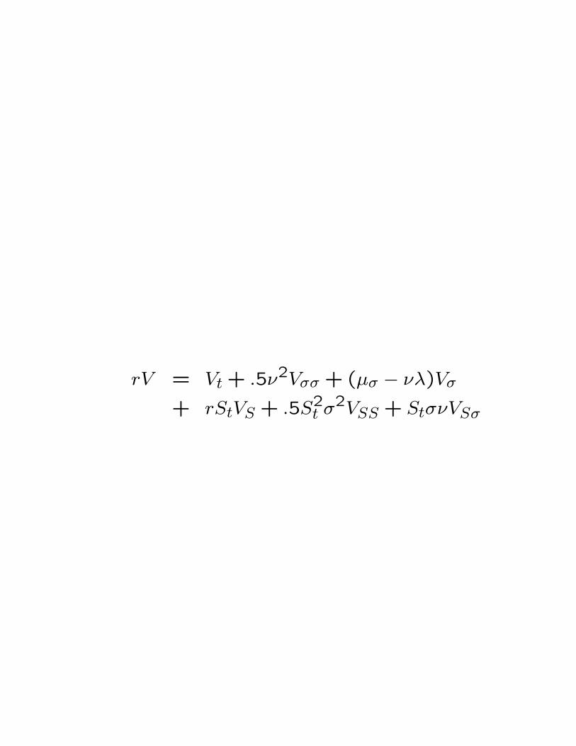
rV = Vt + :5º2V¾¾ + (¹¾ ¡ º¸)V¾
+ rStVS + :5S2t ¾
2VSS + St¾ºVS¾

Implementation
² This is a two-dimensional parobolic PDE.
It can be solve using a variety of meth-
ods, including ¯nite di®erences (especially
useful for American options), Monte Carlo
integration, or Fourier techniques.
52

² Solving the model also requires speci¯ca-
tion of the volatlity process parameters.
There are several standard processes that
are tractible (but perhaps not completely
realistic) used for this purpose.
² Solving the model also requires knowledge
of the current value of ¾ and estimation
of the volatility process parameters. Since
¾ is not observed directly, these are hard
problems. That is, ¾ is a \latent" process
that requires some fancy statistics to es-
timate. One approach is to use discrete
time (e.g., daily data) to estimate the pa-
rameters. This is feasible if the discrete
time model (e.g., a GARCH model) has a
continuous time limit.

² Another problem is that it is necessary to
estimate a market price of risk.
² Initially, practitioners assumed ¸ = 0. Much
empirical evidence shows that this is incor-
rect. If it were true, delta hedged options
positions would earn the riskless rate. In
fact, returns on such positions deviate sub-
stantially from the riskless rate. This im-
plies that there is another risk premium af-
fecting options prices. A likely candidate is
volatility risk.
² ¸ is also an unobserved function.
² The theoretically purest way to address all
these problems is to use historical options
price data as well as underlying price data
to estimate ¹¾, º, and ¸, and these parame-
ters plus current options prices to estimate
¾. This is a demanding process.

Jumps
² Eyeballing any ¯nancial time series one sees
instances where prices seem to change dis-
continuously. That is, they \jump" or \gap."
² Remember that Brownian motions have con-
tinuous sample paths{they do not exhibit
jumps. Thus, Ito processes cannot capture
the jumpiness observed in prices.
² One way to address this issue is to utilize
so-called \jump-di®usion" models. These
marry a Brownian motion process and a
Poisson process.
53

² A Poisson process is one that exhibits no
change with probability 1¡¸dt and changes
with probability ¸dt. That is, the poisson
process q is dq = 0 with probability 1¡ ¸dtand dq = 1 with probability ¸dt. ¸ is re-
ferred to as the intensity of the jump pro-
cess.
² a stock price model that incorporates the
jump is:
dS = ¹Sdt+ ¾SdW + (J ¡ 1)Sdq
² In this expression, J gives the magnitude
of the jump. J can be deterministic (e.g.,
J = :9, indicating that the stock prices falls
10 percent during a jump) or J can be a
random variable.

² Although the jump process can be speci¯ed
quite generally to describe observed data
accurately, jumps pose acute problems for
valuation.
² Remember that the valuation methods that
we have used so far rely on hedging and
replication arguments. The jump compo-
nent cannot be hedged using the underly-
ing, however.
² If the magnitude of the jump is known and
takes a single value (i.e, J is a constant)
then we can construct a hedge portfolio
consisting of two options and the under-
lying. This introduces a market price of
risk.

² If the jump magnitude is stochastic things
get even more complicated. If J takes on K
values, we need a portfolio of K+1 options
and the underlying to hedge all relevant
risks. This injects K risk prices. Note that
if J is a continuous random variable, and
hence K =1, we have an in¯nite number
of risk prices!
² Various models have been proposed to ¯-
nesse this issue. Most implicitly or explic-
itly assume that the jump risk is diversi-
¯able, or can be priced using the CAPM.
Such models calculate values through in-
tegration. These approaches are further
examples of looking for our keys under the
lamppost.
² Jump models also pose serious estimation
issues. That is, it is not a trivial task to
estimate the parameters of a jump process.

² Jump models have become especially pop-
ular for pricing electricity derivatives be-
cause electricity prices are very jumpy. This
points out a serious issue{descriptively ac-
curate characterizations of price processes
may not lead to reliable pricing models.
Even if we know the probability and in-
tensity of jumps, unless we know how the
market prices these jumps we cannot de-
rive reliable pricing models. Even if we can
take expectations under the true measure
(because we have characterized the statis-
tical properties of the jumpy price series)
we can't value unless we know the relevant
probabilities under the equivalent measure.

² Jump models also pose problems in elec-
tricity because ¸ is time dependent{a jump
is more likely in the summer than the fall,
for instance. Moreover, the distribution of
J is almost certainly time dependent{big
jumps are more likely in the summer.
² Jump models provide a great illustration of
the dilemmas of derivative pricing; descrip-
tively accurate models seldom can be in-
corporated in the available valuation frame-
work. Practitioners therefore face a trade-
o® between descriptive accuracy and valu-
ation feasibility.

Interest Rate Models
² One of the most important areas of deriva-
tives modeling involves ¯xed income mar-
kets. Modeling derivatives on ¯xed income
products requires modeling interest rates.
² There are two basic \°avors" of interest
rate models: (a) spot rate models, and (b)
Heath-Jarrow-Morton forward rate models.
² The spot rate models are much more tractible.
We will focus on those.
54

Spot Rate Models
² Spot rate models characterize the dynam-
ics of the instantaneous interest rate{the
interest rate at which you can borrow or
lend over the next instant.
² There is in fact no real world analogue to
the instantaneous spot rate{it is merely a
modeling convenience.
² The generic spot rate model is a single fac-
tor model of the type:
drt = µ(r; t)dt+ ¾(r; t)dz
² Di®erent models make di®erent assump-
tions about µ(:; :) and ¾(:; :).
55

² The earliest model is the Vasicek model:
dr = a(b¡ r)dt+ ¾dz
² in the Vasicek model, a > 0, b > 0, and ¾
are constants. This model exhibits \mean
reversion." That is, when r > b, the spot
rate tends to fall; when r < b, the interest
rate tends to rise. Thus, the interest rate
reverts to the long range mean value of b.
² Interest rates can become negative in this
model. This is a potentially serious prob-
lem (especially when dealing in low interest
rate environments).
² The Cox-Ingersoll-Ross (CIR) model:
dr = a(b¡ r)dt+ ¾prdz

² This \square root process" model rules out
negative interest rates. It implies that in-
terest rate volatility rises with interest rates.
² The Ho-Lee model:
dr = µ(t) + ¾dz
² The Hull-White model:
dr = (µ(t)¡ ar)dt+ ¾dz
² This model adds mean reversion to Ho-
Lee.
² Negative interest rates are possible in both
Ho-Lee and Hull-White.

A Generalized Overview to Pricing Interest
Rate Derivatives
² Given a spot rate model, we can use our
standard pricing techniques to value any
¯xed income derivative.
² Call V (r; t) the value of an interest sensitive
contingent claim. Then:
rV = Vt+:5¾(r; t)2Vrr+[µ(r; t)¡¾(r; t)¸(r; t)]Vr
² Note that we have to include a market price
of risk because the spot rate is not a traded
asset.
² The spot rate models discussed earlier are
used largely because they are tractible, and
allow closed-form solutions of this equation
for certain instruments.
56

² In particular, it is possible to solve analyti-
cally for zero coupon bond prices using the
spot rate models discussed above. A zero
coupon bond that matures at T has the
boundary condition V (r; T) = 1.
² For the spot rate models, the zero coupon
bond price PT is of the form
PT (r; t) = A(t; T)e¡B(t;T)r(t)
² In the Vasicek model:
B(t; T) =1¡ e¡a(T¡t)
a
and
A(t; T) = exp[(B(t; T )¡ T + t)(a2b¡ :5¾2)
a2
¡ ¾2B(t; T)2
4a]

² There is also a closed form solution for
a European call or put option on a zerocoupon bond in the Vasicek model.
² In the CIR model:
B(t; T) =2(e°(T¡t) ¡ 1)
(° + a)(e°(T¡t) ¡ 1) + 2°
A(t; T) = [2°e:5(T¡t)(a+°)
(° + a)(e°(T¡t) ¡ 1) + 2°]2ab=¾
2
where ° =qa2 + 2¾2.
² In the Ho-Lee model, B(t; T) = 1 and
lnA(t; T) = lnP(0; T)
P(0; t)¡ (T ¡ t)@P(0; t)
@t
¡ :5¾2t(T ¡ t)2
² In Hull-White:
B(t; T) =1¡ e¡a(T¡t)
a

lnA(t; T ) = lnP(0; T)
P(0; t)¡B(t; T)
@P(0; t)
@t
¡ 1
4a3¾2(e¡aT ¡ e¡at)2(e2at ¡ 1)

Term Structures
² Each spot rate model implies a term struc-
ture of interest rates. The term structure
is a curve that gives the interest rate as a
function of maturity. The T -period inter-
est rate is the yield on a zero coupon bond
with maturity T .
² The Vasicek model allows an upward slop-
ing, downward sloping, or \humped" term
structure. This is somewhat limiting.
² The Ho-Lee and Hull-White models allow
\exact" ¯tting of the term structure be-
cause of the \fudge factor" µ(t). One can
choose µ(t) to ¯t term structures exactly.
57

² Note that since you are ¯tting the models
to market prices, the µ(t) function implic-
itly includes a market price of risk.
² To calculate µ(t) in HL, collect zero prices
for every maturity. Use these prices (or the
prices from Eurodollar futures or FRAs) to
calculate instantaneous forward rates. An
instantaneous forward rate for time t is the
rate that I can lock in today for borrowing
at t for repayment at t+dt. Call the forward
rate for maturity t F(0; t). Then, in HL:
µ(t) = Ft(0; t) + ¾2t
² This is sometimes approximated as µ(t) =
Ft(0; t), The partial derivative is estimated
using ¯nite di®erences.

² In HW, follow the same data collection pro-
cedure, exept use:
µ(t) = Ft(0; t) + aF (0; t) +¾2
2a(1¡ e¡2at)
² This is often approximated as µ(t) = Ft(0; t)+
aF (0; t)

Calibration
² This process of ¯tting µ(t) is called \cali-bration."
² Calibration gives an exact ¯t to the termstructure.
² This exact ¯t seems comforting, but in factis dangerous. ALWAYS BEWARE A PER-FECT FIT. Perfect ¯tting in fact implies\over¯tting."
² The problem here is similar to the problemwith Derman-Kani discussed earlier. If I ¯tµ(t) using one set of data, and then changethe data only slightly, I'll get a completelydi®erent µ(t).
² Inverse problem techniques are more ap-propriate for this analysis.
58

How Well do Short Rate Models Work?
² Short rate models are extremely popular.
They have some serious problems, though.
² For one thing, single factor models are of
dubious validity. Principal components anal-
ysis suggests that there are multiple factors{
at least three, perhaps as many as 10{
driving interest rates. The three strongest
factors appear to be \shift," \twist," and
\hump." Thus, single factor models can't
mimic the dynamics of real world interest
rates.
² Multi-factor models seem to be a desirable
alternative, but they are considerably more
complicated to implement.
59

² Relatedly, if the models were correct we
should see the same µ(t) functions day af-
ter day. In fact, we don't. This re°ects the
fact that the calibration papers over serious
limitations in the models' ability to capture
real world interest rate dynamics. In partic-
ular, the models cannot reliably capture the
extreme steepness of the term structure at
the very short-maturity section. The ¯t-
ted µ(t) functions imply that the short end
should \°atten out" but it usually doesn't.
² There is also substantial evidence of stochas-
tic volatility in interest rates. The standard
models don't capture this.
Recommended