Original Research Article:
full paper(2020), «EUREKA: Physics and Engineering»
Number 5
91
Mathematical Sciences
FINITE ELEMENT METHOD FOR HEAT TRANSFER
PHENOMENON ON A CLOSED RECTANGULAR PLATE
Collins O. Akeremale
Department of Mathematical Sciences1
Department of Mathematical Sciences
Federal University Lafia
PMB 146, Nasarawa State, Nigeria
Olusegun A Olaiju
Department of Mathematical Sciences1
Department of Mathematics and Statistics
Federal Polytechnics Ilaro
PMB 50, Ogun State, Nigeria
Yeak Su Hoe
Department of Mathematical Sciences1
1Universiti Teknologi Malaysia
81310, Skudai, Johor Bahru
Abstract
In the diagnosis and control of various thermal systems, the philosophy of heat fluxes, and temperatures are very crucial.
Temperature as an integral property of any thermal system is understood and also, has well-developed measurement approaches.
Though finite difference (FD) had been used to ascertain the distribution of temperature, however, this current article investigates
the impact of finite element method (FEM) on temperature distribution in a square plate geometry to compare with finite differ-
ence approach. Most times, in industries, cold and hot fluids run through rectangular channels, even in many technical types of
equipment. Hence, the distribution of temperature of the plate with different boundary conditions is studied. In this work, let’s
develop a finite element method (code) for the solution of a closed squared aluminum plate in a two-dimensional (2D) mixed
boundary heat transfer problem at different boundary conditions. To analyze the heat conduction problems, let’s solve the two
smooth mixed boundary heat conduction problems using the finite element method and compare the temperature distribution of
the plate obtained using the finite difference to that of the plate obtained using the finite element method. The temperature dis-
tribution of heat conduction in the 2D heated plate using a finite element method was used to justify the effectiveness of the heat
conduction compared with the analytical and finite difference methods.
Keywords: finite element method, steady-state, squared plate, analytical method, closed rectangle.
DOI: 10.21303/2461-4262.2020.001422
1. Introduction
Heat conduction is generally simulated in two major ways, direct heat conduction prob-
lem (DHCP) estimation and inverse heat conduction problem (IHCP). In assessing the temperature
distribution within conductive media, direct heat conduction simulation is commonly used. This is
when the existing boundary conditions, the intensity of the heat source within or thermo-physical
properties of the material body is known [1]. While the reconstruction of unknown heat flux or
temperature on the surface of a body conducting heat based on temperature measurements taken at
interior point or backside points is the solution of IHCP [2].
The measurement of random errors is prone to high sensitivity and as such, IHCPs are ill-
posed mathematically. This results in astronomical disorder or perturbation in the solution. Natu-
rally in solids, the nature of transient heat conduction is such that the perturbation on the surface
penetrates and diminishes toward the interior. On the contrary, the least measurement is magnified
Original Research Article:
full paper
(2020), «EUREKA: Physics and Engineering»
Number 5
92
Mathematical Sciences
at the surface, leading to large oscillation and fluctuation in the estimated surface condition when
the interior point is used as an input inverse problem [2].
Temperature and heat flux of a wall in an inaccessible surface can be determined using the
inverse heat conduction method by measuring the temperature on an accessible boundary. Distur-
bances arise in the predicted heat fluxes as a result of the noise in the measure of the temperature.
To measure the temperature at two locales had been demonstrated to improve the predicted heat
fluxes. Installation of an interior thermocouple can result in material inhomogeneities that change
the heat flow through the wall, and in many applications, to adjust the wall to include an interior
thermocouple can’t be achieved. Sensitivity analysis and numerical experiments have demonstrat-
ed that the computation of the temperature can be improved by the absorbing of the measurement
of heat flux at the accessible boundary. Hence, a numerical method to predict the heat transfer on
an inaccessible boundary without changing the thermal boundary condition is necessary.
To establish a correct and stable estimate of the inverse solution, an appropriate approach
is crucial. A major approach amongst the most efficient approaches is called future time measure-
ments and it was first developed in a least-square sequential procedure denoted by the method of
function specification by Beck [3]. The stability of the inverse problem was highly enhanced by
this method. Many improvements had been proposed on the work or method of Beck [4–6]. Many
authors [2, 7–13] had improved on the solution to IHCP especially with the introduction of future
time measurement concepts.
Recent work [1] had used finite-difference to solve the 2D heat transfer problem and the
result compared to the analytical method. The soundness of the temperature distribution was also
ascertained through the finite difference scheme. However, in this work, let’s intend to use a finite
element for the solution of heat transfer problems and to establish or show the pattern of tempera-
ture distribution using the method of finite element. This research is important because heat trans-
fer is not limited to regular bodies or geometry and it had been established that the finite element
method is the best for irregular geometry.
Let’s establish the effectiveness of temperature distribution in the heat conduction process
in a 2D heated plate using the finite element method compared with the analytical method as re-
ported in [1] where finite-difference was used.
2. 2D Heat Conduction in Transient
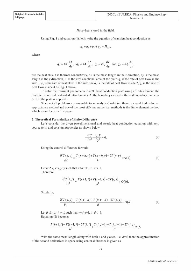
Let’s consider where an explicit method is used, the energy control to a nodal field of the
size is as presented in the Fig. 1 below.
Fig. 1. Transient heat transfer phenomenon using meshes
Hin=0,
Hout=Hin+H. (1)
Hin=heat into the field.
Hg=heat generated in the field.
𝑞𝑞𝑎𝑎 𝑞𝑞𝑐𝑐
𝑞𝑞𝑏𝑏
𝑞𝑞𝑑𝑑
side 3
side 2
side 1
side 4
Original Research Article:
full paper(2020), «EUREKA: Physics and Engineering»
Number 5
93
Mathematical Sciences
Hout=heat stored in the field.
Using Fig. 1 and equation (1), let’s write the equation of transient heat conduction as
,a b c d outq q q q H+ + + =
where
d,
da c
Tq kA
y=
d,
db c
Tq kA
y=
d
dc c
Tq kA
y= and
d
dd c
Tq kA
y=
are the heat flux. k is thermal conductivity, dx is the mesh length in the x direction, dy is the mesh
length in the y direction, Ac is the cross-sectional area of the plate. q
a is the rate of heat flow in the
side 3, qb is the rate of heat flow in the side one q
c is the rate of heat flow inside 2, q
d is the rate of
heat flow inside 4 as Fig. 1 above.
To solve the transient phenomena in a 2D heat conduction plate using a finite element, the
plate is discretized or divided into elements. At the boundary elements, the real boundary tempera-
ture of the plate is applied.
Since not all problems are amenable to an analytical solution, there is a need to develop an
approximate method and one of the most efficient numerical methods is the finite element method
which is our focus in this paper.
3. Theoretical Formulation of Finite Difference
Let’s consider the given two-dimensional and steady heat conduction equation with zero
source term and constant properties as shown below
2 2
2 20.
T T
x y
∂ ∂− − =
∂ ∂ (2)
Using the central difference formula
( ) ( ) ( ) ( ) ( )
2
2 2
, , , 2 ,.
T x y T x h y T x h y T x yO h
x h
∂ + + − −= +
∂ (3)
Let h=Δx, x=i, y=j such that x+h=i+1, x–h=i–1.
Therefore,
( ) ( ) ( ) ( ) ( )2
2 2
, 1, 1, 2 ,.
T i j T i j T i j T i jO h
x h
∂ + + − −= +
∂
Similarly,
( ) ( ) ( ) ( ) ( )
2
2 2
, , , 2 ,.
T x y T x y d T x y d T x yO d
y d
∂ + + − −= +
∂ (4)
Let d=Δy, x=i, y=j, such that y+d=j+1, y–d=j–1.
Equation (2) becomes
( ) ( ) ( ) ( ) ( ) ( )2 2
1, 1, 2 , , 1 , 1 2 ,.
T i j T i j T i j T i j T i j T i jf
h d
+ + − − + + − −+ =
With the same mesh length along with both х and у axes, i. e. h=d, then the approximation
of the second derivatives in space using center-difference is given as
Original Research Article:
full paper
(2020), «EUREKA: Physics and Engineering»
Number 5
94
Mathematical Sciences
( ) ( ) ( ) ( ) ( )1, 1, 4 , , 1 , 1 0.T i j T i j T i j T i j T i j+ + − − + + + − = (5)
After applying the boundary condition, a set of algebraic equations is obtained and solved.
4. Theoretical Formulation of Finite Element
The finite element formulation of the steady-state heat transfer problems using the Galerkin
method with constant properties is given or derived below
2 2
2 20.
T T
x y
∂ ∂− − =
∂ ∂
One of the finite element methods, the Galerkin method differs from other methods in
the way the basis functions are constructed. The domain Ω is portioned into disjoint subdo-
mains called finite elements. For each element Κ, the corresponding shape functions XK which
eventually are glued together into the globally defined basis function Nk in the Galerkin method is
introduced. Galerkin approximation is different from other finite element methods (FEM) through
the construction of the basis functions.
In FEM, the task is to find a linear approximate solution eT s′ over each element which
requires the calculation of unknown T values at each of the nodes of the mesh as shown in the
figure below which will lead to algebraic equations as a result of many values T to be determined.
One of the unique properties of the finite element method in its weak form is that its solution is C0
continuous and includes natural boundary conditions (NBCs) in its formulation.
To convert equation to weak form, let’s multiply both sides of the equation with weight
function say and integrate over the domain of the domain.
Let’s multiply both sides of equation (2) with a test function or wave function say w and in-
tegrate with the condition that the wave function is zero at the boundaries i.e w=0 at the boundaries
( )2. d d .w T A f AΩ Ω
∇ =∫ ∫ (6)
Subject to
. ,n Nu n u→
∇ = Γ and , ,DT T= Γ
where T is the dependent or field variable
Applying Green Theorem
( ). d . d . d 0,w T n T w w f − ∇ Γ − ∇ ∇ Ω − Ω = ∫ ∫ ∫
( ). d . d . d 0.nw u T w w f− Γ + ∇ ∇ Ω − Ω =∫ ∫ ∫ (7)
Now the Discretization by interpolation
Let
,i i
i
w N N= ψ = ψ∑ ,j j
j
T N T NT= =∑ (8)
where Ni is the shape function at each of the nodes and ψ is any constant.
Recall that ( ). d , .a b a bΩ =∫Therefore, ( ) ( ). d , .T w T w∇ ∇ Ω = ∇ ∇∫Let, [ ]0,...1,...0,...,0 .ψ =
Original Research Article:
full paper(2020), «EUREKA: Physics and Engineering»
Number 5
95
Mathematical Sciences
Therefore, ,iw N= ,ini ∈Ω .Ni ∈∂ Where Ω
in belong to internal nodes, ∂
N belong to nodes on
the Newmann boundary condition region.
Substitute (8) into (7)
. d . d . d 0.i i j j i i n i i
i j i i
N N T N u N f
∇ ψ ∇ Ω − ψ Γ − ψ Ω = ∑ ∑ ∑ ∑∫ ∫ ∫ (9)
Let, [ ]0,...1,...0,...,0 ,ψ =
( ), d . d . d 0,i j j i n i
j
N N T N u N f
∇ ∇ Ω − Γ − Ω = ∑∫ ∫ ∫
where i is the row of the matrix, j is the column of linear system
, d . d ( . )d 0,i j j i n i
j
N N T N u N f ∇ ∇ Ω − Γ − Ω = ∑ ∫ ∫ ∫
( ), d . d . d ,i j j i n i
j
N N T N u N f ∇ ∇ Ω = Γ + Ω ∑ ∫ ∫ ∫
where
, ,j j
j
N NN
x y
∂ ∂∇ =
∂ ∂ , ,i i
i
N NN
x y
∂ ∂∇ =
∂ ∂
( ), . , d . d . d ,j j i i
j i n i
j
N N N NT N u N f
x y x y
∂ ∂ ∂ ∂Ω= Γ + Ω ∂ ∂ ∂ ∂
∑ ∫ ∫ ∫ (10)
d .j ji i
ij
N NN NK
x x y yΩ
∂ ∂ ∂ ∂= + Ω ∂ ∂ ∂ ∂
∫ (11)
d .
j
i i
ijj
N
N N xK
Nx y
y
Ω
∂ ∂ ∂ ∂ = Ω
∂ ∂ ∂ ∂
∫ (12)
Recall that from the transformation, ( ) ( )( )( , ) , , , ,= ε ηN x y N x y x y
,x yN N x N yε ε ε= +
,x yN N x N yη η η= +
,x
y
NN x y
x y NN
ε ε ε
η ηη
=
(13)
where
Jacobian ,x y
x y
ε ε
η η
=
,x
y
NNJ
NN
ε
η
=
Original Research Article:
full paper
(2020), «EUREKA: Physics and Engineering»
Number 5
96
Mathematical Sciences
1 .x
y
N NJ
N N
ε−
η
=
Equation (11) becomes
1 1 d .
Ti j
ij i j
N NK J J
N N
ε ε− −
Ω η η
= Ω
∫ (14)
Let
1 ,
i
i i
NB J
N
ε−
η
=
(15)
d ,T
ij i jK B BΩ
= Ω ∫
. d ( . )d .i i n if N u N f= Γ + Ω∫ ∫Equation (9) becomes,
( )d . d . d ,T
j i n i
j
B B T N u N fΩ
Ω = Γ + Ω
∑ ∫ ∫ ∫
[ ][ ] [ ].K T F=
This linear system of equation is then solved for each of the element and the matrices and
their source terms are them assembled to form the system of equation for the whole domain.
5. Numerical Examples
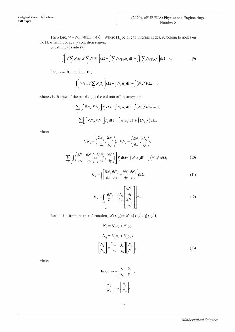
Example 1. Let’s consider a smooth 2D heat conduction plate problem in Fig. 2 below in
which the temperature of the side 3 of the plate is 400sin(πx) °C and it is 0 °C on side 1. The left and
right side temperature of the plate is 0 °C respectively with exact solution given as
( ) ( ) ( )400 400sin .
y y
exact
e eT x
e e e e
π −π
−π π −π π
= − + π
π − π −
The length and width of the plate are 1m as shown in the Fig. 2 below [1]
Fig. 2. 2D rectangular plate with Dirichlet condition
This problem is solved using finite element at different meshes and the temperature dis-
tributions are shown in Fig. 3, 4 below as compared with the finite difference method as shown
in Fig. 10, 11.
𝑦𝑦
𝑥𝑥 0 𝑇𝑇 = 0 °C
𝑇𝑇 = 00𝐶𝐶
𝑇𝑇 = 0 °C
𝑇𝑇 = 400 sin 𝜋𝜋𝑥𝑥 °C
𝐿𝐿 = 1𝑚𝑚
𝐿𝐿 = 1𝑚𝑚
Original Research Article:
full paper(2020), «EUREKA: Physics and Engineering»
Number 5
97
Mathematical Sciences
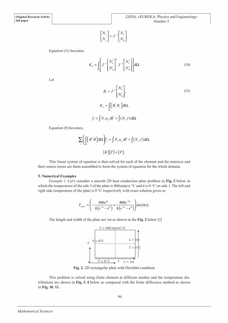
The FE temperature distribution is shown in Fig. 3, 4 as compared with FD temperature
distribution as shown in Fig. 5, 6 below.
Fig. 3. Temperature distribution (h=k=0.1)
Fig. 4. FE temperature distribution for (h=k=0.02)
Fig. 5. Temperature distribution (h=k=0.1)
Fig. 6. FD emperature distribution for (h=k=0.02)
Original Research Article:
full paper
(2020), «EUREKA: Physics and Engineering»
Number 5
98
Mathematical Sciences
Fig. 3, 4 above shows that FEM produced accurate results in predicting the temperature
distribution of a plate on a regular grid used in this work.
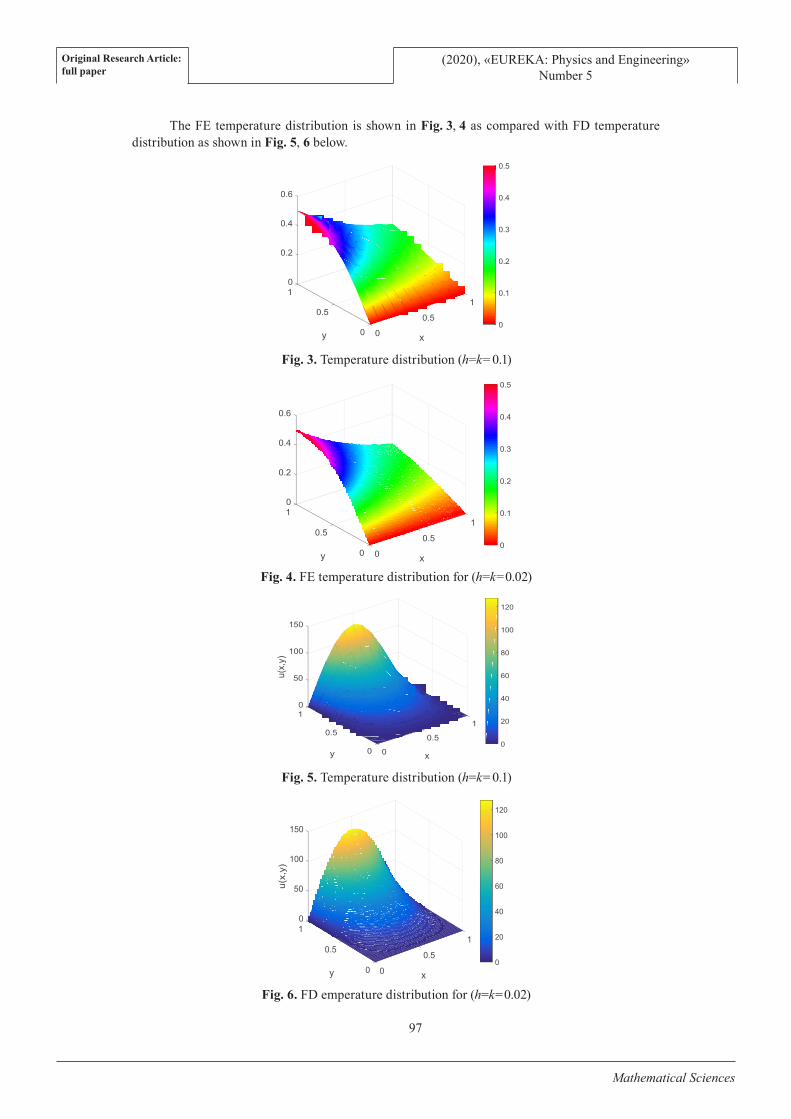
Example 2. Consider a varied boundary heat conduction plate problem in Fig. 7 below, with
( )2
1
1 1x+ + °C temperature at the top boundary and bottom boundary temperature 0 °C. The left
and right boundary temperatures are 21
y
y+ °C and
24
y
y+ °C respectively as shown in the figure
below, with the exact solution given as
( )( )2 2.
1exact
yT
x y=
+ +
Fig. 7. 2D rectangular plate with its boundaries at different temperatures. (Dirichlet condition)
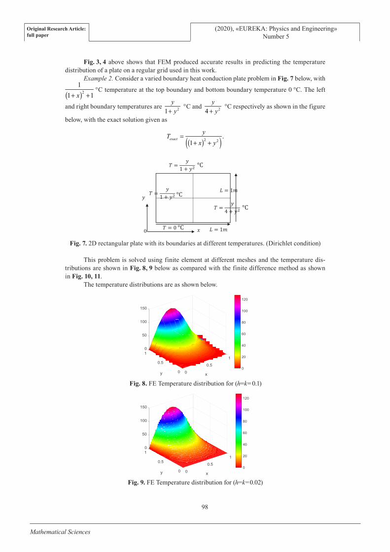
This problem is solved using finite element at different meshes and the temperature dis-
tributions are shown in Fig. 8, 9 below as compared with the finite difference method as shown
in Fig. 10, 11.
The temperature distributions are as shown below.
Fig. 8. FE Temperature distribution for (h=k=0.1)
Fig. 9. FE Temperature distribution for (h=k=0.02)
𝑦𝑦
𝑥𝑥 0
𝑇𝑇 = 𝑦𝑦4 + 𝑦𝑦2 °C
𝑇𝑇 = 𝑦𝑦1 + 𝑦𝑦2 °C
𝑇𝑇 = 0 °C
𝑇𝑇 = 𝑦𝑦1 + 𝑦𝑦2 °C
𝐿𝐿 = 1𝑚𝑚
𝐿𝐿 = 1𝑚𝑚
Original Research Article:
full paper(2020), «EUREKA: Physics and Engineering»
Number 5
99
Mathematical Sciences
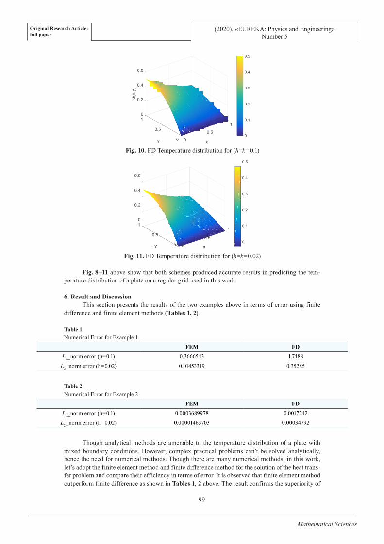
Fig. 10. FD Temperature distribution for (h=k=0.1)
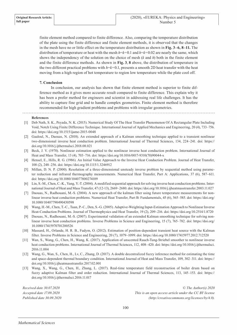
Fig. 11. FD Temperature distribution for (h=k=0.02)
Fig. 8–11 above show that both schemes produced accurate results in predicting the tem-
perature distribution of a plate on a regular grid used in this work.
6. Result and Discussion
This section presents the results of the two examples above in terms of error using finite
difference and finite element methods (Tables 1, 2).
Table 1
Numerical Error for Example 1
FEM FD
L2_norm error (h=0.1) 0.3666543 1.7488
L2_norm error (h=0.02) 0.01453319 0.35285
Table 2
Numerical Error for Example 2
FEM FD
L2_norm error (h=0.1) 0.0003689978 0.0017242
L2_norm error (h=0.02) 0.00001463703 0.00034792
Though analytical methods are amenable to the temperature distribution of a plate with
mixed boundary conditions. However, complex practical problems can’t be solved analytically,
hence the need for numerical methods. Though there are many numerical methods, in this work,
let’s adopt the finite element method and finite difference method for the solution of the heat trans-
fer problem and compare their efficiency in terms of error. It is observed that finite element method
outperform finite difference as shown in Tables 1, 2 above. The result confirms the superiority of
Original Research Article:
full paper
(2020), «EUREKA: Physics and Engineering»
Number 5
100
Mathematical Sciences
finite element method compared to finite difference. Also, comparing the temperature distribution
of the plate using the finite difference and finite element methods, it is observed that the changes
in the mesh have no or little effect on the temperature distribution as shown in Fig. 3–6, 8–11. The
distribution of temperature or heat with the mesh h=k=0.1 and h=k=0.02 are nearly the same, which shows the independency of the solution on the choice of mesh (k and h) both in the finite element
and the finite difference methods. As shown in Fig. 3, 8 above, the distribution of temperature in
the two different practical problems with h=k=0.1, presents a smooth 2D heat transfer with the heat moving from a high region of hot temperature to region low temperature while the plate cool off.
7. Conclusion
In conclusion, our analysis has shown that finite element method is superior to finite dif-
ference method as it gives more accurate result compared to finite difference. This explain why it
has been a prefer method for engineers and scientist in addressing real life challenges. It has the
ability to capture fine grid and to handle complex geometries. Finite element method is therefore
recommended for high gradient problems and problems with irregular geometries.
References
[1] Deb Nath, S. K., Peyada, N. K. (2015). Numerical Study Of The Heat Transfer Phenomenon Of A Rectangular Plate Including
Void, Notch Using Finite Difference Technique. International Journal of Applied Mechanics and Engineering, 20 (4), 733–756.
doi: https://doi.org/10.1515/ijame-2015-0048
[2] Gaaloul, N., Daouas, N. (2018). An extended approach of a Kalman smoothing technique applied to a transient nonlinear
two-dimensional inverse heat conduction problem. International Journal of Thermal Sciences, 134, 224–241. doi: https://
doi.org/10.1016/j.ijthermalsci.2018.08.021
[3] Beck, J. V. (1970). Nonlinear estimation applied to the nonlinear inverse heat conduction problem. International Journal of
Heat and Mass Transfer, 13 (4), 703–716. doi: https://doi.org/10.1016/0017-9310(70)90044-x
[4] Hensel, E., Hills, R. G. (1986). An Initial Value Approach to the Inverse Heat Conduction Problem. Journal of Heat Transfer,
108 (2), 248–256. doi: https://doi.org/10.1115/1.3246912
[5] Millan, D. N. P. (2000). Resolution of a three-dimensional unsteady inverse problem by sequential method using parame-
ter reduction and infrared thermography measurements. Numerical Heat Transfer, Part A: Applications, 37 (6), 587–611.
doi: https://doi.org/10.1080/104077800274109
[6] Lin, S.-M., Chen, C.-K., Yang, Y.-T. (2004). A modified sequential approach for solving inverse heat conduction problems. Inter-
national Journal of Heat and Mass Transfer, 47 (12-13), 2669–2680. doi: https://doi.org/10.1016/j.ijheatmasstransfer.2003.11.027
[7] Daouas, N., Radhouani, M.-S. (2004). A new approach of the kalman filter using future temperature measurements for non-
linear inverse heat conduction problems. Numerical Heat Transfer, Part B: Fundamentals, 45 (6), 565–585. doi: https://doi.org/
10.1080/10407790490430598
[8] Wang, H.-M., Chen, T.-C., Tuan, P.-C., Den, S.-G. (2005). Adaptive-Weighting Input-Estimation Approach to Nonlinear Inverse
Heat-Conduction Problems. Journal of Thermophysics and Heat Transfer, 19 (2), 209–216. doi: https://doi.org/10.2514/1.8720
[9] Daouas, N., Radhouani, M.-S. (2007). Experimental validation of an extended Kalman smoothing technique for solving non-
linear inverse heat conduction problems. Inverse Problems in Science and Engineering, 15 (7), 765–782. doi: https://doi.org/
10.1080/17415970701200526
[10] Massard, H., Orlande, H. R. B., Fudym, O. (2012). Estimation of position-dependent transient heat source with the Kalman
filter. Inverse Problems in Science and Engineering, 20 (7), 1079–1099. doi: https://doi.org/10.1080/17415977.2012.712520
[11] Wan, S., Wang, G., Chen, H., Wang, K. (2017). Application of unscented Rauch-Tung-Striebel smoother to nonlinear inverse
heat conduction problems. International Journal of Thermal Sciences, 112, 408–420. doi: https://doi.org/10.1016/j.ijthermalsci.
2016.11.004
[12] Wang, G., Wan, S., Chen, H., Lv, C., Zhang, D. (2017). A double decentralized fuzzy inference method for estimating the time
and space-dependent thermal boundary condition. International Journal of Heat and Mass Transfer, 109, 302–311. doi: https://
doi.org/10.1016/j.ijheatmasstransfer.2017.02.001
[13] Wang, X., Wang, G., Chen, H., Zhang, L. (2017). Real-time temperature field reconstruction of boiler drum based on
fuzzy adaptive Kalman filter and order reduction. International Journal of Thermal Sciences, 113, 145–153. doi: https://
doi.org/10.1016/j.ijthermalsci.2016.11.017
© The Author(s) 2020
This is an open access article under the CC BY license
(http://creativecommons.org/licenses/by/4.0).
Received date 30.07.2020
Accepted date 17.09.2020
Published date 30.09.2020
Recommended