Finite Element Methods
Two Dimensional Solid
Instructor: Mohamed Abdou Mahran Kasem, Ph.D.
Aerospace Engineering Department
Cairo University

Plane stress
Plane stress is a state of stress in which the normal stress and the shear stresses directed perpendicular to the plane are assumed to be zero.
𝑖. 𝑒. 𝜎𝑧 , 𝜏𝑥𝑧 , 𝜏𝑦𝑧 = 0

Plane strain
Plane strain is a state of strain in which the normal strain and the shear strains directed perpendicular to the plane are assumed to be zero.
𝑖. 𝑒. 𝜀𝑧, 𝛾𝑥𝑧 , 𝛾𝑦𝑧 = 0

Plane stress
As we mentioned before the governing equilibrium equation for elastic, static, linear analysis has the form
න𝑤 𝑖,𝑗 𝜎𝑖𝑗 𝑑Ω = න𝑤𝑖𝑓𝑖 𝑑Ω + 𝐵. 𝑇. 𝜎𝑖𝑗 = 𝐶𝑖𝑗𝑘𝑙𝜀𝑘𝑙 = 𝐶𝑖𝑗𝑘𝑙𝑢𝑘,𝑙 + 𝑢𝑙,𝑘
2= 𝐶𝑖𝑗𝑘𝑙𝑢 𝑖,𝑗

Plane stress
In this case the stress-strain relation is reduced to the form
𝜎11𝜎22𝜎12
=2𝜇 + 𝜆 𝜆 0
𝜆 2𝜇 + 𝜆 00 0 2𝜇
𝜀11𝜀22𝜀12
=𝐸
1 − 𝑣2
1 𝑣 0𝑣 1 0
0 01 − 𝑣
2
𝜀11𝜀22𝜀12
= 𝐃𝛆
λ and μ are Lame´ constants. They are related to the well-known Young’s Modulus (E) and Poisson’s ratio (υ) by
the following relation
𝜆 =𝐸 𝑣
1 + 𝑣 1 − 2𝑣, 𝜇 =
𝐸
2 1 + 𝑣

Plane stress
The strain-displacement relation takes the form
𝐮 = 𝐍𝐔 → 𝛆 = 𝛛𝐍 𝐔 = 𝐁𝐔

Linear triangular element

Linear triangular element
3-node element
In matrix form:

Linear triangular element
Substitute by the BC’s
I
II
By solving the two-set of equations together, one can obtain the shape functions for linear
triangular element

Linear triangular element

Linear triangular element

Linear triangular element
Element strains

Linear triangular element
Element strains
Similarly, we can obtain the other derivatives

Linear triangular element
By substitute in the weak form,
Where B is the strain displacement matrix and D in the material stiffness matrix
depends on the element either plane stress or strain.
න𝑤 𝑖,𝑗 𝜎𝑖𝑗 𝑑Ω = න𝑤𝑖𝑓𝑖 𝑑Ω + 𝐵. 𝑇.
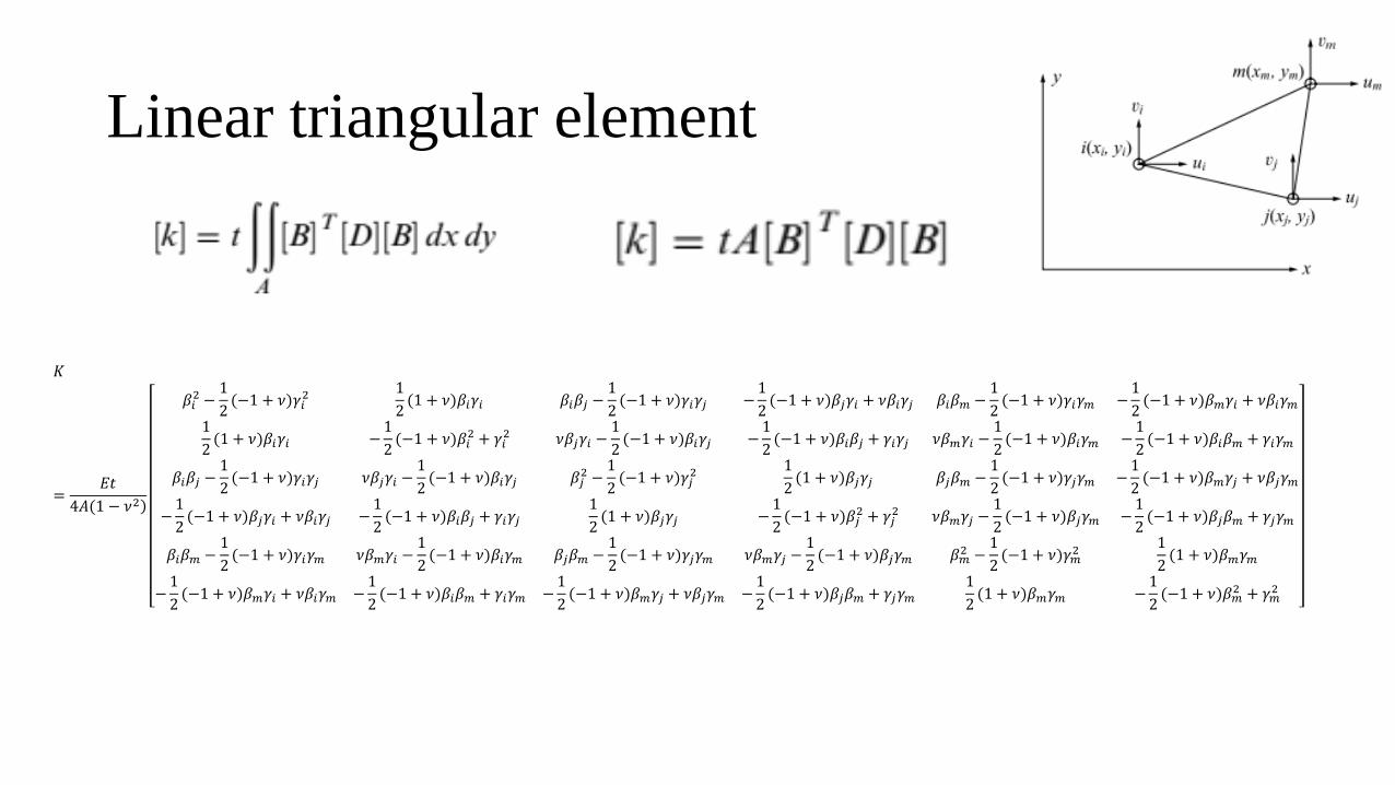
Linear triangular element
𝐾
=𝐸𝑡
ሻ4𝐴(1 − 𝜈2
𝛽𝑖2 −
1
2(−1 + 𝜈ሻ𝛾𝑖
2 1
2(1 + 𝜈ሻ𝛽𝑖𝛾𝑖 𝛽𝑖𝛽𝑗 −
1
2(−1 + 𝜈ሻ𝛾𝑖𝛾𝑗 −
1
2(−1 + 𝜈ሻ𝛽𝑗𝛾𝑖 + 𝜈𝛽𝑖𝛾𝑗 𝛽𝑖𝛽𝑚 −
1
2(−1 + 𝜈ሻ𝛾𝑖𝛾𝑚 −
1
2(−1 + 𝜈ሻ𝛽𝑚𝛾𝑖 + 𝜈𝛽𝑖𝛾𝑚
1
2(1 + 𝜈ሻ𝛽𝑖𝛾𝑖 −
1
2(−1 + 𝜈ሻ𝛽𝑖
2 + 𝛾𝑖2 𝜈𝛽𝑗𝛾𝑖 −
1
2(−1 + 𝜈ሻ𝛽𝑖𝛾𝑗 −
1
2(−1 + 𝜈ሻ𝛽𝑖𝛽𝑗 + 𝛾𝑖𝛾𝑗 𝜈𝛽𝑚𝛾𝑖 −
1
2(−1 + 𝜈ሻ𝛽𝑖𝛾𝑚 −
1
2(−1 + 𝜈ሻ𝛽𝑖𝛽𝑚 + 𝛾𝑖𝛾𝑚
𝛽𝑖𝛽𝑗 −1
2(−1 + 𝜈ሻ𝛾𝑖𝛾𝑗 𝜈𝛽𝑗𝛾𝑖 −
1
2(−1 + 𝜈ሻ𝛽𝑖𝛾𝑗 𝛽𝑗
2 −1
2(−1 + 𝜈ሻ𝛾𝑗
2 1
2(1 + 𝜈ሻ𝛽𝑗𝛾𝑗 𝛽𝑗𝛽𝑚 −
1
2(−1 + 𝜈ሻ𝛾𝑗𝛾𝑚 −
1
2(−1 + 𝜈ሻ𝛽𝑚𝛾𝑗 + 𝜈𝛽𝑗𝛾𝑚
−1
2(−1 + 𝜈ሻ𝛽𝑗𝛾𝑖 + 𝜈𝛽𝑖𝛾𝑗 −
1
2(−1 + 𝜈ሻ𝛽𝑖𝛽𝑗 + 𝛾𝑖𝛾𝑗
1
2(1 + 𝜈ሻ𝛽𝑗𝛾𝑗 −
1
2(−1 + 𝜈ሻ𝛽𝑗
2 + 𝛾𝑗2 𝜈𝛽𝑚𝛾𝑗 −
1
2(−1 + 𝜈ሻ𝛽𝑗𝛾𝑚 −
1
2(−1 + 𝜈ሻ𝛽𝑗𝛽𝑚 + 𝛾𝑗𝛾𝑚
𝛽𝑖𝛽𝑚 −1
2(−1 + 𝜈ሻ𝛾𝑖𝛾𝑚 𝜈𝛽𝑚𝛾𝑖 −
1
2(−1 + 𝜈ሻ𝛽𝑖𝛾𝑚 𝛽𝑗𝛽𝑚 −
1
2(−1 + 𝜈ሻ𝛾𝑗𝛾𝑚 𝜈𝛽𝑚𝛾𝑗 −
1
2(−1 + 𝜈ሻ𝛽𝑗𝛾𝑚 𝛽𝑚
2 −1
2(−1 + 𝜈ሻ𝛾𝑚
21
2(1 + 𝜈ሻ𝛽𝑚𝛾𝑚
−1
2(−1 + 𝜈ሻ𝛽𝑚𝛾𝑖 + 𝜈𝛽𝑖𝛾𝑚 −
1
2(−1 + 𝜈ሻ𝛽𝑖𝛽𝑚 + 𝛾𝑖𝛾𝑚 −
1
2(−1 + 𝜈ሻ𝛽𝑚𝛾𝑗 + 𝜈𝛽𝑗𝛾𝑚 −
1
2(−1 + 𝜈ሻ𝛽𝑗𝛽𝑚 + 𝛾𝑗𝛾𝑚
1
2(1 + 𝜈ሻ𝛽𝑚𝛾𝑚 −
1
2(−1 + 𝜈ሻ𝛽𝑚
2 + 𝛾𝑚2

Example
Evaluate the stiffness matrix for the element shown in Figure. The coordinates
are shown in units of inches. Assume plane stress conditions. Let 𝐸 = 30𝑥106psi,
𝜐 = 0.25, and thickness t = 1 in. Assume the element nodal displacements have been
determined to be 𝑢1 = 0, 𝑣1 = 0.0025 𝑖𝑛, 𝑢2 = 0.0012 𝑖𝑛, 𝑣2 = 0, 𝑢3 = 0, 𝑣3 = 0.0025 𝑖𝑛
Determine the element stresses.

Example

Example

Example

Surface Forces

Surface Forces

Surface Forces
Equivalent nodal forces
Example
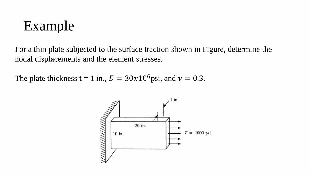
For a thin plate subjected to the surface traction shown in Figure, determine the
nodal displacements and the element stresses.
The plate thickness t = 1 in., 𝐸 = 30𝑥106psi, and 𝜈 = 0.3.

Example
Plate mesh

Example
Calculate element stiffnesses

Example
Calculate element stiffnesses

Example
Calculate element stiffnesses

Example
Calculate element stiffnesses

Example
Calculate element stiffnesses

Example
Calculate element stiffnesses

Example
The global stiffness matrix

Example
After applying the BC’s

Example
Determine the unknown displacements

Example
Comparing to analytical solution
- The analytical solution represents 1-D approximation, while the FE solution represents 2-
D approximation.
- We used a coarse mesh in the FE solution, which results in an inaccurate solution.

Example
Element stresses

Example
Stresses for element 1

Example
Stresses for element 2

This lecture is prepared from: Logan “A first course in the finite element method”
Recommended