2
Fitting Gamma Ranking Models to Soccer Data: Luce’s Choice Axiom and Thurstone’s Law in
Practice
Abstract:
This thesis aims to construct a ranking system measuring the latent variable football ability with random
utility methodologies. We consider discriminal processes that are based on gamma distributions. We model
football match outcomes as normal, logistic and Laplace Thurstone processes and relate these to Luce´s
choice axiom. Numerical optimization of the likelihoods computed through a general linear model produces
parameter estimates. Thurstone´s Case V model, the normal model, is closest to the real ranking based on
ranking correlation measured by Kendall´s tau. Dawkins´ model, the Laplace model, has the highest value for
goodness of fit, measured by the Akaike Information Criterion, due to its ability to model fat tails and a sharp
peak simultaneously. Luce’s model, the logistic distribution, overestimates the thickness of the tails and is too flat
at the peak. Thurstone´s Case V model cannot cope with the excess kurtosis.
Author: Yugesh Raghoenath (333768)
Supervised by: Dr. A.J. Koning
Erasmus School of Economics
Erasmus University
February 2017
3
1. Introduction
In recent years statistical analysis has become increasingly important in sports. In a market that expands and
becomes more competitive year after year, an extra edge might come from such analyses. Trainers, players,
media, bookmakers and gamblers use information, insights and numerous statistics for very different
purposes. Specific examples are scouting future opponents and players or evaluating past performances.
Financial applications include estimating realistic odds as a bookmaker. To do so, it is key to assess the
strengths and weaknesses of teams and players adequately.
Within a competition, players and teams are comparable on many statistics as matches are played amongst
each other. Still, translating the individual statistics to a combined measure of strength or football ability, if
you will, is less trivial; winning matches against stronger opposing teams is a better indicator of high football
ability than winning matches against weaker opponents. Moreover, losing multiple games in a row with
minimal differences and winning one game with a major difference can result in a positive goal deficit. With a
system that estimates aggregate team football abilities correctly, bookmakers quote their odds more
efficiently.
The goal of this research is to create a ranking of teams that allows for a realistic measure of the football
ability. We model the team’s latent football ability pre-match as random variables and the matches as paired
comparisons of these random variables. In this context the team with the highest football ability before the
match has the highest probability of winning the match. This is no fixed value because the difference between
random football abilities is again a random variable. To create an aggregate team football ability model, we
adopt random utility methodologies in a paired comparison setting.
Random utility models are applicable to a range of problems in modelling discrete data. Applications include
measuring chess players skill level, see (Henery, 1992), or measuring the strength of some latent stimuli, such
as facial attractiveness, see (Bauml, 1994). The literature regarding ranking or ordering random objects
according to preferences is extensive. Analyzing and Modelling Rank Data (Marden, 1996) is one of many
books aiming to give a comprehensive overview of important ranking models.
Random utility models consist out of a deterministic part and a random part, the error. The distribution of the
error obviously determines the distribution of the random utility. We model the random football abilities, 𝑋𝑖,
as gamma random variables. Say we are to rank 𝑘 teams, then the times until each team reaches a certain
4
number of points has a gamma distribution. We consider three different classes of gamma ranking models
based on different values for the shape parameter: the class of models when the shape parameter goes to
zero, the class of models when the shape parameter is equal to one and the class of models when the shape
parameter goes to infinity. The error distribution is different for these three cases. These three cases
correspond to the exponential distribution in the first case, the Gumbel distribution in the second case and
the normal distribution in the third case. To facilitate linear models with non-normally distributed errors we
work with general linear models (GLM).
We proceed to model the outcome of soccer matches as discriminal processes as described by the law of
comparative judgment in (Thurstone, 1927). A discriminal process is any process in which comparisons are
made between pairs of a collection of entities with respect to magnitudes of some attribute. The distribution
of differences in football ability, 𝐹(𝑋𝑖 − 𝑋𝑗) is thus what concerns the Thurstone models we consider. 𝐹
determines the distribution of possible outcomes of football matches. Thurstone’s original model, see
(Thurstone, 1928), elaborates on the class of Thurstone models where 𝐹 is the normal distribution. The
gamma ranking models we use imply three distinct classes of Thurstone models; a Thurstone model with
exponential, Gumbel and normally distributed football abilities, 𝑋𝑖. Evidently, this results in different
probability distributions 𝐹 for each of the Thurstone models.
Precisely these three classes of Thurstone models are analyzed in (Yelott, 1977), where the relationship
between Thurstone’s law of comparative judgment, the double exponential distribution and Luce´s choice
axiom (Luce, 1959) is investigated. Luce’s choice axiom is a set of axiomatic foundations. Selection according
to Luce´s Choice Axiom is said to have “independence of irrelevant alternatives” (IIA). This means that
the probability of selecting one item over another from a pool of many items is not affected by the
alternatives in that particular pool. Moreover, that particular probability is independent of the presence or
absence of other items in said pool. To be more precise, the ratio of quantified preferences of these two
items remains the same, while the absolute quantifications of these preferences may differ after adding or
removing items to the pool of alternatives. Section 3.2.3 shows all axioms before going into the practical
applications of the model. Additionally, Appendix C contains notes on the proof of ‘Luce’s Lemma 3’,
independence from irrelevant alternatives.
According to (Yelott, 1977), Thurstone models with exponential random variables are equivalent to Dawkins’
Threshold model for paired comparisons (Dawkins, 1969). In addition, in (Yelott, 1977), derivations show that
every Thurstone model with the Laplace distribution as its difference distribution is equivalent to Dawkins’
model for paired comparisons. Finally, according to (Yelott, 1977) assumptions underlying Dawkins’ model are

5
too strong to be generally true and it seems fair to attribute the success of Dawkins’ model for paired
comparisons to the fact that it happens to be a Thurstone model in this special case.
In (Block & Marschak, 1960) as well as in the proof by Marley and Holman in (Luce & Suppes, 1965) it is
showed that exponential discriminal Thurstone processes are equivalent to the logistic distribution. Therefore
it abides by Luce´s choice axiom. Our third model, Thurstone´s original model, abides by the choice axiom as
well according to (Yelott, 1977).
To model these processes, it is appropriate to draw gamma random variables from the same family but with a
different location shift, see (Stern, 1990). Therefore, we limit our models to cases in which 𝑋𝑖 and 𝑋𝑗 have the
same distribution, while the general model by Thurstone does not require such a restriction. For the
exponential model, we model the outcome of football matches as Laplace random variables with a common
scale equal to one; we mentioned earlier this model is equivalent to Dawkins’ model for paired comparisons.
For the Gumbel model, we apply Luce´s model for paired comparisons; this is the model discussed in (Bradley
& Terry, 1952). Finally, for Thurstone’s normal model, we assume that the continuous preferences are
uncorrelated and have common mean; this model is known as Thurstone´s Case V model (Thurstone, 1928).
In modeling the deterministic part we need to take external settings into account. Soccer matches are
matches between two teams, so we need to work in a paired comparison setting instead of in a setting with
complete experiments, as is the case for horse races for example. The literature on paired comparisons is
extensive and used in a wide array of research topics. In (Wickelmaier & Choisel, 2007) pairwise evaluations
of sounds are analyzed through a standard Bradley-Terry model, while we mentioned earlier that (Bauml,
1994) presents applications involving facial attractiveness. Thurstone's original model is applied to analyze
subjective health outcomes, see (Maydeu-Olivares & Bockenholt, 2008), and to rate the skill level of chess
players, see (Henery, 1992). A detailed overview of the extensions to these two models in a sports context is
given in (Cattelan, 2012).
Evidently, we need to adapt these random utility models to a football match setting. Earlier research shows us
several things: Firstly, in (Agresti, 2002) the Bradley-Terry model is derived with a home advantage because
this turns out to be an important factor empirically. In typical football settings we need to allow for draws. In
(Davidson, 1970) the Bradley-Terry model which allows for draws is derived and in (Henery, 1992) Thurstone's
original model with a home parameter is derived. We do not add the extension that allows for draws, since
we should be able to create a sufficient ranking system without allowing for ties. We believe this is the case,
because the empirical probability that two teams perform exactly the same on numerous metrics such as, the
number of goals scored, the number of goals conceded and the number of points acquired, is extremely slim.

6
This reasoning especially holds when we consider that a football season has more than 200 matches; to our
knowledge, we historically never found such an event. We take this as sufficient advice that we can exclude
the possibility of equal latent football abilities in our model.
We use data on the final scores rather than data on the number of points every team acquired against each
opponent. By not analyzing the number of points received for a certain match instead we prevent that a lot of
information on the difference (or there lack of) is omitted. We work in a regression setting to facilitate our
models. With numerical optimization procedures we optimize the appropriate likelihood functions to find
parameter estimates.
As mentioned we aim to construct a ranking system that adequately assess aggregated team football abilities.
A whole different approach to ranking is minimizing some distance based metric, see (Mallows, 1957).
Distance-based ranking models choose the rankings in such a way that the optimal ranking minimizes the
distance d with respect to some arbitrary metric on the set of all possible rankings. In (Diaconis, 1988) the
most popular distance based metrics are considered, such as the following: Kendall's tau (Kendall, 1948),
Spearman's rho (Spearman, 1904), Spearman's footrule (Spearman, 1904) the Hamming metric (Hamming,
1950), and Cayley's metric (Cayley, 1859). In order to objectively judge our models we adopt two of those
distance based metrics to quantify the distance between our model and the real ranking. We adopt Kendall’s
tau and Spearman’s rho as distance based ranking evaluation criterion. Our main criteria is Kendall's tau. This
correlation coefficient recently gained more interest because it is used in the subsection of finance, risk
management; more specific it is used to describe dependences using copulas. As secondary distance based
metric we use Spearman's rho. Spearman’s rho is nothing else than Pearson’s linear correlation for rankings.
This means testing for independence of rankings is straightforward.
To compare non-nested models we measure their goodness of fit with the Akaike Information Criterion, see
(Akaike, 1973). The Akaike Information Criterion (AIC) is used to measure the goodness of fit, while punishing
the less parsimonious models for their lack of simplicity.
Our main research question becomes: “Among the models by Bradley-Terry, Thurstone´s Case V model and
the model by Dawkins, which random utility regression model fits soccer data best in terms of minimizing the
distance to real rankings according to the Kendall's tau metric?” We investigate whether the widely used
Bradley-Terry model is indeed most fit to model football data. Theoretically, estimates should be similar: A
Thurstone model with logistic distribution is equivalent to Luce’s Choice axiom. Moreover, the difference
distribution of the exponential distribution and the double exponential distribution explicitly show similarities.

7
Furthermore we look into the possible addition of a home advantage effect and how adding this parameter
changes our model in terms of uncertainty and bias.
The data we use to answer this question consists out of all matches played during the season 2013/2014 in
the highest professional Dutch soccer league, the Dutch Eredivisie. This competition can be viewed as a
balanced design in the sense that every team plays each opponent exactly twice. It is important to note that
every team only plays each team once at home (and thus only once away).
This research is a valuable extension to the existing literature in the sense that the comparison of these three
gamma ranking models has not been performed in a football setting, to our knowledge. Moreover we present
a complete framework to model the latent football abilities, which is easily extendable with for example other
external effects, such as team experience or team synergy.
We find that Thurstone’s Case V model outperforms the model by Dawkins’ and Bradley-Terry in terms of
mimicking the real ranking measured in ranking correlation by Kendall´s tau. Moreover all three models are
capable of measuring the latent football ability adequately. This is underlined by the fact that they have a
significant amount of rank correlation with the real ranking as well as among themselves, measured by
Kendall´s tau and Spearman´s rho. This agrees with derivations regarding the similarity between Dawkins’
model and the Bradley-Terry model, see (Yelott, 1977) and earlier findings in (Luce, 1959).
The goodness of fit, measured by AIC, suggests Dawkins´ model, the laplace model, is the best fit because of
its ability to model fat tails as well as a sharp peak. Thurstone’s Case V model, the normal model, lacks the
first of these abilities and the model by Bradley and Terry, the logistic model, lacks the second of these
abilities. We estimate a positive home effect which is showed to be an important extension to model the
latent football abilities.
Further research could investigate how the skill of the individual team players and the number of matches
they have played together, or synergy if you will, affect the team’s skill pre-game. Other extensions include
adding parameters for a team’s experience or even dependence among consecutive games. In (Cattelan,
2009) it is shown how to deal with the dependence among the performances of a team. To incorporate these
effects one should collect (or construct) the appropriate data and reformulate the likelihoods we specify in
Section 3.3. The distributions we consider as difference distributions have in common that they are all
symmetrical. This essentially means that positive deviations and negative deviations from the point estimate
of the match outcome imply the same probability if the absolute deviation is the same. A straight forward
way to extend this research is by evaluating the performance of asymmetric distributions.

8
The proceeding sections of this thesis are structured in the following way. In Section 2 we cover aspects of
our data. Section 3 extensively elaborates on the theory on GLM, gamma models and our methodology
regarding creating and evaluating ranking systems. In Section 4 we show parameter estimates for the football
abilities and evaluation metrics for our models. Finally, Section 5 contains the answer to our research
question in the summary and some possible ways to follow up this research.
9
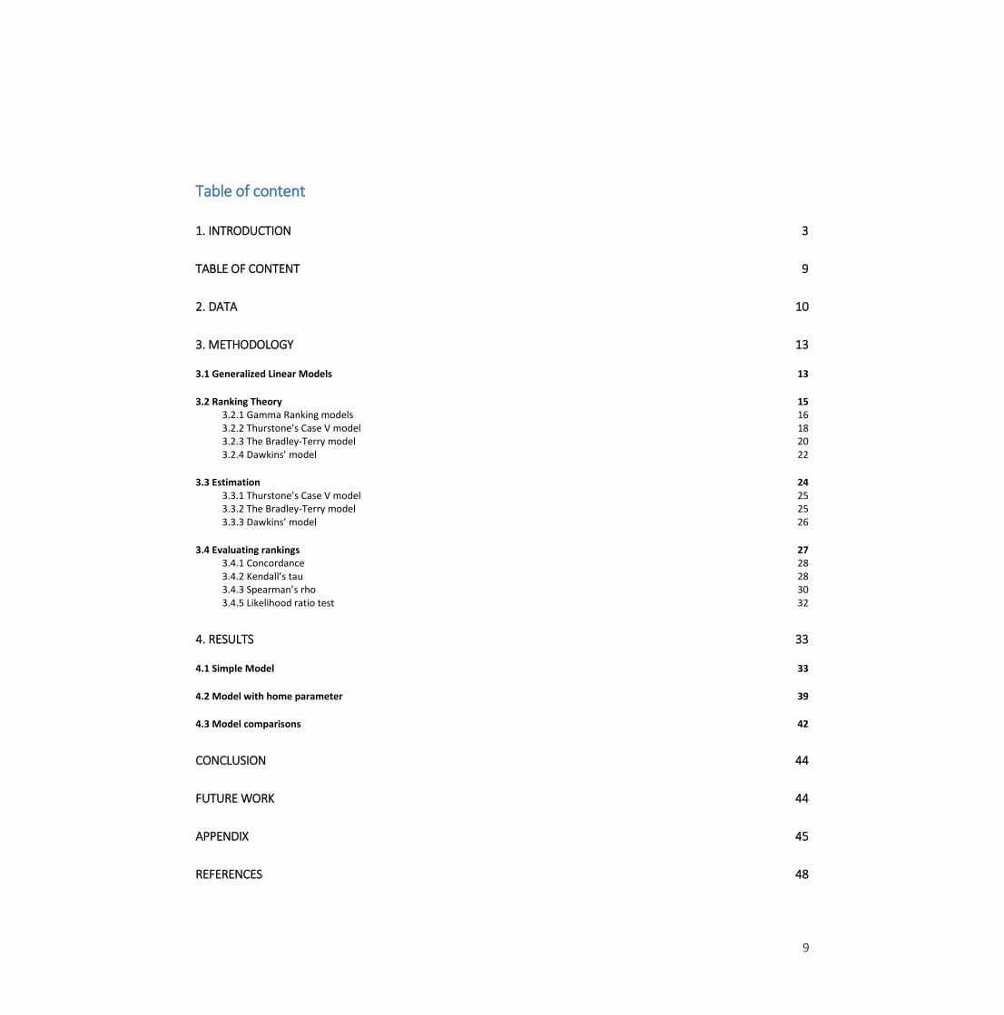
Table of content
1. INTRODUCTION 3
TABLE OF CONTENT 9
2. DATA 10
3. METHODOLOGY 13
3.1 Generalized Linear Models 13
3.2 Ranking Theory 15 3.2.1 Gamma Ranking models 16 3.2.2 Thurstone’s Case V model 18 3.2.3 The Bradley-Terry model 20 3.2.4 Dawkins’ model 22
3.3 Estimation 24 3.3.1 Thurstone’s Case V model 25 3.3.2 The Bradley-Terry model 25 3.3.3 Dawkins’ model 26
3.4 Evaluating rankings 27 3.4.1 Concordance 28 3.4.2 Kendall’s tau 28 3.4.3 Spearman’s rho 30 3.4.5 Likelihood ratio test 32
4. RESULTS 33
4.1 Simple Model 33
4.2 Model with home parameter 39
4.3 Model comparisons 42
CONCLUSION 44
FUTURE WORK 44
APPENDIX 45
REFERENCES 48
10
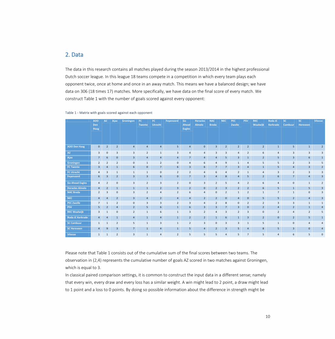
2. Data The data in this research contains all matches played during the season 2013/2014 in the highest professional
Dutch soccer league. In this league 18 teams compete in a competition in which every team plays each
opponent twice, once at home and once in an away match. This means we have a balanced design; we have
data on 306 (18 times 17) matches. More specifically, we have data on the final score of every match. We
construct Table 1 with the number of goals scored against every opponent:
Table 1 - Matrix with goals scored against each opponent
ADO
Den
Haag
AZ Ajax Groningen FC
Twente
FC
Utrecht
Feyenoord Go
Ahead
Eagles
Heracles
Almelo
NAC
Breda
NEC PEC
Zwolle
PSV RKC
Waalwijk
Roda JC
Kerkrade
SC
Cambuur
SC
Hereveen
Vitesse
ADO Den Haag 0 2 2 4 4 4 5 4 0 3 2 2 2 2 1 5 1 2
AZ 3 0 3 3 2 1 3 4 4 3 3 4 2 6 4 3 3 3
Ajax 7 6 0 3 4 4 4 7 4 4 5 3 1 2 5 3 6 1
Groningen 2 2 2 0 1 2 0 4 6 4 9 1 4 5 5 2 3 5
FC Twente 3 4 1 6 0 7 6 3 6 7 7 3 4 1 5 4 3 2
FC Utrecht 4 3 1 1 1 0 2 2 4 6 4 2 1 4 3 2 3 3
Feyenoord 6 3 2 3 3 6 0 7 3 4 8 4 5 2 6 7 4 3
Go Ahead Eagles 4 2 0 3 2 3 2 0 3 2 5 4 2 6 4 0 1 2
Heracles Almelo 4 2 1 1 1 2 3 2 0 2 3 2 2 6 5 1 5 3
NAC Breda 2 3 0 3 2 4 2 6 4 0 2 1 2 1 7 1 0 3
NEC 4 4 2 3 4 2 4 4 2 2 0 4 0 5 5 2 4 3
PEC Zwolle 7 1 2 0 3 3 2 3 4 2 8 0 2 2 3 3 1 1
PSV 5 2 4 2 5 6 1 6 3 3 7 3 0 2 4 2 1 4
RKC Waalwijk 3 1 0 2 1 6 1 3 2 4 3 2 3 0 2 4 2 5
Roda JC Kerkrade 4 4 1 4 1 4 1 2 2 1 6 1 3 2 0 2 5 1
SC Cambuur 1 1 2 5 1 3 1 2 3 0 3 3 1 5 1 0 4 4
SC Hereveen 4 9 3 7 1 4 1 5 4 2 3 5 4 8 5 3 0 4
Vitesse 1 1 2 3 1 4 2 5 5 5 4 5 7 5 4 6 5 0
Please note that Table 1 consists out of the cumulative sum of the final scores between two teams. The
observation in (2,4) represents the cumulative number of goals AZ scored in two matches against Groningen,
which is equal to 3.
In classical paired comparison settings, it is common to construct the input data in a different sense; namely
that every win, every draw and every loss has a similar weight. A win might lead to 2 point, a draw might lead
to 1 point and a loss to 0 points. By doing so possible information about the difference in strength might be

11
omitted; a larger difference in goals typically indicates a larger difference in football ability. We circumvent
this by working with the number of goals rather than the number of points a team received against
opponents.
We investigate the addition of a home parameter which should capture the latent effect of a team being
stronger at home matches. To back up this claim we calculate the percentage of matches won by the home
and away team. Table 2 shows we empirically find a home advantage that is in line with earlier findings in
(Agresti, 2002):
Table 2 - Home advantage
Home Away
% Matches won 39.54 33.01
There is an increase of approximately 6.5% in terms of matches won by a team playing at home.
Please note we cannot use Table 1 for further analyses as this Table does not discriminate among matches
played at home or away. We turned to our raw dataset with the matches in order to perform our further
analysis.
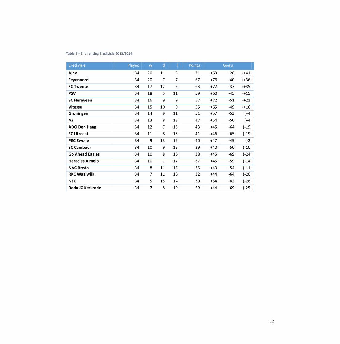
Table 3 shows the final ranking which we use to compare our models to in terms of ranking correlation.
12
Table 3 - End ranking Eredivisie 2013/2014
Eredivisie Played w d l Points Goals
Ajax 34 20 11 3 71 +69 -28 (+41)
Feyenoord 34 20 7 7 67 +76 -40 (+36)
FC Twente 34 17 12 5 63 +72 -37 (+35)
PSV 34 18 5 11 59 +60 -45 (+15)
SC Hereveen 34 16 9 9 57 +72 -51 (+21)
Vitesse 34 15 10 9 55 +65 -49 (+16)
Groningen 34 14 9 11 51 +57 -53 (+4)
AZ 34 13 8 13 47 +54 -50 (+4)
ADO Den Haag 34 12 7 15 43 +45 -64 (-19)
FC Utrecht 34 11 8 15 41 +46 -65 (-19)
PEC Zwolle 34 9 13 12 40 +47 -49 (-2)
SC Cambuur 34 10 9 15 39 +40 -50 (-10)
Go Ahead Eagles 34 10 8 16 38 +45 -69 (-24)
Heracles Almelo 34 10 7 17 37 +45 -59 (-14)
NAC Breda 34 8 11 15 35 +43 -54 (-11)
RKC Waalwijk 34 7 11 16 32 +44 -64 (-20)
NEC 34 5 15 14 30 +54 -82 (-28)
Roda JC Kerkrade 34 7 8 19 29 +44 -69 (-25)
13
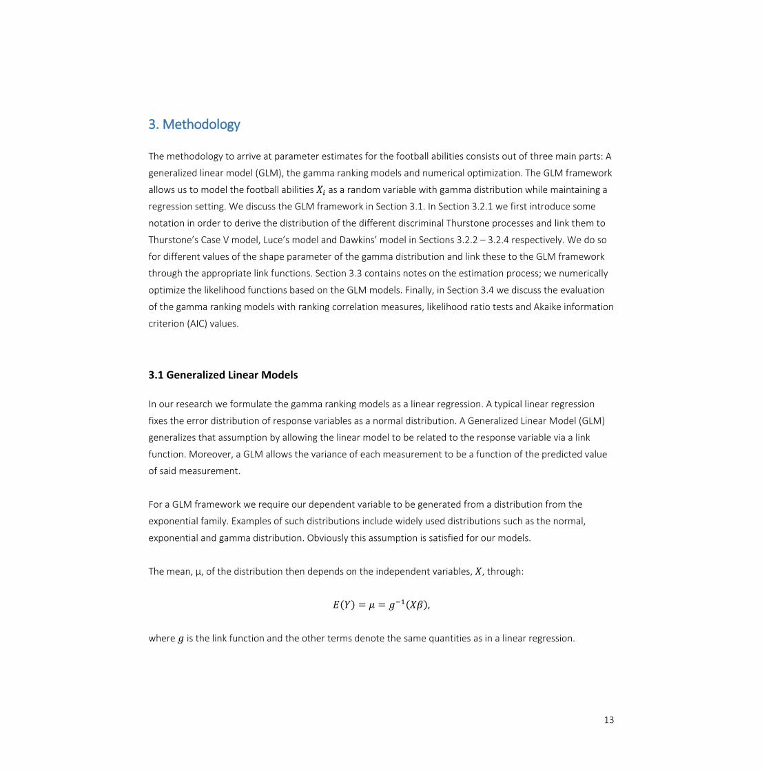
3. Methodology
The methodology to arrive at parameter estimates for the football abilities consists out of three main parts: A
generalized linear model (GLM), the gamma ranking models and numerical optimization. The GLM framework
allows us to model the football abilities 𝑋𝑖 as a random variable with gamma distribution while maintaining a
regression setting. We discuss the GLM framework in Section 3.1. In Section 3.2.1 we first introduce some
notation in order to derive the distribution of the different discriminal Thurstone processes and link them to
Thurstone’s Case V model, Luce’s model and Dawkins’ model in Sections 3.2.2 – 3.2.4 respectively. We do so
for different values of the shape parameter of the gamma distribution and link these to the GLM framework
through the appropriate link functions. Section 3.3 contains notes on the estimation process; we numerically
optimize the likelihood functions based on the GLM models. Finally, in Section 3.4 we discuss the evaluation
of the gamma ranking models with ranking correlation measures, likelihood ratio tests and Akaike information
criterion (AIC) values.
3.1 Generalized Linear Models
In our research we formulate the gamma ranking models as a linear regression. A typical linear regression
fixes the error distribution of response variables as a normal distribution. A Generalized Linear Model (GLM)
generalizes that assumption by allowing the linear model to be related to the response variable via a link
function. Moreover, a GLM allows the variance of each measurement to be a function of the predicted value
of said measurement.
For a GLM framework we require our dependent variable to be generated from a distribution from the
exponential family. Examples of such distributions include widely used distributions such as the normal,
exponential and gamma distribution. Obviously this assumption is satisfied for our models.
The mean, μ, of the distribution then depends on the independent variables, 𝑋, through:
𝐸(𝑌) = 𝜇 = 𝑔−1(𝑋𝛽),
where 𝑔 is the link function and the other terms denote the same quantities as in a linear regression.
14
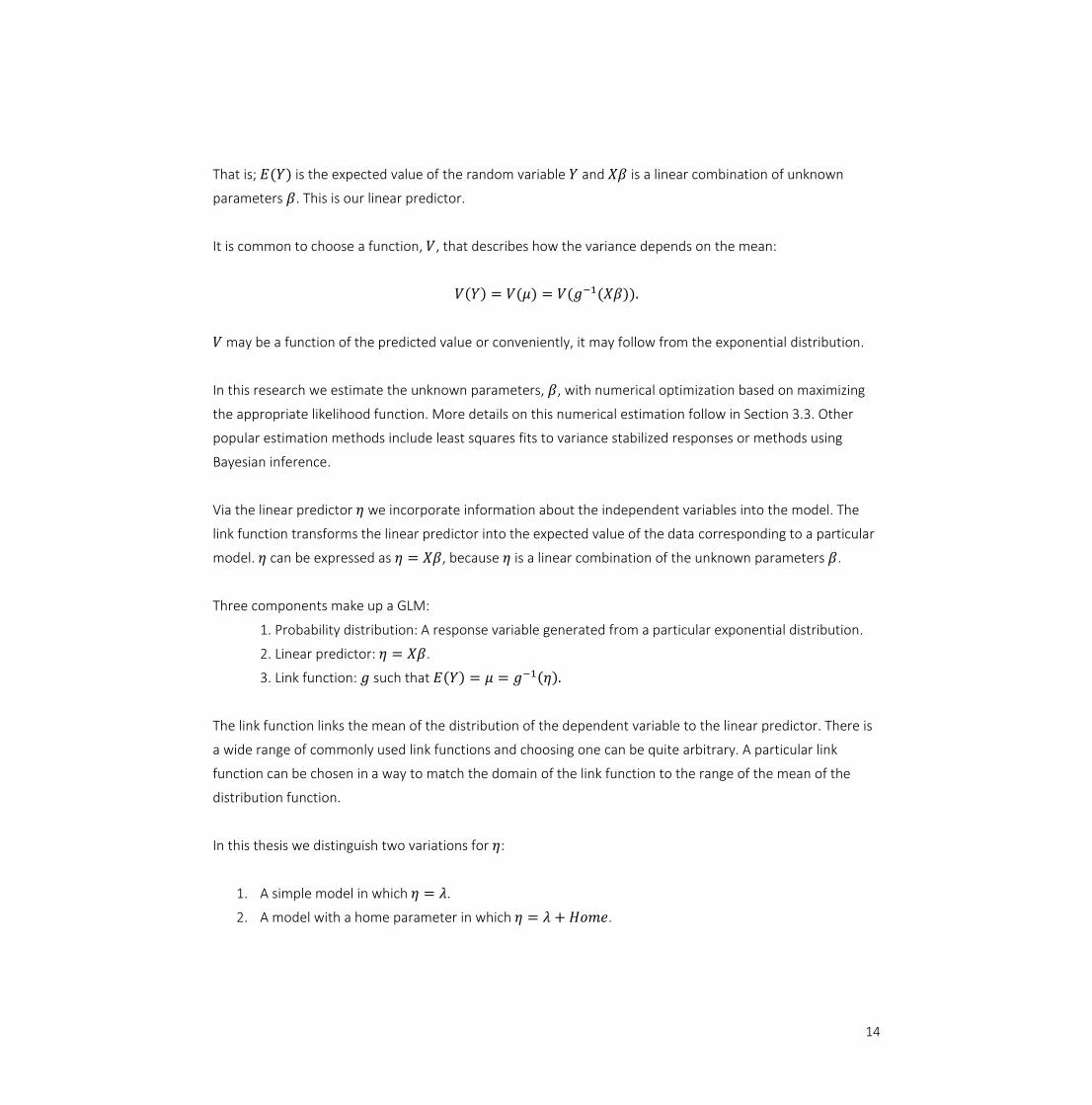
That is; 𝐸(𝑌) is the expected value of the random variable 𝑌 and 𝑋𝛽 is a linear combination of unknown
parameters 𝛽. This is our linear predictor.
It is common to choose a function, 𝑉, that describes how the variance depends on the mean:
𝑉(𝑌) = 𝑉(𝜇) = 𝑉(𝑔−1(𝑋𝛽)).
𝑉 may be a function of the predicted value or conveniently, it may follow from the exponential distribution.
In this research we estimate the unknown parameters, 𝛽, with numerical optimization based on maximizing
the appropriate likelihood function. More details on this numerical estimation follow in Section 3.3. Other
popular estimation methods include least squares fits to variance stabilized responses or methods using
Bayesian inference.
Via the linear predictor 𝜂 we incorporate information about the independent variables into the model. The
link function transforms the linear predictor into the expected value of the data corresponding to a particular
model. 𝜂 can be expressed as 𝜂 = 𝑋𝛽, because 𝜂 is a linear combination of the unknown parameters 𝛽.
Three components make up a GLM:
1. Probability distribution: A response variable generated from a particular exponential distribution.
2. Linear predictor: 𝜂 = 𝑋𝛽.
3. Link function: 𝑔 such that 𝐸(𝑌) = 𝜇 = 𝑔−1(𝜂).
The link function links the mean of the distribution of the dependent variable to the linear predictor. There is
a wide range of commonly used link functions and choosing one can be quite arbitrary. A particular link
function can be chosen in a way to match the domain of the link function to the range of the mean of the
distribution function.
In this thesis we distinguish two variations for 𝜂:
1. A simple model in which 𝜂 = 𝜆.
2. A model with a home parameter in which 𝜂 = 𝜆 + 𝐻𝑜𝑚𝑒.
15
In the both cases we simply estimate the football ability 𝑋𝑖 to have a single parameter football ability. 𝜆 is the
vector of these abilities. The second case however adds a common home parameter to the model.
This parameter is equal for all teams. This additive model results in a fixed increase in football ability
whenever a team is playing at home. So we have a simple model:
𝑋𝑖 = 𝜆𝑖 + 𝜀
(1)
and a model with a home advantage effect:
𝑋𝑖 = 𝜆𝑖 + 𝐻𝑜𝑚𝑒 + 𝜀.
(2)
In Equations (1) and (2) 𝜀 is the error term. We assume 𝑋𝑖 to have gamma distribution and we subsequently
model the outcome of football matches with the discriminal process 𝑋𝑖 − 𝑋𝑗.
In Sections 3.2.1-3.2.4 we derive the distribution of 𝑋𝑖 − 𝑋𝑗 for different values of the shape parameter of the
gamma distribution. We then show that for those distributions, the corresponding models are the normal
model by Thurstone, the model by Bradley-Terry, which is Luce’s model for paired comparisons and the
model by Dawkins for paired comparisons respectively. Finally we choose the appropriate link functions, 𝑔,
based on the distributions 𝑋𝑖 − 𝑋𝑗 and its domain. We compute likelihood functions based on the appropriate
GLM models and numerically optimize those likelihood functions to find estimates for 𝜆𝑖 and 𝐻𝑜𝑚𝑒.
3.2 Ranking Theory
Before we get into the gamma ranking models we need to introduce some notation.
Let 𝜋 = 𝜋1, … , 𝜋𝑘 denote a permutation of 𝑘 teams where team 𝜋𝑝 is ranked (𝑝 = 1, … , 𝑘).
𝜋𝑝−1 is the rank of team 𝑝. The vector 𝜋−1 = [𝜋1
−1, . . ., 𝜋𝑘−1] is thus the vector of ranks. For example; say
𝑘 = 3, 𝜋 = (3 1 2) and say 𝜋−1 = (2 3 1) is the permutation. In this case team 3 has the first ranking, team
1 has the second ranking and team 2 has the third ranking.
We define 𝑝(𝜋) as the distribution of permutations. 𝑃(𝐴) is thus the chance of observing event 𝐴 out of all
outcomes out of 𝑝(𝜋). For example; say we wish to compute the probability that team 𝑠 finishes first:
16
𝑝(𝑠) = 𝑝(𝜋𝑠−1) = ∑ 𝑝(𝜋).
𝜋:𝜋1=𝑠
We generate random permutations Π𝑙 = (Π𝑙1, Π𝑙2, … , Π𝑙𝑘)(𝑙 = 1, … , 𝑛) from the distribution of
permutations (𝜋). These are essentially all different team rankings.
Obviously these rankings can occur in different frequencies. The empirical probability mass function is thus:
𝑝𝑁(𝜋) =
1
𝑁∑ 𝐼(Π𝑚 = 𝜋)
𝑁
𝑚=1
,
where 𝐼 is the indicator function which is equal to 1 if 𝐼(𝐴) occurs and 0 otherwise.
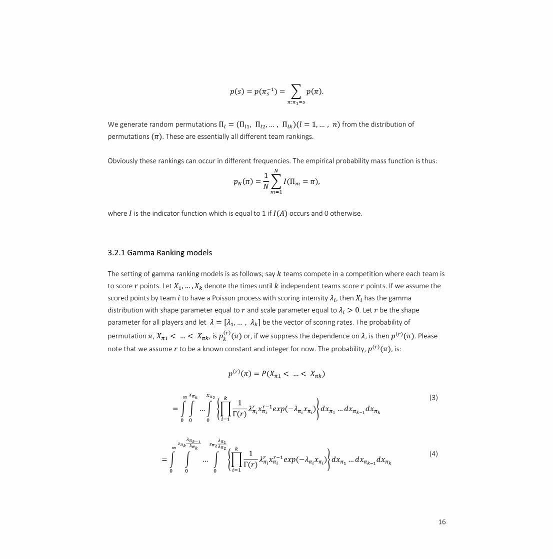
3.2.1 Gamma Ranking models
The setting of gamma ranking models is as follows; say 𝑘 teams compete in a competition where each team is
to score 𝑟 points. Let 𝑋1, … , 𝑋𝑘 denote the times until 𝑘 independent teams score 𝑟 points. If we assume the
scored points by team 𝑖 to have a Poisson process with scoring intensity 𝜆𝑖, then 𝑋𝑖 has the gamma
distribution with shape parameter equal to 𝑟 and scale parameter equal to 𝜆𝑖 > 0. Let 𝑟 be the shape
parameter for all players and let 𝜆 = [𝜆1, … , 𝜆𝑘] be the vector of scoring rates. The probability of
permutation 𝜋, 𝑋𝜋1 < … < 𝑋𝜋𝑘, is 𝑝𝜆(𝑟)
(𝜋) or, if we suppress the dependence on 𝜆, is then 𝑝(𝑟)(𝜋). Please
note that we assume 𝑟 to be a known constant and integer for now. The probability, 𝑝(𝑟)(𝜋), is:
𝑝(𝑟)(𝜋) = 𝑃(𝑋𝜋1 < … < 𝑋𝜋𝑘)
= ∫ ∫ … ∫ {∏1
Γ(𝑟)𝜆𝜋𝑖
𝑟 𝑥𝜋𝑖
𝑟−1𝑒𝑥𝑝 (−𝜆𝜋𝑖𝑥𝜋𝑖
)
𝑘
𝑖=1
} 𝑑𝑥𝜋1… 𝑑𝑥𝜋𝑘−1
𝑑𝑥𝜋𝑘
𝑥𝜋2
0
𝑥𝜋𝑘
0
∞
0
(3)
= ∫ ∫ … ∫ {∏1
Γ(𝑟)𝜆𝜋𝑖
𝑟 𝑥𝜋𝑖
𝑟−1𝑒𝑥𝑝 (−𝜆𝜋𝑖𝑥𝜋𝑖
)
𝑘
𝑖=1
} 𝑑𝑥𝜋1… 𝑑𝑥𝜋𝑘−1
𝑑𝑥𝜋𝑘
𝑧𝜋2
𝜆𝜋1𝜆𝜋2
0
𝑧𝜋𝑘
𝜆𝜋𝑘−1𝜆𝜋𝑘
0
∞
0
(4)
17
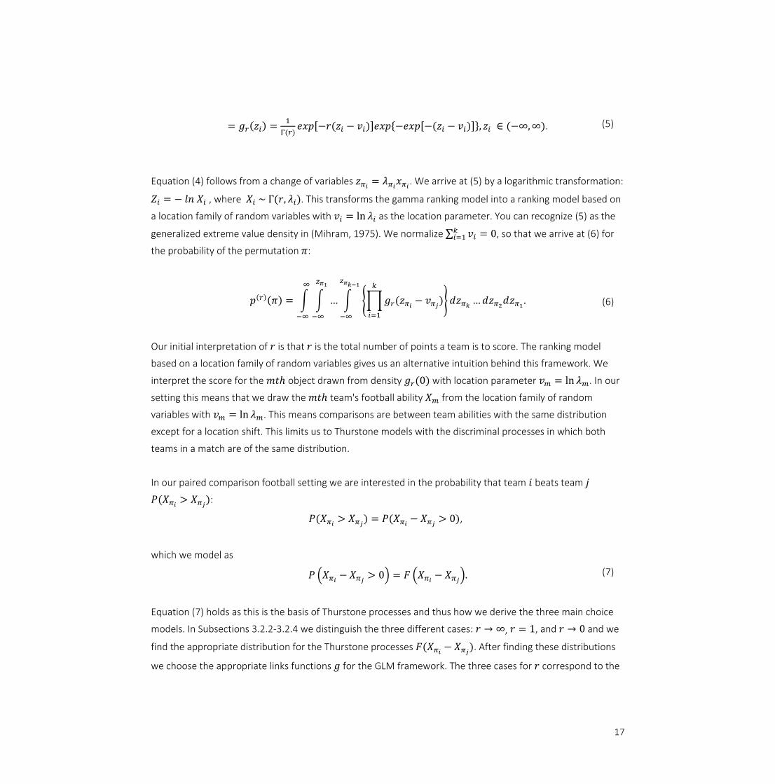
= 𝑔𝑟(𝑧𝑖) =1
Γ(𝑟)𝑒𝑥𝑝[−𝑟(𝑧𝑖 − 𝑣𝑖)]𝑒𝑥𝑝{−𝑒𝑥𝑝[−(𝑧𝑖 − 𝑣𝑖)]}, 𝑧𝑖 ∈ (−∞, ∞).
(5)
Equation (4) follows from a change of variables 𝑧𝜋𝑖= 𝜆𝜋𝑖
𝑥𝜋𝑖. We arrive at (5) by a logarithmic transformation:
𝑍𝑖 = − 𝑙𝑛 𝑋𝑖 , where 𝑋𝑖 ~ Γ(𝑟, 𝜆𝑖). This transforms the gamma ranking model into a ranking model based on
a location family of random variables with 𝑣𝑖 = ln 𝜆𝑖 as the location parameter. You can recognize (5) as the
generalized extreme value density in (Mihram, 1975). We normalize ∑ 𝑣𝑖𝑘𝑖=1 = 0, so that we arrive at (6) for
the probability of the permutation 𝜋:
𝑝(𝑟)(𝜋) = ∫ ∫ … ∫ {∏ 𝑔𝑟(𝑧𝜋𝑖− 𝑣𝜋𝑗
)
𝑘
𝑖=1
} 𝑑𝑧𝜋𝑘… 𝑑𝑧𝜋2
𝑑𝑧𝜋1
𝑧𝜋𝑘−1
−∞
𝑧𝜋1
−∞
∞
−∞
.
(6)
Our initial interpretation of 𝑟 is that 𝑟 is the total number of points a team is to score. The ranking model
based on a location family of random variables gives us an alternative intuition behind this framework. We
interpret the score for the 𝑚𝑡ℎ object drawn from density 𝑔𝑟(0) with location parameter 𝑣𝑚 = ln 𝜆𝑚. In our
setting this means that we draw the 𝑚𝑡ℎ team's football ability 𝑋𝑚 from the location family of random
variables with 𝑣𝑚 = ln 𝜆𝑚. This means comparisons are between team abilities with the same distribution
except for a location shift. This limits us to Thurstone models with the discriminal processes in which both
teams in a match are of the same distribution.
In our paired comparison football setting we are interested in the probability that team 𝑖 beats team 𝑗
𝑃(𝑋𝜋𝑖> 𝑋𝜋𝑗
):
𝑃(𝑋𝜋𝑖> 𝑋𝜋𝑗
) = 𝑃(𝑋𝜋𝑖− 𝑋𝜋𝑗
> 0),
which we model as
𝑃 (𝑋𝜋𝑖− 𝑋𝜋𝑗
> 0) = 𝐹 (𝑋𝜋𝑖− 𝑋𝜋𝑗
).
(7)
Equation (7) holds as this is the basis of Thurstone processes and thus how we derive the three main choice
models. In Subsections 3.2.2-3.2.4 we distinguish the three different cases: 𝑟 → ∞, 𝑟 = 1, and 𝑟 → 0 and we
find the appropriate distribution for the Thurstone processes 𝐹(𝑋𝜋𝑖− 𝑋𝜋𝑗
). After finding these distributions
we choose the appropriate links functions 𝑔 for the GLM framework. The three cases for 𝑟 correspond to the
18
three preference models (by Thurstone, Luce and Dawkins respectively). Please note that we may drop 𝜋
from our notation, so that we have 𝐹(𝑋𝑖 − 𝑋𝑗).
3.2.2 Thurstone’s Case V model
Thurstone's model scales a collection of stimuli based on paired comparisons. In our case this means that by
evaluating all football matches between two teams, the law of comparative judgment estimates scaled values
of the latent football ability such that we can make comparisons between all teams.
In his original model Thurstone assumes items can be compared on one metric, in our case 𝑋𝑖. Moreover, a
discriminal process 𝐹(𝑋𝑖 − 𝑋𝑗), which is normally distributed, determines the outcome of the comparison.
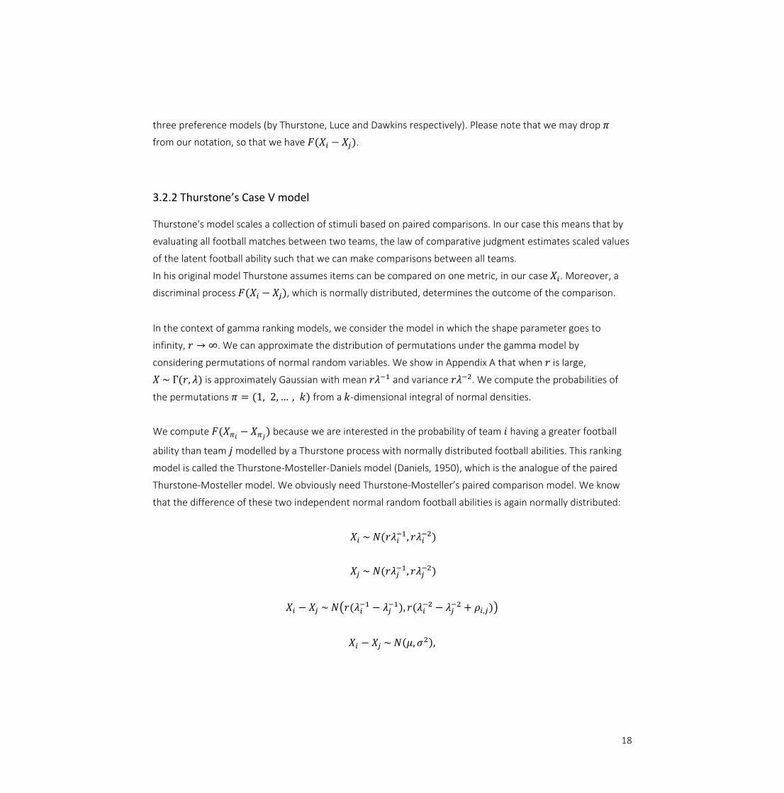
In the context of gamma ranking models, we consider the model in which the shape parameter goes to
infinity, 𝑟 → ∞. We can approximate the distribution of permutations under the gamma model by
considering permutations of normal random variables. We show in Appendix A that when 𝑟 is large,
𝑋 ~ Γ(𝑟, 𝜆) is approximately Gaussian with mean 𝑟𝜆−1 and variance 𝑟𝜆−2. We compute the probabilities of
the permutations 𝜋 = (1, 2, … , 𝑘) from a 𝑘-dimensional integral of normal densities.
We compute 𝐹(𝑋𝜋𝑖− 𝑋𝜋𝑗
) because we are interested in the probability of team 𝑖 having a greater football
ability than team 𝑗 modelled by a Thurstone process with normally distributed football abilities. This ranking
model is called the Thurstone-Mosteller-Daniels model (Daniels, 1950), which is the analogue of the paired
Thurstone-Mosteller model. We obviously need Thurstone-Mosteller’s paired comparison model. We know
that the difference of these two independent normal random football abilities is again normally distributed:
𝑋𝑖 ~ 𝑁(𝑟𝜆𝑖−1, 𝑟𝜆𝑖
−2)
𝑋𝑗 ~ 𝑁(𝑟𝜆𝑗−1, 𝑟𝜆𝑗
−2)
𝑋𝑖 − 𝑋𝑗 ~ 𝑁(𝑟(𝜆𝑖−1 − 𝜆𝑗
−1), 𝑟(𝜆𝑖−2 − 𝜆𝑗
−2 + 𝜌𝑖,𝑗))
𝑋𝑖 − 𝑋𝑗 ~ 𝑁(𝜇, 𝜎2),
19
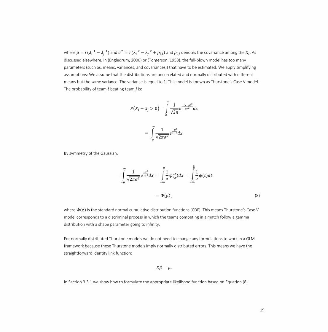
where 𝜇 = 𝑟(𝜆𝑖−1 − 𝜆𝑗
−1) and 𝜎2 = 𝑟(𝜆𝑖−2 − 𝜆𝑗
−2 + 𝜌𝑖,𝑗) and 𝜌𝑖,𝑗 denotes the covariance among the 𝑋𝑖. As
discussed elsewhere, in (Engledrum, 2000) or (Torgerson, 1958), the full-blown model has too many
parameters (such as, means, variances, and covariances,) that have to be estimated. We apply simplifying
assumptions: We assume that the distributions are uncorrelated and normally distributed with different
means but the same variance. The variance is equal to 1. This model is known as Thurstone's Case V model.
The probability of team 𝑖 beating team 𝑗 is:
𝑃(𝑋𝑖 − 𝑋𝑗 > 0) = ∫
1
√2𝜋𝑒
−(𝑥−𝜇)2
2𝜎2 𝑑𝑥
∞
0
= ∫
1
√2𝜋𝜎2𝑒
−𝑥2
2𝜎2𝑑𝑥
∞
−𝜇
.
By symmetry of the Gaussian,
= ∫1
√2𝜋𝜎2𝑒
−𝑥2
2𝜎2𝑑𝑥
∞
−𝜇
= ∫1
𝜎𝜙(
𝑥
𝜎)𝑑𝑥
𝜇
−∞
= ∫1
𝜎𝜙(𝑡)𝑑𝑡
𝜇𝜎
−∞
= Φ(µ) , (8)
where Φ(𝑧) is the standard normal cumulative distribution functions (CDF). This means Thurstone’s Case V
model corresponds to a discriminal process in which the teams competing in a match follow a gamma
distribution with a shape parameter going to infinity.
For normally distributed Thurstone models we do not need to change any formulations to work in a GLM
framework because these Thurstone models imply normally distributed errors. This means we have the
straightforward identity link function:
𝑋𝛽 = 𝜇.
In Section 3.3.1 we show how to formulate the appropriate likelihood function based on Equation (8).
20
3.2.3 The Bradley-Terry model
We model the gamma ranking model with 𝑟 = 1 as Luce’s model. If this assumption regarding the shape
parameter holds, (6) is equal to the extreme value distribution. Again, we model the outcome of football
matches as Thurstone processes: 𝐹(𝑋𝜋𝑖− 𝑋𝜋𝑗
). In Appendix B we show that the difference 𝑋𝜋𝑖− 𝑋𝜋𝑗
is
logistic if 𝑋𝜋𝑖 and 𝑋𝜋𝑗
are Gumbel distributed quantities. In the introduction we refer to (Block & Marschak,
1960) and Holman and Marley cited by (Luce & Suppes, 1965) as alternative proof of this fact. Moreover, if
this is the case, the Thurstone process 𝐹(𝑋𝜋𝑖− 𝑋𝜋𝑗
) is equivalent to Luce’s model.
Luce’s model was introduced to study behavior. Before going into detail on the practical model and its
estimation, we first show the assumptions underlying Luce’s model:
D1. Let there be four sets 𝑅, 𝑆, 𝑇 𝑎𝑛𝑑 𝑈, such that 𝑅 ⊂ 𝑆 ⊂ 𝑇 ⊂ 𝑈.
D2. Let 𝑥, 𝑦, 𝑧 ∈ 𝑇.
D3. Let 𝑃(𝑥, 𝑦) be the probability of choosing 𝑥 instead of 𝑦, where
0 < 𝑃(𝑥, 𝑦) < 1.
D4. 𝑃𝑠(𝑅) is the probability of choosing 𝑅 given choice from among alternatives in 𝑆.
The Choice Axiom then states:
(i) 𝑃𝑇(𝑅) = 𝑃𝑠(𝑅)𝑃𝑇(𝑆).
(ii) 𝐼𝑓 𝑃(𝑥, 𝑦) = 0 for some 𝑥, 𝑦 ∈ 𝑇, 𝑃𝑇(𝑆) = 𝑃𝑇−{𝑋}(𝑆 − {𝑋}).
The choice axiom defines the relationship of how choices within subsets are related in the context of an
individual making choices under uncertainty. The well-known implication of the choice axiom is Lemma 3:
Independence of irrelevant alternatives (IIA). This Lemma states that the relative probability of choosing
alternatives is invariant to the composition of the larger set of alternatives. Again, the ratio is invariant, not
the probabilities themselves. Another way of stating the same fact is that the log-odds of two choices are
constant: 𝑙𝑜𝑔(𝑃𝑠(𝑋) − 𝑃𝑠(𝑌)) = 𝑐. We give the proof for Lemma 3 in Appendix C.
We compute the probability of the permutation 𝜋, 𝑝(𝑟)(𝜋) = 𝑃(𝑋𝜋1 < … < 𝑋𝜋𝑘), as follows:
21
𝑝(1)(𝜋) =
𝜆𝜋1
∑ 𝜆𝜋𝑠
𝑘𝑝=1
…𝜆𝜋𝑘−1
∑ 𝜆𝜋𝑝
𝑘𝑝=2
𝜆𝜋𝑘
𝜆𝜋𝑘
,
where 𝑝(1)(𝜋) is the probability that 𝑘 independent exponential random variables with means 𝜆1−1, … , 𝜆𝑘
−1 are
ranked according to 𝜋. This probability has an intuitive interpretation of a sequence of rankings. The first
fraction is exactly the probability that 𝑋𝜋1 is the minimum of 𝑘 exponentials if their means are 𝜆𝜋1, … , 𝜆𝜋𝑘
.
This means we rank 𝜋1 as the first player. The second fraction is the probability that 𝑋𝜋2 is the smallest
exponential of 𝑘 − 1 exponential random variables; that is 𝑋𝜋2is the smallest in the set, excluding 𝑋𝜋1
.
In our case, we are working in a soccer setting, which means a match between two competing teams: 𝑘 = 2.
Once again, the probability of team 𝑖 beating team 𝑗 is defined as the probability of team 𝑖 having a greater
random football ability than team 𝑗. This is 𝑃(𝑋𝜋𝑖> 𝑋𝜋𝑗
) or 𝑃(𝑋𝑖 > 𝑋𝑗) if we suppress the dependence on 𝜋.
Bradley and Terry derived the equivalent model for paired comparisons:
𝑃(𝑋𝑖 > 𝑋𝑗) =
𝜆𝑖
𝜆𝑖 + 𝜆𝑗
,
where 𝜆𝑖 and 𝜆𝑗 are the mean football ability of team 𝑋𝑖 and team 𝑋𝑗 respectively.
Bradley and Terry then improved their model by assuming exponential score functions:
𝑃(𝑋𝑖 > 𝑋𝑗) =𝑣𝑖
𝑣𝑖 + 𝑣𝑗
,
(9)
so that 𝑣𝑚 = 𝑒𝑥𝑝(𝜆𝑚) for 𝑚 = 1, 2. Please note that this essentially comes down to estimating a logit model
in a GLM framework, with the logit link function:
𝐿𝑜𝑔𝑃(𝑋𝑖>𝑋𝑗)
𝑃(𝑋𝑗>𝑋𝑖)= 𝑣𝑖 − 𝑣𝑗.
.
This once more underlines the fact that the difference of two Gumbel distributed random football abilities is
logistic.
Based on Equation (9) we formulate the likelihood function in Section 3.3.2.
22
3.2.4 Dawkins’ model
Dawkins´ threshold model assumes that objects in a choice experiment have a latent ´threshold´. The more an
object is preferred, the lower its threshold. More formally, 𝑡1, 𝑡2, … , 𝑡𝑘 are the thresholds corresponding to
the choice objects 𝑋1, 𝑋2, … , 𝑋𝑘 and if 𝑡1 < 𝑡2 < ⋯ < 𝑡𝑘, 𝑋1 is most preferred and 𝑋k the least. Furthermore,
𝑉 denotes an “excitation” random variable, with 𝑃(𝑉 ≤ 𝑣) = 𝐻(𝑣). We assume that 𝐻(𝑣) is monotonically
increasing for 𝑣 all and bounded: 0 < 𝐻(𝑣) < 1.
In our setting, when we have a match between team 𝑋i and 𝑋j with 𝑡𝑖 ≤ 𝑡𝑗, the outcome of the match
depends on where 𝑉 is relative to these thresholds: If 𝑉 < 𝑡𝑖 ≤ 𝑡𝑗, simply draw another sample of 𝑉.
If 𝑡𝑖 < 𝑉 ≤ 𝑡𝑗, team 𝑖 beats team 𝑗. If 𝑡𝑖 ≤ 𝑡𝑗 < 𝑉, team 𝑖 and team 𝑗 have a 50 percent chance of winning the
match. Dawkins showed that the probability of team 𝑖 beating team 𝑘, according to this model, in a complete
system is equal to:
𝑝𝑖𝑘 = 1 − 2𝑝𝑘𝑗𝑝𝑗𝑖. (10)
Evidently, we define 𝑝𝑖𝑗 as the probability of team 𝑖 beating team 𝑗 in the case that 𝑉 does not fall below
both thresholds. Moreover Equation (10) only holds when 𝑝𝑖𝑗 ≥ 0.5, 𝑝𝑗𝑘 ≥ 0.5. The remaining cases can be
derived from (10).
According to (Yelott, 1977), Dawkins’ threshold model for paired comparisons is equivalent to a Thurstone
model with a discriminal process of exponential variables.
The gamma ranking model with 𝑟 → 0 results in football abilities, 𝑋𝑖, that are exponential random with mean
𝜀−1 and location parameter ln 𝜆𝑖. In (Stern, 1987) this is shown by considering the 𝐿1 distance between the
densities. This means we can consider the gamma ranking model with 𝑟 sufficiently small by considering
permutations of 𝑘 independent exponential random variables with the same scale parameter 𝜖 and different
location parameters. The equation for the probability of the permutation 𝜋 = (1, 2, … , 𝑘) is then again a
multiple integral of the form of (3).
As mentioned before, we need the distribution of the Thurstone model with a discriminal process 𝑋𝑖 − 𝑋𝑗
based on exponential random variables. We will show that 𝑋𝑖 − 𝑋𝑗 has the double exponential distribution,
or more commonly called the Laplace distribution, if 𝑋𝑚 ~ 𝐸𝑥𝑝(𝜀−1, ln 𝜆𝑚) for 𝑚 ∈ {1, … , 𝑘}.
Say ℎ denotes the PDF of the standard exponential distribution:
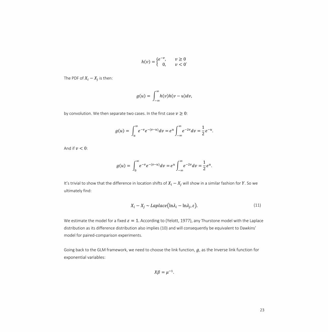
23
ℎ(𝑣) = {𝑒−𝑣 , 𝑣 ≥ 0
0, 𝑣 < 0.
The PDF of 𝑋𝑖 − 𝑋𝑗 is then:
𝑔(𝑢) = ∫ ℎ(𝑣)ℎ(𝑣 − 𝑢)𝑑𝑣
∞
−∞
,
by convolution. We then separate two cases. In the first case 𝑣 ≥ 0:
𝑔(𝑢) = ∫ 𝑒−𝑣𝑒−(𝑣−𝑢)𝑑𝑣 =
∞
𝑢
𝑒𝑢 ∫ 𝑒−2𝑣𝑑𝑣∞
−∞
=1
2𝑒−𝑢.
And if 𝑣 < 0:
𝑔(𝑢) = ∫ 𝑒−𝑣𝑒−(𝑣−𝑢)𝑑𝑣 =
∞
0
𝑒𝑢 ∫ 𝑒−2𝑣𝑑𝑣∞
−∞
=1
2𝑒𝑢.
It’s trivial to show that the difference in location shifts of 𝑋𝑖 − 𝑋𝑗 will show in a similar fashion for 𝑌. So we
ultimately find:
𝑋𝑖 − 𝑋𝑗 ~ 𝐿𝑎𝑝𝑙𝑎𝑐𝑒(ln𝜆𝑖 − ln𝜆𝑗 , 𝜀). (11)
We estimate the model for a fixed 𝜀 = 1. According to (Yelott, 1977), any Thurstone model with the Laplace
distribution as its difference distribution also implies (10) and will consequently be equivalent to Dawkins’
model for paired-comparison experiments.
Going back to the GLM framework, we need to choose the link function, 𝑔, as the Inverse link function for
exponential variables:
𝑋𝛽 = 𝜇−1.
24
Section 3.3.3 contains notes on how to construct the likelihood based on (11).
3.3 Estimation
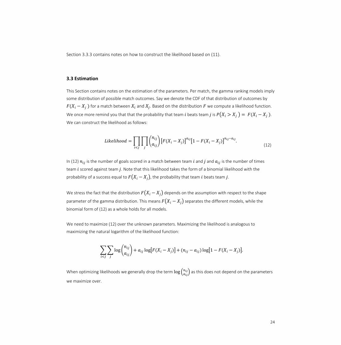
This Section contains notes on the estimation of the parameters. Per match, the gamma ranking models imply
some distribution of possible match outcomes. Say we denote the CDF of that distribution of outcomes by
𝐹(𝑋𝑖 − 𝑋𝑗 ) for a match between 𝑋𝑖 and 𝑋𝑗. Based on the distribution 𝐹 we compute a likelihood function.
We once more remind you that that the probability that team 𝑖 beats team 𝑗 is 𝑃(𝑋𝑖 > 𝑋𝑗 ) = 𝐹(𝑋𝑖 − 𝑋𝑗 ).
We can construct the likelihood as follows:
𝐿𝑖𝑘𝑒𝑙𝑖ℎ𝑜𝑜𝑑 = ∏ ∏ (
𝑛𝑖𝑗
𝑎𝑖𝑗) [𝐹(𝑋𝑖 − 𝑋𝑗)]
𝑎𝑖𝑗[1 − 𝐹(𝑋𝑖 − 𝑋𝑗)]
𝑛𝑖𝑗−𝑎𝑖𝑗.
𝑗𝑖<𝑗
(12)
In (12) 𝑛𝑖𝑗 is the number of goals scored in a match between team 𝑖 and 𝑗 and 𝑎𝑖𝑗 is the number of times
team 𝑖 scored against team 𝑗. Note that this likelihood takes the form of a binomial likelihood with the
probability of a success equal to 𝐹(𝑋𝑖 − 𝑋𝑗), the probability that team 𝑖 beats team 𝑗.
We stress the fact that the distribution 𝐹(𝑋𝑖 − 𝑋𝑗) depends on the assumption with respect to the shape
parameter of the gamma distribution. This means 𝐹(𝑋𝑖 − 𝑋𝑗) separates the different models, while the
binomial form of (12) as a whole holds for all models.
We need to maximize (12) over the unknown parameters. Maximizing the likelihood is analogous to
maximizing the natural logarithm of the likelihood function:
∑ ∑ log (
𝑛𝑖𝑗
𝑎𝑖𝑗) + 𝑎𝑖𝑗 log[𝐹(𝑋𝑖 − 𝑋𝑗)] +
𝑗𝑖<𝑗
(𝑛𝑖𝑗 − 𝑎𝑖𝑗) log[1 − 𝐹(𝑋𝑖 − 𝑋𝑗)].
When optimizing likelihoods we generally drop the term log (𝑛𝑖𝑗𝑎𝑖𝑗
) as this does not depend on the parameters
we maximize over.
25
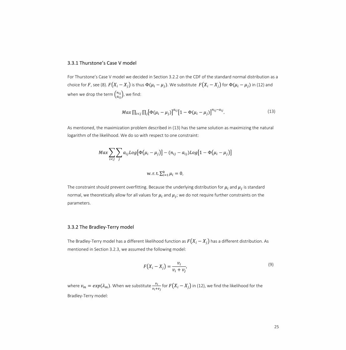
3.3.1 Thurstone’s Case V model
For Thurstone’s Case V model we decided in Section 3.2.2 on the CDF of the standard normal distribution as a
choice for 𝐹, see (8). 𝐹(𝑋𝑖 − 𝑋𝑗) is thus Φ(𝜇𝑖 − 𝜇𝑗). We substitute 𝐹(𝑋𝑖 − 𝑋𝑗) for Φ(𝜇𝑖 − 𝜇𝑗) in (12) and
when we drop the term (𝑛𝑖𝑗𝑎𝑖𝑗
), we find:
𝑀𝑎𝑥 ∏ ∏ [Φ(𝜇𝑖 − 𝜇𝑗)]𝑎𝑖𝑗
[1 − Φ(𝜇𝑖 − 𝜇𝑗)]𝑛𝑖𝑗−𝑎𝑖𝑗
𝑗𝑖<𝑗 .
(13)
As mentioned, the maximization problem described in (13) has the same solution as maximizing the natural
logarithm of the likelihood. We do so with respect to one constraint:
𝑀𝑎𝑥 ∑ ∑ 𝑎𝑖𝑗𝐿𝑜𝑔[Φ(𝜇𝑖 − 𝜇𝑗)] − (𝑛𝑖𝑗 − 𝑎𝑖𝑗)𝐿𝑜𝑔[1 − Φ(𝜇𝑖 − 𝜇𝑗)]
𝑗𝑖<𝑗
w. r. t. ∑ 𝜇𝑖 = 0𝑘𝑖=1 ,
The constraint should prevent overfitting. Because the underlying distribution for 𝜇𝑖 and 𝜇𝑗 is standard
normal, we theoretically allow for all values for 𝜇𝑖 and 𝜇𝑗; we do not require further constraints on the
parameters.
3.3.2 The Bradley-Terry model
The Bradley-Terry model has a different likelihood function as 𝐹(𝑋𝑖 − 𝑋𝑗) has a different distribution. As
mentioned in Section 3.2.3, we assumed the following model:
𝐹(𝑋𝑖 − 𝑋𝑗) =𝑣𝑖
𝑣𝑖 + 𝑣𝑗
, (9)
where 𝑣𝑚 = 𝑒𝑥𝑝(𝜆𝑚). When we substitute 𝑣𝑖
𝑣𝑖+𝑣𝑗 for 𝐹(𝑋𝑖 − 𝑋𝑗) in (12), we find the likelihood for the
Bradley-Terry model:
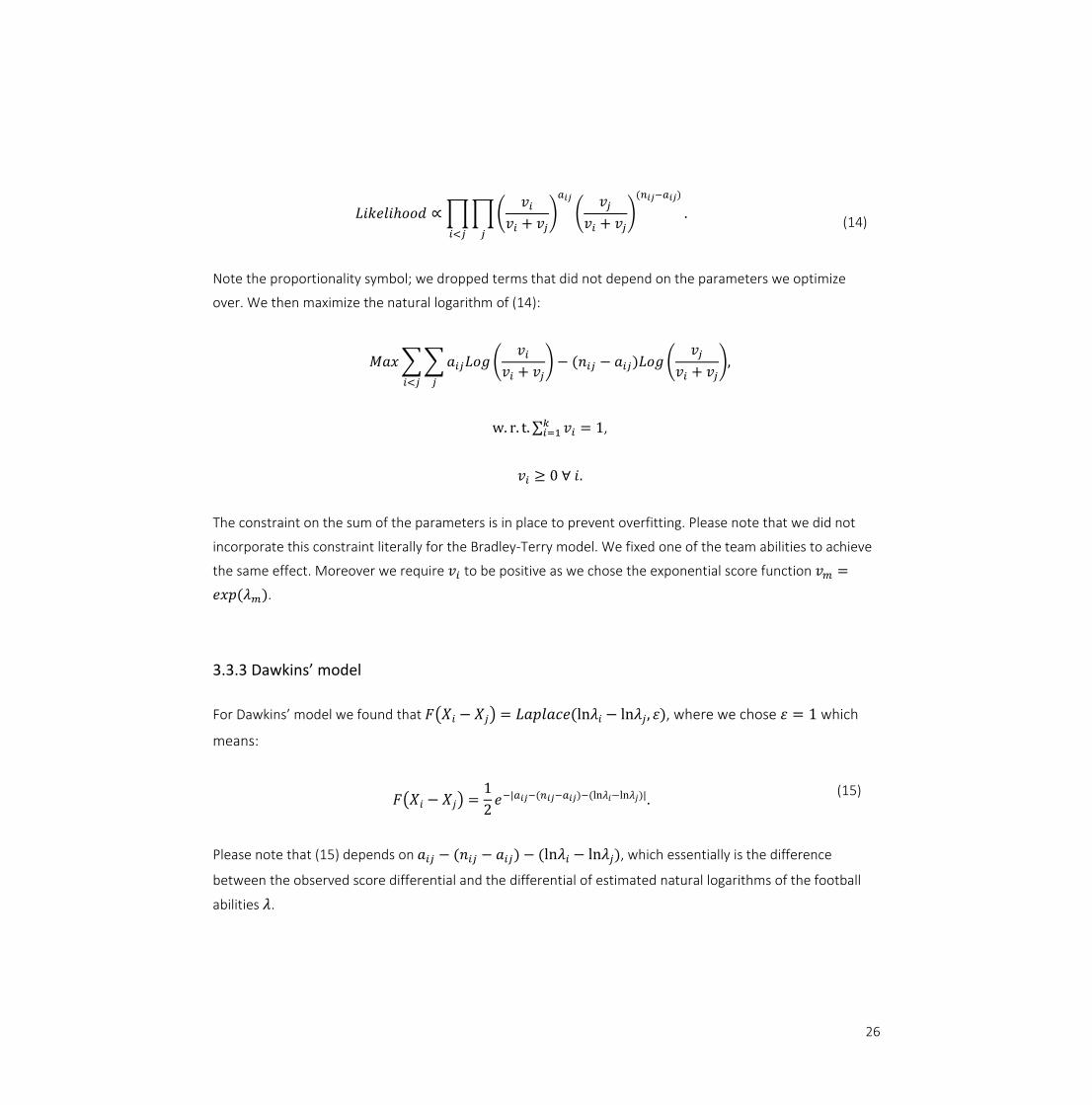
26
𝐿𝑖𝑘𝑒𝑙𝑖ℎ𝑜𝑜𝑑 ∝ ∏ ∏ (𝑣𝑖
𝑣𝑖 + 𝑣𝑗)
𝑎𝑖𝑗
(𝑣𝑗
𝑣𝑖 + 𝑣𝑗)
(𝑛𝑖𝑗−𝑎𝑖𝑗)
.
𝑗𝑖<𝑗
(14)
Note the proportionality symbol; we dropped terms that did not depend on the parameters we optimize
over. We then maximize the natural logarithm of (14):
𝑀𝑎𝑥 ∑ ∑ 𝑎𝑖𝑗𝐿𝑜𝑔 (
𝑣𝑖
𝑣𝑖 + 𝑣𝑗) − (𝑛𝑖𝑗 − 𝑎𝑖𝑗)𝐿𝑜𝑔 (
𝑣𝑗
𝑣𝑖 + 𝑣𝑗)
𝑗𝑖<𝑗
,
w. r. t. ∑ 𝑣𝑖 = 1𝑘𝑖=1 ,
𝑣𝑖 ≥ 0 ∀ 𝑖.
The constraint on the sum of the parameters is in place to prevent overfitting. Please note that we did not
incorporate this constraint literally for the Bradley-Terry model. We fixed one of the team abilities to achieve
the same effect. Moreover we require 𝑣𝑖 to be positive as we chose the exponential score function 𝑣𝑚 =
𝑒𝑥𝑝(𝜆𝑚).
3.3.3 Dawkins’ model
For Dawkins’ model we found that 𝐹(𝑋𝑖 − 𝑋𝑗) = 𝐿𝑎𝑝𝑙𝑎𝑐𝑒(ln𝜆𝑖 − ln𝜆𝑗, 𝜀), where we chose 𝜀 = 1 which
means:
𝐹(𝑋𝑖 − 𝑋𝑗) =1
2𝑒−|𝑎𝑖𝑗−(𝑛𝑖𝑗−𝑎𝑖𝑗)−(ln𝜆𝑖−ln𝜆𝑗)|.
(15)
Please note that (15) depends on 𝑎𝑖𝑗 − (𝑛𝑖𝑗 − 𝑎𝑖𝑗) − (ln𝜆𝑖 − ln𝜆𝑗), which essentially is the difference
between the observed score differential and the differential of estimated natural logarithms of the football
abilities 𝜆.
27
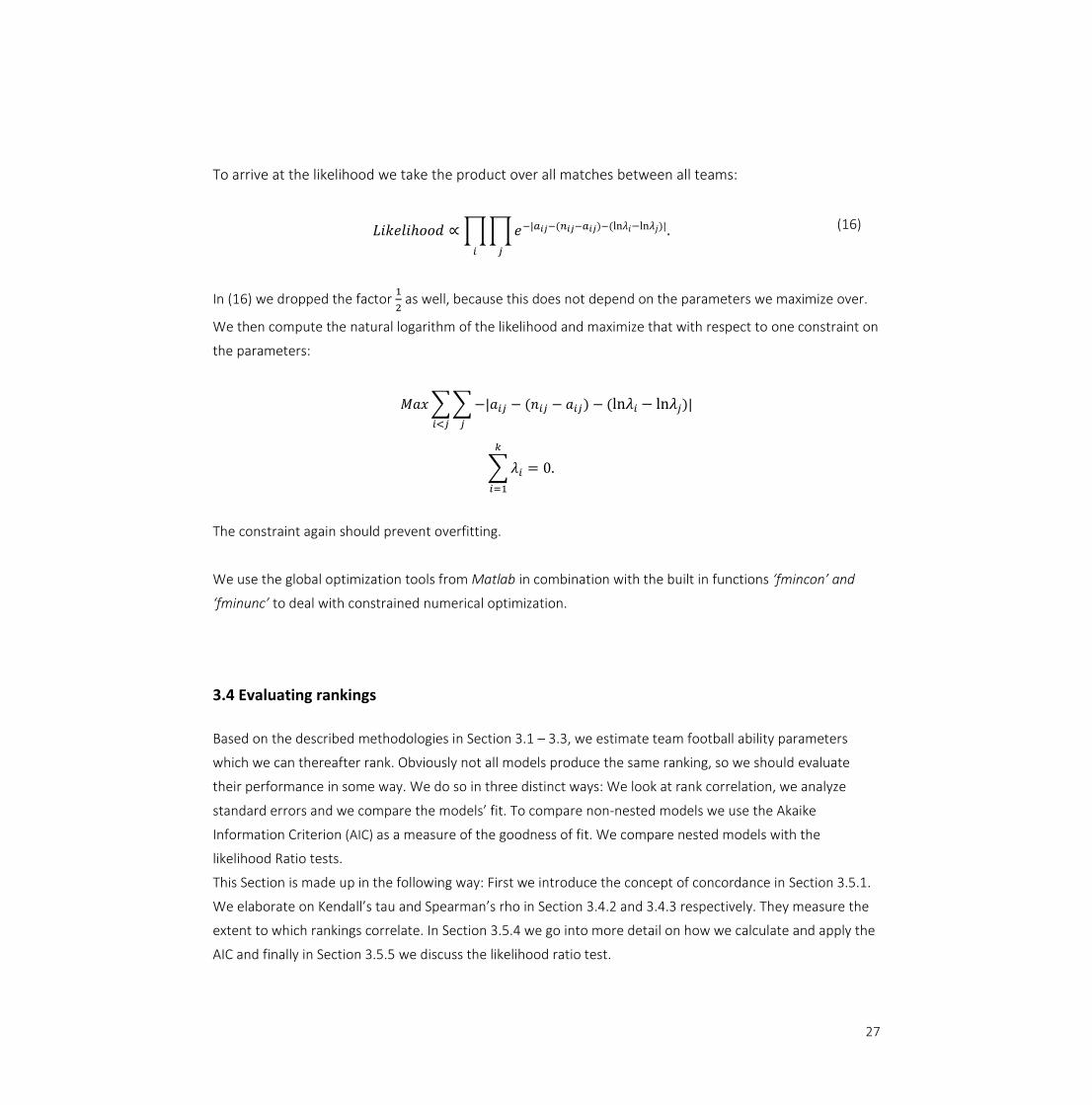
To arrive at the likelihood we take the product over all matches between all teams:
𝐿𝑖𝑘𝑒𝑙𝑖ℎ𝑜𝑜𝑑 ∝ ∏ ∏ 𝑒−|𝑎𝑖𝑗−(𝑛𝑖𝑗−𝑎𝑖𝑗)−(ln𝜆𝑖−ln𝜆𝑗)|
𝑗𝑖
. (16)
In (16) we dropped the factor 1
2 as well, because this does not depend on the parameters we maximize over.
We then compute the natural logarithm of the likelihood and maximize that with respect to one constraint on
the parameters:
𝑀𝑎𝑥 ∑ ∑ −|𝑎𝑖𝑗 − (𝑛𝑖𝑗 − 𝑎𝑖𝑗) − (ln𝜆𝑖 − ln𝜆𝑗)|
𝑗𝑖<𝑗
∑ 𝜆𝑖 = 0
𝑘
𝑖=1
.
The constraint again should prevent overfitting.
We use the global optimization tools from Matlab in combination with the built in functions ‘fmincon’ and
‘fminunc’ to deal with constrained numerical optimization.
3.4 Evaluating rankings
Based on the described methodologies in Section 3.1 – 3.3, we estimate team football ability parameters
which we can thereafter rank. Obviously not all models produce the same ranking, so we should evaluate
their performance in some way. We do so in three distinct ways: We look at rank correlation, we analyze
standard errors and we compare the models’ fit. To compare non-nested models we use the Akaike
Information Criterion (AIC) as a measure of the goodness of fit. We compare nested models with the
likelihood Ratio tests.
This Section is made up in the following way: First we introduce the concept of concordance in Section 3.5.1.
We elaborate on Kendall’s tau and Spearman’s rho in Section 3.4.2 and 3.4.3 respectively. They measure the
extent to which rankings correlate. In Section 3.5.4 we go into more detail on how we calculate and apply the
AIC and finally in Section 3.5.5 we discuss the likelihood ratio test.
28
3.4.1 Concordance
To explain how we compute Kendall's tau and Spearman’s rho, we first have to elaborate on the concept of
concordance and discordance. Say we have a set of 𝑛 observations of the joint random variables 𝑋 and 𝑌.
Moreover, we assume uniqueness of the 𝑥i and 𝑦i. We call pairs of observations concordant if the ranks for
both elements agree and we call pairs of observations discordant if the ranks do not agree:
Concordant: 𝑥i > 𝑥j and 𝑦i > 𝑦j or 𝑥i < 𝑥j and 𝑦i < 𝑦j
Discordant: 𝑥i > 𝑥j and 𝑦i < 𝑦j or if 𝑥i < 𝑥𝑗 and 𝑦i > 𝑦j.
Obviously there is a third category. If 𝑥i = 𝑥j or 𝑦i = 𝑦j, the pair is neither concordant nor discordant.
3.4.2 Kendall’s tau
Kendall’s rank correlation coefficient is developed by Maurice Kendall. With Kendall's tau (𝜏) we measure the
ordinal association between two measured quantities. This is a non-parametric coefficient of correlation on
ranks, or a rank statistic. We use the term ‘correlation’ as a measure of the linear relationship between
covariates. We should rather categorize Kendall's tau as a measure of association because this refers to a
monotone relationship between covariates. We use Kendall’s 𝜏 to distinguish the results of the models from
each other.
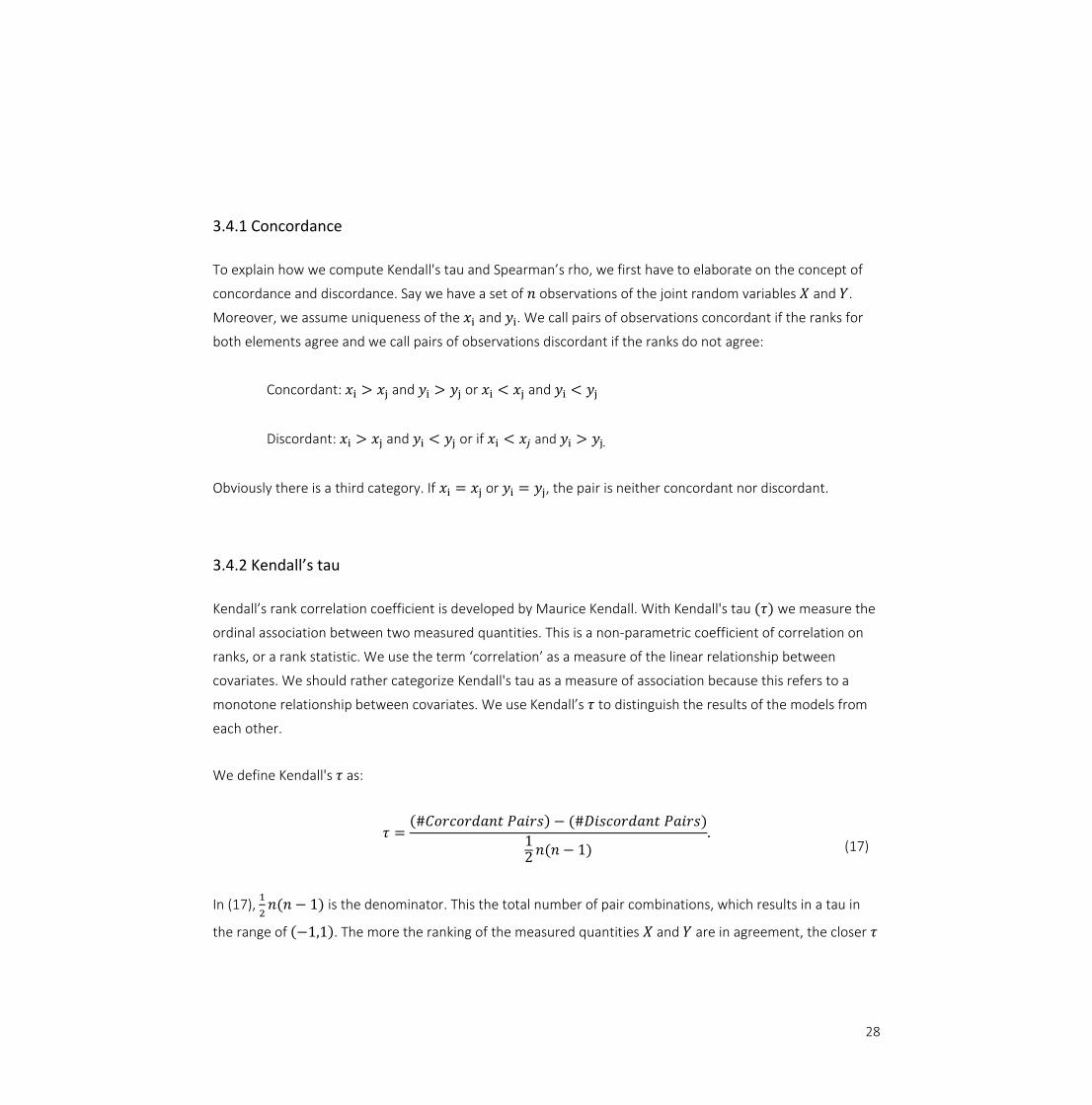
We define Kendall's 𝜏 as:
𝜏 =
(#𝐶𝑜𝑟𝑐𝑜𝑟𝑑𝑎𝑛𝑡 𝑃𝑎𝑖𝑟𝑠) − (#𝐷𝑖𝑠𝑐𝑜𝑟𝑑𝑎𝑛𝑡 𝑃𝑎𝑖𝑟𝑠)
12 𝑛(𝑛 − 1)
.
(17)
In (17), 1
2𝑛(𝑛 − 1) is the denominator. This the total number of pair combinations, which results in a tau in
the range of (−1,1). The more the ranking of the measured quantities 𝑋 and 𝑌 are in agreement, the closer 𝜏
29
is to 1. The opposite is true as well; the more the ranking of the measured quantities 𝑋 and 𝑌 are in
disagreement, the closer 𝜏 is to -1. In the case of independence between the rankings we find 𝜏 = 0.
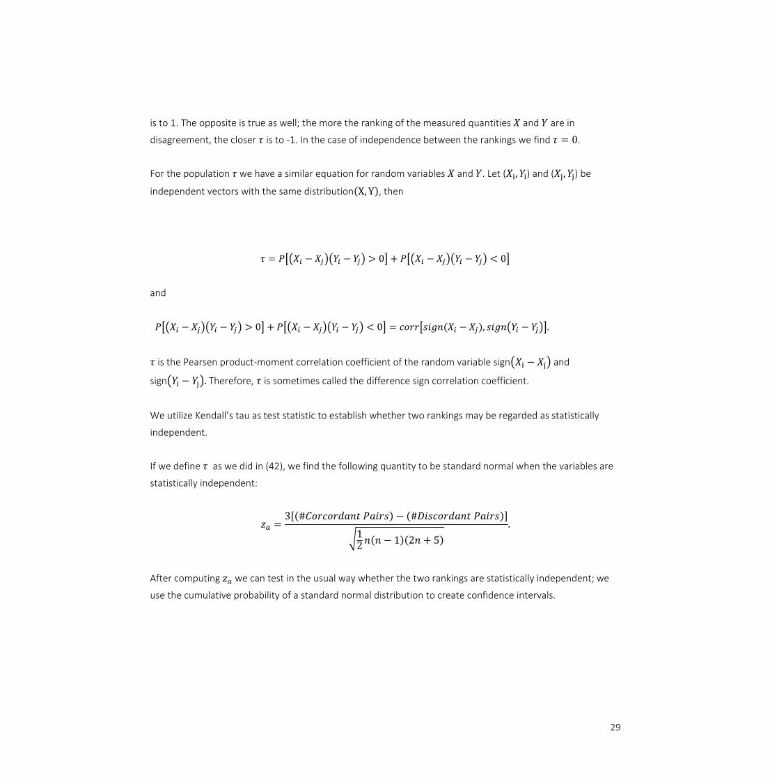
For the population 𝜏 we have a similar equation for random variables 𝑋 and 𝑌. Let (𝑋i, 𝑌i) and (𝑋j, 𝑌j) be
independent vectors with the same distribution(X, Y), then
𝜏 = 𝑃[(𝑋𝑖 − 𝑋𝑗)(𝑌𝑖 − 𝑌𝑗) > 0] + 𝑃[(𝑋𝑖 − 𝑋𝑗)(𝑌𝑖 − 𝑌𝑗) < 0]
and
𝑃[(𝑋𝑖 − 𝑋𝑗)(𝑌𝑖 − 𝑌𝑗) > 0] + 𝑃[(𝑋𝑖 − 𝑋𝑗)(𝑌𝑖 − 𝑌𝑗) < 0] = 𝑐𝑜𝑟𝑟[𝑠𝑖𝑔𝑛(𝑋𝑖 − 𝑋𝑗), 𝑠𝑖𝑔𝑛(𝑌𝑖 − 𝑌𝑗)].
𝜏 is the Pearsen product-moment correlation coefficient of the random variable sign(𝑋i − 𝑋j) and
sign(𝑌i − 𝑌j). Therefore, 𝜏 is sometimes called the difference sign correlation coefficient.
We utilize Kendall’s tau as test statistic to establish whether two rankings may be regarded as statistically
independent.
If we define 𝜏 as we did in (42), we find the following quantity to be standard normal when the variables are
statistically independent:
𝑧𝑎 =
3[(#𝐶𝑜𝑟𝑐𝑜𝑟𝑑𝑎𝑛𝑡 𝑃𝑎𝑖𝑟𝑠) − (#𝐷𝑖𝑠𝑐𝑜𝑟𝑑𝑎𝑛𝑡 𝑃𝑎𝑖𝑟𝑠)]
√12 𝑛(𝑛 − 1)(2𝑛 + 5)
.
After computing 𝑧𝑎 we can test in the usual way whether the two rankings are statistically independent; we
use the cumulative probability of a standard normal distribution to create confidence intervals.
30
3.4.3 Spearman’s rho
Spearman rho (𝜌) is a correlation coefficient developed by the psychologist C. Spearman in 1904. This is a
non-parametric coefficient of correlation on ranks (or a rank statistic) as well. Based on a similar reasoning as
in Section 3.4.2 on Kendall’s tau we should also categorize Spearman’s rho as a measure of association.
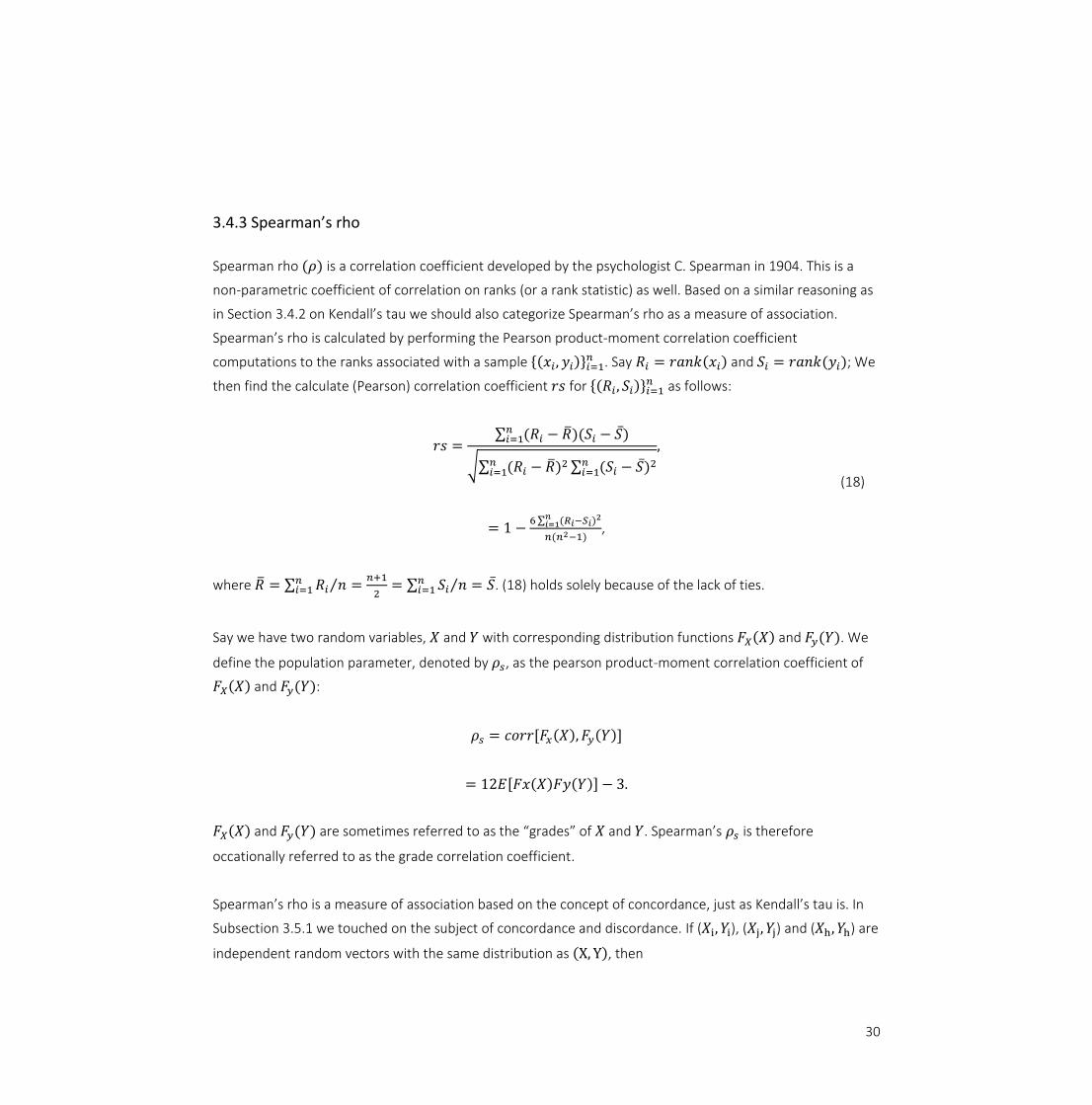
Spearman’s rho is calculated by performing the Pearson product-moment correlation coefficient
computations to the ranks associated with a sample {(𝑥𝑖, 𝑦𝑖)}𝑖=1𝑛 . Say 𝑅𝑖 = 𝑟𝑎𝑛𝑘(𝑥𝑖) and 𝑆𝑖 = 𝑟𝑎𝑛𝑘(𝑦𝑖); We
then find the calculate (Pearson) correlation coefficient 𝑟𝑠 for {(𝑅𝑖 , 𝑆𝑖)}𝑖=1𝑛 as follows:
𝑟𝑠 =
∑ (𝑅𝑖 − �̅�)(𝑆𝑖 − 𝑆̅)𝑛𝑖=1
√∑ (𝑅𝑖 − �̅�)2𝑛𝑖=1 ∑ (𝑆𝑖 − 𝑆̅)2𝑛
𝑖=1
,
= 1 −6 ∑ (𝑅𝑖−𝑆𝑖)2𝑛
𝑖=1
𝑛(𝑛2−1),
(18)
where �̅� = ∑ 𝑅𝑖 𝑛⁄ =𝑛+1
2= ∑ 𝑆𝑖 𝑛⁄𝑛
𝑖=1𝑛𝑖=1 = 𝑆̅. (18) holds solely because of the lack of ties.
Say we have two random variables, 𝑋 and 𝑌 with corresponding distribution functions 𝐹𝑋(𝑋) and 𝐹𝑦(𝑌). We
define the population parameter, denoted by 𝜌𝑠, as the pearson product-moment correlation coefficient of
𝐹𝑋(𝑋) and 𝐹𝑦(𝑌):
𝜌𝑠 = 𝑐𝑜𝑟𝑟[𝐹𝑥(𝑋), 𝐹𝑦(𝑌)]
= 12𝐸[𝐹𝑥(𝑋)𝐹𝑦(𝑌)] − 3.
𝐹𝑋(𝑋) and 𝐹𝑦(𝑌) are sometimes referred to as the “grades” of 𝑋 and 𝑌. Spearman’s 𝜌𝑠 is therefore
occationally referred to as the grade correlation coefficient.
Spearman’s rho is a measure of association based on the concept of concordance, just as Kendall’s tau is. In
Subsection 3.5.1 we touched on the subject of concordance and discordance. If (𝑋i, 𝑌i), (𝑋j, 𝑌j) and (𝑋h, 𝑌h) are
independent random vectors with the same distribution as (X, Y), then
31
𝜌𝑠 = 3𝑃[(𝑋i − 𝑋j)(𝑌i − 𝑌h) > 0] − 3𝑃[(𝑋i − 𝑋j)(𝑌i − 𝑌h) < 0]. (19)
That is; the difference between the probabilities of concordance and discordance between the random
vectors (𝑋i, 𝑌𝑖) and (𝑋𝑗, 𝑌ℎ) is proportional to 𝜌𝑠. Obviously we can swap (𝑋𝑗, 𝑌ℎ) for (𝑋ℎ , 𝑌𝑗) in (19).
As Spearman’s rho is nothing else than Pearson’s linear correlation we can use a 𝑡-test for its significance. We
should however perform a transformation on 𝑟 in the following way:
𝑡 = 𝑟√𝑛 − 2
1 − 𝑟2.
This statistic is approximately distributed as a Student’s 𝑡-distribution with n-2 degrees of freedom under the
null hypothesis.
3.4.4 Akaike information criterion
We measure the goodness of fit with the Akaike information criterion (AIC). When adding parameters to
models, the model never gets worse in terms of fitting the training sample. With every extra parameter we
introduce the model loses generalization power. Out of sample estimation might perform worse with the
introduction of extra parameters. Moreover, more complex models are more difficult to interpret. AIC offers
a relative estimate of the information lost when a given model is used to represent the process that
generates the data. In doing so, it deals with the trade-off between the goodness of fit of the model and the
complexity of the model. AIC does so by introducing a penalty term for the number of parameters in the
model.
To compare nested models we use the likelihood ratio test as well. For non-nested models we cannot do
likelihood ratio tests as these are restricted to nested models. Therefore, we use AIC to compare non-nested
models.
AIC measures the fit of a model relative to other models for a given dataset. While this does not quantify the
absolute fit for a given model, it does provide a means for model selection. This means there is no concrete
test in which we reject or accept some null hypothesis.
32
Let 𝐿 denote the maximum likelihood value under some model and let 𝑘 denote the number of estimated
parameters in the model. AIC then has the following equation:
𝐴𝐼𝐶 = 2𝑘 − 2 log(𝐿).
The model with the highest absolute AIC value is favored.
3.4.5 Likelihood ratio test
The likelihood ratio test is used to compare nested models. In our case the models without a home parameter
are nested within models with a home parameter. This is quite straightforward as one can simply impose the
restriction that the home parameter is equal to zero. The intuition is that we calculate the ratio between the
model with the restriction and without the restriction. Based on this ratio we can perform tests on whether or
not the difference in likelihood is significant.
Let 𝐿1 be the maximum value of the likelihood of the data without the additional restriction. In other words,
𝐿1 is the likelihood of the data with all the parameters unrestricted and maximum likelihood estimates
substituted for these parameters. Let 𝐿0 be the maximum value of the likelihood when the parameters are
restricted (and reduced in number) based on the assumption. Assume 𝑘 parameters were lost (so 𝐿0 has 𝑘
less parameters than 𝐿1).
We compute the ratio 𝐿0
𝐿1, which should be between 0 and 1. The less likely the assumption is, the smaller
𝐿0
𝐿1 will be. We calculate −2 𝐿𝑛(
𝐿0
𝐿1) , which is distributed as 𝜒2(𝑘) where 𝑘 is the number of restrictions we
impose.
In our case, 𝐿1 is the likelihood of the data with the model with the home parameter and 𝐿0 is the likelihood
of the data without the home parameter. This means we calculate −2 𝐿𝑛(𝐿0
𝐿1) and compare its value to a
𝜒2(1) cumulative distribution function.
33
4. Results
This Section contains the findings of this research. Section 4.1 is aimed at the comparison between the
models by Thurstone, Bradley-Terry and Dawkins. In Section 4.2 we discuss the model with a home
parameter. We use Kendall’s tau, Spearman’s rho and Akaike Information Criterion (AIC) as evaluation criteria
and perform the appropriate tests. Finally, 4.3 contains the results of the comparison of the simple model to
the model with a home parameter through the likelihood ratio tests.
4.1 Simple Model
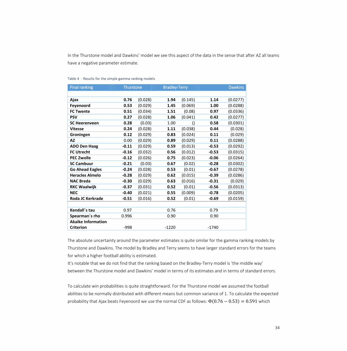
The first model we consider is the model where we estimate the team’s football ability with the simple
model: 𝑋𝑖 = 𝜆𝑖 + 𝜀. Table 4 shows the estimates for 𝜆𝑖 based on the different models. Please note that SC
Heerenveen is the reference category for the Bradley-Terry model.
As expected, the three gamma ranking models show a similar ranking in terms of their point estimate. The
final three rows in Table 4 show Kendall’s tau, Spearman’s rho and the AIC values for these three models.
Kendall’s tau and Spearman’s rho paint the same picture: Thurstone’s model, the gamma ranking model with
the shape parameter going to infinity, is closest to the real ranking in terms of the distance measured by
Kendall’s tau. Dawkins’ model, with a shape parameter going to zero, takes a second place and the model
with a shape parameter of 1, the Bradley-Terry is model third. Bradley-Terry’s model and Dawkins’ model are
not relatively just far apart from the real ranking when considering their Kendall’s tau values are 0.76 and
0.79 respectively. This is in contrast to the value corresponding to the Thurstone model, which is 0.97. This is
once more underlined by the Spearman’s rho values that also find the gamma ranking model with a relatively
large shape parameter (𝑟 → ∞), Thurstone’s model, to be closest to the real ranking. Moreover, the distance
measured by Spearman´s rho between Bradley and Terry’s model and Dawkins’ model is similar with a value
of 0.90.
The parameter estimates are all significantly different from zero (marked bold in Table 4). The reference
category (SC Heerenveen) in the Bradley-Terry model does not have an estimated standard error.
The goal deficit is only positive from Ajax to AZ as is shown in the final column in Table 3 in the data Section.
We estimated these models on the goal deficit data instead of on the match outcome (win, draw, loss) data.
34
In the Thurstone model and Dawkins’ model we see this aspect of the data in the sense that after AZ all teams
have a negative parameter estimate.
Table 4 - Results for the simple gamma ranking models
The absolute uncertainty around the parameter estimates is quite similar for the gamma ranking models by
Thurstone and Dawkins. The model by Bradley and Terry seems to have larger standard errors for the teams
for which a higher football ability is estimated.
It’s notable that we do not find that the ranking based on the Bradley-Terry model is ‘the middle way’
between the Thurstone model and Dawkins’ model in terms of its estimates and in terms of standard errors.
To calculate win probabilities is quite straightforward. For the Thurstone model we assumed the football
abilities to be normally distributed with different means but common variance of 1. To calculate the expected
probability that Ajax beats Feyenoord we use the normal CDF as follows: Ф(0.76 − 0.53) = 0.591 which
Final ranking Thurstone Bradley-Terry Dawkins
Ajax 0.76 (0.028) 1.94 (0.145) 1.14 (0.0277)
Feyenoord 0.53 (0.029) 1.45 (0.069) 1.00 (0.0288)
FC Twente 0.51 (0.034) 1.51 (0.08) 0.97 (0.0336)
PSV 0.27 (0.028) 1.06 (0.041) 0.42 (0.0277)
SC Heerenveen 0.28 (0.03) 1.00 () 0.58 (0.0301)
Vitesse 0.24 (0.028) 1.11 (0.038) 0.44 (0.028)
Groningen 0.12 (0.029) 0.83 (0.024) 0.11 (0.029)
AZ 0.00 (0.029) 0.89 (0.029) 0.11 (0.0288)
ADO Den Haag -0.11 (0.029) 0.59 (0.013) -0.53 (0.0292)
FC Utrecht -0.16 (0.032) 0.56 (0.012) -0.53 (0.0315)
PEC Zwolle -0.12 (0.026) 0.75 (0.023) -0.06 (0.0264)
SC Cambuur -0.21 (0.03) 0.67 (0.02) -0.28 (0.0302)
Go Ahead Eagles -0.24 (0.028) 0.53 (0.01) -0.67 (0.0278)
Heracles Almelo -0.28 (0.029) 0.62 (0.015) -0.39 (0.0286)
NAC Breda -0.30 (0.029) 0.63 (0.016) -0.31 (0.029)
RKC Waalwijk -0.37 (0.031) 0.52 (0.01) -0.56 (0.0313)
NEC -0.40 (0.021) 0.55 (0.009) -0.78 (0.0205)
Roda JC Kerkrade -0.51 (0.016) 0.52 (0.01) -0.69 (0.0159)
Kendall´s tau 0.97 0.76 0.79
Spearman´s rho 0.996 0.90 0.90
Akaike Information Criterion -998 -1220 -1740
35
means the expected probability Ajax beats Feyenoord is 59.1 %. Similarly for the Bradley-Terry model we
compute the expected probability that Ajax beats Feyenoord as 𝑒1.94
(𝑒1.94+𝑒1.45)= 0.6201 which is 62.01%. For
the Dawkins model we use the Laplace CDF: 1
2+
1
2𝑠𝑔𝑛(1.14 − 1)(1 − 𝑒(−|1.14−1|)) = 0.5653 or 56.53%. Note
that the match played in Amsterdam ended in 2-1 just as the match played in Rotterdam ended in 2-1. This
means the goal deficit over these matches is 0. Clearly these estimates are highly similar.
Note that the underlying distributions for the football ability in Thurstone’s Case V model is the normal
distribution, while Luce’s choice axiom implies Gumbel football abilities and Dawkins’ model corresponds to
exponential football abilities. These models imply normally distributed, logistically distributed and Laplace
distributed match outcomes.
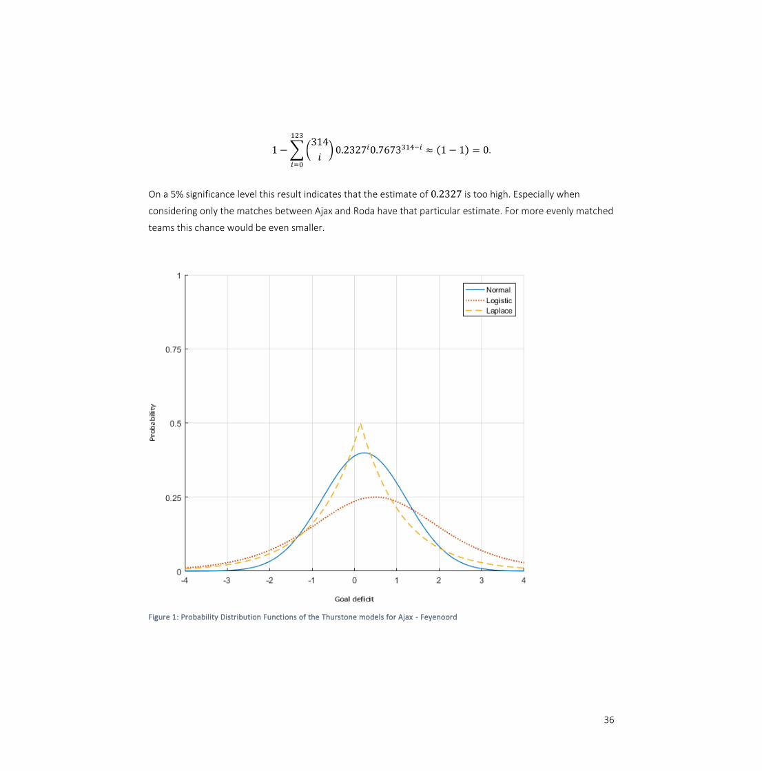
Figure 1 shows the simulated distributions for the outcome of the match Ajax – Feyenoord according to these
three distributions. It’s evident that these distributions are located at 0.76 − 0.53 = 0.23, 1.94 − 1.45 =
0.49 and 1.14 − 1 = 0.14 for the normal, logistic and exponential distributions respectively. Moreover, all
three distributions are symmetrical. In our context this means negative and positive deviations from the point
estimate have the same implication for the probabilities of such outcomes.
Moreover, we see that the logistic distribution and the Laplace distribution have fatter tails. These
distributions are better equipped to deal with data with more outliers than in the normal case. Based on the
simulated densities we calculate the corresponding kurtoses to show this: The kurtoses in our simulations are
3.0020, 4.197 and 5.9943 for the normal, logistic and Laplace model respectively. In this sense the logistic
model is in between the normal model and the Laplace model. This finding extends to cases in which we
compare more than two items at a time.
As additional proof of the fact that the normal distribution cannot cope with the fat tails in the data in
comparison to the logistic and Laplace distribution, we calculate binomial cumulative probabilities and
perform the appropriate tests.
We empirically observe 123 out of 314 matches ending with a goal deficit of at least 2. This is a proportion of
0.3917. We calculate the probability of Ajax beating Roda JC Kerkrade with at least 2 goals, because Ajax and
Roda JC Kerkrade have the highest and lowest estimated football abilities respectively. Any binomial
cumulative probability based on this probability should be considered an upper limit. The outcome of the
match Ajax – Roda is distributed with a variance of 1 around the location, 0.76 − −0.51 = 1.27. The
probability is then: 1 − Ф(2 − 1.27) ≈ 0.2327. The probability of observing more than 123 of such match
results is:
36
1 − ∑ (314
𝑖) 0.2327𝑖0.7673314−𝑖
123
𝑖=0
≈ (1 − 1) = 0.
On a 5% significance level this result indicates that the estimate of 0.2327 is too high. Especially when
considering only the matches between Ajax and Roda have that particular estimate. For more evenly matched
teams this chance would be even smaller.
Figure 1: Probability Distribution Functions of the Thurstone models for Ajax - Feyenoord
37
Following a similar reasoning for the other models we find the probability of Ajax beating Roda with at least a
2 goal deficit to be𝑒1.94
(𝑒1.94−𝑒0.52)= 0.8053 and
1
2+
1
2𝑠𝑔𝑛(2 − 1.14 − 0.69)(1 − 𝑒(−|2−1.14−0.69|)) = 0.5782 for
the logistic and Laplace models.
The AIC values back up the claim that the logistic distribution and Laplace distribution are better able to deal
with the fatter tails in the data. The model by Dawkins has the highest absolute value for AIC, the measure of
goodness of fit. Bradley-Terry is second in this regard, while Thurstone is third. The corresponding values are -
998, -1220 and -1740, respectively. Based on these findings, Dawkins’ model seems to be the best fit.
We believe this is due to the fact that the Laplace distribution combines fat tails with a narrow peak.
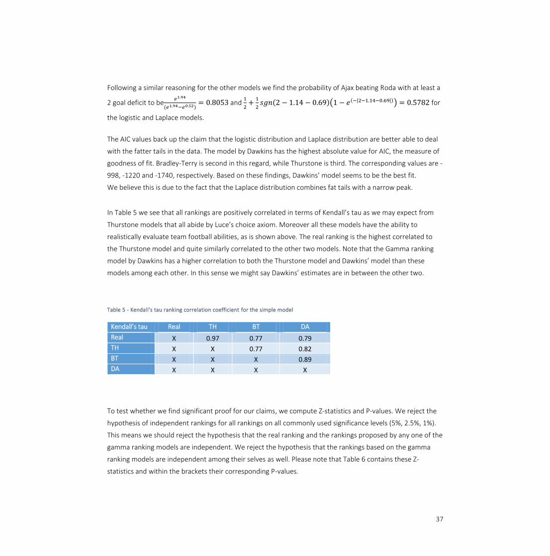
In Table 5 we see that all rankings are positively correlated in terms of Kendall’s tau as we may expect from
Thurstone models that all abide by Luce’s choice axiom. Moreover all these models have the ability to
realistically evaluate team football abilities, as is shown above. The real ranking is the highest correlated to
the Thurstone model and quite similarly correlated to the other two models. Note that the Gamma ranking
model by Dawkins has a higher correlation to both the Thurstone model and Dawkins’ model than these
models among each other. In this sense we might say Dawkins’ estimates are in between the other two.
Table 5 - Kendall's tau ranking correlation coefficient for the simple model
To test whether we find significant proof for our claims, we compute Z-statistics and P-values. We reject the
hypothesis of independent rankings for all rankings on all commonly used significance levels (5%, 2.5%, 1%).
This means we should reject the hypothesis that the real ranking and the rankings proposed by any one of the
gamma ranking models are independent. We reject the hypothesis that the rankings based on the gamma
ranking models are independent among their selves as well. Please note that Table 6 contains these Z-
statistics and within the brackets their corresponding P-values.
Kendall’s tau Real TH BT DA
Real X 0.97 0.77 0.79
TH X X 0.77 0.82
BT X X X 0.89
DA X X X X
38
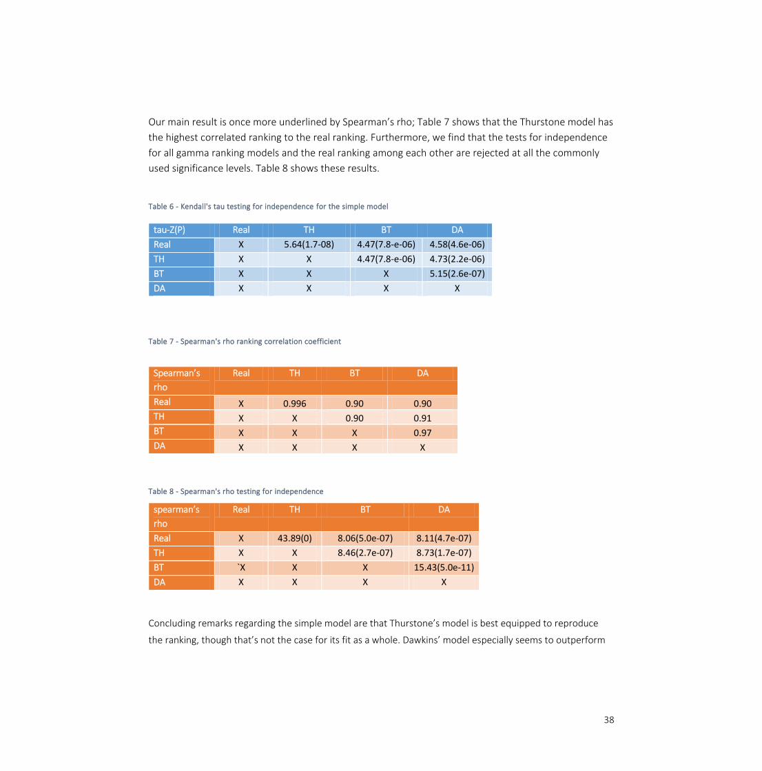
Our main result is once more underlined by Spearman’s rho; Table 7 shows that the Thurstone model has
the highest correlated ranking to the real ranking. Furthermore, we find that the tests for independence
for all gamma ranking models and the real ranking among each other are rejected at all the commonly
used significance levels. Table 8 shows these results.
Table 6 - Kendall's tau testing for independence for the simple model
Table 7 - Spearman's rho ranking correlation coefficient
Table 8 - Spearman's rho testing for independence
Concluding remarks regarding the simple model are that Thurstone’s model is best equipped to reproduce
the ranking, though that’s not the case for its fit as a whole. Dawkins’ model especially seems to outperform
tau-Z(P) Real TH BT DA
Real X 5.64(1.7-08) 4.47(7.8-e-06) 4.58(4.6e-06)
TH X X 4.47(7.8-e-06) 4.73(2.2e-06)
BT X X X 5.15(2.6e-07)
DA X X X X
Spearman’s
rho
Real TH BT DA
Real X 0.996 0.90 0.90
TH X X 0.90 0.91
BT X X X 0.97
DA X X X X
spearman’s
rho
Real TH BT DA
Real X 43.89(0) 8.06(5.0e-07) 8.11(4.7e-07)
TH X X 8.46(2.7e-07) 8.73(1.7e-07)
BT `X X X 15.43(5.0e-11)
DA X X X X

39
Thurston’s model and Bradley-Terry’s model in that regard because of its ability to model fat tails as well as
sharp peaks.
4.2 Model with home parameter
While our measures of association agreed on the fact that the rankings based on the simple gamma ranking
models were relatively close to the real ranking, we believe a home parameter would be a great addition. This
was supported by the fact that we empirically found a home advantage in Section 2. We estimated the
model: 𝑋𝑖 = 𝜆𝑖 + 𝐻𝑜𝑚𝑒 + 𝜀.
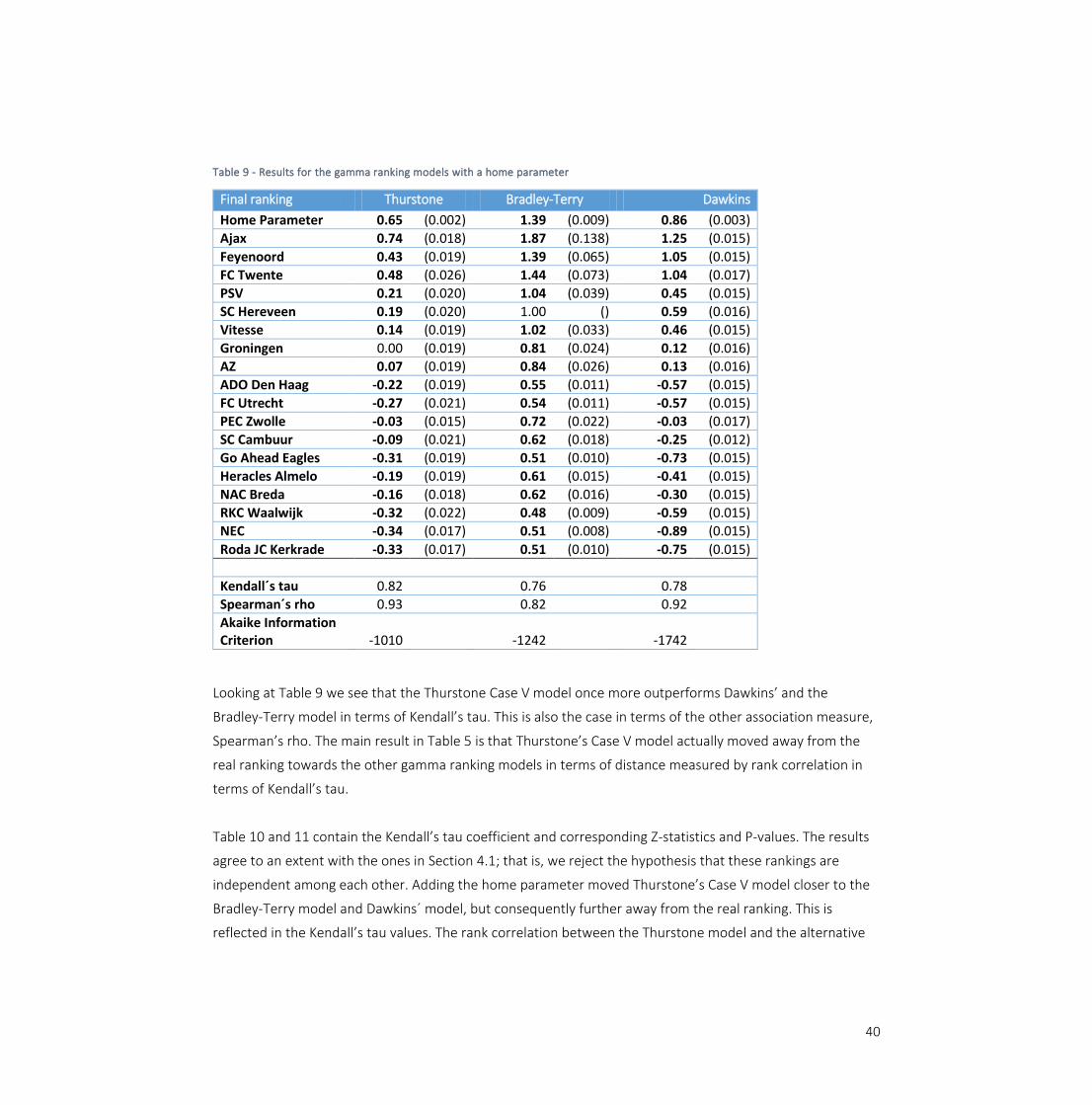
Table 9 shows the results for the gamma ranking models based on the model with a home parameter. Table 9
is built up in the same fashion as Table 4, except for the fact that the first row contains the home parameter
estimates.
We used an additive model, in the sense that the team football ability at home is simply calculated by adding
the home parameter to the strength parameter. A fairly obvious but important observation is that the home
parameter is positive in all models, which means we find support for a home advantage in our model. More
specifically, the advantage of playing at home is larger than the football ability of quite a lot of teams. For
Thurstone’s model and the Bradley-Terry model only Ajax’ estimated football ability is larger than the home
advantage. Bradley-Terry’s model has a relatively small home parameter.
The model by Dawkins has the highest absolute value for AIC, the measure of goodness of fit. Bradley-Terry is
second in this regard, while Thurstone is third. This is in agreement with our findings from the simple model.
The corresponding values are -1010, -1242, and -1742 respectively. Based on these findings Dawkins’ model
seems to be the best fit.
We estimate the probability of Ajax to beat Feyenoord when playing at home to be Ф(0.74 + 0.65 − 0.43) =
0.8365, which is 83.15%. For the Bradley-Terry model we find that same probability as follows:
𝑒1.87+1.39
(𝑒1.87+1.39+𝑒1.39)= 0.8665 or 86.65%.
With the Dawkins model we use the Laplace CDF: 1
2+
1
2𝑠𝑔𝑛(1.25 + 0.86 − 1.05)(1 − 𝑒(−|1.25+0.86−1.05|)) =
0.8268 or 82.68%.
40
Table 9 - Results for the gamma ranking models with a home parameter
Looking at Table 9 we see that the Thurstone Case V model once more outperforms Dawkins’ and the
Bradley-Terry model in terms of Kendall’s tau. This is also the case in terms of the other association measure,
Spearman’s rho. The main result in Table 5 is that Thurstone’s Case V model actually moved away from the
real ranking towards the other gamma ranking models in terms of distance measured by rank correlation in
terms of Kendall’s tau.
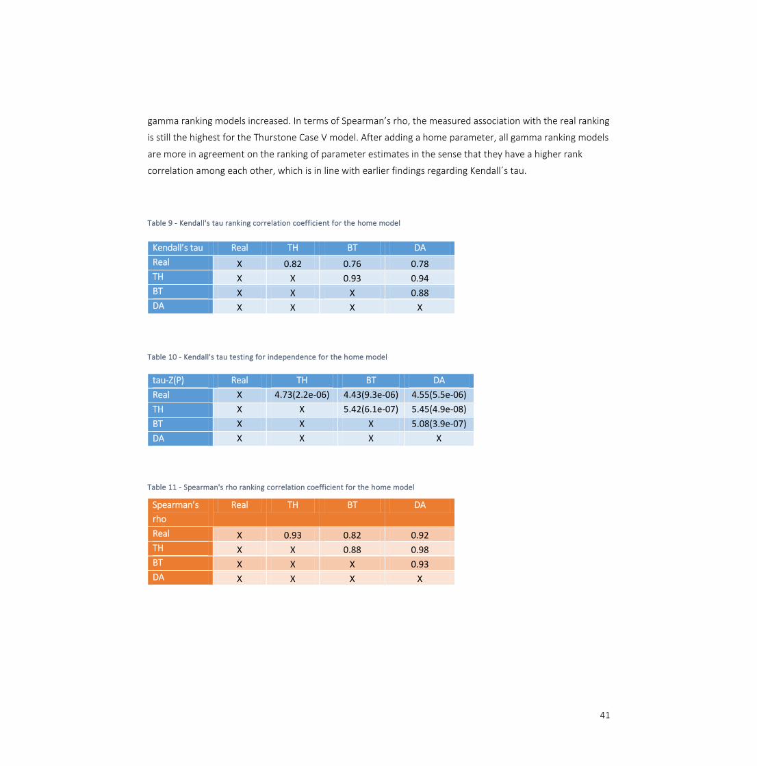
Table 10 and 11 contain the Kendall’s tau coefficient and corresponding Z-statistics and P-values. The results
agree to an extent with the ones in Section 4.1; that is, we reject the hypothesis that these rankings are
independent among each other. Adding the home parameter moved Thurstone’s Case V model closer to the
Bradley-Terry model and Dawkins´ model, but consequently further away from the real ranking. This is
reflected in the Kendall’s tau values. The rank correlation between the Thurstone model and the alternative
Final ranking Thurstone Bradley-Terry Dawkins
Home Parameter 0.65 (0.002) 1.39 (0.009) 0.86 (0.003)
Ajax 0.74 (0.018) 1.87 (0.138) 1.25 (0.015)
Feyenoord 0.43 (0.019) 1.39 (0.065) 1.05 (0.015)
FC Twente 0.48 (0.026) 1.44 (0.073) 1.04 (0.017)
PSV 0.21 (0.020) 1.04 (0.039) 0.45 (0.015)
SC Hereveen 0.19 (0.020) 1.00 () 0.59 (0.016)
Vitesse 0.14 (0.019) 1.02 (0.033) 0.46 (0.015)
Groningen 0.00 (0.019) 0.81 (0.024) 0.12 (0.016)
AZ 0.07 (0.019) 0.84 (0.026) 0.13 (0.016)
ADO Den Haag -0.22 (0.019) 0.55 (0.011) -0.57 (0.015)
FC Utrecht -0.27 (0.021) 0.54 (0.011) -0.57 (0.015)
PEC Zwolle -0.03 (0.015) 0.72 (0.022) -0.03 (0.017)
SC Cambuur -0.09 (0.021) 0.62 (0.018) -0.25 (0.012)
Go Ahead Eagles -0.31 (0.019) 0.51 (0.010) -0.73 (0.015)
Heracles Almelo -0.19 (0.019) 0.61 (0.015) -0.41 (0.015)
NAC Breda -0.16 (0.018) 0.62 (0.016) -0.30 (0.015)
RKC Waalwijk -0.32 (0.022) 0.48 (0.009) -0.59 (0.015)
NEC -0.34 (0.017) 0.51 (0.008) -0.89 (0.015)
Roda JC Kerkrade -0.33 (0.017) 0.51 (0.010) -0.75 (0.015)
Kendall´s tau 0.82 0.76 0.78
Spearman´s rho 0.93 0.82 0.92
Akaike Information Criterion -1010 -1242 -1742
41
gamma ranking models increased. In terms of Spearman’s rho, the measured association with the real ranking
is still the highest for the Thurstone Case V model. After adding a home parameter, all gamma ranking models
are more in agreement on the ranking of parameter estimates in the sense that they have a higher rank
correlation among each other, which is in line with earlier findings regarding Kendall´s tau.
Table 9 - Kendall's tau ranking correlation coefficient for the home model
Table 10 - Kendall's tau testing for independence for the home model
Table 11 - Spearman's rho ranking correlation coefficient for the home model
Kendall’s tau Real TH BT DA
Real X 0.82 0.76 0.78
TH X X 0.93 0.94
BT X X X 0.88
DA X X X X
tau-Z(P) Real TH BT DA
Real X 4.73(2.2e-06) 4.43(9.3e-06) 4.55(5.5e-06)
TH X X 5.42(6.1e-07) 5.45(4.9e-08)
BT X X X 5.08(3.9e-07)
DA X X X X
Spearman’s
rho
Real TH BT DA
Real X 0.93 0.82 0.92
TH X X 0.88 0.98
BT X X X 0.93
DA X X X X

42
Table 12 - Testing for independence for Spearman's rho for the home model
4.3 Nested model comparisons
In Section 4.1 we compared the non-nested models. To compare the models based on their fit we compare
the models´ standard errors and perform the likelihood ratio test in this Section.
Generally speaking, the gamma ranking models with a home parameter have smaller standard errors than the
ones without a home parameter (please note that we are comparing Thurstone Case V models among each
other, Bradley-Terry models among each other and Dawkins’ models among each other). This means we
estimate our parameters, the football abilities, more accurately after we add a home parameter. Moreover
the home parameter was significantly different from 0. Based on these findings we conclude that the real
ranking obviously is influenced by a home effect, which causes Thurstone’s model to have a lower ranking
correlation after introducing a home effect in our model. This separates a home advantage effect from
football ability, which clearly is not the case for the real rankings. When attempting to mimic the real ranking
one should not add a home effect, however when attempting to model the latent football abilities, one
definitely should add a home advantage effect.
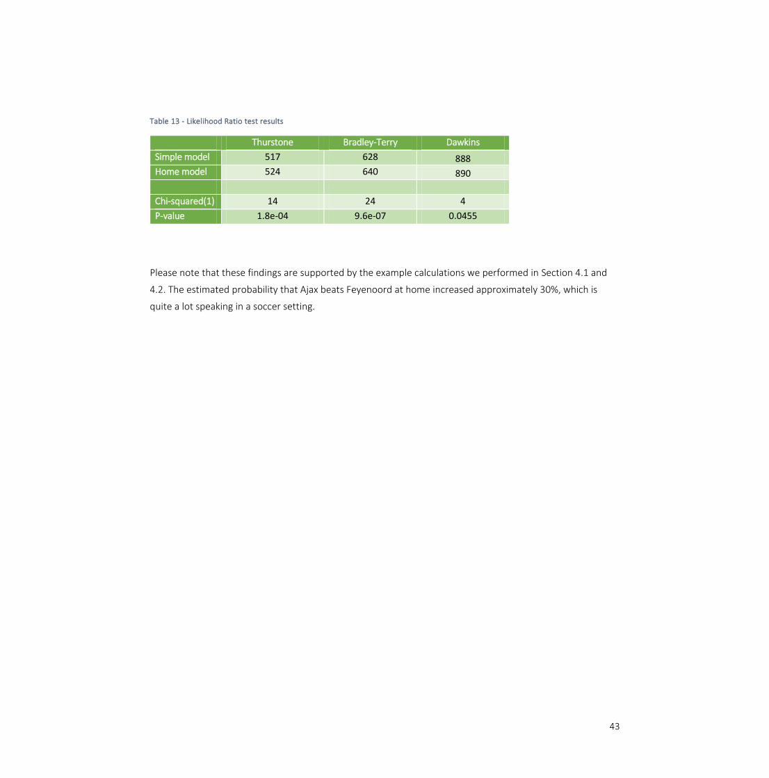
To test whether or not we find similar evidence in terms of likelihood, we show results of the likelihood ratio
tests in Table 14. All three gamma ranking models agree on the results. We reject the hypothesis that the
model with additional restriction perform just as well as the model without the restriction on all commonly
used significance levels. This means we conclude that the increase in likelihood based on our data is
significant on the 5% significance level and that we reject the hypothesis that both models are just as likely
based on the data.
Spearman’s
rho
Real TH BT DA
Real X 40.88(0) 7.35(1.6e-07) 8.29(3.5e-07)
TH X X 8.23(3.8e-07) 9.38(6.7e-8)
BT X X X 14.82(9.1e-11)
DA X X X X
43
Table 13 - Likelihood Ratio test results
Please note that these findings are supported by the example calculations we performed in Section 4.1 and
4.2. The estimated probability that Ajax beats Feyenoord at home increased approximately 30%, which is
quite a lot speaking in a soccer setting.
Thurstone Bradley-Terry Dawkins
Simple model 517 628 888
Home model 524 640 890
Chi-squared(1) 14 24 4
P-value 1.8e-04 9.6e-07 0.0455

44
Conclusion
In this research we investigate which of the gamma ranking models, that are closely related to Luce´s choice
axiom, measure latent football abilities most accurately when modelling football matches as discriminal
Thurstone processes as described by the law of comparative judgment; we considered Thurstone’s Case V
model, the Bradley-Terry model and Dawkins’ model and measured their distance to the real ranking by
Kendall’s tau. Furthermore, we compared their goodness of fit by computing AIC values. We show that the
parameters estimates by Thurstone’s model, the normal model, are closest to the real Eredivisie ranking in
terms of ranking correlation. Moreover, all three gamma ranking models are well equipped to model football
abilities, because of similarities in terms of their difference distribution. In terms of the goodness of fit
Dawkins’ model, the Laplace model, seems to outperform the other models because of its ability to model fat
tails as well as a sharp peak. Thurstone’s model lacks the first of those abilities and the model by Bradley and
Terry, the logistic model, lacks the second. Additionally, our findings suggest that adding a home advantage
effect is a valuable extension to the gamma ranking models in the sense that the football abilities are
estimated more efficiently and the likelihood increases significantly when introducing a home effect.
Future work
Further research could investigate how the skill of the individual team players or the number of matches they
have played together, or synergy if you will, affect the team skill pre-game. Other extensions include team
experience or even dependence among consecutive games. In (Cattelan, 2009) it is shown how to deal with
the dependence among the performances of a team. To incorporate these effects one should collect (or
construct) the appropriate data and reformulate the likelihoods we specified in Section 3.3. Finally team
dependent home parameters can also be investigated. This essentially comes down to modelling the same
team, playing at home and playing away, as two separate teams. In our research this has no use as we will get
two different parameters per team and therefore ranking a team football ability will not make sense
intuitively.
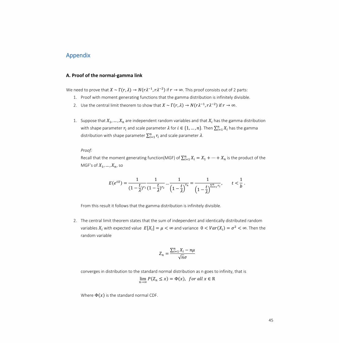
45
Appendix
A. Proof of the normal-gamma link
We need to prove that 𝑋 ~ Γ(𝑟, 𝜆) → 𝑁(𝑟𝜆−1, 𝑟𝜆−2) if 𝑟 → ∞. This proof consists out of 2 parts:
1. Proof with moment generating functions that the gamma distribution is infinitely divisible.
2. Use the central limit theorem to show that 𝑋 ~ Γ(𝑟, 𝜆) → 𝑁(𝑟𝜆−1, 𝑟𝜆−2) if 𝑟 → ∞.
1. Suppose that 𝑋1, … , 𝑋𝑛 are independent random variables and that 𝑋𝑖 has the gamma distribution
with shape parameter 𝑟𝑖 and scale parameter 𝜆 for 𝑖 ∈ {1, … , 𝑛}. Then ∑ 𝑋𝑖𝑛𝑖=1 has the gamma
distribution with shape parameter ∑ 𝑟𝑖𝑛𝑖=1 and scale parameter 𝜆.
Proof:
Recall that the moment generating function(MGF) of ∑ 𝑋𝑖𝑛𝑖=1 = 𝑋1 + ⋯ + 𝑋𝑛 is the product of the
MGF’s of 𝑋1, … , 𝑋𝑛, so
𝐸(𝑒𝑡𝑋) =1
(1 −𝑡𝜆
)𝑟𝑖
1
(1 −𝑡𝜆
)𝑟2
…1
(1 −𝑡𝜆)
𝑟𝑛=
1
(1 −𝑡𝜆)
∑ 𝑟𝑖𝑛𝑖=1
, 𝑡 <1
𝑏 .
From this result it follows that the gamma distribution is infinitely divisible.
2. The central limit theorem states that the sum of independent and identically distributed random
variables 𝑋𝑖 with expected value 𝐸[𝑋𝑖] = 𝜇 < ∞ and variance 0 < 𝑉𝑎𝑟(𝑋𝑖) = 𝜎2 < ∞. Then the
random variable
𝑍𝑛 =∑ 𝑋𝑖
𝑛𝑖=1 − 𝑛𝜇
√𝑛𝜎
converges in distribution to the standard normal distribution as n goes to infinity, that is
lim𝑛→∞
𝑃(𝑍𝑛 ≤ 𝑥) = Φ(𝑥), 𝑓𝑜𝑟 𝑎𝑙𝑙 𝑥 ∈ R
Where Φ(𝑥) is the standard normal CDF.
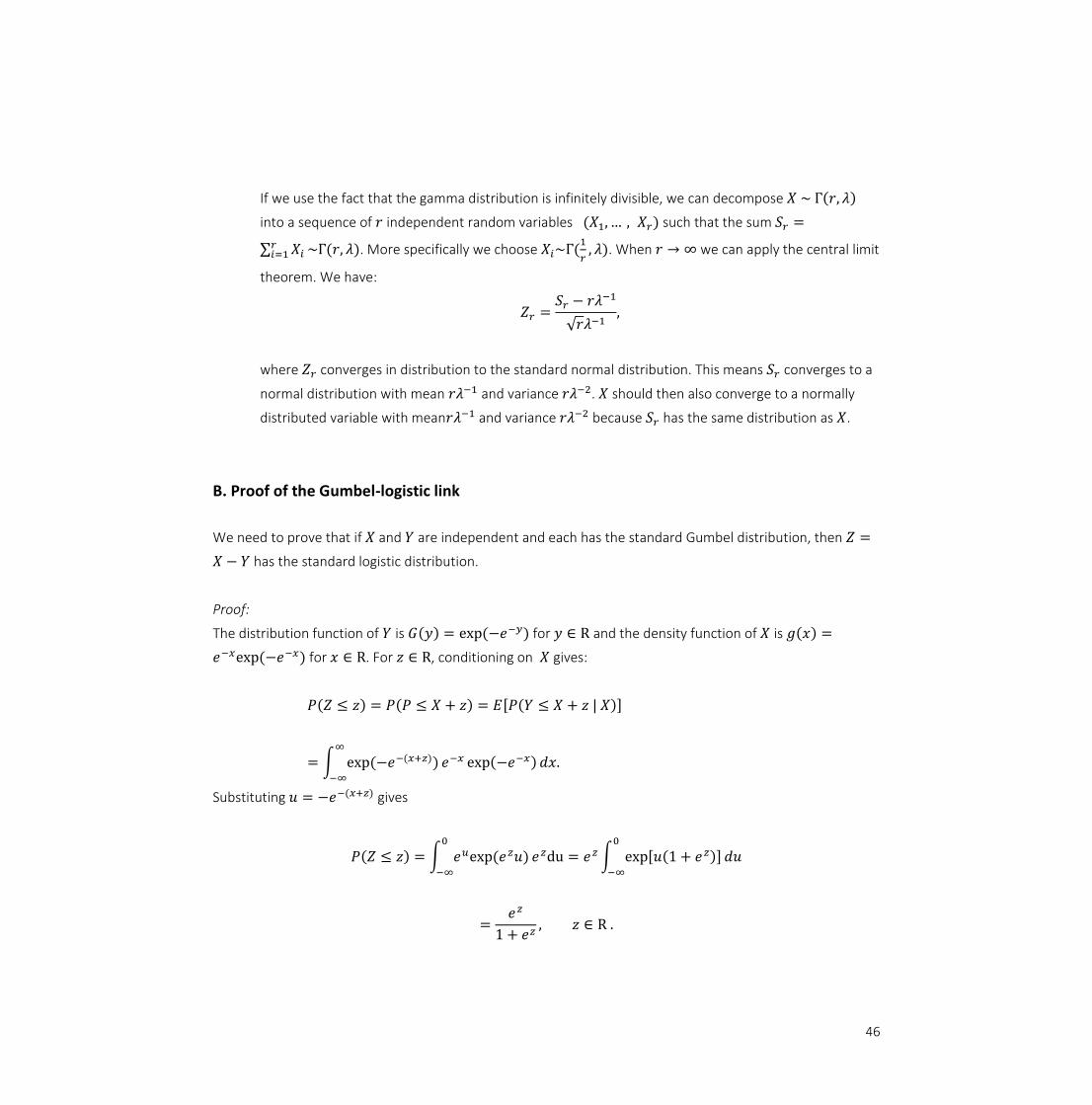
46
If we use the fact that the gamma distribution is infinitely divisible, we can decompose 𝑋 ~ Γ(𝑟, 𝜆)
into a sequence of 𝑟 independent random variables (𝑋1, … , 𝑋𝑟) such that the sum 𝑆𝑟 =
∑ 𝑋𝑖𝑟𝑖=1 ~Γ(𝑟, 𝜆). More specifically we choose 𝑋𝑖~Γ(
1
𝑟, 𝜆). When 𝑟 → ∞ we can apply the central limit
theorem. We have:
𝑍𝑟 =𝑆𝑟 − 𝑟𝜆−1
√𝑟𝜆−1,
where 𝑍𝑟 converges in distribution to the standard normal distribution. This means 𝑆𝑟 converges to a
normal distribution with mean 𝑟𝜆−1 and variance 𝑟𝜆−2. 𝑋 should then also converge to a normally
distributed variable with mean𝑟𝜆−1 and variance 𝑟𝜆−2 because 𝑆𝑟 has the same distribution as 𝑋.
B. Proof of the Gumbel-logistic link
We need to prove that if 𝑋 and 𝑌 are independent and each has the standard Gumbel distribution, then 𝑍 =
𝑋 − 𝑌 has the standard logistic distribution.
Proof:
The distribution function of 𝑌 is 𝐺(𝑦) = exp (−𝑒−𝑦) for 𝑦 ∈ R and the density function of 𝑋 is 𝑔(𝑥) =
𝑒−𝑥exp (−𝑒−𝑥) for 𝑥 ∈ R. For 𝑧 ∈ R, conditioning on 𝑋 gives:
𝑃(𝑍 ≤ 𝑧) = 𝑃(𝑃 ≤ 𝑋 + 𝑧) = 𝐸[𝑃(𝑌 ≤ 𝑋 + 𝑧 | 𝑋)]
= ∫ exp (−𝑒−(𝑥+𝑧))∞
−∞
𝑒−𝑥 exp(−𝑒−𝑥) 𝑑𝑥.
Substituting 𝑢 = −𝑒−(𝑥+𝑧) gives
𝑃(𝑍 ≤ 𝑧) = ∫ 𝑒𝑢exp (𝑒𝑧𝑢)0
−∞
𝑒𝑧du = 𝑒𝑧 ∫ exp[𝑢(1 + 𝑒𝑧)] 𝑑𝑢0
−∞
=𝑒𝑧
1 + 𝑒𝑧, 𝑧 ∈ R .
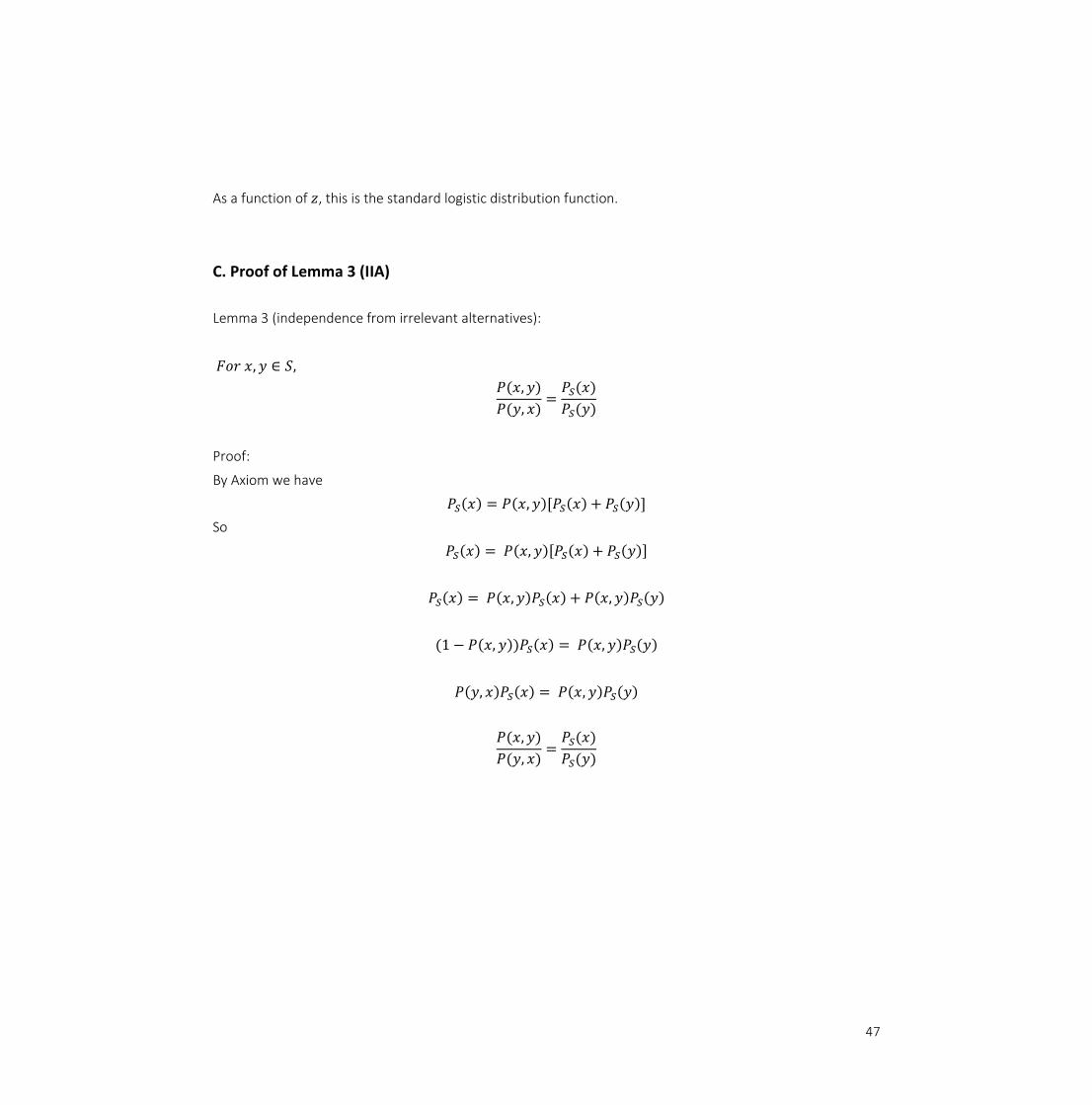
47
As a function of 𝑧, this is the standard logistic distribution function.
C. Proof of Lemma 3 (IIA)
Lemma 3 (independence from irrelevant alternatives):
𝐹𝑜𝑟 𝑥, 𝑦 ∈ 𝑆,
𝑃(𝑥, 𝑦)
𝑃(𝑦, 𝑥)=
𝑃𝑆(𝑥)
𝑃𝑆(𝑦)
Proof:
By Axiom we have
𝑃𝑆(𝑥) = 𝑃(𝑥, 𝑦)[𝑃𝑆(𝑥) + 𝑃𝑆(𝑦)]
So
𝑃𝑆(𝑥) = 𝑃(𝑥, 𝑦)[𝑃𝑆(𝑥) + 𝑃𝑆(𝑦)]
𝑃𝑆(𝑥) = 𝑃(𝑥, 𝑦)𝑃𝑆(𝑥) + 𝑃(𝑥, 𝑦)𝑃𝑆(𝑦)
(1 − 𝑃(𝑥, 𝑦))𝑃𝑆(𝑥) = 𝑃(𝑥, 𝑦)𝑃𝑆(𝑦)
𝑃(𝑦, 𝑥)𝑃𝑆(𝑥) = 𝑃(𝑥, 𝑦)𝑃𝑆(𝑦)
𝑃(𝑥, 𝑦)
𝑃(𝑦, 𝑥)=
𝑃𝑆(𝑥)
𝑃𝑆(𝑦)

48
References Agresti, A. (2002). Categorical Data Analysis, Second Edition. Wiley Series in Probability and Statistics. Akaike, H. (1973). Information theory and an extension of the maximum likelihood principle. Budapest: Akadémiai Kiadó. Bauml, K. H. (1994). Upright versus upside-down faces: How interface attractiveness varies with orientation. . Percept.
Psychophys. 56, 163–172. Block, D. H., & Marschak, J. (1960). Random Orderings and Stochastic Theories of Responses. Stanford, California:
Stanford University Press. Bradley, R., & Terry, M. (1952). Rank analysis of incomplete block designs I: The method of paired comparisons.
Biometrika, 39, 324–345. Cattelan. (2009). Correlation models for paired comparison data. Ph.D. thesis. Dept. Statistical Sciences, Univ. Padua. Cattelan. (2012). Models for Paired Comparison Data: A Review with Emphasis on Dependent Data. Statist. Sci. 27,
Number 3, 412-433. Cayley, A. (1859). Sixth Memoir on Conics. §209-229. Daniels, H. E. (1950). Rank Correlation and Population Models. Journal of the Royal Statistical Society, Ser. B, 12, 171-
181. Davidson, R. (1970). “On Extending the Bradley-Terry Model to Accommodate Ties in. Journal of the American Statistical
Association, 65, 317–328. Dawkins, R. (1969). Animal Behavior. Animal Behavior 17, 134-141. Diaconis, P. (1988). Group representations in probability and statistics. Institute of Mathematical Statistics. Engledrum, P. G. (2000). Psychometric Scaling: A Toolkit for. Winchester: Imoteck Press. Hamming, R. W. (1950). Error detecting and error correcting codes. Bell System Technical Journal, 29 (2), 147–160. Henery, R. J. (1992). An Extension to the Thurstone-Mosteller Model for Chess. Journal of the Royal Statistical Society.
Series D (The Statistician) Vol. 41, No. 5 , 559-567. Kendall. (1948). Rank Correlation Methods. Charles Griffin & Company Limited. Luce. (1959). Individual choice behavior: a theoretical analysis. New York: Wiley. Luce, R., & Suppes, P. (1965). Preference, Utility, and Subjective Probability. New York: Wiley. Mallows, C. (1957). Non-null ranking models. . Biometrika, 44(1), 114-130. Marden, J. I. (1996). Analyzing and Modeling Rank Data. CRC Press. Maydeu-Olivares, & Bockenholt. (2008). Modeling subjective health outcomes: Top 10 reasons to use Thurstone's
method. Medical Care, 46, 346-348. Mihram, G. (1975). A generalized extreme-value density. South African Statistical Journal 9, 153-162. Spearman, C. (1904). The proof and measurement of association between two things. American Journal of Psychology
15, 72–101. Stern. (1987). Gamma Processes, Paired Comparisons and Ranking "A Continuum of Paired Comparison Models".
Biometrika. Stern. (1990). Models for Distributions on Permutations. Journal of the American Statistical Association 85(410), 558-
564. Thurstone. (1927). A Law of Comparative Judgment. Psychological Review. 34 (4), 273–286. Thurstone. (1928). "Attitudes Can Be Measured.". American Journal of Sociology 33, 529-554. Torgerson, W. (1958). Theory and Methods of Scaling. New York: Wiley. Wickelmaier, & Choisel. (2007). Evaluation of multichannel reproduced sound: scaling auditory attributes. Journal of the
Acoustical Society of America 121, 388-400. Yelott, J. I. (1977). The Relationship between Luce's Choice Axiom, Thurstone's Theory of Comparative Judgment, and
the Double Exponential Distribution. Journal of Mathematical Psychology, 109-144.
Recommended