Staff Working Paper ERSD-2012-08 Date: April 2012
World Trade Organization
Economic Research and Statistics Division
Food Prices and the Multiplier Effect of Export Policy
Paolo E. Giordani Nadia Rocha
LUISS "Guido Carli" University World Trade Organization
Michele Ruta
World Trade Organization
Manuscript date: April 2012
Disclaimer: This is a working paper, and hence it represents research in progress. This
paper represents the opinions of the author(s), and is the product of professional research. It
is not meant to represent the position or opinions of the WTO or its Members, nor the official
position of any staff members. Any errors are the fault of the author(s). Copies of working
papers can be requested from the divisional secretariat by writing to: Economic Research and
Statistics Division, World Trade Organization, Rue de Lausanne 154, CH 1211 Geneva 21,
Switzerland. Please request papers by number and title.
Food Prices and the Multiplier Effect of
Export Policy∗
Paolo E. Giordani
LUISS "Guido Carli" University
Nadia Rocha
World Trade Organization
Michele Ruta
World Trade Organization
April 2012
Abstract
This paper studies the relationship between export policy and food prices. We show that,
when individuals are loss averse, food exporters may use trade policy to shield the domestic
economy from large price shocks. This creates a complementarity between the price of food in
international markets and export policy. Specifically, unilateral actions by exporting countries
give rise to a "multiplier effect": when a shock in the international food market drives up (down)
its price, governments respond by imposing export restrictions (subsidies), thus exacerbating the
initial shock and soliciting further export activism. We test this theory with a new dataset that
comprises monthly information on trade measures across 125 countries and 29 food products
for the period 2008-10, finding evidence of a multiplier effect. Global restrictions in a product
(i.e. the share of international trade covered by export restrictions) are positively correlated
with the probability of imposing a new export restriction on that product, especially for staple
foods. Large exporters are found to be more reactive to restrictive measures, suggesting that the
multiplier effect is mostly driven by this group. Finally, we estimate that a 1 per cent surge in
global restrictions increased international food prices by 1.1 per cent on average during 2008-10.
These findings contribute to inform the broader debate on the proper regulation of export policy
within the multilateral trading system.
Keywords : Loss aversion; Export policy; Multiplier effect; Food crisis; WTO.
JEL Classification : F13, F59, Q02, Q17.
∗Acknowledgments: We would like to thank Willy Alfaro, Simon Evenett, Gabriel Felbermayr, Caroline Freund,Robert Gulotty, Lee Ann Jackson, Nuno Limao, Marcelo Olarreaga, Gianluca Orefice, Roberta Piermartini, Frederic
Robert-Nicoud and seminar participants at the WTO, ETSG, LUISS, University of Munich, University of Frankfurt,
and the First IMF/WB/WTO Trade Workshop for comments and suggestions. We also thank Joelle Latina for excellent
research assistance. Remaining errors are our responsibility. Michele Ruta gratefully acknowledges hospitality at the
International Trade Department of CES-ifo during the early stages of this research project. Disclaimer: The opinionsexpressed in this paper should be attributed to the authors. They are not meant to represent the positions or opinions
of the WTO and its Members and are without prejudice to Members’rights and obligations under the WTO.
1
1 Introduction
International food prices have been a key policy concern in recent times. Figure 1 illustrates the extent
to which the 2006-2007 and the 2008-2010 periods differ from the preceding two decades, justifying
the labeling of "food crises". While a large number of factors may have contributed to the sudden
and rapid spikes in food prices (e.g. reduction in key food stocks, increasing demand in emerging
economies, financial speculation, changes in monetary policy in leading economies), several observers
have pointed out that trade policy may be part of the problem of escalating prices.1 Export policy,
in particular, has been on the spotlight. As Pascal Lamy, the Director General of the World Trade
Organization (WTO), put it: "export restrictions play a direct role in aggravating food crises" (Lamy,
2011a). Figure 2 corroborates this view by showing a positive correlation between export restrictions
and the global price of food in 2009 and 2010.2 This motivates our key research question: how does
export policy interact with food prices? Any proposal of reform of the current rules presiding the
multilateral trading system needs to depart from a better understanding of this relationship.
INSERT FIGURES 1 AND 2 HERE
Our view can be very simply stated. When trade policy aims at shielding the domestic market from
unfavorable developments in the world market, export measures have a "multiplier effect". Specifically,
high prices of food may trigger a series of export restrictions that exacerbate the rise of the world
price that, in turn, feeds into even more restrictive policies. Similarly, low prices of food may lead
exporting governments to set export promotion measures that lower the world price and induce further
support to exports. This paper presents a micro-founded model of this interaction between export
policy and food prices (both under the case of small and of large exporting economies) and tests its
main prediction with trade policy data for the period 2008-10.
The theory is based on recent developments in the literature on behavioral economics and trade
policy (Freund and Ozden, 2008, and Tovar, 2009). This literature modifies an otherwise standard
trade model to account for the empirical fact that individuals value losses more than gains (loss aver-
sion). In this setting, preventing losses looms large in the government’s objective function, something
that helps explain observed export policy in the food sector. When the world food market is hit by a
negative price shock, food producers experience a welfare loss. A welfare maximizing government can
(and will) offset this loss by offering an export subsidy. On the contrary, when the world food price
is high, consumers face loss aversion and the government responds by imposing an export restriction.
Finally, when global food prices are at intermediate levels, there is no rationale for government inter-
vention to prevent losses and policy makers face the standard incentives in setting trade policy (hence,
the unilaterally optimal policy is free trade for a small open economy and an export tax for a large
exporter).3
1A partial list includes Anderson and Martin (2011), Chaffour (2008), Bouet and Laborde (2010), Hochman et al.
(2010), Headey (2011).2Appendix Figure C1 provides a breakdown of the data for certain important food sectors.3A model of trade under loss aversion is not the only framework that would support that export policy is a function
of the international price of food. Gouel and Jean (2012) show that consumers’risk aversion may provide a rationale for
2
Small exporters take world prices as given and have, individually, no impact on global markets.
However, as they all face the same international price of food and have similar incentives to insulate
the domestic food market in presence of loss aversion, their simultaneous behavior will have aggregate
consequences. Intuitively, the international price of food is determined by the equilibrium of global
export supply and import demand. A simultaneous imposition of export subsidies in response to low
food prices or export taxes to high prices has systemic implications as it shifts the global export supply
outward or inward respectively. We show that these policy actions can give rise to a multiplier effect.
Focus on export restrictions (but the same logic applies to export subsidies). When a shock to the
world food market pushes up the global price of food, exporters set export restrictions to offset the
world price shock and avoid consumer loss aversion. Because all exporting countries impose restric-
tions, however, the world price of food increases, which makes the initial policy response inadequate
to compensate consumers. The higher food price induces further restrictions as governments strive
to maintain a stable domestic price. Note that, differently from the initial response, further increases
in restrictions are not driven by fundamentals, but are only a reaction to the restrictions imposed by
the other exporters. This is precisely the idea behind the multiplier effect.
The logic just discussed extends to the case where exporting countries’policy decisions have an
impact on global markets. Contrary to small economies, large exporters do not take the international
price of food as given and choose their trade policy strategically. In this context, when loss aversion
looms large in the governments’objective function (i.e. when the world price of food is hit by a positive
or negative shock), export policies are strategic complements. This complementarity in export policy
can rationalize the observed pattern of trade measures in food markets characterized by few large
exporters.4 Intuitively, if a large exporter raises its tax on exports, it increases the world price of food,
which in turn leads other exporting governments to further restrict their exports to avoid consumers’
losses. Similarly, by depressing the price of food in international markets, higher export subsidies by
a large exporter induce others to take the same course of action in order to offset the welfare loss
of domestic food producers. This strategic complementarity of large exporters’trade policy creates
a multiplier effect that magnifies the consequences of exogenous shocks to the international price of
food.
We test empirically the predictions of the model for the years 2008-10. During this period, food
prices have been almost 60 per cent higher than average prices between 1990 and 2006 and export
policy has been dominated by restrictive measures. We investigate two issues. First, we study the
determinants of export restrictions. Specifically, we employ a probability model to examine whether
exporters set trade policy in response to measures implemented by other governments in order to
protect their domestic market. Second, we estimate a simultaneous equation model to assess the
trade policy activism in presence of high world food prices. In alternative, Appendix A1 proposes a framework where
governments are averse to inequality across different groups in society. However, as argued in Anderson and Martin
(2011), the trade policy behavior arising from a model based on loss aversion is consistent with the observed conduct
of several governments (see also Ivanic et al., 2011).4 In the words of the WTO Director General: "In response to the crises, some started looking further inwards, and
we saw a whole host of export restrictions flourish. These export restrictions had a domino, market-closing, eff ect,
with one restriction bringing about another" (Lamy, 2011b). Note that we prefer to refer to this effect as a multiplier,
rather than a domino, effect, as the latter generally denotes a linear sequence of events with no feedback (i.e. backward
reaction), which is instead an implication of our model.
3
overall impact of export restrictions on food prices.
We use a new data set on trade policy measures from the WTO Monitoring exercise and comple-
ment it with additional information from the Global Trade Alert. This novel dataset contains monthly
information on export restrictions in the food sector across 125 countries at the 4-digit level for the
2008-2010 period. The level of global restrictions on a product, measured by the share of international
trade covered by export restrictions, vary substantially in our sample, ranging from 0.001 per cent for
swine meat to 50 per cent for cocoa beans. In the whole food sector, 9 per cent of trade is covered by
export restrictions. When we focus on important food products such as staple foods, global export
restrictions are higher, covering 22 per cent of trade on average in the period of observation.
The empirical results strongly support the existence of a multiplier effect in food export policy. The
level of global restrictions on a food product has a positive and significant impact on the probability
that a government imposes a new restriction to the exports of that product. We show that this
finding is mostly driven by large exporters and that it is robust to several specifications and to
potential endogeneity problems. Finally, results from the simultaneous equations estimation show
that global restrictions have considerably increased world food prices in 2008-10. On average, a 1 per
cent surge in the share of trade covered by export restrictions is associated to a 1.1 per cent increase
in international food prices. These findings support the view that export policy was an important
contributing factor to the global food crisis in 2008-10.
There is a wide body of related literature that deals with export policy in the agricultural sector,
and we do not attempt to summarize it here. Studies generally focus either on export restrictions or
on export subsidization. In the first group, the closest to our paper are the afore-mentioned Anderson
and Martin (2011) and Bouet and Laborde (2011). They share the view that trade policy in the food
sector can aim at insulating the domestic market and that these policy actions may contribute to
disrupt international food markets. The focus of these analyses is at the same time broader and more
limited than ours. First, their argument is that raising food prices can be the result of a collective
action problem between exporters on one side and importers of food on the other, while our model
only focuses on exporting countries. Second, we provide a fully micro-founded model and analytically
prove the existence of a multiplier effect in export policy. Finally, our empirical analysis uses actual
information on export policy measures rather than indirect estimates based on agricultural distortions
in selected food sectors (Anderson and Martin, 2011) or simulations (Bouet and Laborde, 2011).
Bagwell and Staiger (2001) provide a political economy model of export subsidies in agricultural
products that shares some similarities with ours. In particular, they show that, when governments
weigh suffi ciently the interests of producers, exporting countries may end up in an ineffi cient equi-
librium (a subsidy war) where export subsidies are high and world food prices low. While the two
approaches are not mutually exclusive, two intriguing features of our framework appear to be con-
sistent with observed export policy in the food sector. First, exporters respond to the level of the
international price, so that whether the government chooses an export subsidy, tax or free trade
depends on the conditions in the international food market. Second, the fact that prices of several
commodities are characterized by long periods of stability interrupted by sudden and sharp disruptions
that (we show) can be amplified by export policy choices.
The paper is structured as follows. Section 2 presents the basic structure of the model of trade
policy under loss aversion. The unilateral food export policy for a small exporting country is deter-
4
mined in Section 3, while the result of a multiplier effect in export policy is derived in Section 4. The
case of large exporters is analyzed in Section 5. We discuss the assumptions of the model in Section
6. Section 7 studies the empirical relevance of the main predictions of the theory. Policy implications
for the design of multilateral trade rules are analyzed in the Conclusions. All the proofs are relegated
to a technical appendix.
2 The model: Food prices and loss aversion
Consider a small open economy producing two goods, a numeraire and a commodity that we refer to as
food. The economy imports the numeraire good at a unitary world price and exports food at the world
price, p∗. The numeraire is produced with labor alone, using a constant returns to scale technology
(y0 = l0). Assuming that labor supply is suffi ciently large, the wage rate in the economy is fixed and
equal to one. Food is produced using labor and a specific factor in fixed supply, land (L). Technology
in the food sector also exhibits constant returns to scale and takes the form y = f(l, L). Given the
domestic price of food, p, the return to the owners of the specific factor is π (p) = maxl
[pf(l, L)− l].Finally, the domestic output of food is y (p) = π′ (p).
The economy is composed of a continuum of individuals of measure one with identical preferences.
We assume that agents derive utility from consumption of the two goods and from deviations from
their reference-dependent utility. Specifically, the utility function has the following separable form:
U = c0 + u(c)− I · h(U − c0 − u(c)), (1)
where c0 is the consumption of the numeraire good and c is food consumption. Function u(·) has thestandard properties (u′(·) > 0, u′′(·) < 0). Function h(·) captures the behavioral features of the model.In particular, h(·) is increasing in the difference between a reference level U and the actual utility
from consumption (i.e. h′(·) > 0), and it displays diminishing sensitivity to losses (i.e. h′′(·) < 0). I
is an indicator variable that takes value one whenever the utility falls strictly below the reference level
and zero otherwise. This utility structure supports the idea that individuals experience a welfare loss
when they achieve a level of utility inferior to what they are accustomed to, but do not perceive any
additional welfare gain when utility is higher than usual.5 Since one of the two goods in this economy
is food, it is tempting to associate the reference utility U to a subsistence level of consumption, which
may be considered unacceptably low and might justify policy intervention.
Maximizing utility given by (1) subject to the budget constraint gives the individual demand
function of food d(p) = [u′(c)]−1, while remaining income is spent on the numeraire good, c0 =
E − pd(p), where E is individual income level. The government can use trade policy to intervene in
the food sector.6 Specifically, the policy maker can impose an export tax or an export subsidy that
5Freund and Ozden (2008) and Tovar (2009) have introduced loss aversion in a model of trade policy and find that
this behavioral extension explains several features of the observed pattern of trade protectionism. Classic works on
reference-dependent utility include Kahneman and Tversky (1979), Tversky and Kahneman (1991), and Koszegi and
Rabin (2006). Tversky and Kahneman (1981), Samuelson and Zeckhauser (1988), and Camerer (1995), among others,
provide experimental evidence supporting this preference structure.6As confirmed by the evidence provided in this paper and in the studies discussed in the Introduction, governments do
indeed actively use trade policy in food sectors. An important question, not addressed in this paper, is why governments
use more distortive policies, such as trade policy, rather than more effi cient tools, such as domestic measures. One reason
5
create a wedge between the international and the domestic price of food. Formally, p = p∗ + s, where
positive values of s correspond to an export subsidy and negative values to an export tax, defined as
t = −s. Government revenue is, therefore, given by
GR(p) = t [y(p)− d(p)] ≷ 0. (2)
We assume that, whenever positive, the government redistributes revenue uniformly to all agents,
while lump-sum taxes are used to finance a negative budget.7
We denote by α the fraction of the population that owns land (land owners/producers). Agents in
the remaining share of the population (1−α) have one unit of labor each that they supply inelasticallyto the market. We refer to this latter group as workers/consumers. In this setting, interests in society
are radically different, as a change in the price of food affects different social groups in opposite ways.
Intuitively, owners of land see their income and welfare positively tied to the domestic price of food,
while workers are hurt by a surge in food prices as this limits their consumption possibilities. A fall in
the domestic price of food has the opposite effect on the utility of these two social groups. Formally,
the indirect utility of a worker and of a land owner can be written respectively as
V lp (p) = 1 + CS(p) +GR(p)− I l · h[V l(p)− 1− CS(p)−GR(p)
](3)
and
V Lp (p) =π(p)
α+ CS(p) +GR(p)− IL · h
[V L(p)− π(p)
α− CS(p)−GR(p)
], (4)
where CS(p) = u [d(p)]− pd(p) is consumer surplus. The indicator variable I l is equal to 1 whenever
V l(p) > 1 + GR(p) + CS(p) and zero otherwise. The indicator variable IL is equal to 1 whenever
V L(p) > π(p)/α+GR(p) + CS(p) and zero otherwise.
As labor income is constant, the extent of loss aversion for workers is determined by consumer
surplus and government revenue. Since the sum of these terms is strictly decreasing in p, their
reservation utility corresponds to a unique reference price denoted by p. More precisely, according
to condition (3), whenever domestic food prices are high (p > p), expected utility falls below the
reference point, and workers/consumers incur an additional welfare loss captured by the term h(·).When instead food prices are low (p < p), they do not derive any additional utility.
On the other hand, assuming that land owners are a suffi ciently small fraction α of the total
population, they enjoy only a tiny share of the surplus generated by food consumption and perceive
a negligible fraction of the tax revenue (or cost). For individuals in this group, an increase in the
domestic price of food strictly increases utility, as the positive effect on the rent from the specific factor
dominates the loss in consumer surplus and government revenue. As a result, the reference utility
for producers corresponds to the unique price p. According to condition (4), whenever the domestic
price of food falls below this threshold level (p < p), they perceive a decline in their welfare, but no
may have to do with the availability of appropriate domestic policies, particularly in developing countries. Limao and
Tovar (2009) provide an alternative explanation based on a political economy argument.7The analysis of this paper focuses on export taxes that in our sample represent 20 per cent of total export restrictions.
As is well understood, this measure is equivalent to an export quota under the assumption that the quota rent is rebated
lump-sum. In addition to taxes and quotas, other export restrictions used in the 2008-10 period include prohibitions,
minimum export prices, technical barriers. See Table 3 for details.
6
additional welfare gain is incurred when land owners face a price of food higher than their reservation
price.8
3 Unilateral food export policy under loss aversion
This section explores the optimal export policy for a small open economy under loss aversion (Section
5 presents an extension to this basic framework where the economy is large in the international food
market). Total welfare is defined as
G(p) = W (p) +H(p), (5)
where standard social welfare (i.e., net of loss aversion) is the sum of labor income, revenue from the
specific factor, consumer surplus and government revenue
W (p) = (1− α) + π(p) + CS(p) +GR(p),
while loss aversion for the entire economy is
H(p) = − (1− α) I l · h[V l(p)− 1− CS(p)−GR(p)
]− αIL · h
[V L(p)− π(p)
α− CS(p)−GR(p)
].
The government sets trade policy to maximize social welfare given by condition (5). In this
framework where loss aversion affects welfare, there are several different scenarios that need to be
considered which depend on the level of the international price of food. In particular, there are three
main regions. A first area corresponds to the situation where the international price of food has
"intermediate" values, that is, when p∗ ∈[p, p]. In this case, the loss aversion term is null and the
optimal trade policy is the one that corresponds to free trade.9 When the international price is "low"
(i.e. p∗ < p) and when it is "high" (i.e. p∗ > p), the derivation of the optimal policy for a small
open economy is more complicated, as either land owners/producers or workers/consumers suffer an
additional welfare loss (i.e. H(·) 6= 0).
Consider first the case where the international price of food is below the lower-bound of the
reservation price, p (this is the case considered in previous literature). It can be shown that there
exists a region of compensating protectionism, where the government sets an export subsidy to fully
compensate producers for the welfare loss caused by the fall in the international price of food. In fact,
the first-oder condition (FOC) of social welfare (5) with respect to the domestic price, which takes
8To be clear, this model introduces a slightly different feature relative to Freund and Ozden (2008) and Tovar (2009).
These authors abstract from the effect that changes in prices have on consumer surplus and government revenue and
focus instead on the direct effect that these price changes have on the income of factor owners. This is a reasonable
assumption in their models where there are many consumption goods, none of which is supposed to represent a large
share of total consumption. The structure presented here is instead better suited to capture the fact that the poor,
particularly in developing countries, spend an important portion of their income on food. For example, the poorest
decile of the population in Nigeria, Vietnam and Indonesia spend respectively 70, 75, and 50 per cent of their income
on food (Ivanic et al., 2011).9The proofs of this and the following statements, which form the basis of Proposition 1 below, are provided in
footnote as they follow closely the work by Freund and Ozden (2008). When H(·) = 0, total welfare reduces to the
standard form: G(p) = W (p) = (1− α) + π(p) +CS(p) +GR(p). The optimal domestic price is determined by the first
order condition ∂W/∂p = (p∗ − p) [y′ − d′] = 0, which is satisfied for p = p∗.
7
into account that in this scenario land owners experience a loss (IL = 1), may or may not be satisfied
in the region(p∗, p
). Specifically, there is a critical level of the international price (call it pc < p) such
that, for p∗ ∈(pc, p
), the FOC is not satisfied in the relevant region, and we have a corner solution.10
In this case, the government sets trade policy so that the domestic price equals p, and the optimal
export subsidy is
s = p− p∗. (6)
If p∗ ≤ pc, the maximum is an interior solution. The government still imposes an export subsidy, but
in this case it does not fully compensate producers.11
Consider next the scenario in which the international price of food is high, that is, where the
price is above the reservation price of workers/consumers, p. Similarly to the previous scenario, it
can be shown that there exists a second region of compensating protectionism, where the policy maker
imposes an export tax to fully offset the welfare loss of consumers due to the increase in the world
price of food. The FOC of social welfare with respect to the domestic price of food, which takes into
account the additional welfare loss for workers (I l = 1), may or may not be satisfied in the region
(p, p∗), depending on whether the international price of food is below or above a threshold level,
denoted by pc > p. In particular, when p∗ ∈ (p, pc), the FOC is not satisfied in the relevant region,
and the government sets trade policy to maintain the domestic price of food at the reservation price
for workers p (corner solution).12 The corresponding optimal export tax is
t = p∗ − p. (7)
If instead p∗ ≥ pc, the optimal domestic price is an interior solution. The optimal trade policy is stillgiven by an export tax, which in this case does not fully compensate consumers.13
10The FOC can be expressed as
∂G
∂p= W ′ +H′ = (p∗ − p)x′ +
[(1− α) y + α(p∗ − p)x′
]· h′ = 0,
where x(p) = y(p) − d(p) is net export supply of food. Consider the case in which the international price falls from
p∗ = p to p∗ = p − ε. For ε small enough, W ′(p − ε) = 0, while H′(p − ε) > 0, which implies G′(p − ε) > 0. In this
case, the optimal domestic price of food is a corner solution and is equal to the reservation price for land owners, p. As
ε increases (and, hence, p∗ moves away from p), the loss aversion effect weakens due to diminishing sensitivity to losses
(h′′ < 0), while W ′(p) becomes more negative. This implies that there is a critical level of the world price p∗ =pc < p,
below which the optimal domestic price is an interior solution to the welfare maximizing problem.11 In particular, solving the FOC when H (·) 6= 0 gives the following export subsidy:
s
p∗ + s=
(1− α)h′
1 + αh′z
e,
where z ≡ y/x is the ratio of domestic output to exports and e ≡ (x′p) /x is the elasticity of export supply.12 In this case, the FOC is given by
∂G
∂p= W ′ +H′ = (p∗ − p)x′ + (1− α)
[−y + (p∗ − p)x′
]· h′ = 0.
The proof of this statement follows the same steps as in footnote 10. Specifically, for an international price of food
p∗ = p + ε, with ε small enough, W ′(p + ε) = 0, while H′(p + ε) > 0, which implies G′(p + ε) > 0. In this case, the
optimal domestic price of food is a corner solution, which equals the reservation price for workers p. As ε increases, the
loss aversion effect weakens, while W ′(p) becomes more negative. There is a critical level of the world price p∗ = pc > p,
above which the optimal domestic price becomes an interior solution.13 In particular, the export tax can be shown to be
t
p∗ − t= − (1− α)h′
1 + (1− α)h′z
e.
8
The optimal export policy for a small open economy under loss aversion is characterized in the
following
Proposition 1 For an international price of food p∗ ∈[p, p], the optimal export policy for a small
open economy is free trade. For p∗ < p, the optimal policy is an export subsidy; a region of full
producer compensation (i.e. where s = p− p∗) exists for p∗ ∈(pc, p
). For p∗ > p, the optimal policy
is an export tax; a region of full consumer compensation (i.e. where t = p∗− p) exists for p∗ ∈ (p, pc).
Proposition 1 establishes that the optimal food export policy for a small open economy under loss
aversion depends on the international price of food.14 This trade policy is depicted in Figure 3. The
government does not intervene in the food sector when international prices are at intermediate levels.
On the contrary, absent other tools to address loss aversion, a welfare maximizing government may use
export policy in food markets when the international price of food is low (i.e. below the reservation
price of land owners/producers, p) or high (above the reservation price of workers/consumers, p). In
the first case, the government imposes an export subsidy to offset the welfare loss for land owners. In
the second case, the policy maker sets an export tax aiming at decreasing the negative effect of high
food prices on the utility of workers. In both cases, the rationale behind export policy is the one of
offsetting (completely or in part) the effect that "extreme" conditions in international food markets
have on the welfare of domestic constituencies.
INSERT FIGURE 3 HERE
The model also has insights on the structure of export promotion or restriction. When the interna-
tional price of food moves slightly below the reservation price of producers (p) or above the reservation
price of consumers (p), the government intervenes to fully compensate the constituency that is incur-
ring a welfare loss. In other words, there is a range of world prices such that the policy maker sets
export policy to bring the domestic price at the reference level of the group that is experiencing loss
aversion. These areas are represented in Figure 3 by the region (p, pc) for export taxes and(pc, p
)for
export subsidies. Export intervention increases as the price of food diverges, since the policy aims at
fully compensating the losing constituency (i.e. taxes are augmented as food prices rise, subsidies are
increased as prices plunge). As the world price of food continues to diverge from the reference prices
of producers or consumers, the structure of export policy changes. Intuitively, the marginal cost of
trade intervention on welfare net of loss aversion increases, and diminishing sensitivity to losses makes
full compensation less attractive.15 Export subsidies (and taxes) are still used to offset increasingly
14Anecdotal evidence confirms that export policy in food sectors is often designed to stabilize domestic prices and avoid
losses for specific groups (see Piermartini, 2004). For instance, Papua New Guinea had in place an export tax/subsidy
rate for cocoa, coffee, copra, and palm oil equal to one-half the difference between a reference price (calculated as the
average of the world price in the previous ten years) and the actual price of the year.15More specifically, the expressions for subsidy and tax in footnotes 11 and 13 equate the marginal gain as a result of
reducing the constituency’s losses (land owners and workers respectively) to the marginal loss in standard social welfare
induced by the export measure. As is usual, the optimal trade intervention is affected by the ratio of output to exports
and the elasticity of export supply that influence the welfare cost of trade policy.
9
high (low) world food prices, but the optimal policy no longer aims at full compensation of the losing
constituency.
4 Food export policy and the multiplier effect
The previous section established that, under loss aversion, the government of a small economy may
have an incentive to use export taxes in response to high food prices in international markets and
export subsidies to offset low prices. As discussed, the aim is essentially to insulate the domestic
economy from large international price changes. Naturally, a trade measure by a small economy in
itself has no effect on world markets. However, if all exporting economies face similar incentives
to alter their trade policy in the same direction, an effect on the international price of food will
materialize which may induce a further policy response. This section provides a formalization of how
small exporters’collective action interacts with the international price of food.
Suppose that there exists a continuum of identical small countries, with the same features as in
the previous section and indexed along the interval [0, 1]. Since we are looking for symmetric market
equilibria, pose ti = t ∀i ∈ [0, 1]. The equilibrium condition in the international food market can be
written as
x (p∗ − t) = m (p∗) (8)
where m (p∗) is the global import demand of food,16 and x (p∗ − t) is the world export supply definedas
x (p∗ − t) =
1∫0
xi (p∗ − t) di.
Expression (8) implicitly defines the world price as a function of the export policies of all exporting
countries, p∗ (t). When t = 0, the international price corresponds to its free trade level (define
p∗ (0) ≡ p∗ft). It is also immediate to prove that p∗ is an increasing function of t, and in particular
that dp∗/dt ∈ (0, 1).17 Uniform trade policy responses by all exporters will alter the world price of
food. In particular, a simultaneous imposition of export taxes will result in higher international prices,
while export subsidies will depress the world price of food.
The above consideration and the findings of Proposition 1 highlight an important interaction
between export policy and food prices. Governments respond to high (low) food prices by imposing
export taxes (subsidies) that, if applied symmetrically, increase (decrease) the world price of food.
This may induce further increases in export taxes (subsidies). We refer to this as the multiplier effect
of export policy. Whether this multiplier effect will materialize or not depends on the conditions in
global food markets. When the world price of food is at intermediate levels (p∗ ∈[p, p]), governments
have no incentive to employ an active export policy and the multiplier effect is dormant. When,
16This section abstracts from changes in import policy. Subsection 6.2 discusses how results change when this
assumption is relaxed.17Define F (p∗, t) ≡ x (p∗ − t)−m (p∗). By the implicit function theorem,
dp∗
dt= −
dFdtdFdp∗
=
dxdp
dxdp− dm
dp∗,
which belongs to the interval (0, 1), as dx/dp > 0 and dm/dp∗ < 0.
10
instead, a world price surge (fall) raises governments’protection of consumers (producers) -as in the
regions of compensating protection-, a multiplier effect will characterize export policy.
For illustrative purposes, we focus on the price escalation effect of export taxes (export subsidies,
which depress the world price of food, can be discussed in a similar way). Assume that an exogenous
shock to the international market of food brings the international price under free trade to p∗ft > p.
This situation induces each policy maker in exporting countries to impose an export tax to shield
consumers by maintaining the level of the domestic food price at p. But as all exporters face the same
incentive and act similarly, the international price of food is pushed up by the fall in world supply.
The consequence of this price surge is another round of export taxes that, in turn, lead to higher
international prices and even higher export taxes. Note, however, that differently from the initial
export tax, which is the response to a shock in the world food market, subsequent increases in export
restrictions are the reaction to taxes set by all other exporters.
The key insights can be inferred by looking at Figure 4. The figure depicts (i) the optimal export
policy for a small open economy as a function of the international price of food (t(p∗)) and (ii) the
international price of food as a function of the (symmetric) tax imposed by exporters (p∗(t)) -the
latter is depicted as a linear function for illustrative purposes only (see example 1). The solution to
the system made up of these two functions, (p∗e, te), characterizes the equilibrium in the world market
of food and is represented as point E in Figure 4.18
INSERT FIGURE 4 HERE
The equilibrium can be described as the result of a process of consecutive tax increases across
exporting countries. For the international price p∗ft > p, the corresponding export tax for each
individual country is optimally set at level t1. However, if all exporters set a tax t1, there is an excess
demand in the global food market and the international price of food increases to p∗1. At this price,
the initial level of the export tax is ineffi ciently low, and each policy maker increases restrictions
to t2. This multiplicative process stops where the international price curve (p∗(t)) intersects the
optimal export policy (t(p∗)): at that point, the uncoordinated behavior of exporters has caused the
equilibrium international price of food to increase relative to its initial level under free trade.19
We formally characterize the relationship between export policy and food prices in Proposition 2,
in which we show that the equilibrium reaction to an exogenous shock to supply or demand of food is
greater than the partial response by each exporting country taking the policy of the others as given.
Any shock to supply or demand can be captured by changes in p∗ft, which univocally determines the
position of function p∗(t) in Figure 4.
18The proof of the uniqueness of this equilibrium is a straightforward geometric implication of the two following
general properties of the model: (i) dp∗/dt ∈ (0, 1), (ii) dt/dp∗ = 1 along the regions of compensating protectionism.19While the focus of the above discussion is on export taxes, the logic of the result also applies to export subsidies
to food products. Low prices induce governments to offer subsidies to compensate producers. However, as all exporters
face similar incentives and enact the export promotion policy at the same time, the effect is to increase the export supply
of food in world markets and further depress prices. The multiplier effect in export policy determines an equilibrium of
high subsidies and low food prices relative to free trade.
11
Proposition 2 Along the regions of compensating protectionism identified in Proposition 1, a multi-
plier effect characterizes export policy. In particular, it is
dt
dp∗ft= θ
∂t
∂p∗ft,
where θ > 1. There is no multiplier effect when the international price belongs to the interval[p, p].
Intuitively, following a shock to the price of food, a multiplier effect in export policy is present
when the aggregate policy response to the shock exceeds the individual one. Specifically, the initial
export tax (subsidy) imposed by an individual exporter in response to a high (low) price of food is
smaller than the equilibrium measure set by that policy maker and by all other exporting governments.
Example 1. Let us provide a simple example of this multiplier effect for an economy with linearimport demand and export supply. In particular, suppose xi (p∗ − t) = α + β (p∗ − t) ∀i ∈ [0, 1] and
m (p∗) = γ − δp∗, with α, β, γ, δ ∈ R+ and where t is a specific export tax (or subsidy if lower than
zero). Equilibrium in the world market of food implies
1∫0
[α+ β (p∗ − t)] di = γ − δp∗,
from which we obtain the world price as
p∗ = p∗ft + ηt,
where η ≡ β/ (β + δ) and p∗ft ≡ (γ − α) / (β + δ) (the untaxed world price). Let us now analyze what
happens when p∗ft > p (the case in which p∗ft < p is analogous and thus omitted). Along the region
of compensating protection, each country i poses ti = p∗ − p. In a symmetric market equilibrium it
holds p∗ = p∗ft + ηt
t = p∗ − p,
from which it results
t∗ =1
1− η(p∗ft − p
)> 0.
Then it isdt
dp∗ft= θ
∂t
∂p∗ft,
where
θ ≡ 1
1− ηis the limit of a geometric series of ratio η, which in standard economic terminology is usually referred
to as the multiplier. This multiplier is finite and strictly higher than 1 as η ≡ β/ (β + δ) ∈ (0, 1).
12
5 Food export policy with large exporters
Consider an economy composed of n large identical exporters, each characterized by the same tech-
nology and preferences as the small economies described in Section 2. The only crucial difference is
that large exporters do not take the world price of food as given: in deciding their trade policy, these
countries take into account the effect of their measures on the world price.
As seen before, the equilibrium value of the world price of food is the one which equalizes import
demand and export supply of food. Denote by m (p∗) the global import demand and by xi (p∗ − ti)the export supply of food in country i. Since the n countries share the same fundamentals, it is
xi (·) = x (·) ∀i = 1, .., n. Equilibrium in the world market implies
n∑i=1
x (p∗ − ti) = m (p∗) (9)
The expression above implicitly defines the world price as a function of trade policy of all exporting
countries, p∗ (t), where t ≡ t1, .., ti, .., tn. If t = 0, then p∗ (0) = p∗ft.
Now consider a generic country i. Its optimal unilateral policy is the one which maximizes
Gi (ti, p∗ (t)) = Wi (ti, p
∗ (t)) +Hi (ti, p∗ (t)) , (10)
where, as before, standard social welfare (i.e. net of loss aversion) is the sum of labor income, revenue
from the specific factor, consumer surplus and government revenue:
Wi (ti, p∗ (t)) = (1− α) + π (ti, p
∗ (t)) + CS (ti, p∗ (t)) +GR (ti, p
∗ (t)) , (11)
while the loss aversion term is defined as
Hi (ti, p∗ (t)) = − (1− α) I l · h
[V l(p)− 1− CS (ti, p
∗ (t))−GR (ti, p∗ (t))
]−αIL · h
[V L(p)− π (ti, p
∗ (t))
α− CS (ti, p
∗ (t))−GR (ti, p∗ (t))
].
Parameters p and p are to be interpreted as follows. When the domestic price lies inside interval[p, p], the loss aversion term is null, and each government maximizes function (11). When instead
p > p (p < p), then I l = 1 (IL = 1), and each government maximizes function (10).
The optimal policy chosen by country i directly depends on the policies chosen by all other export-
ing countries. The strategic interaction of these countries can be described as a simultaneous game
with n players, each deciding the trade policy which maximizes its own welfare. Given the symmetric
structure of this game, we look for symmetric Nash equilibria. In analogy to the previous case of small
exporting countries, different scenarios must be considered depending on whether or not loss aversion
plays a role in the problem of welfare maximization.
If loss aversion does not play any role, the best response function of each country i comes from
the maximization of (11), and a candidate symmetric Nash equilibrium is given by the solution to
the system made up of the n best response functions (one for each country): call it t ≡t, .., t
.20
Denote by p ≡ p∗(t)− t the domestic price resulting from all large exporters implementing policy t.
If p ∈[p, p], then the candidate solution t ≡
t, .., t
is indeed a Nash equilibrium of the game.
20As is well-known from the theory and supported by recent evidence (in particular, Broda et al. 2008), countries
that have power in international markets have an incentive to set trade policy in order to obtain a terms-of-trade gain
13
If instead p < p or p > p, then Hi (·) > 0 ∀i, loss aversion does play a role, and the n bestresponse functions are determined via the maximization of (10) for any country i. In this case, the
equilibrium policy of the whole exporting region may be one of compensating protectionism, where
the policy maker of each country chooses its export tax (subsidy) to maintain the domestic price at
the reservation level of consumers (producers).
To gain an intuition of this statement, suppose that p > p, and denote by t ≡t, .., t
the solution
to the system made up of the n best response functions obtained from the maximization of (10) with
IL = 0 and I l = 1.21 If the corresponding domestic price (p ≡ p∗(t)− t) is higher than p, then tax t
is an equilibrium resulting from an interior solution. If instead p is lower than p, the equilibrium tax
results from a corner solution in which t is the tax that keeps the domestic price constant at level p.
An analogous reasoning holds when p < p. In the next proposition we formally prove this statement
and, in particular, we show that, in analogy to the small country case, two intervals of values for the
-exogenously given- free trade world price of food (p∗ft) exist, for which the equilibrium policy of the
exporting region is one of compensating protectionism.
Proposition 3 (i) For any p∗ft ∈(pft, p
cft
), the equilibrium policy for large exporters is a tax t ≡ (t, ..., t)
such that p∗(t, p∗ft
)− t = p (i.e. full consumer compensation). (ii) For any p∗ft ∈
(pcft, pft
),
the equilibrium policy for large exporters is a subsidy s ≡ (s, ..., s) (or a tax if s < 0) such that
p∗(s, p∗ft
)+ s = p (i.e. full producer compensation).
As in the small country case, along the two regions of compensating protectionism, the loss aversion
effect is so strong that all governments set export policy to maintain their domestic price at the
reservation level of land owners/producers or workers/consumers. In what follows we show that,
when this is the case, export policy is still characterized by a multiplier effect. We can now enunciate
the following
Proposition 4 Along the regions of compensating protectionism identified in Proposition 3: (i) coun-tries’export policies are strategic complements, that is dti/dt−i ∈ (0, 1) for i = 1, ..., n; (ii) a multiplier
effect characterizes export policy, that is
dtidp∗ft
= Φ∂ti∂p∗ft
∀i = 1, .., n,
where Φ > 1.
(the optimal tariff argument). It can be easily shown that the equilibrium policy in the absence of loss aversion is an
export tax. Specifically, welfare maximizing governments set
t =1
[nζ + (n− 1)e],
where 1/n is the share of each country’s exports on total exports, and ζ is the foreign import demand elasticity. The
equilibrium tax goes to zero as n→∞ (as in Section 3), and it reaches the standard optimal export tax level for n = 1.
Whenever n > 2, welfare of exporting countries would increase if they could coordinate on a higher export tax (see,
Limao and Saggi, 2011, for a formal discussion of this point in the case of multiple symmetric importers).21The fact that t > t is formally proven in the proof of Proposition 3. It is, however, rather intuitive that the optimal
tax policy when consumers’loss aversion matters is strictly higher than the optimal tax when it does not matter.
14
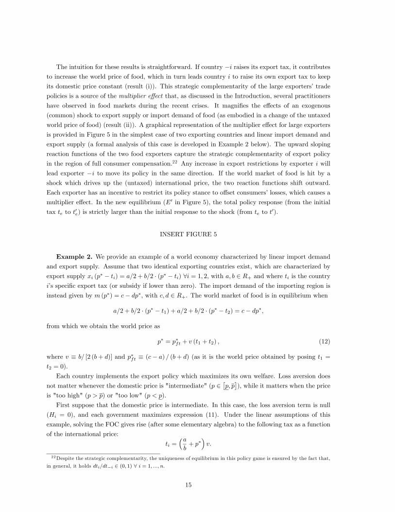
The intuition for these results is straightforward. If country −i raises its export tax, it contributesto increase the world price of food, which in turn leads country i to raise its own export tax to keep
its domestic price constant (result (i)). This strategic complementarity of the large exporters’trade
policies is a source of the multiplier effect that, as discussed in the Introduction, several practitioners
have observed in food markets during the recent crises. It magnifies the effects of an exogenous
(common) shock to export supply or import demand of food (as embodied in a change of the untaxed
world price of food) (result (ii)). A graphical representation of the multiplier effect for large exporters
is provided in Figure 5 in the simplest case of two exporting countries and linear import demand and
export supply (a formal analysis of this case is developed in Example 2 below). The upward sloping
reaction functions of the two food exporters capture the strategic complementarity of export policy
in the region of full consumer compensation.22 Any increase in export restrictions by exporter i will
lead exporter −i to move its policy in the same direction. If the world market of food is hit by ashock which drives up the (untaxed) international price, the two reaction functions shift outward.
Each exporter has an incentive to restrict its policy stance to offset consumers’losses, which causes a
multiplier effect. In the new equilibrium (E′ in Figure 5), the total policy response (from the initial
tax te to t′e) is strictly larger than the initial response to the shock (from te to t′).
INSERT FIGURE 5
Example 2. We provide an example of a world economy characterized by linear import demandand export supply. Assume that two identical exporting countries exist, which are characterized by
export supply xi (p∗ − ti) = a/2 + b/2 · (p∗ − ti) ∀i = 1, 2, with a, b ∈ R+ and where ti is the country
i’s specific export tax (or subsidy if lower than zero). The import demand of the importing region is
instead given by m (p∗) = c− dp∗, with c, d ∈ R+. The world market of food is in equilibrium when
a/2 + b/2 · (p∗ − t1) + a/2 + b/2 · (p∗ − t2) = c− dp∗,
from which we obtain the world price as
p∗ = p∗ft + v (t1 + t2) , (12)
where v ≡ b/ [2 (b+ d)] and p∗ft ≡ (c− a) / (b+ d) (as it is the world price obtained by posing t1 =
t2 = 0).
Each country implements the export policy which maximizes its own welfare. Loss aversion does
not matter whenever the domestic price is "intermediate" (p ∈[p, p]), while it matters when the price
is "too high" (p > p) or "too low" (p < p).
First suppose that the domestic price is intermediate. In this case, the loss aversion term is null
(Hi = 0), and each government maximizes expression (11). Under the linear assumptions of this
example, solving the FOC gives rise (after some elementary algebra) to the following tax as a function
of the international price:
ti =(ab
+ p∗)v.
22Despite the strategic complementarity, the uniqueness of equilibrium in this policy game is ensured by the fact that,
in general, it holds dti/dt−i ∈ (0, 1) ∀ i = 1, ..., n.
15
The reaction function of country i can then be simply found by substituting for (12) into this last
equation, thus obtaining
ti =v
1− v2
(ab
+ p∗ft + vt−i
).
Posing ti = t−i = t, the symmetric equilibrium tax policy is
t =v
1− 2v2
(ab
+ p∗ft
).
To characterize the upper region of compensating protection, we need to find the values of pft and
pcft. The value of pft is, by definition, the one such that the domestic price resulting from policy t be
equal to p, that is to say,
p∗(t, pft
)− t = p.
Exploiting our linear price function in (12) and substituting for the value of t found above, we can
solve for pft to obtain
pft =(1− 2v) ab + p
(1− 2v2
)1− v
If the world economy fundamentals are such that p∗ft < pft, then the equilibrium tax is t.
If p∗ft > pft instead, loss aversion matters, and each government maximizes expression (10). The
steps necessary to characterize pcft are analogous to those just taken to characterize pft.23 Since they
do not add any additional insight, we omit them and study the strategic interaction along this upper
region of compensating protection.
We know that, when p∗ft ∈(pft, p
cft
), each country i wants to keep its domestic price constant at
pi = p. Thus it poses ti = p∗ − p. The reaction function of country i can then be simply found bysubstituting for (12) into this last equation, thus obtaining
ti =p∗ft − p1− v +
v
1− v t−i.
Given that v ∈ (0, 1/2), it is immediate to prove that export taxes are strategic complements, that is
dtidt−i
=v
1− v > 0.
In a symmetric equilibrium it holds ti =
p∗ft−p1−v + v
1−v t−i
ti = t−i
from which we obtain the equilibrium tax as
t∗ =1
1− 2v
(p∗ft − p
)> 0.
Then it isdt∗
dp∗ft= Φ
∂t∗
∂p∗ft,
23The maximization of (10) gives rise to an export tax t, which is strictly higher than t. This allows us to find the
value of the free trade world price such that the domestic price resulting from the equilibrium policy be equal to p,
that is to say, that value of pcft such that p∗(t, pcft
)− t = p. To find the explicit value for pcft as a function of all the
parameters of the model however, we would further need to specify a functional form for both h (·) and for the utilityfunction u (·).
16
where the multiplier is given by
Φ ≡ 1
1− 2v> 1 as v <
1
2.
Of course, an analogous reasoning can be carried out to identify the lower region of compensating
protectionism, and to show the strategic complementarity of export policies and the existence of a
multiplier effect.
6 Discussion
The analysis so far is based on two main simplifying assumptions. First, governments maximize
national welfare. Second, importers do not alter their trade policy. This section discusses how our
central result of a multiplier effect in food export policy will be affected as we remove each of these
assumptions. The goal here is to guide the empirical analysis of the next section rather than providing
a complete analytical discussion.
6.1 Political economy
A large body of trade literature assumes that owners of specific factors are politically organized to
lobby the government, as they are generally more easily coalised into an interest group. In a political
economy context, it can be shown that governments weigh more heavily organized interests that, as
a result, receive favorable policies in the form of tariff protection or export subsidies (Grossman and
Helpman, 1994). The recent works by Freund and Ozden (2008) and Tovar (2009) show that this
result carries over to a situation where producers face loss aversion. Similarly, within the context of
our model, it is immediate to realize that, when the domestic price is "intermediate" (p ∈[p, p]), a
politically motivated government would set an export subsidy rather than free trade in response to
lobbying pressures by land owners. In addition, it can be shown that there is a first region of full
producer compensation when the price is low (below p), where the government sets an export subsidy
given by condition (6).24
When the domestic price is high (p > p), a politically motivated government faces a trade off
between political economy considerations and the loss aversion caused by high food prices. However,
it is easy to prove that there is a region of full consumer compensation where the loss aversion effect
is strong, and the government wants to keep the domestic price constant at p.25 Hence, while political
economy considerations bias trade policy towards the granting of export subsidies, a multiplier effect
of export policy would still result when the food price falls within the regions of full compensation.
24The proofs of these statements are omitted as they follow directly from Freund and Ozden (2008).25We only sketch the argument here, while a detailed proof is available from the authors upon request. Define the
political welfare of government as J = Ω +H, where H is defined as in Section 3, while Ω = bπ+CS +GR, with b > 1
representing the political bias. This can be interpreted as the reduced-form of a two stage lobbying game, as in Grossman
and Helpman (1994). Denote by s (p∗) the politically optimal subsidy when the domestic price is intermediate, that is,
when p = p∗ + s (p∗) ∈[p, p]. This domestic price is the one for which G′ = Ω′ = 0. When -as a result of an increase
in the world price p∗- the domestic price grows slightly above the upper threshold, say when p = p + ε, we have that
G′ = Ω′ + H′ > 0, as Ω′ = 0 but H′ > 0. For a range of ε small enough, the solution to this maximization problem
is a corner solution in which the government utilizes export policy to keep the domestic price constant at p = p. This
policy consists of gradually reducing the subsidy s (p∗) as p∗ grows large. When p∗ grows higher than p, the optimal
policy becomes an export tax.
17
6.2 Import policy
The model presented in this paper focuses on food exporters. However, importing countries may
respond to changes in international prices, which is likely to exacerbate situations of stress in in-
ternational food markets. First, a multiplier effect may arise in import as well as in export policy.
Assuming that preferences in importing countries are defined as in condition (1) and that there is
a continuum of identical small importers, it is possible to show that, similarly to the exporters in
our model, importing governments face incentives to use trade policy to insulate their domestic food
market. Specifically, for a given export policy, there are regions of full compensation where the ob-
jective of trade policy is to preserve the level of the domestic price of food. When prices are high,
importers provide food import subsidies or lower trade barriers; while the response to a low price is
the imposition of tariffs on food products or lower subsidies to imports. As all importers face exactly
the same incentives and act simultaneously, their trade policy affects the international price of food,
creating a multiplier effect similar to the one discussed earlier for exporters.
Second, and more importantly, as discussed in Anderson and Martin (2011) and Bouet and Laborde
(2011), the interaction between exporters on the one hand and importers on the other magnify sit-
uations of stress in world food markets. Specifically, if world food prices are high, both exporters
and importers set trade policy to shield the domestic market from developments in the international
market. However, the joint imposition of higher export taxes and lower import tariffs (or higher
import subsidies) contracts world supply and expands world demand, thus resulting in even higher
international food prices.26
7 Export policy and the 2008-10 food crisis
In this section, we test empirically the validity of the model. Specifically, we examine whether the
pattern of export policies that countries implement during periods in which prices move away from
their reference point is consistent with our theoretical predictions. As a first step, we test whether
export measures are related with changes in international food prices. We then examine whether
exporting countries use trade intervention as a response to policies implemented by other governments.
As seen in Sections 4 and 5, this behavior gives rise to an export policy multiplier effect and thus
determines an equilibrium where world food prices are pushed further away from their free trade level.
We then tackle the issue of endogeneity of our two key variables (export policies and prices) to verify
the robustness of our empirical findings. In the final part of this section, we evaluate the impact of
overall export policy changes on international prices. Given the two-way relationship between export
policies and world prices, we do this by estimating a system of simultaneous equations.
The focus of our analysis is the time period 2008-2010, which is characterized by high food and
other commodity prices.27 During this period, food prices were almost 60 per cent higher than average
26 In terms of Figure 4, changes in import policy can be captured by shifts to the right of the international price
line p∗(t). Clearly, increases on the international price of food are a terms-of-trade gain for exporting countries and a
terms-of-trade loss for importing countries. This simple observation supports the view that in a food crisis net importers
have more to lose compared to net exporters of food.27When the data were collected, detailed information on export policy, our main variable of interest, was only available
for these three years (see Section 7.1).
18
prices during the period 1990-2006. This surge in prices has been particularly strong in some sectors,
namely staple foods such as cereals, where the increase in average prices was higher than 90 per cent.
Also price volatility has been significantly high during the last three years compared with 1990-2006
(see Table 1). These figures allow us to assume that during 2008-2010, prices were above their reference
level p for the set of food products considered in the study. This is a convenient simplification, since it
allows us to undertake the analysis without having to identify the precise reference price for different
products, which is not always an easy task. Finally, we focus on the universe of export restrictions
rather than export subsidies.28 This is because, consistently with the theory, during periods of high
international food prices countries tend to use export restrictions to insulate the domestic market.
INSERT TABLE 1
7.1 Data
Data on export and import policy implementation comes from two different sources: the WTO Trade
Monitoring Reports (TMR) and from the Global Trade Alert (GTA) database. The main objective of
the WTO monitoring reports is to increase the transparency and understanding of the trade policies
and practices of member countries affecting the multilateral trading system. Specifically, the mon-
itoring reports of October 2009, November 2010 and March 2011 provide information on the type
and the status of trade-related measures that have been implemented by governments after the 2008
global financial crisis. These measures have been notified by WTO members and observer govern-
ments to the secretariat of the WTO. Our second source, the Global Trade Alert, is an independent
monitoring exercise of policies that affect global trade. The GTA database not only includes informa-
tion on discriminatory measures provided by governments, but it also contains information collected
from exporters, the media and trade analysts. An evaluation group composed by expert analysts is
responsible for assessing this information and deciding whether to publish it on the website.
A total of 85 export restrictions have been recorded in food products during the time period 2008-
2010.29 The share of trade that is covered by these restrictions significantly varies across products. For
commodities such as palm oil and cocoa, the amount of trade covered by export restrictive policies
is equal to 50 and 47 per cent respectively. In the case of staple products such as cereals, which
constitute a dominant part of consumers’diet especially in low income countries, the share of trade
covered by export restrictions is also significant, ranging from 14 per cent in the case of wheat and
meslin to almost 35 per cent in the case of rice. Details are provided in Table 2.
INSERT TABLE 228A similar exercise could, in principle, be done with export subsidies for periods where international food prices were
historically low and presented a downward trend, such as in the second half of the 1980s.29This figure is likely to underestimate the effective number of export measures that have been implemented. The
reason is that export restrictions recorded in each month often include more than a single measure. Our data sets,
however, do not allow us to precisely discern this information.
19
With respect to the type of export measures implemented by countries, almost half of the restric-
tions are export prohibitions, 24 per cent are either an imposition or an increase in an existent export
tax and 10 per cent are export quotas and licensing. The remainder is represented by other measures
such as price references or technical requirements (see Table 3). The pattern in the type of export
measures implemented by countries for staple foods is very similar to those used in the food sector as
a whole.
INSERT TABLE 3
The rest of the data are from standard sources. International nominal prices come from the FAO
and IMF databases. Data on production shares are also taken from FAO. The share of agricultural
value added is collected for 2009 and comes from the World Development Indicators. Data on total
exports come from UN Comtrade and from the Global Trade Atlas database.
7.2 Determinants of export policy
To analyze the impact of international prices and overall export policies on the probability of impos-
ing an export restriction, we regress the following specification using monthly data for a set of 125
exporting countries and 29 commodity products:
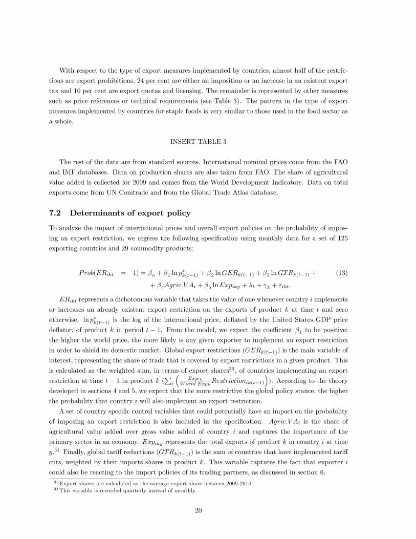
Prob(ERikt = 1) = βo + β1 ln p∗k(t−1) + β2 lnGERk(t−1) + β3 lnGTRk(t−1) + (13)
+ β4Agric.V Ai + β5 lnExpiky + λt + γk + εikt.
ERikt represents a dichotomous variable that takes the value of one whenever country i implements
or increases an already existent export restriction on the exports of product k at time t and zero
otherwise. ln p∗k(t−1) is the log of the international price, deflated by the United States GDP price
deflator, of product k in period t − 1. From the model, we expect the coeffi cient β1 to be positive:
the higher the world price, the more likely is any given exporter to implement an export restriction
in order to shield its domestic market. Global export restrictions (GERk(t−1)) is the main variable of
interest, representing the share of trade that is covered by export restrictions in a given product. This
is calculated as the weighted sum, in terms of export shares30 , of countries implementing an export
restriction at time t− 1 in product k (∑
i
(Expik
World ExpkRestrictionik(t−1)
)). According to the theory
developed in sections 4 and 5, we expect that the more restrictive the global policy stance, the higher
the probability that country i will also implement an export restriction.
A set of country specific control variables that could potentially have an impact on the probability
of imposing an export restriction is also included in the specification. Agric.V Ai is the share of
agricultural value added over gross value added of country i and captures the importance of the
primary sector in an economy. Expiky represents the total exports of product k in country i at time
y.31 Finally, global tariff reductions (GTRk(t−1)) is the sum of countries that have implemented tariff
cuts, weighted by their imports shares in product k. This variable captures the fact that exporter i
could also be reacting to the import policies of its trading partners, as discussed in section 6.30Export shares are calculated as the average export share between 2009-2010.31This variable is recorded quarterly instead of monthly.
20
7.2.1 Baseline regression results
The outcomes from regression (13) are reported in Table 4. The estimations are performed using both
a logit model and a linear probability model (LPM). We undertake the analysis for all food products
in our dataset (columns (1) to (6)) and for a sub-set of staple food products (columns (7) to (9)).32
In the regressions we also include 4-digit product and time (month) fixed effects in order to control
for product and time specific characteristics, and we cluster standard errors at country level to take
into account the fact that the observations in the variables of our main interest (international prices
and policies) are not independent across countries. The estimations of the linear probability model
are also performed including country fixed effects.33
INSERT TABLE 4
From columns (1)-(3) we can observe that increases in international prices have a positive and
significant impact on the probability of implementing an export restriction. In the regressions that
include all the 29 food products in our sample, the size of the coeffi cient is however rather small. A
100 per cent surge in international prices in t − 1 increases the probability of imposing an export
restriction in t by 0.1 per cent. Results are different for staple food products. From column (7) it is
possible to see that the impact of international prices is forty times higher for staple foods compared
to the whole food sector. Specifically, a 100 per cent surge in international prices in t − 1 increases
the probability of imposing an export restriction in t by 4 per cent. This is not surprising given that
staple products represent an important component of total food consumption, therefore governments
(in line with the spirit of our model) tend to use export policy for products where consumers’losses
are more significant.
In columns (4)-(6), we look at the impact of export and import policies on the probability of
imposing an export restriction. A positive and significant coeffi cient of the variable capturing the
global level of export restrictions confirms that governments impose these measures in reaction to
the restrictive policy imposed by other exporters. Specifically, in the logit model, a 100 per cent
increase in the share of trade covered by export restrictions on a product raises the probability of
imposing a new trade restricting policy on that product by 2 per cent on average and by 4 per cent
for staple food products (see column (4) and (8) respectively). The coeffi cient is still positive and
significant when a linear probability model is estimated (see columns (5) and (6)). Interestingly, once
global restrictions are introduced in the regression, the coeffi cient on the price becomes smaller and, in
some specifications, loses significance. This is compatible with the prediction of the theoretical model
that new restrictive measures are mostly driven by other export restrictions. Finally, the coeffi cient
capturing the global level of import restrictions is never significant. This result is in contrast with
studies such as Anderson and Martin (2011) and Bouet and Laborde (2011) which show that the
interaction between exporting and importing countries should lead to further increases in international
32Specifically, we consider the following products: grain, weath and meslin, maize, barley and rice. For simplicity, only
the logit regressions results are included in Table 4 -results using a LPM are very similar and available upon request.33 In the logit model country fixed effects are excluded from the estimation. This in order to be able to include in the
regression a control group of countries that have never imposed an export restriction.
21
prices and even more stringent export policies. One possible explanation is that in our dataset, the
share of trade covered by import reducing barriers is not very large (less than 2 per cent). This
indicates that importing countries react through measures other than tariffs, such as import subsidies
or other domestic instruments (for which, however, data are not available).
The coeffi cients of the country specific control variables all have the expected sign. β5 is positive
and significant, implying that countries with higher levels of exports of a product are more inclined
to impose an export restriction. We come back to this point below. Also β4 is positive and significant
suggesting that the higher the share of agriculture on gross value added of a country, the higher
the probability of imposing an export restriction. Economies that have a higher dependency on the
production of primary products are typically low income countries. During periods of high food prices,
there are two reasons why these countries may be more inclined to impose export restrictions. First,
people in low income economies spend a higher shares of their income on food. Second, these countries
generally have a limited number of domestic policy instruments available to protect consumers from
an increase in domestic food prices.
7.2.2 Are large exporters different?
Next we investigate whether larger exporters are more likely to impose an export restriction when
international prices are increasing or as a reaction to other countries’export restrictions. In order to
do this, we introduce two interaction terms in the baseline regression: the first between large exporters
and the level of international prices; the second between large exporters and the global level of export
restrictions. The term representing large exporters is captured by a dichotomous variable equal to
one if the share of country i’s exports over world exports of a certain product k is greater than 10 per
cent.34
The results are presented in Table 5. Columns (1) and (2) show the impact of being a large exporter
on the probability of imposing an export restriction. The first regression includes as a control variable
the level of quarterly exports. The coeffi cient on the large exporter dummy is positive in both cases
and significant only in the latter case, due to high correlation between this variable and the quarterly
level of exports. As predicted by the theory, countries with contractual power in export markets
are more likely to impose an export restriction to exploit terms of trade effects. In columns (3) and
(4) the interaction term between large exporters and international prices is included. A positive and
significant coeffi cient for this term confirms that larger exporters are more likely to react to increases in
international prices than smaller exporters. When the global level of export restrictions is introduced
in the regression, the effect of international prices for small exporters becomes insignificant, while the
interaction between international prices and large exporters is still significant (see columns (5) and
(6)).
INSERT TABLE 5
The interaction term between large exporters and the global level of export restrictions is intro-
duced in the last two columns of Table 5. The effect of global export restrictions on the probability of34Regressions are also performed considering as large exporters those countries whose share of world exports is higher
than 5 per cent. The results presented below still hold.
22
imposing a new restrictive measure is magnified for large exporters of food. Once this interaction term
is introduced in the regression, the coeffi cient on the variable measuring global restrictions in a prod-
uct loses significance. This suggests that the multiplier effect of export policy is driven by actions of
large exporters, whose policies are strategic complements along the region of consumer compensation.
The prominence of large exporters may also contribute to explain why the coeffi cients in the baseline
regressions (while significant and with the expected sign) are relatively small. In the food sector, large
exporters of a certain food product tend to be also large consumers of that good. Therefore, most
of the effects described in our model are likely to be present for large exporters/consumers. Many
small exporting countries are inactive simply because they also consume very little of the food product
they export. For this reason, these countries generally have a small incentive to intervene to offset
consumer losses (the main exception being for staple foods where, in fact, coeffi cients were larger).
7.2.3 Endogeneity
A possible concern with the previous estimations is that international prices and global restrictions
are likely to be endogenous due to the presence of simultaneity bias (as we found in the theoretical
model). To deal with this problem we use two different strategies.
First, we perform our regressions increasing the number of lags in the independent variables of our
interest. Specifically, estimations are performed calculating international prices and the global level
of export policy restrictions in t − 2 and t − 3 respectively for both the broader sample of all food
products and the sub-set of staple foods. The results, presented in Appendix Table C1, show that the
magnitudes of the impact of international prices and of the global level of export restrictions on the
probability of imposing a new restrictive measure are very similar to the ones in our baseline regressions
(Table 4). In addition, we interact the dichotomous variable capturing large exporters with the lagged
international prices and the lagged global export restrictions. The results in Appendix Table C2 are,
once more, very similar to the findings in Table 5.35
As a second strategy to address the endogeneity bias, we follow an instrumental variables ap-
proach to estimate specification (13). For the international price variable we generate two different
instruments based on climatic conditions, which have a direct impact on the total production of food
products and, therefore, affect their prices in international markets through the supply channel. The
first instrument Rainkt measures the total level of rainfalls taking place in the top 5 producer countries
of a certain product k at time t.36 The second instrument, Rainvarkt, captures the total variability
of rainfalls in the top 5 producer countries of a certain product k at time t.37 The results from the
first stage regression of the IV specification, presented in columns (1) and (2) of Appendix Table C3,
suggest that rainfall is a good predictor for the international prices variable. High levels of rainfall
are negatively correlated with crops production. In addition, the higher the number of top producers
experiencing levels of rainfall that highly deviate from their historical mean, the higher the negative
impact on total production.
35Note that the variable log of quarterly exports has been excluded from the regression since it is sometimes collinear
with the variable big exporter.36Alternative instruments have been created considering the top 3 and the top 10 producers of a product. Results do
not change significantly.37This instrument is computed as the total count of top producers for which the amount of rain in a certain month
has been either above the 85th percentile or below the 25th percentile compared to its historical mean.
23
For the overall level of export restrictions existent in a product k we use two instruments. The
first instrument, Electionskt, is a variable that indicates whether there will be elections taking place
in the next three months in the top five producer countries. As discussed in Section 6, lobby groups
representing producers’ interests will generally oppose the imposition of an export restriction. In
the proximity of elections, governments may be more willing to cede to requests from these special
interests and, hence, are less likely to impose a restrictive export measure. As a second instrument,
we use the total number of restrictions that have been applied in the two-digit industry to which the
product belongs (ER−kt =∑
i
∑j 6=k Exp restrictionijt). During periods of increasing food prices,
countries might react to the fact that international markets are getting more restrictive by imposing
an export restriction themselves. This may be the result of a sort of "simulation effect" or may occur
because countries expect increasing prices in product k deriving from shifts in international demand
caused by restrictions in other products. The first stage results for the IV specification confirm a
negative correlation between the global level of export restrictions in a product and the variable
capturing elections in large producing countries (the first instrument) and a positive correlation with
the number of export restrictions in the corresponding industry (the second instrument). In addition,
the F-statistic of the regression indicates that none of the instruments are weak (see columns (2) and
(3) of Appendix Table C3).
Second stage regression results are presented in Table 6. The first two columns are introduced for
comparison and simply report the coeffi cients of the two main variables of interest (international prices
and global export restrictions) for the baseline regressions on the entire sample and for the sub-set of
large exporters. Columns (3) to (6) report results of the IV regressions.38 Global export restrictions
are still found to have a positive and significant impact on the probability of imposing a new restrictive
policy. As in the baseline regression, the coeffi cient on international prices is significant if introduced
alone in the regression and loses significance once global restrictions are included as an explanatory
variable, compatibly with the theoretical prediction that restrictive export policy is driven by the
choices of other exporters. In the last two columns of Table 6, regressions are computed for large
exporters only. Results confirm that the multiplier effect is especially strong for big food exporters.
Finally, note that the magnitudes of the coeffi cients capturing global restrictions in the IV regressions
are in line with the ones of the baseline regressions reported in columns (1) and (2).
INSERT TABLE 6
7.3 Impact of export restrictions on food prices
The empirical analysis so far has shown that exporters set trade policy in response to developments
in international food markets, as captured by the world price of food, and -more importantly- that
they react to the trade policy chosen by other exporters. As we discussed, this evidence is compatible
with the existence of a multiplier effect in food export policy. A compelling, but rather diffi cult,
issue is to assess the overall impact that changes in export policy had on international food prices
38Regressions have also been estimated computing the instruments for international food prices and global export
restrictions lagged by one period. Results still hold.
24
during the 2008-10 food crisis. The diffi culty lies in the fact that export policy is endogenous. As
shown in the theoretical models of Sections 4 and 5, changes in export policy may be induced by
increases in international food prices, which in turn are affected by trade policy changes. To deal with
this endogeneity, we use a two-stage least squares (2SLS) approach in order to estimate the following
system of simultaneous equations consistent with our theoretical model:
ln p∗kt = α0 + α1 lnGERkt + α2 lnRainkt + α3 lnRainvarkt + α4 lnEnergyt + γk + λt + εkt
lnGERkt = β0 + β1 ln p∗kt + β2 lnElectionskt + λt + γk + ukt.
The first equation of the system is the one of our interest and represents the level of the world
price of product k as a function of global export restrictions. We expect that global restrictions
imposed on product k will have a positive impact on its international price. In the specification, we
introduce a set of time-varying control variables that could potentially affect the international price.
These variables include the total level and the variability of rainfalls in the top producer countries (as
defined in Subsection 7.2.3) and the level of energy prices. Finally, γk and λt are a set of product and
time fixed effects. The second equation of the system represents global export restrictions on product
k. This variable depends on the level of international prices, because increases in the price of product
k are expected to induce exporting governments to use trade policy to address consumers’losses. As
additional explanatory variable in the regression, we include the instrument measuring the proximity
of elections in top producing countries.
The second stage results are presented in Table 7 and provide further evidence of the existence
of a multiplier effect of export policy in the food sector. The regressions are performed using the
entire sample of 29 food products. Global export restrictions in a certain product k have a positive
and significant impact on the international prices of that product. Specifically, an increase by 1 per
cent in the share of trade covered by export restrictions, raises international prices by 1.1 per cent on
average. While this effect is sizeable, this is likely to be a "conservative" estimate of the impact that
export restrictions had on food prices during 2008-10. The reason is that this coeffi cient averages out
products such as staple foods, where policy makers were shown to be more prone to impose restrictions
in response to other countries’export restraints, and products where the multiplier effect was found
to be less relevant. While the presumption is that the coeffi cients would be even higher if we were
to perform the regression only for the sub-set of staple food products, where shares of trade covered
by export restrictions ranged between 14 per cent and 35 per cent, the data are too limited to obtain
statistically meaningful results using this methodology.
INSERT TABLE 7
8 Conclusions and policy implications
In his essay "Of the Balance of Trade", David Hume wrote:
25
"It is very usual, in nations ignorant of the nature of commerce, to prohibit the exportation
of commodities, and to preserve among themselves whatever they think valuable and useful.
They do not consider, that, in this prohibition, they act directly contrary to their intention
... To this day, in France, the exportation of corn is almost always prohibited; in order,
as they say, to prevent famines; though it is evident, that nothing contributes more to the
frequent famines, which so much distress that fertile country." (Hume, 1742).
As this quote reminds us, economists have for long time believed that a link exists between re-
strictive export policy and food crises. This paper fits in this tradition by presenting a model of food
export policy when agents are averse to losses. The theory predicts a pattern of trade policy that is
broadly consistent with observed behavior. Specifically, exporting governments offer export subsidies
when food prices are low and set export restrictions when prices are high. Moreover, the theory for-
malizes a significant channel through which these policy actions can destabilize global food markets.
This results from a multiplier effect, similar to the concept familiar in macroeconomic theory, where
world food price changes feed into increasingly export policy activism.
We test empirically the theory by looking at the period of high food prices of 2008-10. In particular,
we study two predictions of the model. First, exporting countries set restrictions in response to
restrictive measures imposed by other food exporters. Second, export policy impacts on international
food prices. In the empirical analysis we employ a novel dataset that contains detailed information
on trade policy choices taken by exporting governments. Our results confirm that changes in export
policy are set in response to restrictions imposed by other exporters, particularly for large exporters
and in important products such as staple foods. Moreover, the overall impact of these measures has
been to significantly increase food prices in 2008-10.
This multiplier mechanism in food markets bears consequences for global welfare. An increase
(fall) in the world price of food is a terms of trade gain (loss) for exporting countries and a terms
of trade loss (gain) for importers. While these effects cancel each other out, export policy activism
creates the traditional distortions and deadweight loss that lower global welfare. The interests of
exporters and importers are, however, not aligned: the negative welfare effect of an escalation of
export restrictions (subsidies) will fall on food importing (exporting) countries. This fact makes any
policy reform diffi cult. In addition to these welfare consequences, the multiplier effect may also have
an adverse impact on welfare through its effect on short-run volatility in food prices. A formal analysis
of this aspect is beyond the scope of the present study, but it represents an interesting avenue for
future research.
Several academic studies and a report by a number of international organizations have recently
addressed the effi ciency of multilateral trade rules in the wake of the recent food crises and discussed
avenues for improvements.39 We see the present work as a contribution to this broader debate. WTO
rules on export policy are characterized by two asymmetries. Differently from industrial products, ex-
port subsidies for agricultural goods are not prohibited under WTO rules. However, in the Uruguay
Round Agreement on Agriculture signed in 1995, member governments from developed countries
39See FAO et al. (2011). The report proposes to eliminate export subsidies, limit the applicability of food bans and
improve the notification requirement for food export restrictions. The report also includes a number of proposals to
improve policy tools directly targeting losses arising from changes in food prices.
26
agreed to introduce in the multilateral trading system commitments to bind agricultural export sub-
sidies. In the context of the on-going Doha negotiations, member countries are discussing further
restraints on their food subsidy policy. While the adequacy (i.e. the depth and width) of existing
commitments can be debated, the logic of the agreement appears to be consistent with the need to
address an export subsidy multiplier effect.40 The model also explains why the value of this reform is
likely to be more relevant than what is perceived at times, as the current one, when high food prices
have greatly reduced the use of export subsidies. This is precisely because, if world prices were to
fall again in the future, the incentive to apply export support measures in this sector would certainly
re-emerge, along with the associated multiplier mechanism.
A second asymmetry in WTO rules is that the regulation of export restrictions is weaker than
the disciplines on export promotion. Under WTO rules, members are prohibited from instituting or
maintaining quantitative restrictions, but exceptions (subject to specific requirements) are allowed in
food sectors. In addition, export taxes are loosely regulated and are, in general, not covered by binding
commitments. This implies that there are no export duties ceiling rates and no limitations regarding
the timeframe for applying or increasing an export tax. Overall, this legal framework generally gives
WTO members a significant discretionary scope in applying export restrictions. The results presented
in this paper, however, suggest that this flexibility may adversely affect global welfare, as unilateral
export restrictions in times of high food prices create a multiplier effect that pushes prices further
up. The introduction of commitments in export policy, for instance in the form of negotiated export
tax bindings, would smooth this impact, both directly and by inducing countries to develop more
targeted policy instruments to protect consumer losses, rather than relying on second-best trade
policy intervention.
References
[1] Aksoy, M.A. and B.M. Hoekman (2011). "Food Prices and Poverty: Introduction and Overview".
In Aksoy and Hoekman eds. Food Prices and Poverty. World Bank.
[2] Anderson, K. and W. Martin (2011). "Export Restrictions and Price Insulation during Commod-
ity Price Booms". World Bank Policy Research Working Paper No. 5645.
[3] Bagwell, K. and R.W. Staiger (2001). "Strategic Trade, Competitive Industries and Agricultural
Trade Disputes". Economics and Politics, 13: 113-28.
[4] Bagwell, K. and R.W. Staiger (2002). The Economics of the World Trading System. MIT Press,
Cambridge.
40 In the chapter dedicated to export subsidies, Bagwell and Staiger (2002, ch. 10) note that rules that facilitate a
reduction in trade volume warrant special scrutiny. Their argument being that, differently from export restrictions,
export subsidies have a positive effect on welfare of importing countries via a terms-of-trade change. While this argument
is clearly correct, it is softened by the theory presented here. The reason is that, as the model and recent experience
show, exporting governments recur to subsidies when the world price of food is low while imposing restrictions when the
price is high. Therefore the positive terms-of-trade effect of subsidies hits when it is, so to say, less needed by importers.
27
[5] Bouet, A. and G. Laborde (2010). "Economics of Export Taxation in the Context of food Crisis:
A Theoretical and CGE Approach Contribution". International Food Policy Research Institute,
Discussion Paper No. 00994.
[6] Broda, C., D. Weinstein and N. Limao (2008). “Optimal Tariffs and Market Power: The Evi-
dence.”American Economic Review, 98(5), pp. 2032-65
[7] Camerer, C. (1995). "Individual decision making", in Handbook of Experimental Economics, ed.
by A. R. J. Kagel, Princeton University Press, vol. 2.
[8] Chauffour, J.P. (2008). "Global Food Price Crisis: Trade Policy Origins and Options". PREM
Trade Note No. 119. World Bank.
[9] Cooper, R. and A. John (1988). "Coordinating Coordination Failures in Keynesian Models".
Quarterly Journal of Economics, 103 (3), pp. 441-63.
[10] Deaton, A. and G. Laroque (1992). "On the Behaviour of Commodity Prices". Review of Eco-
nomic Studies, 59:1, 1-23.
[11] FAO, IFAD, IFPRI, IMF, OECD, UNCTAD, WFP, World Bank, WTO, UN HLTF (2011). Price
Volatility in Food and Agricultural Markets: Policy Responses. Policy Report for the G-20. May,
2011.
[12] Freund, C. and C. Ozden (2008). "Trade Policy and Loss Aversion". American Economic Review,
98:4, 1675-91.
[13] Gouel C. and S. Jean (2012). "Optimal food price stabilization in a small open developing coun-
try". Policy Research Working Paper 5943, The World Bank.
[14] Grossman, G.M. and E. Helpman (1994). "Protection for Sale". American Economic Review,
84:4, 833-850.
[15] Headey, D. (2011). "Rethinking the Global Food Crisis: The Role of Trade Shocks". Food Policy,
36, 136-46.
[16] Hochman, G., D. Rajagopal, G. Timilsina, and D. Zilberman (2011). “Quantifying the causes of
the global food commodity price crisis”, World Bank working paper, forthcoming.
[17] Hume, D. (1742). "Of the Balance of Trade". Reprinted in Essays: Moral, Political and Literary.
Liberty Fund, Indianapolis.
[18] Ivanic, M., Martin W. and A. Mattoo (2011). "Welfare and Price Impacts of Price Insulating
Policies". Mimeo, World Bank.
[19] Kahneman, D. and A. Tversky (1979). "Prospect theory: an analysis of choice under risk",
Econometrica, 47, 263-291.
[20] Koszegi, B. and M. Rabin (2006). "A Model of Reference-Dependent Preferences", Quarterly
Journal of Economics, 121, 1133-1165.
28
[21] Lamy, P. (2011a). "More Trade, Less Hunger". Project Syndicate, February 21st, 2011.
[22] Lamy, P. (2011b). "International Trade -A Vital Component of the Food Security Picture".
Opening Address at the XIII Congress of the European Association of Agricultural Economists.
August, 2011.
[23] Limao, N. and K. Saggi (2011). "Size Inequality, Coordination Externalities and International
Trade Agreements". Mimeo. University of Maryland.
[24] Limao, N. and P. Tovar (2009). "Policy Choice: Theory and Evidence from Commitment via
International Trade Agreements". NBER Working Paper No. 14655.
[25] Piermartini, R. (2004). "The Role of Export Taxes in the Field of Primary Commodities". WTO
Discussion Paper. Geneva, World Trade Organization.
[26] Samuelson, W. and R. Zeckhauser (1988). "Status quo bias in decision making", Journal of Risk
and Uncertainty, 1, 7-59.
[27] Tovar, P. (2009). "The Effects of Loss Aversion on Trade Policy: Theory and Evidence". Journal
of International Economics, 78, 154-67.
[28] Tversky, A. and D. Kahneman (1981). "The framing of decisions and the psychology of choice,"
Science, 211, 453-458.
[29] Tversky, A. and D. Kahneman (1991). "Loss Aversion in Riskless Choice: A Reference-Dependent
Model", Quarterly Journal of Economics, 106, 1039-1061.
29
A The optimal export policy under inequality aversion
Consider a small open economy with an identical structure as the one described in Section 2, except
for two features. The first feature is that consumers are standard rational agents, that is, they are
not loss averse. Hence, I l = IL = 0, and the sum of land-owners’indirect utility can be expressed as
VL (p) = π (p) + α [CS (p) +GR (p)] ,
while the sum of workers’indirect utility is given by
Vl (p) = (1− α) [1 + CS (p) +GR (p)] .
The second feature is that the government is assumed to be averse to inequality. The simplest way
to capture government’s inequality aversion is by defining social welfare as
G (p) = h (VL (p)) + h (Vl (p))
where function h (·) is twice continuously differentiable with h′ (·) > 0, h′′ (·) < 0. Function h (·) ismeant to capture the idea that, coeteris paribus, a more equitable distribution of resources across
workers and land-owners is welfare enhancing.
Government’s objective is the one of finding price p, and hence tax/subsidy t = −s = p∗−p, whichmaximizes social welfare. From the FOC we obtain
dG
dp= (p∗ − p)x′ (p) [h′l (1− α) + h′Lα]− (1− α) y (p) (h′l − h′L) = 0,
where
h′l ≡dh
dVl, h′L ≡
dh
dVL.
After a few algebraic steps we can finally express the optimal tax/subsidy as
σ =t
p∗ − t =(1− α) (h′l − h′L)
(1− α)h′l + αh′L
z (p)
e (p), (14)
where z (p) ≡ y (p) /x (p), e (p) ≡ x′ (p) p/x (p).
The optimal policy is the one which optimally trades off the usual marginal loss caused by the
deviation from free trade with the marginal gain associated with a more equitable society. In par-
ticular, the optimal policy is a tax if and only if h′l > h′L, that is, if the marginal contribution of
workers’utility to social welfare is strictly higher than the one of land-owners, while it is a subsidy in
the opposite case. Only when h′L = h′l (which happens when workers and land-owners reach the same
level of welfare), the optimal policy is free trade.
Moreover, and crucially for our purpose, it is possible to prove that the optimal export tax (sub-
sidy), given by expression (14), is an increasing (decreasing) function of international food price p∗.41
41Define the "non-standard" part of the formula for the optimal export policy in (14) as
H ≡(1− α)
(h′l − h′L
)(1− α)h′l + αh′L
,
It is possible to prove that dH/dp∗ < 0 to the extent that h′′l , h′′L < 0 (that is, to the extent that the government is
inequality averse). The rest of the proof follows from the previous literature on trade policy (Grossman and Helpman,
1994, Freund and Ozden, 2008).
30
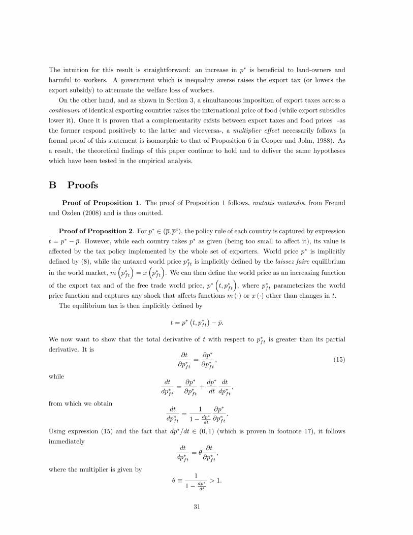
The intuition for this result is straightforward: an increase in p∗ is beneficial to land-owners and
harmful to workers. A government which is inequality averse raises the export tax (or lowers the
export subsidy) to attenuate the welfare loss of workers.
On the other hand, and as shown in Section 3, a simultaneous imposition of export taxes across a
continuum of identical exporting countries raises the international price of food (while export subsidies
lower it). Once it is proven that a complementarity exists between export taxes and food prices -as
the former respond positively to the latter and viceversa-, a multiplier effect necessarily follows (a
formal proof of this statement is isomorphic to that of Proposition 6 in Cooper and John, 1988). As
a result, the theoretical findings of this paper continue to hold and to deliver the same hypotheses
which have been tested in the empirical analysis.
B Proofs
Proof of Proposition 1. The proof of Proposition 1 follows, mutatis mutandis, from Freund
and Ozden (2008) and is thus omitted.
Proof of Proposition 2. For p∗ ∈ (p, pc), the policy rule of each country is captured by expression
t = p∗ − p. However, while each country takes p∗ as given (being too small to affect it), its value isaffected by the tax policy implemented by the whole set of exporters. World price p∗ is implicitly
defined by (8), while the untaxed world price p∗ft is implicitly defined by the laissez faire equilibrium
in the world market, m(p∗ft
)= x
(p∗ft
). We can then define the world price as an increasing function
of the export tax and of the free trade world price, p∗(t, p∗ft
), where p∗ft parameterizes the world
price function and captures any shock that affects functions m (·) or x (·) other than changes in t.The equilibrium tax is then implicitly defined by
t = p∗(t, p∗ft
)− p.
We now want to show that the total derivative of t with respect to p∗ft is greater than its partial
derivative. It is∂t
∂p∗ft=
∂p∗
∂p∗ft, (15)
whiledt
dp∗ft=
∂p∗
∂p∗ft+dp∗
dt
dt
dp∗ft,
from which we obtaindt
dp∗ft=
1
1− dp∗
dt
∂p∗
∂p∗ft.
Using expression (15) and the fact that dp∗/dt ∈ (0, 1) (which is proven in footnote 17), it follows
immediatelydt
dp∗ft= θ
∂t
∂p∗ft,
where the multiplier is given by
θ ≡ 1
1− dp∗
dt
> 1.
31
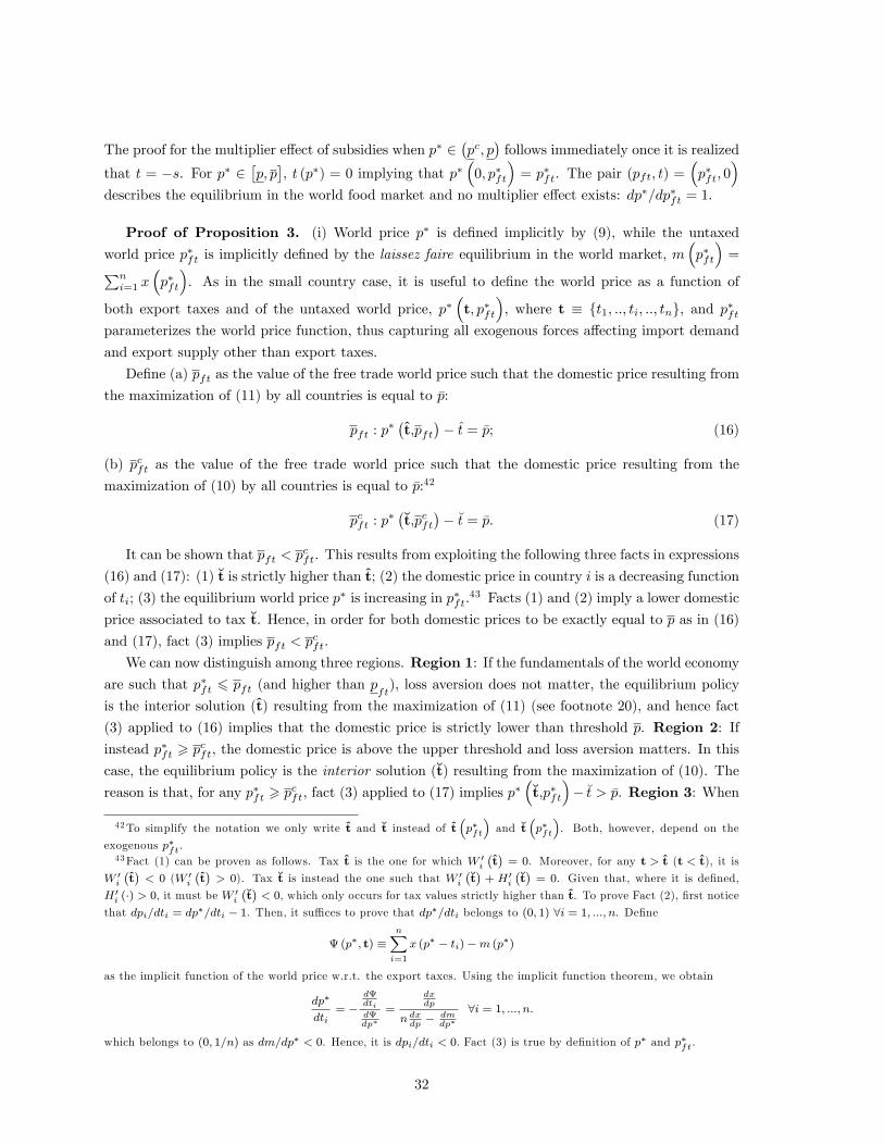
The proof for the multiplier effect of subsidies when p∗ ∈(pc, p
)follows immediately once it is realized
that t = −s. For p∗ ∈[p, p], t (p∗) = 0 implying that p∗
(0, p∗ft
)= p∗ft. The pair (pft, t) =
(p∗ft, 0
)describes the equilibrium in the world food market and no multiplier effect exists: dp∗/dp∗ft = 1.
Proof of Proposition 3. (i) World price p∗ is defined implicitly by (9), while the untaxed
world price p∗ft is implicitly defined by the laissez faire equilibrium in the world market, m(p∗ft
)=∑n
i=1 x(p∗ft
). As in the small country case, it is useful to define the world price as a function of
both export taxes and of the untaxed world price, p∗(t, p∗ft
), where t ≡ t1, .., ti, .., tn, and p∗ft
parameterizes the world price function, thus capturing all exogenous forces affecting import demand
and export supply other than export taxes.
Define (a) pft as the value of the free trade world price such that the domestic price resulting from
the maximization of (11) by all countries is equal to p:
pft : p∗(t,pft
)− t = p; (16)
(b) pcft as the value of the free trade world price such that the domestic price resulting from the
maximization of (10) by all countries is equal to p:42
pcft : p∗(t,pcft
)− t = p. (17)
It can be shown that pft < pcft. This results from exploiting the following three facts in expressions
(16) and (17): (1) t is strictly higher than t; (2) the domestic price in country i is a decreasing function
of ti; (3) the equilibrium world price p∗ is increasing in p∗ft.43 Facts (1) and (2) imply a lower domestic
price associated to tax t. Hence, in order for both domestic prices to be exactly equal to p as in (16)
and (17), fact (3) implies pft < pcft.
We can now distinguish among three regions. Region 1: If the fundamentals of the world economyare such that p∗ft 6 pft (and higher than pft), loss aversion does not matter, the equilibrium policy
is the interior solution (t) resulting from the maximization of (11) (see footnote 20), and hence fact
(3) applied to (16) implies that the domestic price is strictly lower than threshold p. Region 2: Ifinstead p∗ft > pcft, the domestic price is above the upper threshold and loss aversion matters. In this
case, the equilibrium policy is the interior solution (t) resulting from the maximization of (10). The
reason is that, for any p∗ft > pcft, fact (3) applied to (17) implies p∗(t,p∗ft
)− t > p. Region 3: When
42To simplify the notation we only write t and t instead of t(p∗ft
)and t
(p∗ft
). Both, however, depend on the
exogenous p∗ft.43Fact (1) can be proven as follows. Tax t is the one for which W ′i
(t)
= 0. Moreover, for any t > t (t < t), it is
W ′i(t)< 0 (W ′i
(t)> 0). Tax t is instead the one such that W ′i
(t)
+ H′i(t)
= 0. Given that, where it is defined,
H′i (·) > 0, it must be W ′i(t)< 0, which only occurs for tax values strictly higher than t. To prove Fact (2), first notice
that dpi/dti = dp∗/dti − 1. Then, it suffi ces to prove that dp∗/dti belongs to (0, 1) ∀i = 1, ..., n. Define
Ψ (p∗, t) ≡n∑i=1
x (p∗ − ti)−m (p∗)
as the implicit function of the world price w.r.t. the export taxes. Using the implicit function theorem, we obtain
dp∗
dti= −
dΨdtidΨdp∗
=
dxdp
n dxdp− dm
dp∗∀i = 1, ..., n.
which belongs to (0, 1/n) as dm/dp∗ < 0. Hence, it is dpi/dti < 0. Fact (3) is true by definition of p∗ and p∗ft.
32
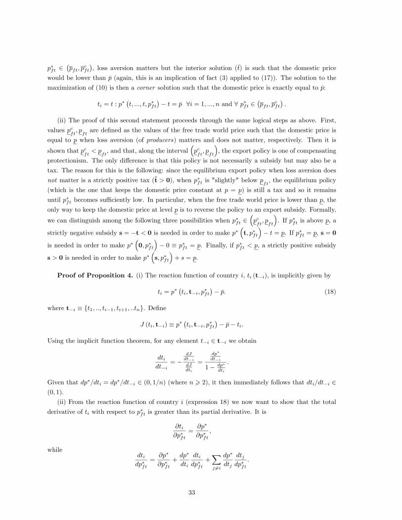
p∗ft ∈(pft, p
cft
), loss aversion matters but the interior solution (t) is such that the domestic price
would be lower than p (again, this is an implication of fact (3) applied to (17)). The solution to the
maximization of (10) is then a corner solution such that the domestic price is exactly equal to p:
ti = t : p∗(t, ..., t, p∗ft
)− t = p ∀i = 1, ..., n and ∀ p∗ft ∈
(pft, p
cft
).
(ii) The proof of this second statement proceeds through the same logical steps as above. First,
values pcft, pftare defined as the values of the free trade world price such that the domestic price is
equal to p when loss aversion (of producers) matters and does not matter, respectively. Then it is
shown that pcft< p
ft, and that, along the interval
(pcft, pft
), the export policy is one of compensating
protectionism. The only difference is that this policy is not necessarily a subsidy but may also be a
tax. The reason for this is the following: since the equilibrium export policy when loss aversion does
not matter is a strictly positive tax (t > 0), when p∗ft is "slightly" below pft, the equilibrium policy
(which is the one that keeps the domestic price constant at p = p) is still a tax and so it remains
until p∗ft becomes suffi ciently low. In particular, when the free trade world price is lower than p, the
only way to keep the domestic price at level p is to reverse the policy to an export subsidy. Formally,
we can distinguish among the following three possibilities when p∗ft ∈(pcft, pft
). If p∗ft is above p, a
strictly negative subsidy s = −t < 0 is needed in order to make p∗(t, p∗ft
)− t = p. If p∗ft = p, s = 0
is needed in order to make p∗(0, p∗ft
)− 0 ≡ p∗ft = p. Finally, if p∗ft < p, a strictly positive subsidy
s > 0 is needed in order to make p∗(s, p∗ft
)+ s = p.
Proof of Proposition 4. (i) The reaction function of country i, ti (t−i), is implicitly given by
ti = p∗(ti, t−i, p
∗ft
)− p. (18)
where t−i ≡ t1, .., ti−1, ti+1, ..tn. Define
J (ti, t−i) ≡ p∗(ti, t−i, p
∗ft
)− p− ti.
Using the implicit function theorem, for any element t−i ∈ t−i we obtain
dtidt−i
= −dJdt−idJdti
=
dp∗
dt−i
1− dp∗
dti
.
Given that dp∗/dti = dp∗/dt−i ∈ (0, 1/n) (where n > 2), it then immediately follows that dti/dt−i ∈(0, 1).
(ii) From the reaction function of country i (expression 18) we now want to show that the total
derivative of ti with respect to p∗ft is greater than its partial derivative. It is
∂ti∂p∗ft
=∂p∗
∂p∗ft,
whiledtidp∗ft
=∂p∗
∂p∗ft+dp∗
dti
dtidp∗ft
+∑j 6=i
dp∗
dtj
dtjdp∗ft
.
33
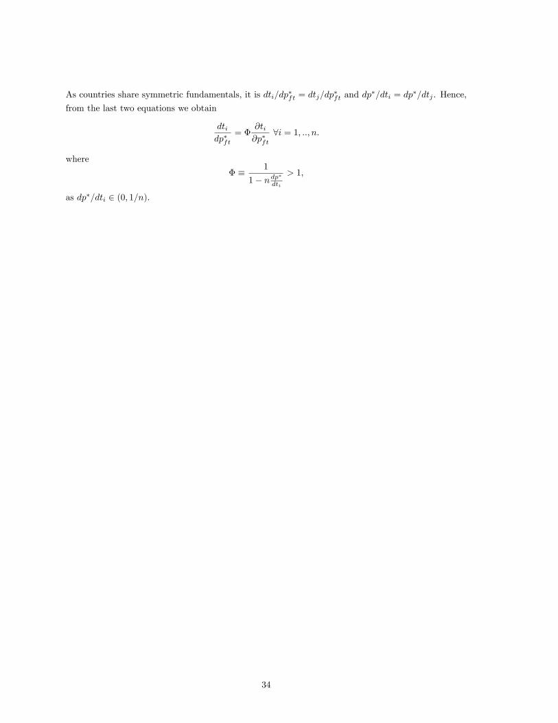
As countries share symmetric fundamentals, it is dti/dp∗ft = dtj/dp∗ft and dp
∗/dti = dp∗/dtj . Hence,
from the last two equations we obtain
dtidp∗ft
= Φ∂ti∂p∗ft
∀i = 1, .., n.
where
Φ ≡ 1
1− ndp∗dti> 1,
as dp∗/dti ∈ (0, 1/n).
34
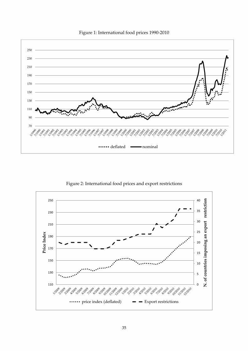
35
Figure 1: International food prices 1990‐2010
Figure 2: International food prices and export restrictions
70
90
110
130
150
170
190
210
230
250
deflated nominal
0
5
10
15
20
25
30
35
40
110
130
150
170
190
210
230
250
N. of countries imposing an export restriction
Price Index
price index (deflated) Export restrictions
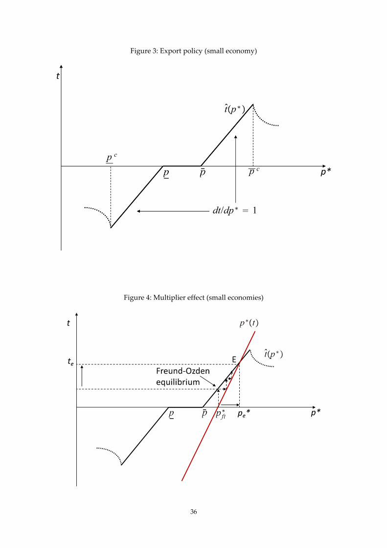
36
Figure 3: Export policy (small economy)
Figure 4: Multiplier effect (small economies)
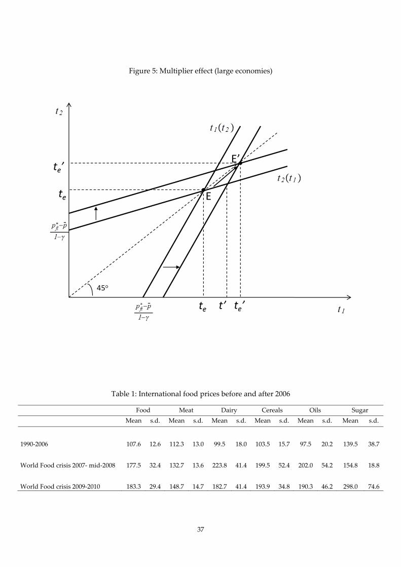
37
Figure 5: Multiplier effect (large economies)
Table 1: International food prices before and after 2006
Food Meat Dairy Cereals Oils Sugar
Mean s.d. Mean s.d. Mean s.d. Mean s.d. Mean s.d. Mean s.d.
1990‐2006 107.6 12.6 112.3 13.0 99.5 18.0 103.5 15.7 97.5 20.2 139.5 38.7
World Food crisis 2007‐ mid‐2008 177.5 32.4 132.7 13.6 223.8 41.4 199.5 52.4 202.0 54.2 154.8 18.8
World Food crisis 2009‐2010 183.3 29.4 148.7 14.7 182.7 41.4 193.9 34.8 190.3 46.2 298.0 74.6
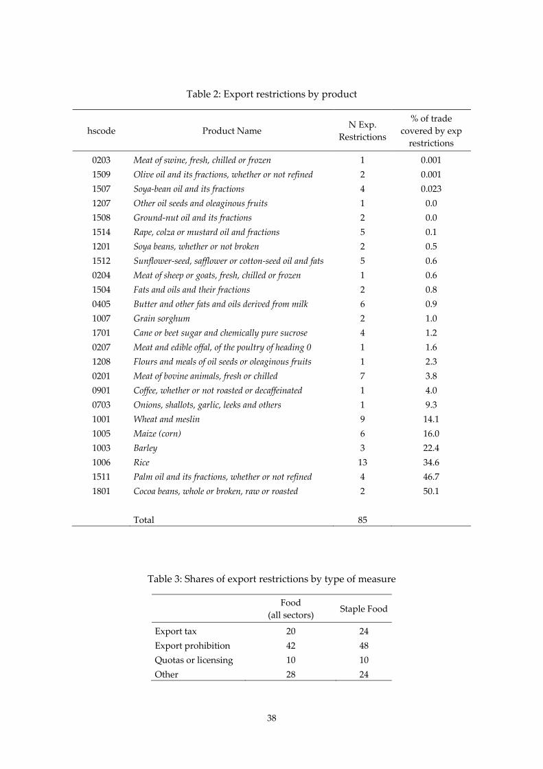
38
Table 2: Export restrictions by product
hscode Product Name N Exp.
Restrictions
% of trade
covered by exp
restrictions
0203 Meat of swine, fresh, chilled or frozen 1 0.001
1509 Olive oil and its fractions, whether or not refined 2 0.001
1507 Soya‐bean oil and its fractions 4 0.023
1207 Other oil seeds and oleaginous fruits 1 0.0
1508 Ground‐nut oil and its fractions 2 0.0
1514 Rape, colza or mustard oil and fractions 5 0.1
1201 Soya beans, whether or not broken 2 0.5
1512 Sunflower‐seed, safflower or cotton‐seed oil and fats 5 0.6
0204 Meat of sheep or goats, fresh, chilled or frozen 1 0.6
1504 Fats and oils and their fractions 2 0.8
0405 Butter and other fats and oils derived from milk 6 0.9
1007 Grain sorghum 2 1.0
1701 Cane or beet sugar and chemically pure sucrose 4 1.2
0207 Meat and edible offal, of the poultry of heading 0 1 1.6
1208 Flours and meals of oil seeds or oleaginous fruits 1 2.3
0201 Meat of bovine animals, fresh or chilled 7 3.8
0901 Coffee, whether or not roasted or decaffeinated 1 4.0
0703 Onions, shallots, garlic, leeks and others 1 9.3
1001 Wheat and meslin 9 14.1
1005 Maize (corn) 6 16.0
1003 Barley 3 22.4
1006 Rice 13 34.6
1511 Palm oil and its fractions, whether or not refined 4 46.7
1801 Cocoa beans, whole or broken, raw or roasted 2 50.1
Total 85
Table 3: Shares of export restrictions by type of measure
Food
(all sectors) Staple Food
Export tax 20 24
Export prohibition 42 48
Quotas or licensing 10 10
Other 28 24
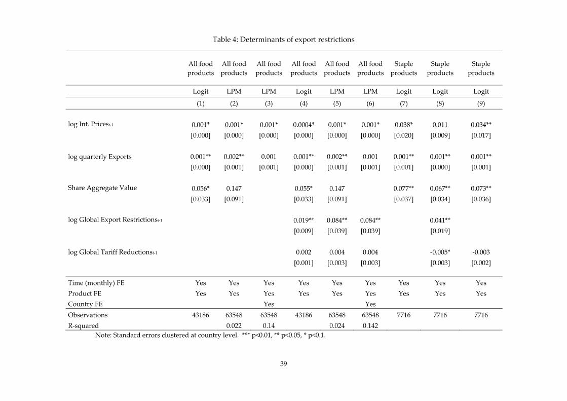
39
Table 4: Determinants of export restrictions
All food
products
All food
products
All food
products
All food
products
All food
products
All food
products
Staple
products
Staple
products
Staple
products
Logit LPM LPM Logit LPM LPM Logit Logit Logit
(1) (2) (3) (4) (5) (6) (7) (8) (9)
log Int. Pricest‐1 0.001* 0.001* 0.001* 0.0004* 0.001* 0.001* 0.038* 0.011 0.034**
[0.000] [0.000] [0.000] [0.000] [0.000] [0.000] [0.020] [0.009] [0.017]
log quarterly Exports 0.001** 0.002** 0.001 0.001** 0.002** 0.001 0.001** 0.001** 0.001**
[0.000] [0.001] [0.001] [0.000] [0.001] [0.001] [0.001] [0.000] [0.001]
Share Aggregate Value 0.056* 0.147 0.055* 0.147 0.077** 0.067** 0.073**
[0.033] [0.091] [0.033] [0.091] [0.037] [0.034] [0.036]
log Global Export Restrictionst‐1 0.019** 0.084** 0.084** 0.041**
[0.009] [0.039] [0.039] [0.019]
log Global Tariff Reductionst‐1 0.002 0.004 0.004 ‐0.005* ‐0.003
[0.001] [0.003] [0.003] [0.003] [0.002]
Time (monthly) FE Yes Yes Yes Yes Yes Yes Yes Yes Yes
Product FE Yes Yes Yes Yes Yes Yes Yes Yes Yes
Country FE Yes Yes
Observations 43186 63548 63548 43186 63548 63548 7716 7716 7716
R‐squared 0.022 0.14 0.024 0.142
Note: Standard errors clustered at country level. *** p<0.01, ** p<0.05, * p<0.1.
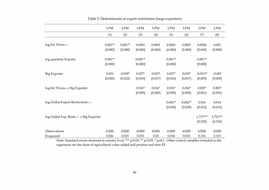
40
Table 5: Determinants of export restrictions (large exporters)
LPM LPM LPM LPM LPM LPM LPM LPM
(1) (2) (3) (4) (5) (6) (7) (8)
log Int. Prices t‐1 0.001** 0.001** 0.0001 0.0001 0.0001 0.0001 0.0004 0.001
[0.000] [0.000] [0.000] [0.000] [0.000] [0.000] [0.000] [0.000]
log quarterly Exports 0.001** 0.001** 0.001** 0.001**
[0.000] [0.000] [0.000] [0.000]
Big Exporter 0.033 0.039* 0.027* 0.033* 0.027* 0.033* ‐0.011** ‐0.007
[0.020] [0.022] [0.016] [0.017] [0.016] [0.017] [0.005] [0.005]
log Int. Pricest‐1 x Big Exporter 0.016* 0.016* 0.016* 0.016* 0.003* 0.003*
[0.009] [0.009] [0.009] [0.009] [0.001] [0.001]
log Global Export Restrictions t‐1 0.082** 0.082** 0.014 0.014
[0.039] [0.039] [0.012] [0.011]
log Global Exp. Restr. t‐1 x Big Exporter 1.717*** 1.721***
[0.529] [0.530]
Observations 63280 63280 63280 63280 63280 63280 63280 63280
R‐squared 0.026 0.025 0.031 0.03 0.034 0.033 0.116 0.115
Note: Standard errors clustered at country level. *** p<0.01, ** p<0.05, * p<0.1. Other control variables included in the
regression are the share of agricultural value added and product and time FE.
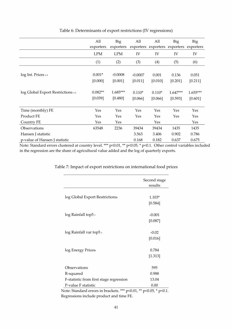
41
Table 6: Determinants of export restrictions (IV regressions)
All
exporters
Big
exporters
All
exporters
All
exporters
Big
exporters
Big
exporters
LPM LPM IV IV IV IV
(1) (2) (3) (4) (5) (6)
log Int. Prices t‐1 0.001* ‐0.0008 ‐0.0007 0.001 0.136 0.051
[0.000] [0.001] [0.011] [0.010] [0.201] [0.211]
log Global Export Restrictions t‐1 0.082** 1.685*** 0.110* 0.110* 1.647*** 1.655***
[0.039] [0.480] [0.066] [0.066] [0.593] [0.601]
Time (monthly) FE Yes Yes Yes Yes Yes Yes
Product FE Yes Yes Yes Yes Yes Yes
Country FE Yes Yes Yes Yes
Observations 63548 2236 39434 39434 1435 1435
Hansen J statistic 3.563 3.406 0.902 0.786
p‐value of Hansen J statistic 0.168 0.182 0.637 0.675
Note: Standard errors clustered at country level. *** p<0.01, ** p<0.05, * p<0.1. Other control variables included
in the regression are the share of agricultural value added and the log of quarterly exports.
Table 7: Impact of export restrictions on international food prices
Second stage
results
log Global Export Restrictionst 1.103*
[0.584]
log Rainfall top5 t ‐0.001
[0.087]
log Rainfall var top5 t ‐0.02
[0.016]
log Energy Pricest 0.784
[1.313]
Observations 595
R‐squared 0.988
F‐statistic from first stage regression 13.04
P‐value F statistic 0.00
Note: Standard errors in brackets. *** p<0.01, ** p<0.05, * p<0.1.
Regressions include product and time FE.
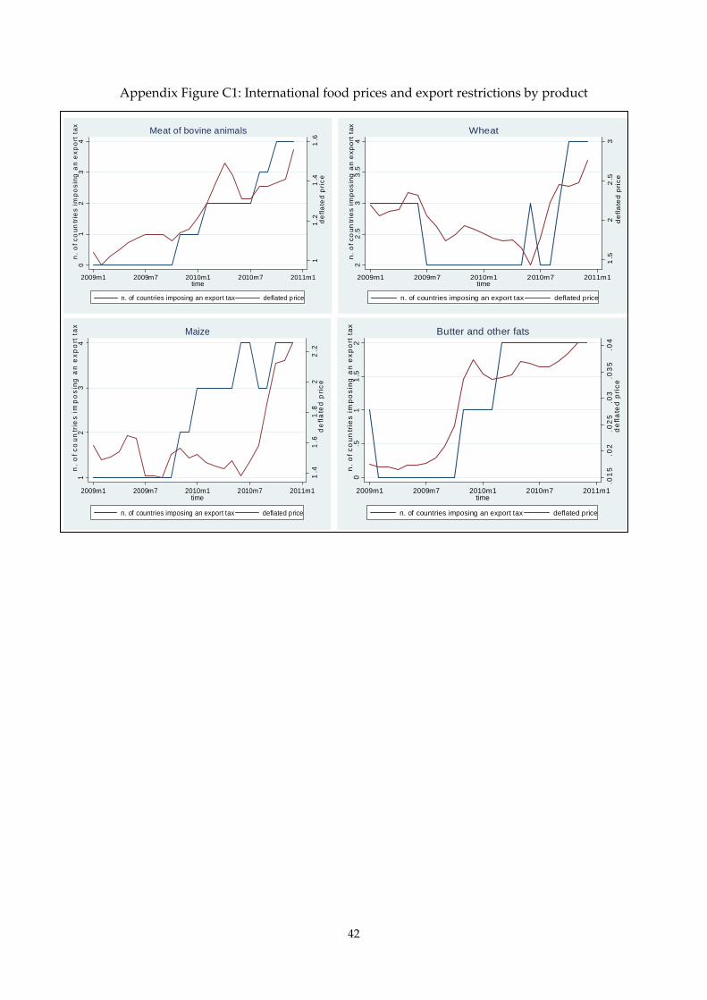
42
Appendix Figure C1: International food prices and export restrictions by product
11
.21
.41
.6d
efl
ate
d p
ric
e
01
23
4n
. o
f c
ou
ntr
ies
im
po
sin
g a
n e
xp
ort
ta
x
2009m1 2009m7 2010m1 2010m7 2011m1time
n. of countries imposing an export tax deflated price
Meat of bovine animals
1.5
22
.53
de
fla
ted
pri
ce
22
.53
3.5
4n
. o
f c
ou
ntr
ies
im
po
sin
g a
n e
xp
ort
ta
x
2009m1 2009m7 2010m1 2010m7 2011m1time
n. of countries imposing an export tax deflated price
Wheat
1.4
1.6
1.8
22
.2d
efl
ate
d p
ric
e
12
34
n.
of
co
un
trie
s i
mp
os
ing
an
ex
po
rt t
ax
2009m1 2009m7 2010m1 2010m7 2011m1time
n. of countries imposing an export tax deflated price
Maize
.01
5.0
2.0
25
.03
.03
5.0
4d
efl
ate
d p
ric
e
0.5
11
.52
n.
of
co
un
trie
s i
mp
os
ing
an
ex
po
rt t
ax
2009m1 2009m7 2010m1 2010m7 2011m1time
n. of countries imposing an export tax deflated price
Butter and other fats
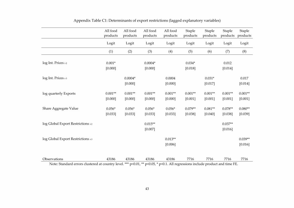
43
Appendix Table C1: Determinants of export restrictions (lagged explanatory variables)
All food
products
All food
products
All food
products
All food
products
Staple
products
Staple
products
Staple
products
Staple
products
Logit Logit Logit Logit Logit Logit Logit Logit
(1) (2) (3) (4) (5) (6) (7) (8)
log Int. Prices t‐2 0.001* 0.0004* 0.034* 0.012
[0.000] [0.000] [0.018] [0.014]
log Int. Prices t‐3 0.0004* 0.0004 0.031* 0.017
[0.000] [0.000] [0.017] [0.014]
log quarterly Exports 0.001** 0.001** 0.001** 0.001** 0.001** 0.001** 0.001** 0.001**
[0.000] [0.000] [0.000] [0.000] [0.001] [0.001] [0.001] [0.001]
Share Aggregate Value 0.056* 0.056* 0.056* 0.056* 0.079** 0.081** 0.078** 0.080**
[0.033] [0.033] [0.033] [0.033] [0.038] [0.040] [0.038] [0.039]
log Global Export Restrictions t‐2 0.015** 0.037**
[0.007] [0.016]
log Global Export Restrictions t‐3 0.013** 0.039**
[0.006] [0.016]
Observations 43186 43186 43186 43186 7716 7716 7716 7716
Note: Standard errors clustered at country level. *** p<0.01, ** p<0.05, * p<0.1. All regressions include product and time FE.
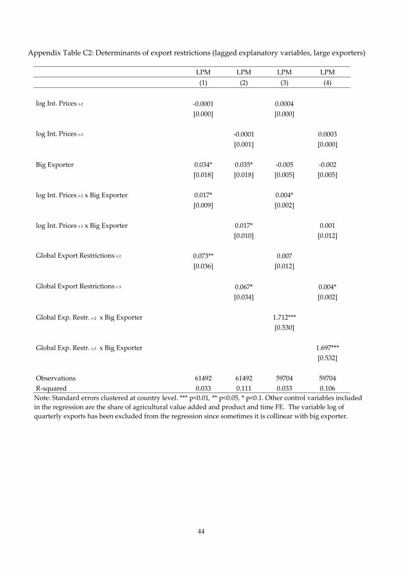
44
Appendix Table C2: Determinants of export restrictions (lagged explanatory variables, large exporters)
LPM LPM LPM LPM
(1) (2) (3) (4)
log Int. Prices t‐2 ‐0.0001 0.0004
[0.000] [0.000]
log Int. Prices t‐3 ‐0.0001 0.0003
[0.001] [0.000]
Big Exporter 0.034* 0.035* ‐0.005 ‐0.002
[0.018] [0.018] [0.005] [0.005]
log Int. Prices t‐2 x Big Exporter 0.017* 0.004*
[0.009] [0.002]
log Int. Prices t‐3 x Big Exporter 0.017* 0.001
[0.010] [0.012]
Global Export Restrictions t‐2 0.073** 0.007
[0.036] [0.012]
Global Export Restrictions t‐3 0.067* 0.004*
[0.034] [0.002]
Global Exp. Restr. t‐2 x Big Exporter 1.712***
[0.530]
Global Exp. Restr. t‐3 x Big Exporter 1.697***
[0.532]
Observations 61492 61492 59704 59704
R‐squared 0.033 0.111 0.033 0.106
Note: Standard errors clustered at country level. *** p<0.01, ** p<0.05, * p<0.1. Other control variables included
in the regression are the share of agricultural value added and product and time FE. The variable log of
quarterly exports has been excluded from the regression since sometimes it is collinear with big exporter.
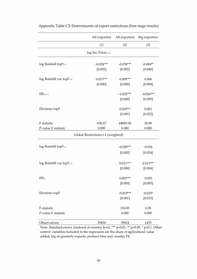
45
Appendix Table C3: Determinants of export restrictions (first stage results)
All exporters All exporters Big exporters
(1) (2) (3)
log Int. Prices t‐1
log Rainfall top5 t‐1 ‐0.024*** ‐0.059*** ‐0.084**
[0.002] [0.002] [0.040]
log Rainfall var top5 t‐1 0.013*** 0.009*** 0.006
[0.000] [0.000] [0.004]
ER‐k, t‐1 ‐0.032*** ‐0.036***
[0.000] [0.005]
Elections top5 0.019*** 0.003
[0.001] [0.022]
F statistic 638.27 44883.08 28.89
P‐value F statistic 0.000 0.000 0.000
Global Restrictions t‐1 (weighted)
log Rainfall top5 t‐1 ‐0.030*** ‐0.036
[0.002] [0.024]
log Rainfall var top5 t‐1 0.011*** 0.013***
[0.000] [0.004]
ER‐k 0.002*** ‐0.001
[0.000] [0.005]
Elections top5 ‐0.019*** ‐0.025*
[0.001] [0.013]
F statistic 310.85 6.98
P‐value F statistic 0.000 0.000
Observations 39434 39434 1435
Note: Standard errors clustered at country level. *** p<0.01, ** p<0.05, * p<0.1. Other
control variables included in the regression are the share of agricultural value
added, log of quarterly exports, product time and country FE.
Recommended