Foreign Institutional Investor Trading and Future Returns:
Evidence From an Emerging Economy
Murugappa (Murgie) Krishnan William Paterson University
Srinivasan Rangan Indian Institute of Management, Bangalore
First Version: June 10, 2015
This Version: February 11, 2016
This working paper is part of the NSE-NYU Stern School of Business Initiative for the Study of the
Indian Capital Markets. The authors acknowledge the support of the initiative. The views expressed in
this working paper are those of the authors and do not necessarily represent those of NSE or NYU. We
thank Vinod Ramachandran, Sivanand Jothy, and Sanjeev Kumar for their excellent research
assistance. We sincerely thank Nagapurnand Prabhala (discussant), Venky Panchapagesan, and
seminar participants at the 2015 NSE-NYU conference and at the Indian Institute of Technology,
Chennai for their comments and suggestions. This version of the paper supersedes an earlier version
of this paper that largely examined FII behavior around earnings announcements.

Foreign Institutional Investor Trading and Future Returns: Evidence
From an Emerging Economy
Abstract: This study presents evidence that Foreign Institutional Investor (FII) trades are
negatively related to future stock returns. For our sample period, portfolios of stocks that are
formed based on positive, zero, and negative FII quarterly net buying yield average quarterly
returns of 1.6%, 3.8%, and 2.4%, respectively. This suggests that investing in stocks in which
FIIs do not trade yields superior returns to those in which they trade. Further, their sells
perform better than their buys. We employ panel regressions to document a significant
negative relation between FII trading and future 3-month and 12-month returns after
controlling for several firm characteristics. The poor performance is magnified when FIIs
trade in small stocks and when they trade more frequently than average. We also find that
their quarterly net buying is negatively associated with returns during subsequent earnings
announcement dates. Further, their trades during the announcements also generate poor
performance in the three-month post-announcement period.
Keywords: Foreign Institutional Investors, Institutional Trading, Earnings Announcements,
Investment Performance.

1
1. Introduction
Institutional investors who pick stocks spend substantial amounts acquiring and
processing information with the intention of generating trading profits. The economic
significance of these amounts has engendered a debate and led to several studies on whether
institutions are ‘smart money’ traders. While most of this research focuses on U.S.
institutions, a small group of academics have examined the question of whether institutions
that invest in foreign countries (FIIs) are successful at picking stocks.
Some argue that FIIs are endowed with superior expertise and resources by virtue of
being global firms, and are hence likely to be successful portfolio managers. For example,
according to IOSCO (2012), “FIIs are highly specialized and manage substantial capital, can
enhance market features in many ways, including increasing liquidity, influencing market
psychology, and improving disclosures and corporate governance.” Others contend that FIIs
are likely to be disadvantaged in terms of experience and access to information vis-à-vis the
incumbent domestic investors (Brennan and Cao (1997)) and hence likely to underperform.
Additionally, local governments tend to tightly regulate foreign investors in terms of the types
of securities that they can trade and thus limit their performance potential.
The evidence on the FII stock-level investment performance in multiple markets
(including Finland, Indonesia, Japan, South Korea, and Taiwan) is mixed. While Grinblatt
and Keloharju (2000), Huang and Shiu (2009), and Bae, Min, and Jung (2011) conclude that
FIIs generate superior performance, Kang and Stulz (1997), Dvorak (2005), and Choe, Kho,
and Stulz (2005) report the opposite. Be that as it may, our intention is not to resolve prior
mixed evidence, as this evidence relates to multiple countries with differences in trading
environments as well as information qualities and flows. Additionally, methodologies differ
widely across studies. Our research objective is to evaluate the investing skill of FIIs in India,

2
a large emerging market that is relatively unexplored.1 While there are many anecdotal
references in the Indian financial press of significant FII activity in Indian financial markets,
formal evidence of their role, and the consequences of their activity, is limited.
In India, an FII refers to an institution established or incorporated outside India which
proposes to make investments in securities in India. To be able to trade, FIIs have to be
registered with the Securities and Exchange Board of India (SEBI).2 The label “FII” masks
considerable heterogeneity. FIIs include overseas mutual funds and similar financial market
participants whom we may tend to regard a priori as professional and sophisticated. But it
also includes smaller players and only some FIIs may have the resources for rigorous
analysis before making an investment decision.
FII trades can be classified into two broad categories: trades on their own account
and trades on behalf of foreign investors. To facilitate the latter, FIIs issue derivative
instruments known as P-Notes, via investment banks. FIIs initiate trades on behalf of their
clients and then P-Notes are issued to the clients to indicate that shares are held by the FII on
behalf of the client. Information on the identity of P-Note holders is typically difficult to
establish, at least at the time of the trade. Thus, P-Notes offer foreign investors an
opportunity to get exposure to the Indian market without having to register as an FII with
SEBI.3 A frequent claim in the financial press is that P-Note holders are connected to Indian
corporate entities and thus help the latter to retain control in the investee firms or to even
avoid paying taxes in India (see for example, Economic Times (2014)). Thus, it is possible
1 In terms of economic significance, the National Stock Exchange (NSE) whose firms we study is the twelfth
largest exchange in terms of market capitalization at the beginning of 2015.
(https://en.wikipedia.org/wiki/List_of_stock_exchanges). Further, on cumulative foreign direct investment by
2013, India ranked seventh in Asia and twenty-sixth in the world
(https://en.wikipedia.org/wiki/List_of_countries_by_FDI_abroad). 2 The criteria to qualify for registration are contained in the SEBI (Foreign Institutional Investor) Regulations,
1995. In January 2014, SEBI issued the SEBI (Foreign Portfolio Investors) Regulations), 2014. This regulation
employs the term Foreign Portfolio Investors to define a broader class of foreign investors that consists of FIIs
and Qualified Foreign Investors. In this paper, we continue to use the label FII as most of the academic
literature still does so. 3 See Parikh (2014) for a more detailed discussion of the structure of the market for P-Notes.

3
that FII trades related to P-Notes are motivated by the desire to retain corporate control or
avoid taxes, potentially at the expense of a return maximization objective. Hence, whether
FIIs are successful portfolio managers, and whether they even care about market
performance, are open questions.
Our first test of evaluating FII investing skill is similar to that of Gompers and
Metrick (2001) and Yan and Zhang (2009) who study U.S. institutional investors. We
estimate panel regressions of three month and twelve month returns on lagged quarterly FII
net buying and several firm characteristics. The coefficient on the net buying variable is
indicative of FIIs’ informedness that is incremental to that obtained by just picking stocks
based on certain firm characteristics.
If FIIs possess private information about a future event / outcome, they can trade
ahead of that outcome (for example, knowledge of an order that the firm has received but yet
to announce to the public). In our second test of FII informedness, we use earnings
announcements as future outcomes and test if FII trading is in the same direction as one-
quarter ahead unexpected earnings and announcement returns.
Even without being privately informed, FIIs can simply time their trades to take
advantage of a known relation between public information and future returns. This would be a
lower threshold of investing skill. In this study, we test FIIs’ ability to trade to exploit the
post-earnings announcement drift (PEAD) anomaly (Bernard and Thomas (1989)).
Specifically, we correlate FII net trading during the earnings announcement with (a)
announced unexpected earnings and (b) post-announcement returns. Positive correlations
with both variables would be consistent with FIIs trading to take advantage of the PEAD.
Our study employs a database of daily stock-level trades of FIIs in India for the years
2003-2014. This firm-level data was not available till SEBI began releasing masked FII
transaction data in a step towards compliance with a promise made in reply to a parliamentary

4
question. We aggregate daily trades over a quarter to construct a measure of quarterly net
buying. Our first finding is that FIIs’ trades are on average unprofitable over the sample
period. Portfolios of stocks that are formed based on positive, zero, and negative FII quarterly
net buying yield average quarterly returns of 1.6%, 3.8%, and 2.4%, respectively. This
suggests that investing in stocks in which FIIs do not trade yields superior returns to those in
which they trade. Further, their sells perform better than their buys. Panel regressions of 3-
month and 12-month returns confirm that quarterly FII trading is negatively associated with
subsequent returns. A 10% increase in FII net buying is associated with 3% (6%) decline in
returns in the subsequent quarter (year).
To understand the causes of this poor performance, we separate the sample into (a)
small/large stocks and (b) stocks that are frequently traded by FIIs and those that are less
frequently traded. Fewer analysts follow small firms and these firms face more uncertainty
and are hence harder value. Hence, we expect that the relation between FII trading and
subsequent returns to be more negative for small firms. Our results, especially for one-year
returns, are consistent with this prediction. Researchers in behavioural finance have
developed theoretical models that posit that traders who are overconfident trade too much and
consequently suffer losses (Odean (1998); Barber and Odean (2000); Daniel and Hirshleifer
(2015)). Therefore, we predict the FII trading losses will be magnified when they trade more
frequently. We divide our sample based on the median number of transactions per quarter
(buys + sells) and find that more frequent FII trading magnifies the negative relation between
FII trading and subsequent returns. Thus, the poor performance of FIIs in India can be partly
attributed to excessive trading.
We also examine the relation between FII trading and subsequent earnings surprises
and announcement returns. We find that net quarterly FII buying is unrelated to unexpected
earnings for the next quarter. In contrast, net buying is significantly negatively related to

5
earnings announcement returns: a 10% increase in lagged net buying is associated with 0.7%
decrease in earnings announcement returns. The inability to predict earnings news and the
poor returns around earnings announcements strengthens the conclusion that FIIs in India do
not behave like informed traders. This contrasts with a bulk of the U.S. evidence that
institutional trades are positively associated with subsequent earnings news (Gompers and
Metrick (2001); Yan and Zhang (2009)).
Lastly, our examination of FII net buying during the earnings announcement suggests
that they do not exploit the post-earnings announcement drift. For our sample, buying firms in
the top quartile of unexpected earnings and shorting firms in the bottom quartile, generates
average market-adjusted returns of 6.5% over the next 3 months. In contrast, we find that FII
net buying during the earnings announcement is not related to unexpected earnings and is
negatively related to subsequent three-month stock returns. We conclude that FIIs fail to
exploit the PEAD strategy.
Our study adds to the evidence on FII performance by examining their medium-term
performance in a relatively unexplored economy, India. In a contemporaneous study of Indian
FIIs, Acharya, Anshuman, and Kumar (2014) find that abnormal returns associated with
unusually low (high) daily FII flow innovations reverse (do not reverse) over the next two
weeks, especially when global volatility is high. They interpret the low FII daily innovations
leading to price reversals as evidence of limits to arbitrage. Our evidence suggests that
reversals occur over longer periods – three months to one year, and are also concentrated
around earnings announcements. Further, we find that both FII buys and sells are associated
with poor subsequent performance. Our evidence that unusually high trading magnifies FII
trading losses complements work on trading losses associated with overconfident individuals
who trade too frequently (Barber and Odean (2000); Daniel and Hirshleifer (2015)).

6
The explanations for the underperformance of FIIs in India could be behavioural or
rational. FIIs could be poor at picking stocks or other investors could follow FIIs, even
though they are not smart and thus temporarily push prices away from fundamentals. Rational
explanations would include losses related to global portfolio diversification, tax avoidance
strategies, and the desire to maintain corporate control. Distinguishing between these
explanations would provide an interesting subject for future research.
The rest of the paper is organized as follows. In section 2, we provide a brief review
of prior literature that relates to our research. Section 3 describes our data sources and sample
selection process and section 4 presents the variable definitions and main empirical models.
In section 5, we present our results, and in section 6 we discuss our conclusions.
2. Prior Literature
We organize our brief overview of prior work on the informedness of institutional
investors into (a) U.S. based evidence and (b) evidence on FIIs.
2.1. U.S. Evidence
A sizable literature examines the profitability of trades by U.S. institutional investors
as a group. The conclusion from most studies in this literature is that institutional investors
are informed and profit from their trades; their net buying is positively associated with
subsequent stock returns. There are four key aspects to this conclusion. First, these findings
obtain when researchers examine the relation between changes in quarterly shareholdings and
subsequent medium-term returns of 3 months to one year (Nofsinger and Sias (1999);
Gompers and Metrick (2001); Bennet Sias, and Starks (2003); Sias (2004); Yan and Zhang
(2009)). Second, Pucket and Yan (2011) document that even intra-quarter trades are
profitable – the average difference in returns between institutional buys and sells from trade

7
execution date to the end of the quarter is positive. Third, several studies show that quarterly
change in institutional shareholdings is positively related to subsequent earnings surprises and
earnings announcement returns (Ali, Durtschi, Lev, and Trombley (2004); Ke and Petroni
(2004); Yan and Zhang (2009); Campbell, Ramadorai, and Schwartz (2009); Baker, Litov,
Wachter, and Wurgler (2010)). Fourth, a few studies that examine trades over relatively short
intervals just before earnings announcements document a positive relation between
institutional net buying and earnings announcement returns (Berkman and McKenzie (2012);
Hendershott, Livdan, and Schurhoff (2014)).
The finding that institutions behave like informed traders is not without exceptions.
Cai and Zheng (2004) find that quarterly institutional trading has negative predictive ability
for next quarter’s returns using a vector autoregression framework. Bushee and Goodman
(2007) find that neither institutions collectively nor any specific class of institutions, both
trade in the direction of future earnings surprises and cash out subsequent to these surprises.
Griffin, Shu and Topaloglu (2012) study the trading behavior of institutions that are clients of
investment banks and find that institutional net buying over two-, five-, ten-, and twenty-day
windows do not generate abnormal profits before earnings, takeover, and seasoned equity
offering announcements. More recently, Edelen, Ince, Kladlec (2015) find that institutional
investors fail to tilt their portfolios to take advantage of seven well-known anomalies:
profitability, corporate investment, earnings quality, financing, financial distress, momentum.
Instead, they trade contrary to anomaly prescriptions.
2.2 Evidence on FII trades
The research on FIIs’ trades also generates mixed evidence on informedness /
profitability. Evidence that FIIs are informed is provided in Grinblatt and Keloharju (2000),
Huang and Shiu (2009), and Bae, Min, and Jung (2011). Using daily data for the 16 largest

8
Finnish stocks, Grinblatt and Keloharju (2000) find that the daily trades of foreigners is
positively associated with returns over the subsequent 6 months. Huang and Shiu (2009) find
that, in Taiwan, stocks with high foreign ownership outperform stocks with low foreign
ownership. Bae, Min, and Jung (2011) find that for Korean stocks, foreign investors’ buys
significantly outperform their sells over the 12-month period following their trades.
The opposite evidence that FIIs are not informed is provided in Kang and Stulz
(1997), Dvorak (2005), and Choe, Kho, and Stulz (2005). Kang and Stulz (1997) find that
foreign investors in Japanese stocks underperform relative to the market portfolio in terms of
monthly returns, but this underperformance is not statistically significant. Using transaction-
level data on a sample of 30 Indonesian stocks, Dvorak (2005) finds that foreign investors
underperform relative to domestic investors. Choe, Kho, and Stulz (2005) using Korean
intraday price data, show that foreign money managers pay more than domestic money
managers when they buy and receive less when they sell for medium and large trades.
A few studies also examine FII trades around earnings announcements. Seasholes
(2003) finds that foreign investors in Taiwan and South Korea accumulate shares before
positive earnings news and sell shares before negative earnings news. Eom, Hahn, and Sohn
(2010) find that, in Korea, foreign investors’ pre-announcement trades predict earnings
surprises, and that their trades after earnings announcements appear to exploit PEAD. In
contrast, a subsequent study of Korean stocks, Park, Lee, and Song (2013) document that pre-
announcement trading by foreign institutions does not forecast abnormal returns in the week
following the earnings announcement.
3. Data Sources and Sample
We obtain data from three sources: the PROWESS database of the Centre for
Monitoring Indian Economy Private Limited (CMIE), the website of the National Stock
9
Exchange of India (NSE), and the website of the National Securities Depositories Limited
(NSDL). PROWESS provides daily returns, prices, shares outstanding, and volumes;
quarterly and annual financial statement data; and quarterly data on FII ownership. The NSE
website (http://www.nseindia.com) is our source for earnings announcement dates. The
NSDL website contains the FII trade dataset.4 We study NSE-listed stocks alone as they tend
to be more frequently traded than stocks listed on the Mumbai Stock Exchange (BSE), the
other major Indian Stock exchange.
The sample period begins in the first quarter of 2003 (the first quarter for which firm-
level FII trades are available) and ends in the second quarter of 2014. The initial sample
consists of 57,596 firm-quarters for 1,846 NSE listed firms that have data on quarterly FII
trading and contemporaneous quarterly stock returns. We exclude 10,926 firm-quarters that
do not have data to compute one or more of the regression control variables (defined in
section 4). An additional 156 observations are dropped because of missing data on quarterly
FII ownership. The remaining 46,514 observations constitute the sample for the tests in which
three- and twelve-month returns are regressed on lagged quarterly FII trading. In a second set
of tests, we examine earnings announcement returns and post-announcement returns. For
these tests, the requirement that earnings announcement dates, unexpected earnings, and post-
announcement returns be available leaves us with a smaller sample of 28,460 firm-quarters.
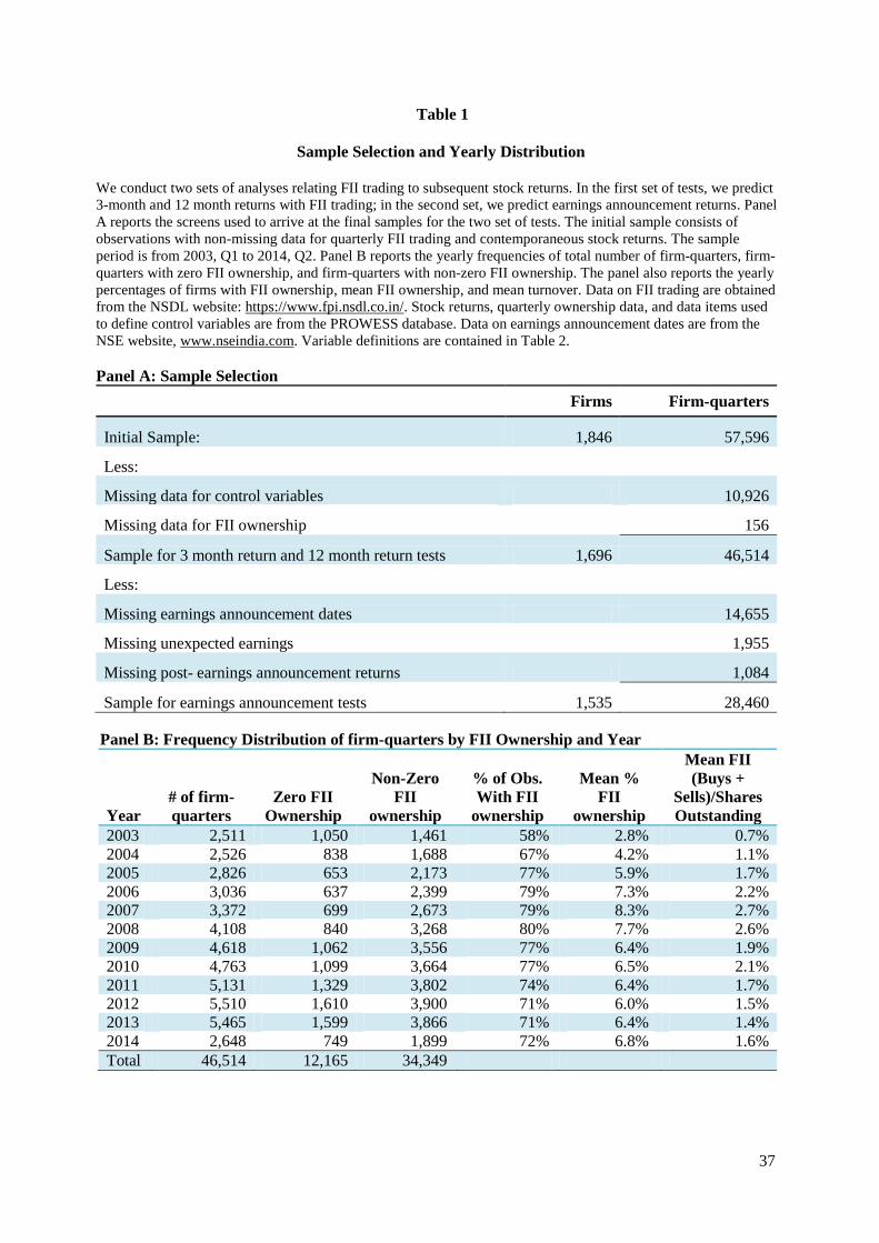
Panel A of Table 1 reports the screens employed to arrive at our final samples for the two sets
of tests.
Panel B of Table 1 presents the year-by-year distribution of the number of firm-
quarters with and without FII ownership. The percentage of firm-quarters with FII ownership
increases from 58% in 2003 to 80% in 2008, the year when the recent financial crisis peaked.
4 This data is freely available at
https://www.fpi.nsdl.co.in/web/StaticReports/FIITradeWise2008/FIITradeWise2008.htm. We thank Shyam
Benegal who was instrumental in causing the data to become available in the public domain.
10
Subsequently, the percentage steadily drops to 72% in 2014 suggesting that the crisis had a
significant impact on FII participation in India. Panel B reports a similar trend for mean
percentage FII ownership. After peaking at 7.7% in 2008, that mean drops to 6.8% in 2014.
The last column of Panel B reports a measure of mean FII turnover. We compute this measure
for each firm-quarter by adding the aggregate shares bought and sold by FIIs in that quarter
and dividing this sum by beginning of period shares outstanding. Interestingly, mean FII
turnover increases until 2008 when it reaches 2.6% and then drops down to 1.4% by 2014. In
general, FIIs have been trading less after the 2008 crisis.
4. Variables and Models
In this section, we define the dependent variables (stock returns), main independent
variables (lagged FII trading), and regression control variables. We then present the models
that evaluate the profitability of FII trading, where we forecast stock returns with lagged FII
trading.
4.1. Stock returns
Our first two dependent variables are three-month and twelve-month stock returns. To
measure them, we begin by defining the continuously compounded return on day t as the
logarithm of the ratio of the closing price on day t to the closing price on day t-1. Daily
closing prices reflect dividends and adjustments for stock splits. LEADRET3 (LEADRET12)
is defined as the sum of daily continuously compounded returns over three (twelve months).
Our second two dependent variables are earnings announcement returns and post-
announcement returns. We label the date on which firms announce quarterly financial results
as day 0. Earnings announcement return (ERET) is defined as the sum of continuously
compounded returns over the three-day interval (-1, +1). Post-announcement returns
11
(POSTERET) are computed over the three month interval (+2, +64), assuming 21 trading
days in a month. If a daily return is missing in a cumulation period, it is set to equal zero;
however, if daily returns are missing for two-thirds or more of any cumulation period, we
drop that observation. Our treatment of missing returns is similar to that of Hung, Li, and
Wang (2014).
4.2 FII Trading Measures
Our main independent variable is quarterly firm-level FII net buying. However, we
also examine quarterly buying and selling separately as FII buy and sell decisions might
differ in their ability to predict subsequent returns. When forecasting post-announcement
returns, FII net buying during the earnings announcement is the main independent variable
because we wish to evaluate if FIIs are able to profit from the PEAD anomaly.
The NSDL’ FII database’s basic unit of observation is trading activity by an FII for a
stock on a trading day on a specified exchange. The database reports six measures of trading
activity for each FII-stock-exchange-day quadruple: (a) the number of buys; (b) the number
of sells; (c) aggregate shares bought on a day; (d) aggregate shares sold on a day; (e) value of
shares bought; and (f) value of shares sold. Unfortunately, SEBI masks the FII identifying
codes and changes them every month; this renders FII-level analysis difficult. Therefore, for
each stock-trading day pair, we aggregate daily data across FIIs. Because we have no reason
to expect exchange-related effects, we also aggregate daily trades across exchanges (primarily
the BSE and the NSE). Thus, the basic unit of analysis of FII trading is a firm-date
observation.
To compute quarterly net FII buying, we begin by defining FII net trading for firm i
and day t (NETFII) as the difference between shares bought (BUYit) and shares sold
(SOLDit). We aggregate NETFII over a calendar quarter to obtain Q_NETBUY. We also

12
compute the sum of all FII buys (sells) in a quarter, Q_BUY (Q_SELL). For the earnings
announcement tests, we compute EA_NETBUY as the sum of net FII buying over days (-1,
+1). To control for cross-sectional differences in firm size, cumulated trading measures are
divided by shares outstanding at the beginning of the period over which trades are cumulated.
Lo and Wang (2000: 258) characterize this share turnover-type measure as “a natural measure
of trading activity.”
4.3. Control Variables
We rely on two prior studies of U.S. institutional trading - Gompers and Metrick
(2001) and Yan and Zhang (2009), to define firm characteristics that are likely to be
correlated with both FII trading and future returns. Before defining these variables, we
motivate their choice.
First, a large body of work on return predictability has established that small stocks,
high book-to-market stocks, and stocks with high recent returns have predictable future
returns. This predictability has been interpreted either as anomalous evidence that contradicts
market efficiency or as returns to stocks with higher risk. FII trades are likely to be correlated
with these characteristics either because FIIs wish to exploit anomalies or because of their
risk preferences. Second, because FIIs trade on behalf of their clients, they are governed by
fiduciary (prudence) considerations in their investment choices (Del Guercio (1996)).
Gompers and Metrick (2001) employ four firm characteristics that capture this fiduciary
motive: age, dividend yield, membership in the S&P 500, and return volatility. They predict
that institutional ownership will be positively related to age, dividend yield, and S&P 500
membership, and negatively related to volatility. Lastly, because institutions are likely to
demand liquid stocks, Gompers and Metrick (2001) suggest three indicators of liquidity that

13
are expected to be positively related to institutional trading: market capitalization, per-share
stock price, and share turnover.
Building on the above, with the exception of the S&P 500 dummy that is not relevant
to the Indian market, we include the following nine variables in the regressions of stock
returns on lagged FII trading:
1. MCAP: Market Capitalization at the beginning of the quarter in which FII trading is
measured.
2. BM: Book value of equity divided by MCAP. Book value of equity is measured either
on the date MCAP is measured or on the year end date of the most recently concluded
fiscal year.
3. LAGRET3: The cumulative return over the 3 months prior to the quarter over which
FII trading is measured.
4. LAGRET9: The cumulative return measured over the 9 months prior to the 3-month
period over which LAGRET3 is measured.
5. AGE: The number of years since the year of incorporation.
6. DIVY: Annual cash dividend paid in the fiscal year for which book value of equity is
measured, divided by MCAP.
7. VOL: The standard deviation of monthly returns over the twelve months before the
quarter in which FII trading is measured.
8. PRC: Share price at the beginning of the quarter.
9. TO: The average monthly volume divided by shares outstanding over the three
months before the quarter in which FII trading is measured.
If non-institutional investors follow institutions, an increase (decrease) in institutional
ownership of a stock could increase (decrease) the demand in that stock and thus influence
subsequent returns. Therefore, Gompers and Metrick (2001) argue that to evaluate the

14
investing skill of institutions, it is important to control for the level of institutional ownership
which reflect “demand shocks” for stocks held by institutions. Accordingly, we also include
the end-of-quarter FII ownership percentage (FIIP) when forecasting stock returns.
4.4. Regression Models
We evaluate FII trade profitability in three ways. First, we examine the relation
between quarterly FII trading and subsequent 3-month and 12-month returns. Second, we
predict earnings announcement returns with lagged quarterly FII trading. Third, we evaluate
the ability of FII trades during earnings announcements to forecast subsequent three-month
returns; this allows us to test if FIIs exploit the PEAD anomaly.
The first model that we estimate is:
where LEADRET3 and LEADRET12 are the one-quarter ahead and one-year ahead returns,
respectively, and Q_NETBUY is lagged quarterly FII net buying. The coefficient on
Q_NETBUY captures returns to the investing skill of FIIs (or lack thereof) that are
incremental to the returns obtained by just picking stocks based on the nine firm
characteristics (control variables). To account for unobserved firm heterogeneity and
economy-level factors that cause returns to vary, we include firm and quarter fixed effects in
all regressions. Standard errors are adjusted to account for heteroscedasticity and two-way
clustering, across firms and over quarters.
In our second model, we predict earnings announcement returns with quarterly FII net
buying in the quarter that just precedes the earnings announcement:

15
where ERET is the earnings-announcement return. Compared to Eq. (1), we include three
additional variables to explain earnings announcement returns: FII net buying during the
announcement (EA_NETBUY), unexpected earnings (UE), and market returns during the
announcement (MRET). Including EA_NETBUY allows us to measure the market reaction to
FII trades during the announcement. UE measures earnings news during the announcement
and is defined as the difference between EPS in quarter t and its lagged value, from four
quarters before, divided by the closing price per share measured on day -2 relative to the
earnings announcement. MRET is defined as the return on the CNX Nifty Index summed
over days -1 to +1. The index daily return is calculated as the daily percentage change in the
Index.
Our third model is intended to assess FIIs’ ability to forecast post-earnings
announcement returns. We focus here on their trading during the earnings announcements
(EA_NETBUY). The model we estimate is:
where POSTERET is the three-month post-announcement return. As with Eq. (2), we include
UE as an additional explanatory variable. But here it does not capture contemporaneous
earnings news; rather, it is included to confirm that the PEAD anomaly obtains in the Indian
market.
5. Results
16
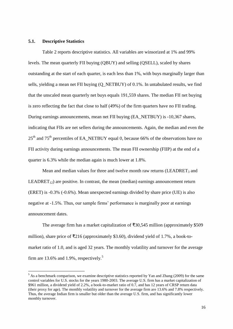
5.1. Descriptive Statistics
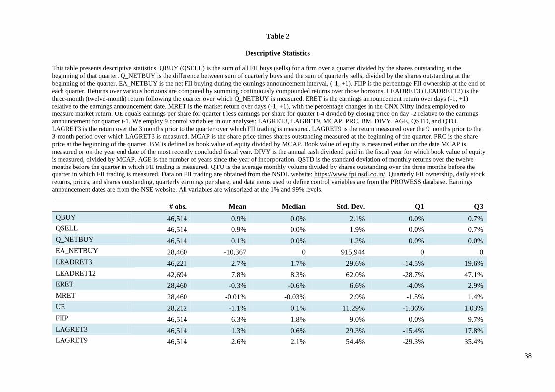
Table 2 reports descriptive statistics. All variables are winsorized at 1% and 99%
levels. The mean quarterly FII buying (QBUY) and selling (QSELL), scaled by shares
outstanding at the start of each quarter, is each less than 1%, with buys marginally larger than
sells, yielding a mean net FII buying (Q_NETBUY) of 0.1%. In untabulated results, we find
that the unscaled mean quarterly net buys equals 191,559 shares. The median FII net buying
is zero reflecting the fact that close to half (49%) of the firm quarters have no FII trading.
During earnings announcements, mean net FII buying (EA_NETBUY) is -10,367 shares,
indicating that FIIs are net sellers during the announcements. Again, the median and even the
25th
and 75th
percentiles of EA_NETBUY equal 0, because 66% of the observations have no
FII activity during earnings announcements. The mean FII ownership (FIIP) at the end of a
quarter is 6.3% while the median again is much lower at 1.8%.
Mean and median values for three and twelve month raw returns (LEADRET3 and
LEADRET12) are positive. In contrast, the mean (median) earnings announcement return
(ERET) is -0.3% (-0.6%). Mean unexpected earnings divided by share price (UE) is also
negative at -1.5%. Thus, our sample firms’ performance is marginally poor at earnings
announcement dates.
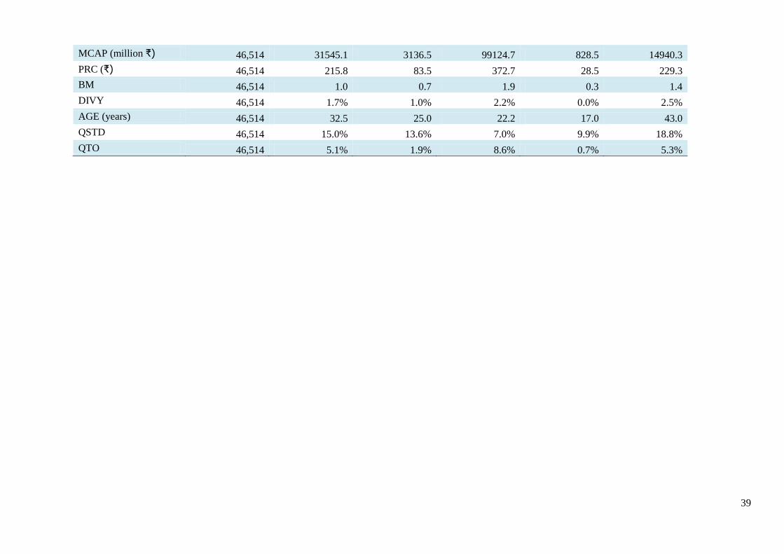
The average firm has a market capitalization of ₹30,545 million (approximately $509
million), share price of ₹216 (approximately $3.60), dividend yield of 1.7%, a book-to-
market ratio of 1.0, and is aged 32 years. The monthly volatility and turnover for the average
firm are 13.6% and 1.9%, respectively.5
5 As a benchmark comparison, we examine descriptive statistics reported by Yan and Zhang (2009) for the same
control variables for U.S. stocks for the years 1980-2003. The average U.S. firm has a market capitalization of
$961 million, a dividend yield of 2.2%, a book-to-market ratio of 0.7, and has 12 years of CRSP return data
(their proxy for age). The monthly volatility and turnover for the average firm are 13.6% and 7.8% respectively.
Thus, the average Indian firm is smaller but older than the average U.S. firm, and has significantly lower
monthly turnover.
17
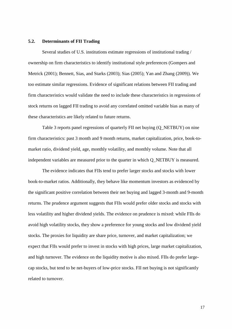
5.2. Determinants of FII Trading
Several studies of U.S. institutions estimate regressions of institutional trading /
ownership on firm characteristics to identify institutional style preferences (Gompers and
Metrick (2001); Bennett, Sias, and Starks (2003); Sias (2005); Yan and Zhang (2009)). We
too estimate similar regressions. Evidence of significant relations between FII trading and
firm characteristics would validate the need to include these characteristics in regressions of
stock returns on lagged FII trading to avoid any correlated omitted variable bias as many of
these characteristics are likely related to future returns.
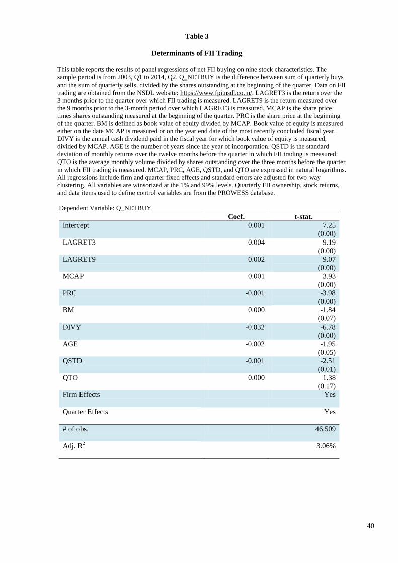
Table 3 reports panel regressions of quarterly FII net buying (Q_NETBUY) on nine
firm characteristics: past 3 month and 9 month returns, market capitalization, price, book-to-
market ratio, dividend yield, age, monthly volatility, and monthly volume. Note that all
independent variables are measured prior to the quarter in which Q_NETBUY is measured.
The evidence indicates that FIIs tend to prefer larger stocks and stocks with lower
book-to-market ratios. Additionally, they behave like momentum investors as evidenced by
the significant positive correlation between their net buying and lagged 3-month and 9-month
returns. The prudence argument suggests that FIIs would prefer older stocks and stocks with
less volatility and higher dividend yields. The evidence on prudence is mixed: while FIIs do
avoid high volatility stocks, they show a preference for young stocks and low dividend yield
stocks. The proxies for liquidity are share price, turnover, and market capitalization; we
expect that FIIs would prefer to invest in stocks with high prices, large market capitalization,
and high turnover. The evidence on the liquidity motive is also mixed. FIIs do prefer large-
cap stocks, but tend to be net-buyers of low-price stocks. FII net buying is not significantly
related to turnover.

18
While the evidence on market capitalization, past returns, and dividend yield is similar
to that for U.S. stocks, the evidence on trading preferences related to age, volatility, book-to-
market ratios, and share price differs. While not the focus of the paper, these differences raise
interesting questions about why institutional investor preferences could differ across countries
and exchanges.
5.3. Quarterly FII Trades and Subsequent 3 and 12 Month Returns
To provide a simple and intuitive answer to the question of whether FII trades are
profitable, we form portfolios based on the sign of net FII buying for a calendar quarter and
compute value-weighted portfolio returns over the next quarter. We evaluate three portfolios:
stocks where net FII buying is positive, negative, and zero, and label these the net buy, net
sell, and no trade portfolios. We repeat this exercise for each of the 46 quarters from the first
quarter of 2003 to the second quarter of 2014. We then calculate the product of 1 plus each
portfolio return over time to arrive at the future value of ₹1 at the end of the third quarter of
2014.
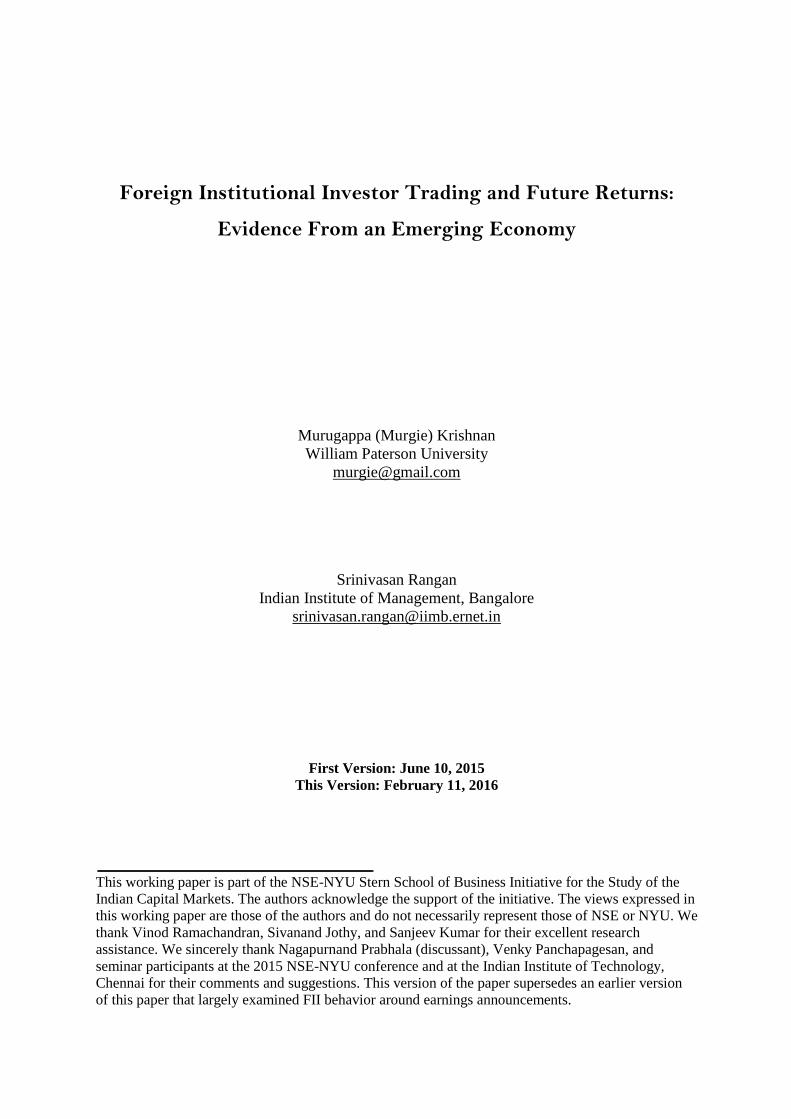
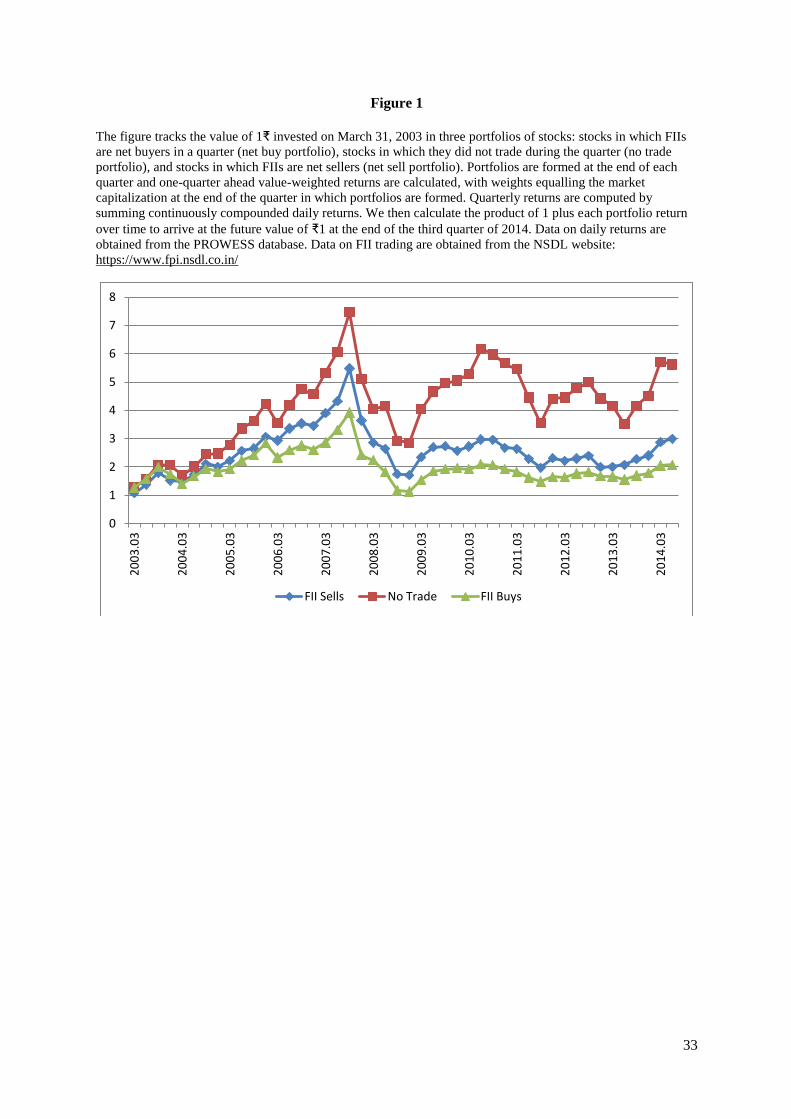
Figure 1 plots the value of investing ₹1 in each of the portfolios over time. All three
portfolios rise in value up to the third quarter of 2007, decline until the last quarter of 2008
(the period of the financial crisis) before displaying some cyclicality. If we had invested in
the net buy portfolio every quarter, ₹1 would have grown to ₹2.07 at the end of the third
quarter of 2014. A ₹1 investment in the net sell portfolio would be worth ₹2.99 after 46
quarters. The no-trade portfolio registers the highest returns of the three portfolios: ₹1
invested in a portfolio of stocks in which FIIs do not invest grows to ₹5.62. The implied
average quarterly returns for the net buy, no trade, and net sell portfolios are 1.6%, 3.8%, and
2.4%, respectively. Clearly, FII sells outperform FII buys. Moreover, interestingly, avoiding

19
stocks in which FIIs trade yields superior returns to strategies of following either FII buys or
sells.
The univariate analysis of Figure 1 tells us the FII sells outperform buys. Because FII
trading is associated with various firm characteristics, a portion of this return differential
could be attributed to these characteristics. The question that we are interested in is whether
FII net buying is incrementally associated with future returns after controlling for the returns
associated with the characteristics.
Table 4 reports panel regressions of 3-month and 12 month returns (LEADRET3 and
LEADRET12) on lagged quarterly FII net buying (Q_NETBUY) and control variables. The
regressions control for firm and quarter effects (not reported) and standard errors are adjusted
for clustering by firm and quarter. All regression variables are winsorized at the 1% and 99%
levels. We follow Gompers and Metrick (2001) and Yan and Zhang (2009) and express the
following strictly positive variables in natural logarithms: MCAP, PRC, AGE, QSTD, and
QTO.
When LEADRET3 is the dependent variable, the coefficient on Q_NETBUY is
negative and statistically significant confirming the univariate evidence in Figure 1. The
coefficient suggests that a 10% increase in FII net buying is associated with 3% decline in
returns in the subsequent quarter. In column (2), we replace FII net buying with separate
variables for FII buying and selling. The coefficients on both Q_BUY and Q_SELL are
statistically significant and negative and positive, respectively – stocks that FII buy
experience declines in returns in the next quarter and those that they sell experience return
increases. In columns (3) and (4), we report results when the dependent variable is the 12-
month return. Again, Q_NETBUY is statistically significant with a coefficient of -0.611 – a
10% increase in FII net buying is associated with 6% lower returns in the next one year.
Examining buying and selling separately in column (4) indicates that FII buys (sells) exhibit
20
negative (positive) twelve-month returns; the coefficient on Q_SELL, however, is not
statistically significant at the 10% level.
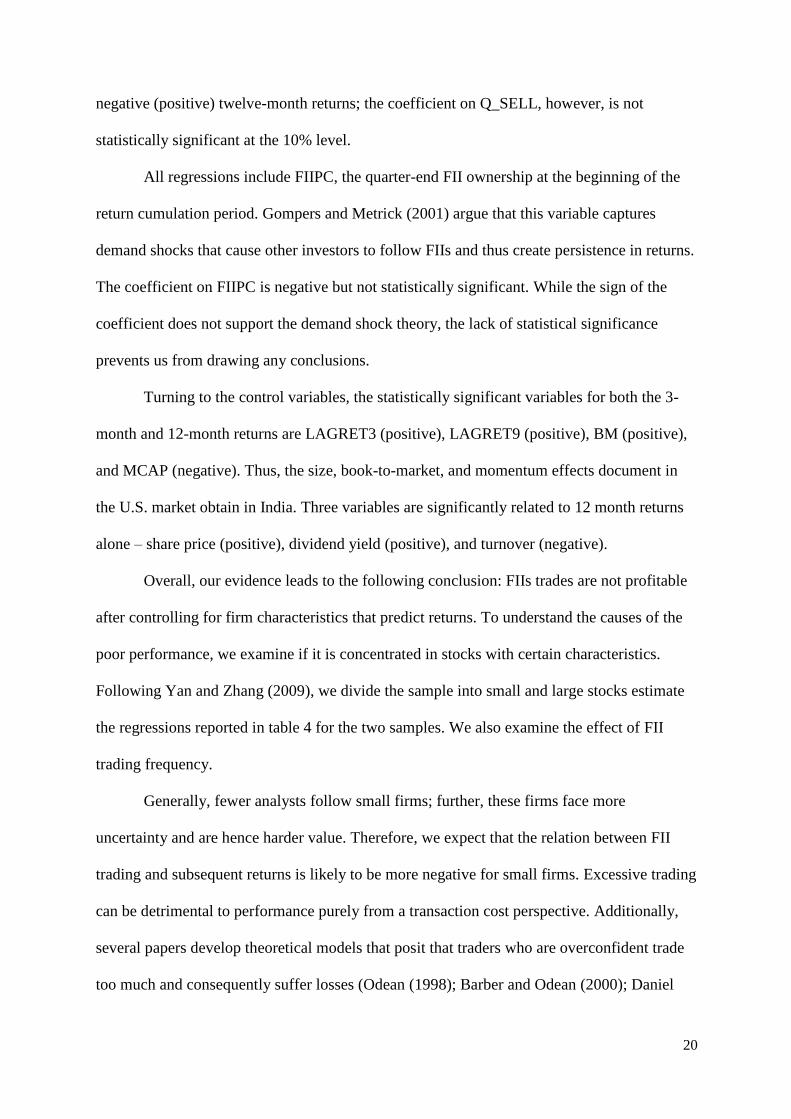
All regressions include FIIPC, the quarter-end FII ownership at the beginning of the
return cumulation period. Gompers and Metrick (2001) argue that this variable captures
demand shocks that cause other investors to follow FIIs and thus create persistence in returns.
The coefficient on FIIPC is negative but not statistically significant. While the sign of the
coefficient does not support the demand shock theory, the lack of statistical significance
prevents us from drawing any conclusions.
Turning to the control variables, the statistically significant variables for both the 3-
month and 12-month returns are LAGRET3 (positive), LAGRET9 (positive), BM (positive),
and MCAP (negative). Thus, the size, book-to-market, and momentum effects document in
the U.S. market obtain in India. Three variables are significantly related to 12 month returns
alone – share price (positive), dividend yield (positive), and turnover (negative).
Overall, our evidence leads to the following conclusion: FIIs trades are not profitable
after controlling for firm characteristics that predict returns. To understand the causes of the
poor performance, we examine if it is concentrated in stocks with certain characteristics.
Following Yan and Zhang (2009), we divide the sample into small and large stocks estimate
the regressions reported in table 4 for the two samples. We also examine the effect of FII
trading frequency.
Generally, fewer analysts follow small firms; further, these firms face more
uncertainty and are hence harder value. Therefore, we expect that the relation between FII
trading and subsequent returns is likely to be more negative for small firms. Excessive trading
can be detrimental to performance purely from a transaction cost perspective. Additionally,
several papers develop theoretical models that posit that traders who are overconfident trade
too much and consequently suffer losses (Odean (1998); Barber and Odean (2000); Daniel

21
and Hirshleifer (2015)). Overconfident investors tend to place excessive weight on their
private valuation and less on market valuation. This overconfidence leads to more frequent
trading and subsequent trading losses. In light of this evidence, we expect the relation
between FII trading and subsequent returns to be more negative for firms where FIIs trade
more frequently during the quarter.
We divide firms into two groups based on the median beginning of quarter market
capitalization. Large (small) stocks are defined as those with market capitalization greater
(less) than that of the median stock. Similarly, firms for which the number of FII transactions
exceeded (was less than) the median number of FII transactions (excluding no trades) were
classified as “frequently FII traded firms” (“less frequently FII traded firms”). The number of
transactions equals the sum of the number of buys and the number of sells in a quarter.
We re-estimate the regressions reported in Table 4 (Eq. (1)) for small/large stocks and
stocks where FIIs trade frequently/less frequently. Panel A of Table 5 reports the results for
small versus large stocks. For 3-month returns, the coefficient on Q_NETBUY is negative
and statistically significant for both small and large stocks. For small stocks, the coefficient
on Q_NETBUY is -0.392 which is 56% more negative than that for large stocks (-0.250). For
12-month returns, the coefficient on Q_NETBUY is -1.027 and statistically significant for
small stocks; for large stocks it is negative, but not statistically significant at the 10% level.
The collective evidence suggests that FII trades are less profitable when they trade in small
stocks.
Panel B of Table 5 reports the results for the frequently and less frequently FII-traded
stocks. For both three-month and one-year returns, the coefficient on Q_NETBUY is not
statistically significant for stocks where FII trade less frequently. In contrast, when FIIs trade
frequently, Q_NETBUY is negatively and significantly associated with subsequent returns.
For 3-month returns, the coefficient is -0.401 (t-statistic = -2.51); a 10% increase in FII

22
quarterly net buying is associate with 4% lower returns in the next quarter. Similarly, for one
year returns, a 10% increase in FII quarterly net buying is associated with 6.46% decrease
returns over the next one year. The lesson is: avoid (buy) stocks that FIIs buy (sell),
especially when their trading levels are relatively high.
5.4. FII Trades and Earnings Announcements
Our results thus far indicate that quarterly FII trading is negatively associated with
subsequent returns over intermediate horizons – three and twelve months. To provide more
direct evidence on FIIs’ investing skills, we examine the relation between FII trades and
future earnings news. We examine both unexpected earnings and earnings announcement
abnormal returns. Additionally, we also evaluate FII performance in the post-announcement
period.
Because large sample evidence on returns and volume around earnings
announcements for Indian firms is unavailable, we begin by providing descriptive evidence
on (a) market volume and FII trading around announcements and (b) return movements prior
to, during and subsequent to earnings announcements. In this manner, we confirm that return
and volume patterns documented in other countries are observed in India as well.
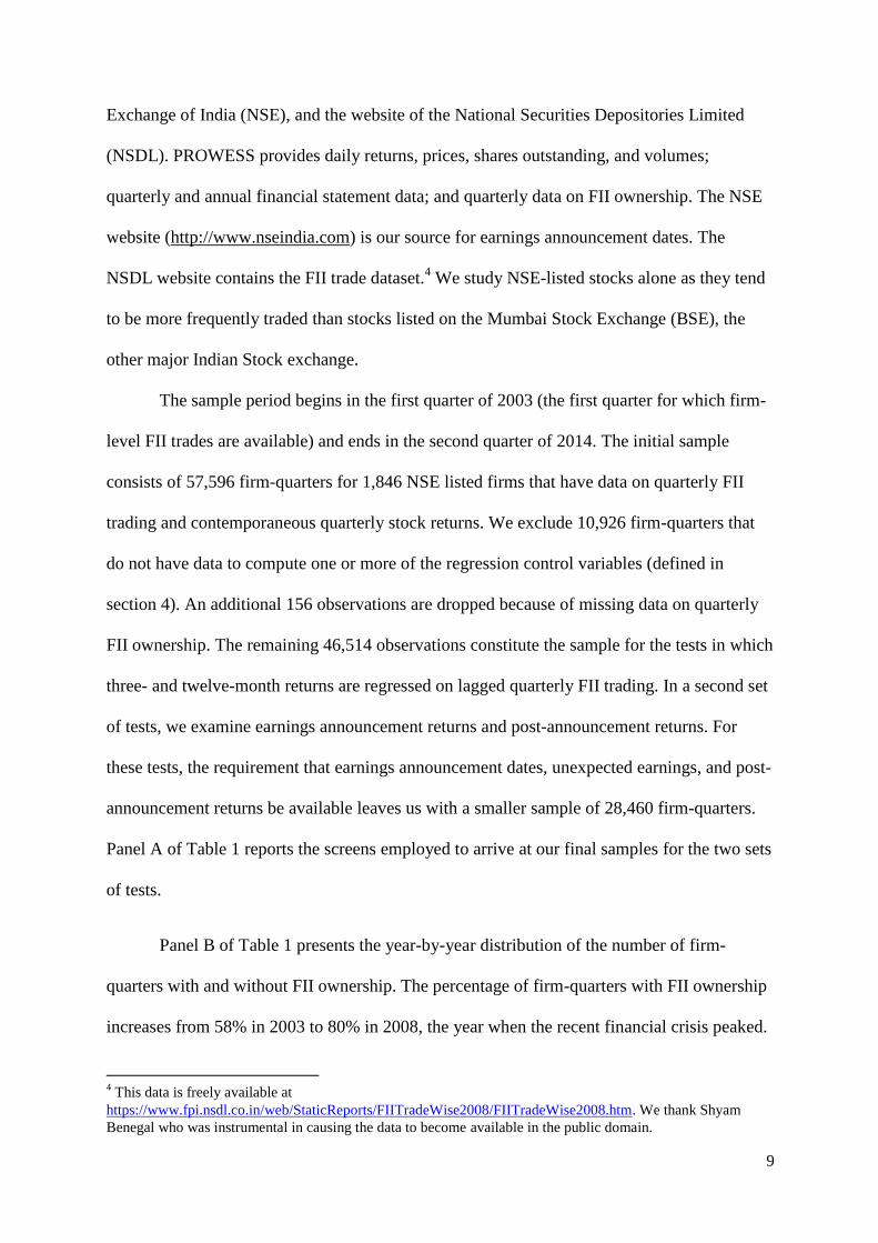
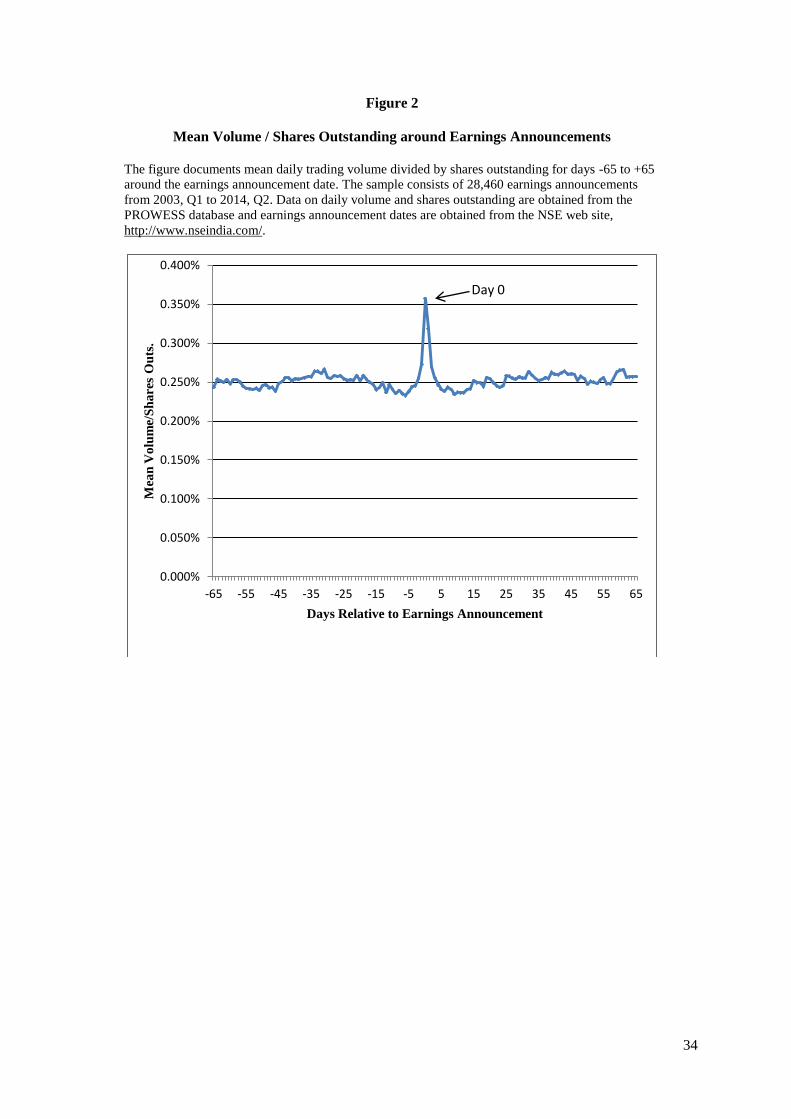
Figure 2 presents mean volume deflated by shares outstanding in the 130-day window
around the earnings announcement date. Average volume displays a significant spike on day
0. It hovers around 0.25% in the pre- and post-announcement periods, but touches 0.36% on
day 0 and 0.32% on day 1. We can safely conclude that earnings announcements stimulate
trading.
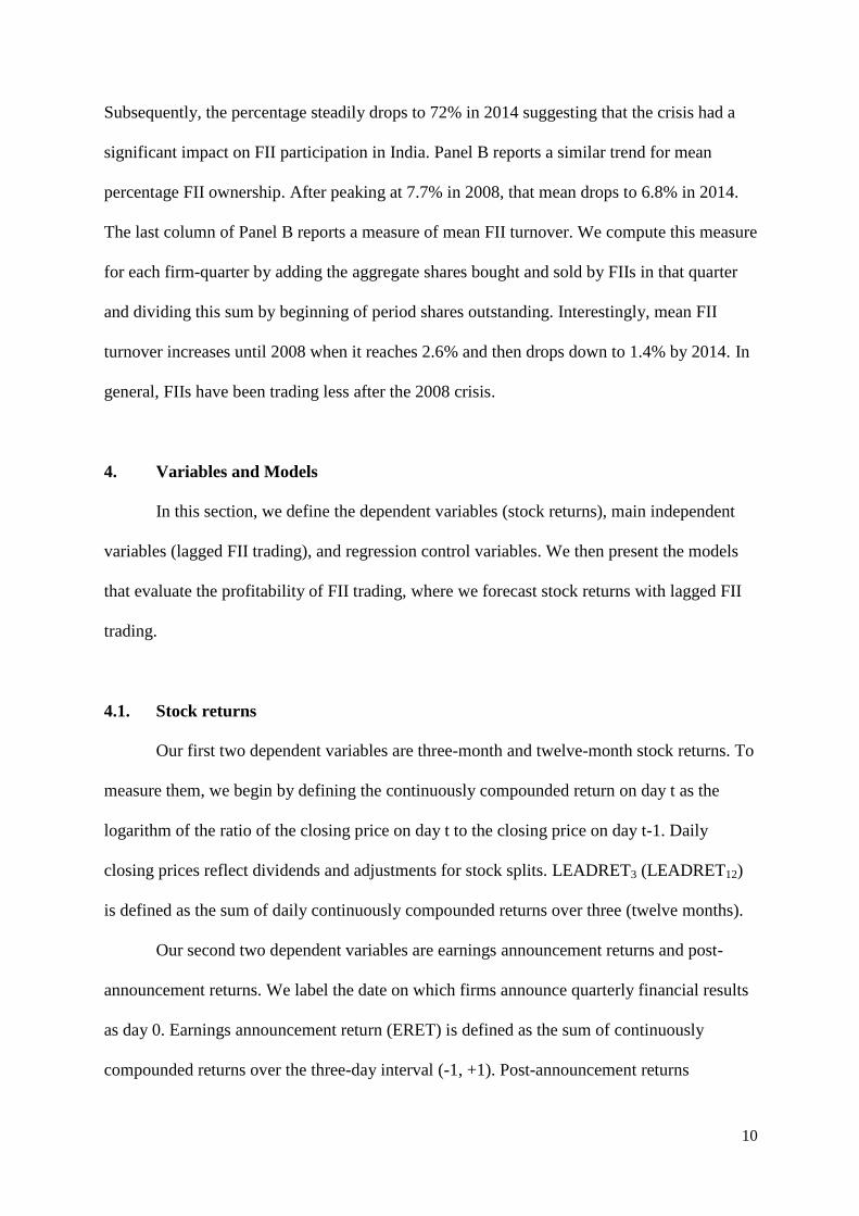
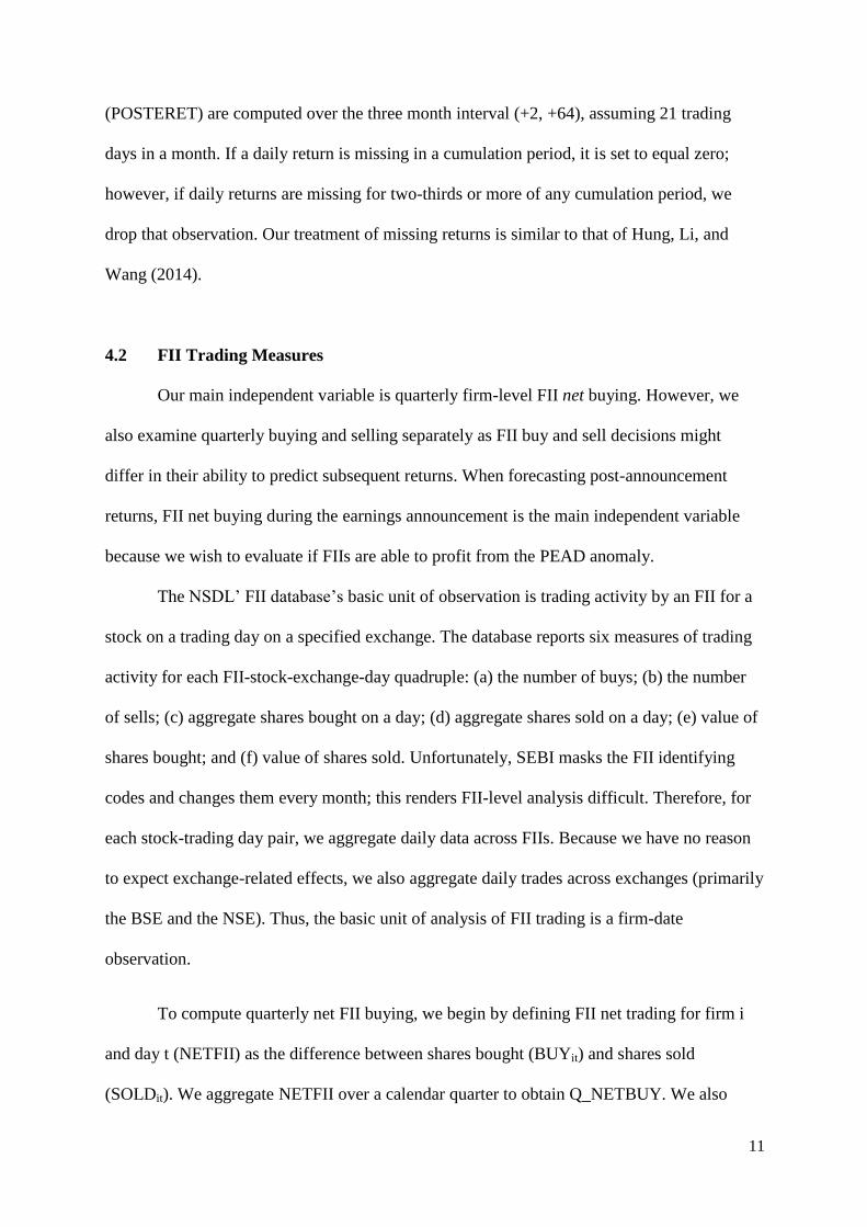
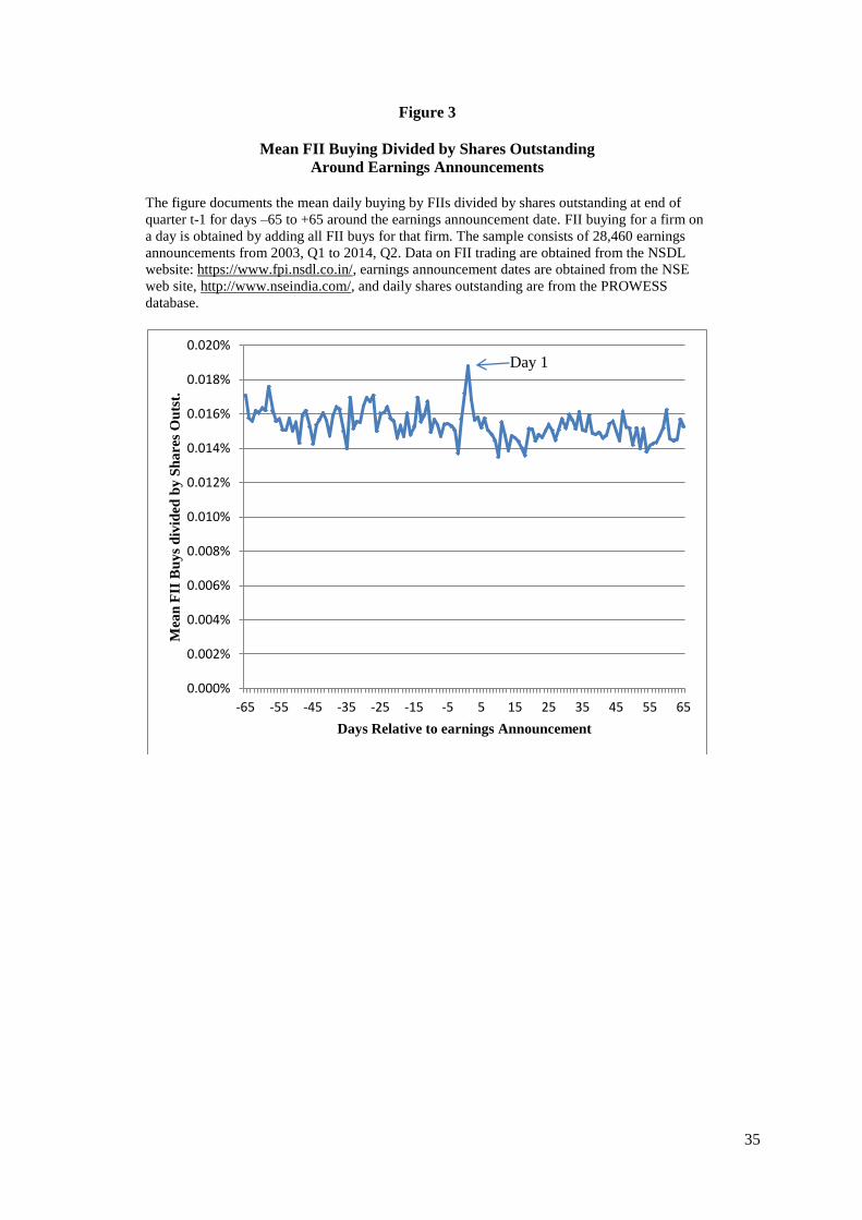
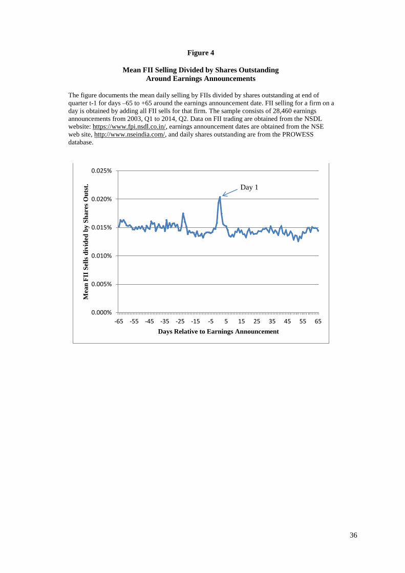
In Figure 3 and 4, we plot the mean daily FII buying and selling (both as a percentage
of daily shares outstanding) separately. Again, we observe a spike in buying and selling
magnitudes on day 1, with a more pronounced spike for selling activity. Table 6 contains

23
volume and FII trading data for days –9 to +9. The numbers confirm the visual information
provided by the plots: days 0 and 1 represent the peak in trading activity for the market and
FIIs in the 19-day interval.
Table 7 relates unexpected earnings to market-adjusted returns before, during, and
after earnings announcements. We divide sample firms in each quarter into four portfolios
based on the distribution of unexpected earnings (UE) in the previous quarter. Recall that UE
is the difference between EPS in quarter t and EPS from quarter t-4, divided by closing price
on day -2. Using last quarter’s UE ensures that the UE distribution is public knowledge on the
date from which returns are cumulated. Next, for each firm-quarter, we compute the
cumulative return over three horizons: days (-64, -2), (-1, +1), and (+2, +64). Averaging
cumulative returns over firms in event-time produces a portfolio cumulative return (CR) for
each UE portfolio and each of the three horizons. Cumulative market-adjusted returns are
computed similarly. Cumulative abnormal returns (CAR) are defined as the difference
between the portfolio-level CR and the market-level CR.
Columns (1) and (2) of Table 7 contain the mean and median values of UE for the
four quartiles. The mean (median) UE spread is 17.9% (7.7%) and is statistically significant
at conventional levels based on a t-test (Wilcoxon Z test). The next four columns contain
evidence on the relation between UE and pre- and during-announcement CARs. Consistent
with prior research, pre-announcement CARs are significantly higher for the high UE quartile
compared to the low UE quartile; the mean (median) difference is 12.6% (10.9%) and
statistically significant. This supports the idea that markets anticipate the sign of future
earnings surprises; that is prices lead earnings (Beaver, Lambert, and Morse (1980)). UE is
also positively correlated with earnings announcement returns; the mean spread between the
high and low UE quartiles is 3.7%.
24
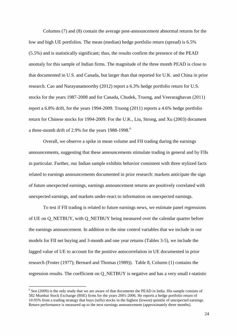
Columns (7) and (8) contain the average post-announcement abnormal returns for the
low and high UE portfolios. The mean (median) hedge portfolio return (spread) is 6.5%
(5.5%) and is statistically significant; thus, the results confirm the presence of the PEAD
anomaly for this sample of Indian firms. The magnitude of the three month PEAD is close to
that documented in U.S. and Canada, but larger than that reported for U.K. and China in prior
research. Cao and Narayanamoorthy (2012) report a 6.3% hedge portfolio return for U.S.
stocks for the years 1987-2008 and for Canada, Chudek, Truong, and Veeraraghavan (2011)
report a 6.8% drift, for the years 1994-2009. Truong (2011) reports a 4.6% hedge portfolio
return for Chinese stocks for 1994-2009. For the U.K., Liu, Strong, and Xu (2003) document
a three-month drift of 2.9% for the years 1988-1998.6
Overall, we observe a spike in mean volume and FII trading during the earnings
announcements, suggesting that these announcements stimulate trading in general and by FIIs
in particular. Further, our Indian sample exhibits behavior consistent with three stylized facts
related to earnings announcements documented in prior research: markets anticipate the sign
of future unexpected earnings, earnings announcement returns are positively correlated with
unexpected earnings, and markets under-react to information on unexpected earnings.
To test if FII trading is related to future earnings news, we estimate panel regressions
of UE on Q_NETBUY, with Q_NETBUY being measured over the calendar quarter before
the earnings announcement. In addition to the nine control variables that we include in our
models for FII net buying and 3-month and one year returns (Tables 3-5), we include the
lagged value of UE to account for the positive autocorrelation in UE documented in prior
research (Foster (1977); Bernard and Thomas (1989)). Table 8, Column (1) contains the
regression results. The coefficient on Q_NETBUY is negative and has a very small t-statistic
6 Sen (2009) is the only study that we are aware of that documents the PEAD in India. His sample consists of
582 Mumbai Stock Exchange (BSE) firms for the years 2001-2006. He reports a hedge portfolio return of
10.05% from a trading strategy that buys (sells) stocks in the highest (lowest) quintile of unexpected earnings.
Return performance is measured up to the next earnings announcement (approximately three months).
25
of -0.22. Thus, quarterly FII trades are unrelated to subsequent quarterly unexpected earnings.
In and of itself, this does not constitute evidence on the investing skill of FIIs; perhaps their
objective function does not require that they forecast short-term earnings growth.
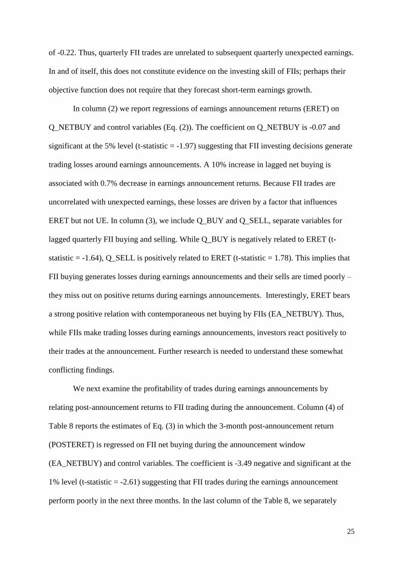
In column (2) we report regressions of earnings announcement returns (ERET) on
Q_NETBUY and control variables (Eq. (2)). The coefficient on Q_NETBUY is -0.07 and
significant at the 5% level (t-statistic = -1.97) suggesting that FII investing decisions generate
trading losses around earnings announcements. A 10% increase in lagged net buying is
associated with 0.7% decrease in earnings announcement returns. Because FII trades are
uncorrelated with unexpected earnings, these losses are driven by a factor that influences
ERET but not UE. In column (3), we include Q_BUY and Q_SELL, separate variables for
lagged quarterly FII buying and selling. While Q_BUY is negatively related to ERET (t-
statistic = -1.64), Q_SELL is positively related to ERET (t-statistic = 1.78). This implies that
FII buying generates losses during earnings announcements and their sells are timed poorly –
they miss out on positive returns during earnings announcements. Interestingly, ERET bears
a strong positive relation with contemporaneous net buying by FIIs (EA_NETBUY). Thus,
while FIIs make trading losses during earnings announcements, investors react positively to
their trades at the announcement. Further research is needed to understand these somewhat
conflicting findings.
We next examine the profitability of trades during earnings announcements by
relating post-announcement returns to FII trading during the announcement. Column (4) of
Table 8 reports the estimates of Eq. (3) in which the 3-month post-announcement return
(POSTERET) is regressed on FII net buying during the announcement window
(EA_NETBUY) and control variables. The coefficient is -3.49 negative and significant at the
1% level (t-statistic = -2.61) suggesting that FII trades during the earnings announcement
perform poorly in the next three months. In the last column of the Table 8, we separately

26
examine the performance of FII buys and sells (EA_BUY and EA_SELL). Again, EA_BUY
is negatively related to POSTERET (t-statistic = -2.33) and EA_SELL is positively related to
POSTERET (t-statistic = 2.52).
The presence of the PEAD anomaly reported in table 7 would suggest that FIIs could
profit by executing trades on earnings announcement dates in the direction of the sign of UE.
In untabulated work, we examine this possibility, by estimating panel regressions of
EA_NETBUY on UE and the nine control variables defined in section 4. Interestingly, the
coefficient on UE is small and negative (-0.0004) and not significant at conventional levels
(p-value = 0.35). In combination with the poor post-announcement performance of FII trades
during earnings announcements, this evidence suggests a failure to capitalize on the PEAD
anomaly.
Overall, the evidence on earnings announcements suggests that FII trades both in the
quarter before earnings announcements and during these announcements are unprofitable.
These findings confirm the general tendency of FII trades to be associated with poor medium-
term performance. Additionally, based on their announcement date trades FIIs appear to miss
the opportunity to profit from the post-earnings announcement drift.
6. Conclusions
This study presents evidence that Foreign Institutional Investor (FII) trades are
unprofitable. Portfolios of stocks that are formed based on positive, zero, and negative FII
quarterly net buying yield average quarterly returns of 1.6%, 3.8%, and 2.4%, respectively.
This suggests that investing in stocks in which FIIs do not trade yields superior returns to
those in which they trade. Further, their sells perform better than their buys. Panel regressions
of 3-month and 12-month returns on lagged quarterly FII net buying and several firm
characteristics establish that poor FII performance holds in a multivariate setting. The poor

27
performance is magnified when FIIs trade in small stocks and when they trade more
frequently than normal. We also find that their quarterly trades are negatively associated with
returns during earnings announcement dates. Further, their trades during the announcements
also generate poor performance in the three-month post-announcement period. Collectively,
the evidence leads us to conclude that FIIs in India do not behave like informed investors.
Our findings lead to the question of why FIIs perform poorly in the Indian market.
The first possibility is that FIIs are either not smart or are overconfident. The evidence that
their losses are magnified when they trade more frequently suggests that overconfidence is a
partial explanation. A second explanation is that other investors perceive FIIs as smart money
and follow /mimic their trades. This herding in turn could lead to prices overshooting true
values and subsequently reversing.7 A third possibility is that FIIs are global investors who
are willing to accept losses in Indian markets some of the time because some of their Indian
trades are executed to rebalance global portfolios and thus reduce risk. A fourth possibility is
that FIIs might be conduits for Indian funds routed back to India via foreign countries.
Because some of these funds may represent income on which taxes have been avoided, FIIs
might be willing to accept trading losses as the benefit from tax avoidance exceeds these
losses. Lastly, the desire to increase or maintain corporate control might cause some FIIs to
behave like long-term investors and accept short-term losses. Disentangling these alternate
explanations would be a very interesting subject for future research. This paper only takes the
first step in understanding FII flows into India and raises more research possibilities.
7 The idea that other investors will mimic FIIs (even though they may not be smart) becomes especially relevant
during earnings announcements. This is because earnings announcements serve as focal points. Schelling (1960)
illustrates the idea of a focal point in coordination games through an abundance of examples. He shows that any
aspect of the problem that has an innate saliency can serve as a potential focal point. The problem before agents
is that even without direct communication and with interests that are not zero-sum but not fully aligned either,
they need to coordinate their actions, for which they need to coordinate expectations. An anticipated earnings
announcement is a natural focal point for market participants.

28
References
Acharya, V., R. Anshuman, and K. Kumar. 2014. Foreign fund flows and stock returns:
Evidence from India. Working Paper, New York University.
Ali, A., C. Durtschi, B. Lev, and M. Trombley. 2004. Changes in institutional ownership and
subsequent earnings announcement abnormal returns. Journal of Accounting, Auditing
and Finance 3: 221-248.
Bae, S., J. Min, and S. Jung. 2011. Trading behavior, performance, and stock preference of
foreigners, local Institutions, and individual investors: Evidence from the Korean stock
market. Asia-Pacific Journal of Financial Studies 40: 199-239.
Baker, M., L. Litov, J. Wachter, and J. Wurgler. 2010. Can mutual fund managers pick
stocks? Evidence from trades prior to earnings announcements. Journal of Financial
and Quantitative Analysis 45: 1111-1131.
Barber, B. and T. Odean. 2000. Trading is hazardous to your wealth: The common stock
investment performance of individual investors. Journal of Finance 55: 773-806.
Beaver, W. R. Lambert, and D. Morse. 1980. The information content of security prices.
Journal of Accounting and Economics 2: 3-28.
Bennett, J., R. Sias, and L. Starks. 2003. Greener pastures and the impact of dynamic
institutional preferences. Review of Financial Studies16:1203-1238.
Berkman, H. and M. McKenzie.2012. Earnings announcements: Good news for institutional
investors and short sellers. The Financial Review 47: 91-113.
Bernard, V. and J. Thomas. 1989. Post-earnings-announcement drift: Delayed price response
or risk premium? Journal of Accounting Research 27: 1-36.
Brennan, M. and H. Cao. 1997. International portfolio investment flows. Journal of Finance
52: 1851-1880.
29
Bushee, B. and T. Goodman. 2007. Which institutional investors trade based on private
information about earnings and returns? Journal of Accounting Research 45: 289-321.
Cai, F., and L. Zheng. 2004. Institutional trading and stock Returns. Finance Research Letters
1:178-189.
Campbell, J., T. Ramadorai, and A. Schwartz. 2009. Caught on tape: Institutional
trading, stock returns, and earnings announcements. Journal of Financial Economics
92: 66-91.
Cao, S. and G. Narayanamoorthy. 2012. Earnings volatility, post–earnings announcement
drift, and trading frictions. Journal of Accounting Research 50: 41-74.
Choe, H., B. Kho, and R. Stulz. 2005. Do domestic investors have an edge? The trading
experience of foreign investors in Korea. Review of Financial Studies 18: 795-829.
Chudek, M., C. Truong, and M. Veeraraghavan. 2011. Is trading on earnings surprises a
profitable strategy? Canadian evidence. Journal of International Financial Markets
Institutions & Money 21: 832-850.
Daniel, K. and D. Hirshleifer. 2015. Overconfident investors, predictable returns, and
excessive trading. Journal of Economic Perspectives 29: 61-88.
Del Guercio, D. 1996. The distorting effect of the prudent-man laws on institutional equity
investment. Journal of Financial Economics 40: 31-62.
Dvorak, T. 2005. Do domestic investors have an informational advantage? Evidence from
Indonesia. Journal of Finance 60: 817-839.
Economic Times. July 1, 2014. Promoter-banker-FII nexus under scanner for P-Note abuse.
Economic Times. Retrieved from http://articles.economictimes.indiatimes.com/2014-
07-01/news/51002682_1_offshore-derivative-instruments-entities-registered-fiis
Edelen, R., O. Inze, and G. Kadlec. 2015. Institutional investors and stock return anomalies.
Journal of Financial Economics Forthcoming.

30
Eom, Y., J. Hahn, and W. Sohn. 2010. Post-earnings announcement drift and foreign
investors’ trading behaviour in Korea. Working Paper, Hansung University.
Foster, G. 1977. Quarterly accounting data: Time-series properties and predictive-ability
results. The Accounting Review 52: 1-21.
Gompers, P. and A. Metrick. 2001. Institutional investors and equity prices. Quarterly
Journal of Economics 116: 229-259.
Griffin, J., T. Shu, and S. Topaloglu. 2012. Examining the dark side of financial markets:
Do institutions trade on information from investment bank connections? Review of
Financial Studies 25: 2155-2188.
Grinblatt, M., and M. Keloharju. 2000. The investor behavior and performance of various
investor types: A study of Finland’s unique data set. Journal of Financial Economics
55: 43-67.
Hendershott, T., D. Livdan, and N. Schurhoff. 2014. Are institutions informed about news?
Journal of Financial Economics Forthcoming.
Huang, R., and C. Shiu. 2009. Local effects of foreign ownership in an emerging financial
market: Evidence from qualified foreign institutional investors in Taiwan. Financial
Management Autumn: 567-202.
Hung, M., X. Li, and S. Wang. 2014. Post-earnings-announcement drift in global markets:
Evidence from an information shock. Review of Financial Studies. Forthcoming.
International Organization of Securities Commissions (IOSCO). 2012. Report of the
Emerging Markets Committee on Development and Regulation of Institutional
Investors in Emerging Markets.
https://www.iosco.org/library/pubdocs/pdf/IOSCOPD384.pdf
Kang, J., and R. Stulz. 1997. Why is there a home bias? An analysis of foreign portfolio
equity ownership in Japan. Journal of Financial Economics 46: 3-28.

31
Ke, B. and K. Petroni. 2004. How informed are actively trading institutional investors?
Evidence from their trading behavior before a break in a string of consecutive earnings
increases. Journal of Accounting Research 42: 895-927.
Liu, W., N. Strong, and X. Xu. 2003. Post-earnings announcement drift in the UK. European
Financial Management 9: 89-116.
Lo, A. and J. Wang. 2000. Trading volume: Definitions, data analysis, and implications of
portfolio theory. Review of Financial Studies 13: 257-300.
Nofsinger, J., and R. Sias. 1999. Herding and feedback trading by institutional and individual
investors. Journal of Finance 54: 2263-2295.
Odean, T. 1998. Volume, volatility, price, and profit when all traders are above average.
Journal of Finance 53: 1887-1934.
Parikh, G. 2014. Handbook of Indian securities. Bloomsbury Publishing. New Delhi.
Park, T., Y. Lee, and K. Song. 2013. Informed trading before earnings shock. Working Paper,
Sungkyunkwan University.
Puckett, A. and X.Yan. 2011. The interim trading skills of institutional investors. Journal of
Finance 66, 601-633.
Schelling, T. 1960. The Strategy of Conflict. Harvard University Press. Cambridge, MA.
Seasholes, M. 2003. Smart foreign traders in emerging markets. Working Paper, Harvard
University.
Sen, K. 2009. Earnings surprise and sophisticated investor preferences in India. Journal of
Contemporary Accounting & Economics 5: 1-19.
Sias, R. 2004. Institutional Herding. Review of Financial Studies 17:165–206.
Truong, C. 2011. Post-earnings announcement abnormal return in the Chines Equity market.
Journal of International Financial Markets Institutions & Money 21: 637-661.

32
Yan, X. and Z. Zhang. 2009. Institutional investors and equity returns: Are short-term
institutions better informed? Review of Financial Studies 22: 893-924.
33
Figure 1
The figure tracks the value of 1₹ invested on March 31, 2003 in three portfolios of stocks: stocks in which FIIs
are net buyers in a quarter (net buy portfolio), stocks in which they did not trade during the quarter (no trade
portfolio), and stocks in which FIIs are net sellers (net sell portfolio). Portfolios are formed at the end of each
quarter and one-quarter ahead value-weighted returns are calculated, with weights equalling the market
capitalization at the end of the quarter in which portfolios are formed. Quarterly returns are computed by
summing continuously compounded daily returns. We then calculate the product of 1 plus each portfolio return
over time to arrive at the future value of ₹1 at the end of the third quarter of 2014. Data on daily returns are
obtained from the PROWESS database. Data on FII trading are obtained from the NSDL website:
https://www.fpi.nsdl.co.in/
0
1
2
3
4
5
6
7
8
20
03
.03
20
04
.03
20
05
.03
20
06
.03
20
07
.03
20
08
.03
20
09
.03
20
10
.03
20
11
.03
20
12
.03
20
13
.03
20
14
.03
FII Sells No Trade FII Buys
34
Figure 2
Mean Volume / Shares Outstanding around Earnings Announcements
The figure documents mean daily trading volume divided by shares outstanding for days -65 to +65
around the earnings announcement date. The sample consists of 28,460 earnings announcements
from 2003, Q1 to 2014, Q2. Data on daily volume and shares outstanding are obtained from the
PROWESS database and earnings announcement dates are obtained from the NSE web site,
http://www.nseindia.com/.
0.000%
0.050%
0.100%
0.150%
0.200%
0.250%
0.300%
0.350%
0.400%
-65 -55 -45 -35 -25 -15 -5 5 15 25 35 45 55 65
Mea
n V
olu
me/
Sh
are
s O
uts
.
Days Relative to Earnings Announcement
Day 0
35
Figure 3
Mean FII Buying Divided by Shares Outstanding
Around Earnings Announcements
The figure documents the mean daily buying by FIIs divided by shares outstanding at end of
quarter t-1 for days –65 to +65 around the earnings announcement date. FII buying for a firm on
a day is obtained by adding all FII buys for that firm. The sample consists of 28,460 earnings
announcements from 2003, Q1 to 2014, Q2. Data on FII trading are obtained from the NSDL
website: https://www.fpi.nsdl.co.in/, earnings announcement dates are obtained from the NSE
web site, http://www.nseindia.com/, and daily shares outstanding are from the PROWESS
database.
0.000%
0.002%
0.004%
0.006%
0.008%
0.010%
0.012%
0.014%
0.016%
0.018%
0.020%
-65 -55 -45 -35 -25 -15 -5 5 15 25 35 45 55 65
Mea
n F
II B
uy
s d
ivid
ed b
y S
ha
res
Ou
tst.
Days Relative to earnings Announcement
Day 1
36
Figure 4
Mean FII Selling Divided by Shares Outstanding
Around Earnings Announcements
The figure documents the mean daily selling by FIIs divided by shares outstanding at end of
quarter t-1 for days –65 to +65 around the earnings announcement date. FII selling for a firm on a
day is obtained by adding all FII sells for that firm. The sample consists of 28,460 earnings
announcements from 2003, Q1 to 2014, Q2. Data on FII trading are obtained from the NSDL
website: https://www.fpi.nsdl.co.in/, earnings announcement dates are obtained from the NSE
web site, http://www.nseindia.com/, and daily shares outstanding are from the PROWESS
database.
0.000%
0.005%
0.010%
0.015%
0.020%
0.025%
-65 -55 -45 -35 -25 -15 -5 5 15 25 35 45 55 65
Mea
n F
II S
ells
div
ided
by
Sh
are
s O
uts
t.
Days Relative to Earnings Announcement
Day 1
37
Table 1
Sample Selection and Yearly Distribution
We conduct two sets of analyses relating FII trading to subsequent stock returns. In the first set of tests, we predict
3-month and 12 month returns with FII trading; in the second set, we predict earnings announcement returns. Panel
A reports the screens used to arrive at the final samples for the two set of tests. The initial sample consists of
observations with non-missing data for quarterly FII trading and contemporaneous stock returns. The sample
period is from 2003, Q1 to 2014, Q2. Panel B reports the yearly frequencies of total number of firm-quarters, firm-
quarters with zero FII ownership, and firm-quarters with non-zero FII ownership. The panel also reports the yearly
percentages of firms with FII ownership, mean FII ownership, and mean turnover. Data on FII trading are obtained
from the NSDL website: https://www.fpi.nsdl.co.in/. Stock returns, quarterly ownership data, and data items used
to define control variables are from the PROWESS database. Data on earnings announcement dates are from the
NSE website, www.nseindia.com. Variable definitions are contained in Table 2.
Panel A: Sample Selection
Firms Firm-quarters
Initial Sample: 1,846 57,596
Less:
Missing data for control variables 10,926
Missing data for FII ownership 156
Sample for 3 month return and 12 month return tests 1,696 46,514
Less:
Missing earnings announcement dates 14,655
Missing unexpected earnings 1,955
Missing post- earnings announcement returns 1,084
Sample for earnings announcement tests 1,535 28,460
Panel B: Frequency Distribution of firm-quarters by FII Ownership and Year
Year
# of firm-
quarters
Zero FII
Ownership
Non-Zero
FII
ownership
% of Obs.
With FII
ownership
Mean %
FII
ownership
Mean FII
(Buys +
Sells)/Shares
Outstanding
2003 2,511 1,050 1,461 58% 2.8% 0.7%
2004 2,526 838 1,688 67% 4.2% 1.1%
2005 2,826 653 2,173 77% 5.9% 1.7%
2006 3,036 637 2,399 79% 7.3% 2.2%
2007 3,372 699 2,673 79% 8.3% 2.7%
2008 4,108 840 3,268 80% 7.7% 2.6%
2009 4,618 1,062 3,556 77% 6.4% 1.9%
2010 4,763 1,099 3,664 77% 6.5% 2.1%
2011 5,131 1,329 3,802 74% 6.4% 1.7%
2012 5,510 1,610 3,900 71% 6.0% 1.5%
2013 5,465 1,599 3,866 71% 6.4% 1.4%
2014 2,648 749 1,899 72% 6.8% 1.6%
Total 46,514 12,165 34,349
38
Table 2
Descriptive Statistics
This table presents descriptive statistics. QBUY (QSELL) is the sum of all FII buys (sells) for a firm over a quarter divided by the shares outstanding at the
beginning of that quarter. Q_NETBUY is the difference between sum of quarterly buys and the sum of quarterly sells, divided by the shares outstanding at the
beginning of the quarter. EA_NETBUY is the net FII buying during the earnings announcement interval, (-1, +1). FIIP is the percentage FII ownership at the end of
each quarter. Returns over various horizons are computed by summing continuously compounded returns over those horizons. LEADRET3 (LEADRET12) is the
three-month (twelve-month) return following the quarter over which Q_NETBUY is measured. ERET is the earnings announcement return over days (-1, +1)
relative to the earnings announcement date. MRET is the market return over days (-1, +1), with the percentage changes in the CNX Nifty Index employed to
measure market return. UE equals earnings per share for quarter t less earnings per share for quarter t-4 divided by closing price on day -2 relative to the earnings
announcement for quarter t-1. We employ 9 control variables in our analyses: LAGRET3, LAGRET9, MCAP, PRC, BM, DIVY, AGE, QSTD, and QTO.
LAGRET3 is the return over the 3 months prior to the quarter over which FII trading is measured. LAGRET9 is the return measured over the 9 months prior to the
3-month period over which LAGRET3 is measured. MCAP is the share price times shares outstanding measured at the beginning of the quarter. PRC is the share
price at the beginning of the quarter. BM is defined as book value of equity divided by MCAP. Book value of equity is measured either on the date MCAP is
measured or on the year end date of the most recently concluded fiscal year. DIVY is the annual cash dividend paid in the fiscal year for which book value of equity
is measured, divided by MCAP. AGE is the number of years since the year of incorporation. QSTD is the standard deviation of monthly returns over the twelve
months before the quarter in which FII trading is measured. QTO is the average monthly volume divided by shares outstanding over the three months before the
quarter in which FII trading is measured. Data on FII trading are obtained from the NSDL website: https://www.fpi.nsdl.co.in/. Quarterly FII ownership, daily stock
returns, prices, and shares outstanding, quarterly earnings per share, and data items used to define control variables are from the PROWESS database. Earnings
announcement dates are from the NSE website. All variables are winsorized at the 1% and 99% levels.
# obs. Mean Median Std. Dev. Q1 Q3
QBUY 46,514 0.9% 0.0% 2.1% 0.0% 0.7%
QSELL 46,514 0.9% 0.0% 1.9% 0.0% 0.7%
Q_NETBUY 46,514 0.1% 0.0% 1.2% 0.0% 0.0%
EA_NETBUY 28,460 -10,367 0 915,944 0 0
LEADRET3 46,221 2.7% 1.7% 29.6% -14.5% 19.6%
LEADRET12 42,694 7.8% 8.3% 62.0% -28.7% 47.1%
ERET 28,460 -0.3% -0.6% 6.6% -4.0% 2.9%
MRET 28,460 -0.01% -0.03% 2.9% -1.5% 1.4%
UE 28,212 -1.1% 0.1% 11.29% -1.36% 1.03%
FIIP 46,514 6.3% 1.8% 9.0% 0.0% 9.7%
LAGRET3 46,514 1.3% 0.6% 29.3% -15.4% 17.8%
LAGRET9 46,514 2.6% 2.1% 54.4% -29.3% 35.4%
39
MCAP (million ₹) 46,514 31545.1 3136.5 99124.7 828.5 14940.3
PRC (₹) 46,514 215.8 83.5 372.7 28.5 229.3
BM 46,514 1.0 0.7 1.9 0.3 1.4
DIVY 46,514 1.7% 1.0% 2.2% 0.0% 2.5%
AGE (years) 46,514 32.5 25.0 22.2 17.0 43.0
QSTD 46,514 15.0% 13.6% 7.0% 9.9% 18.8%
QTO 46,514 5.1% 1.9% 8.6% 0.7% 5.3%
40
Table 3
Determinants of FII Trading
This table reports the results of panel regressions of net FII buying on nine stock characteristics. The
sample period is from 2003, Q1 to 2014, Q2. Q_NETBUY is the difference between sum of quarterly buys
and the sum of quarterly sells, divided by the shares outstanding at the beginning of the quarter. Data on FII
trading are obtained from the NSDL website: https://www.fpi.nsdl.co.in/. LAGRET3 is the return over the
3 months prior to the quarter over which FII trading is measured. LAGRET9 is the return measured over
the 9 months prior to the 3-month period over which LAGRET3 is measured. MCAP is the share price
times shares outstanding measured at the beginning of the quarter. PRC is the share price at the beginning
of the quarter. BM is defined as book value of equity divided by MCAP. Book value of equity is measured
either on the date MCAP is measured or on the year end date of the most recently concluded fiscal year.
DIVY is the annual cash dividend paid in the fiscal year for which book value of equity is measured,
divided by MCAP. AGE is the number of years since the year of incorporation. QSTD is the standard
deviation of monthly returns over the twelve months before the quarter in which FII trading is measured.
QTO is the average monthly volume divided by shares outstanding over the three months before the quarter
in which FII trading is measured. MCAP, PRC, AGE, QSTD, and QTO are expressed in natural logarithms.
All regressions include firm and quarter fixed effects and standard errors are adjusted for two-way
clustering. All variables are winsorized at the 1% and 99% levels. Quarterly FII ownership, stock returns,
and data items used to define control variables are from the PROWESS database.
Dependent Variable: Q_NETBUY
Coef. t-stat.
Intercept 0.001 7.25
(0.00)
LAGRET3 0.004 9.19
(0.00)
LAGRET9 0.002 9.07
(0.00)
MCAP 0.001 3.93
(0.00)
PRC -0.001 -3.98
(0.00)
BM 0.000 -1.84
(0.07)
DIVY -0.032 -6.78
(0.00)
AGE -0.002 -1.95
(0.05)
QSTD -0.001 -2.51
(0.01)
QTO 0.000 1.38
(0.17)
Firm Effects
Yes
Quarter Effects
Yes
# of obs.
46,509
Adj. R2
3.06%
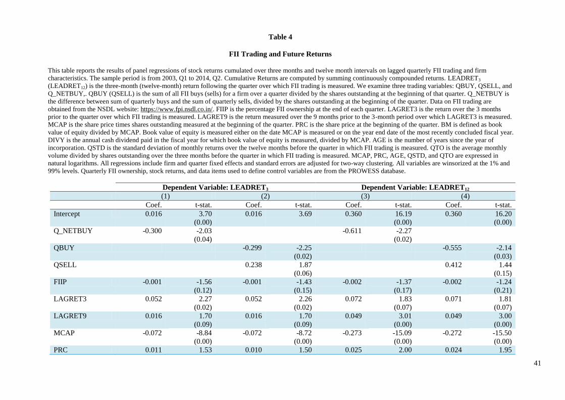
41
Table 4
FII Trading and Future Returns
This table reports the results of panel regressions of stock returns cumulated over three months and twelve month intervals on lagged quarterly FII trading and firm
characteristics. The sample period is from 2003, Q1 to 2014, Q2. Cumulative Returns are computed by summing continuously compounded returns. LEADRET3
(LEADRET12) is the three-month (twelve-month) return following the quarter over which FII trading is measured. We examine three trading variables: QBUY, QSELL, and
Q_NETBUY,. QBUY (QSELL) is the sum of all FII buys (sells) for a firm over a quarter divided by the shares outstanding at the beginning of that quarter. Q_NETBUY is
the difference between sum of quarterly buys and the sum of quarterly sells, divided by the shares outstanding at the beginning of the quarter. Data on FII trading are
obtained from the NSDL website: https://www.fpi.nsdl.co.in/. FIIP is the percentage FII ownership at the end of each quarter. LAGRET3 is the return over the 3 months
prior to the quarter over which FII trading is measured. LAGRET9 is the return measured over the 9 months prior to the 3-month period over which LAGRET3 is measured.
MCAP is the share price times shares outstanding measured at the beginning of the quarter. PRC is the share price at the beginning of the quarter. BM is defined as book
value of equity divided by MCAP. Book value of equity is measured either on the date MCAP is measured or on the year end date of the most recently concluded fiscal year.
DIVY is the annual cash dividend paid in the fiscal year for which book value of equity is measured, divided by MCAP. AGE is the number of years since the year of
incorporation. QSTD is the standard deviation of monthly returns over the twelve months before the quarter in which FII trading is measured. QTO is the average monthly
volume divided by shares outstanding over the three months before the quarter in which FII trading is measured. MCAP, PRC, AGE, QSTD, and QTO are expressed in
natural logarithms. All regressions include firm and quarter fixed effects and standard errors are adjusted for two-way clustering. All variables are winsorized at the 1% and
99% levels. Quarterly FII ownership, stock returns, and data items used to define control variables are from the PROWESS database.
Dependent Variable: LEADRET3 Dependent Variable: LEADRET12
(1) (2) (3) (4)
Coef. t-stat. Coef. t-stat. Coef. t-stat. Coef. t-stat.
Intercept 0.016 3.70
(0.00)
0.016 3.69 0.360 16.19
(0.00)
0.360 16.20
(0.00)
Q_NETBUY -0.300 -2.03
(0.04)
-0.611 -2.27
(0.02)
QBUY -0.299 -2.25
(0.02)
-0.555 -2.14
(0.03)
QSELL 0.238 1.87
(0.06)
0.412 1.44
(0.15)
FIIP -0.001 -1.56
(0.12)
-0.001 -1.43
(0.15)
-0.002 -1.37
(0.17)
-0.002 -1.24
(0.21)
LAGRET3 0.052 2.27
(0.02)
0.052 2.26
(0.02)
0.072 1.83
(0.07)
0.071 1.81
(0.07)
LAGRET9 0.016 1.70
(0.09)
0.016 1.70
(0.09)
0.049 3.01
(0.00)
0.049 3.00
(0.00)
MCAP -0.072 -8.84
(0.00)
-0.072 -8.72
(0.00)
-0.273 -15.09
(0.00)
-0.272 -15.50
(0.00)
PRC 0.011 1.53 0.010 1.50 0.025 2.00 0.024 1.95
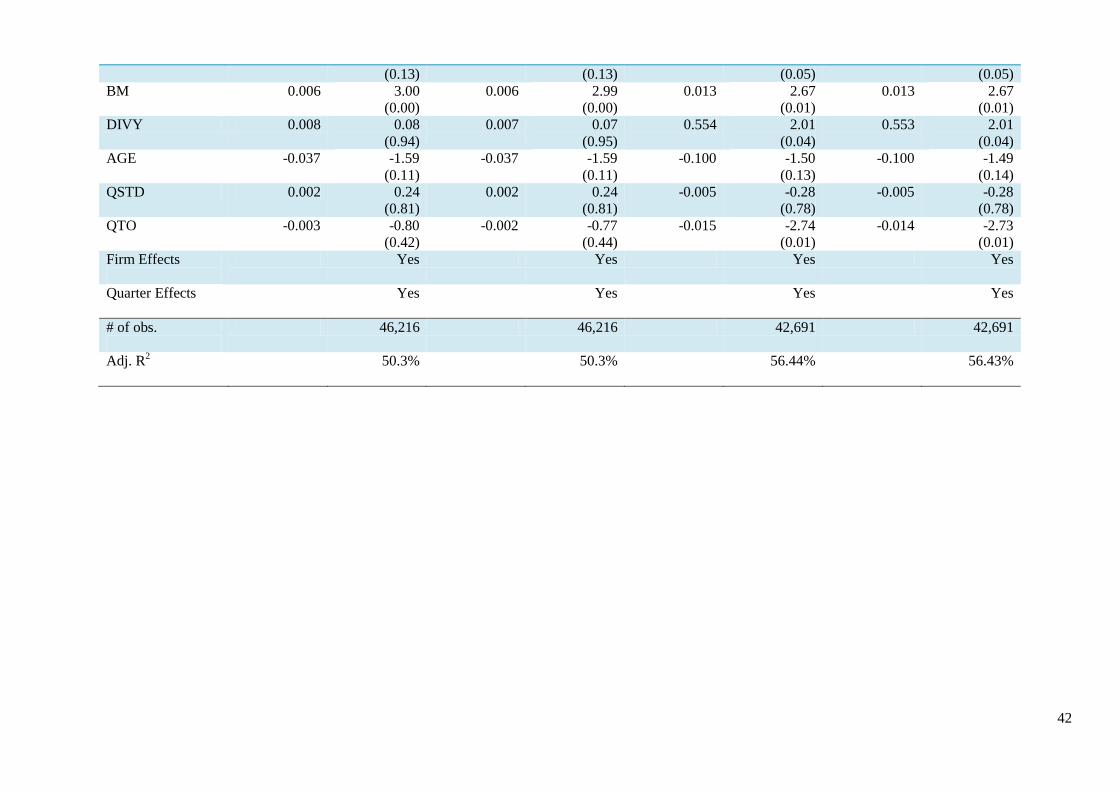
42
(0.13) (0.13) (0.05) (0.05)
BM 0.006 3.00
(0.00)
0.006 2.99
(0.00)
0.013 2.67
(0.01)
0.013 2.67
(0.01)
DIVY 0.008 0.08
(0.94)
0.007 0.07
(0.95)
0.554 2.01
(0.04)
0.553 2.01
(0.04)
AGE -0.037 -1.59
(0.11)
-0.037 -1.59
(0.11)
-0.100 -1.50
(0.13)
-0.100 -1.49
(0.14)
QSTD 0.002 0.24
(0.81)
0.002 0.24
(0.81)
-0.005 -0.28
(0.78)
-0.005 -0.28
(0.78)
QTO -0.003 -0.80
(0.42)
-0.002 -0.77
(0.44)
-0.015 -2.74
(0.01)
-0.014 -2.73
(0.01)
Firm Effects
Yes Yes Yes Yes
Quarter Effects
Yes Yes Yes Yes
# of obs.
46,216 46,216 42,691 42,691
Adj. R2
50.3% 50.3% 56.44% 56.43%
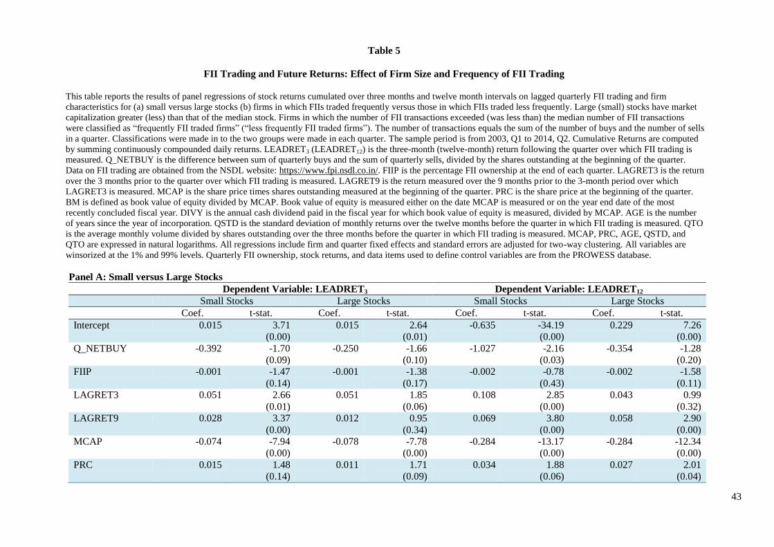
43
Table 5
FII Trading and Future Returns: Effect of Firm Size and Frequency of FII Trading
This table reports the results of panel regressions of stock returns cumulated over three months and twelve month intervals on lagged quarterly FII trading and firm
characteristics for (a) small versus large stocks (b) firms in which FIIs traded frequently versus those in which FIIs traded less frequently. Large (small) stocks have market
capitalization greater (less) than that of the median stock. Firms in which the number of FII transactions exceeded (was less than) the median number of FII transactions
were classified as “frequently FII traded firms” (“less frequently FII traded firms”). The number of transactions equals the sum of the number of buys and the number of sells
in a quarter. Classifications were made in to the two groups were made in each quarter. The sample period is from 2003, Q1 to 2014, Q2. Cumulative Returns are computed
by summing continuously compounded daily returns. LEADRET3 (LEADRET12) is the three-month (twelve-month) return following the quarter over which FII trading is
measured. Q_NETBUY is the difference between sum of quarterly buys and the sum of quarterly sells, divided by the shares outstanding at the beginning of the quarter.
Data on FII trading are obtained from the NSDL website: https://www.fpi.nsdl.co.in/. FIIP is the percentage FII ownership at the end of each quarter. LAGRET3 is the return
over the 3 months prior to the quarter over which FII trading is measured. LAGRET9 is the return measured over the 9 months prior to the 3-month period over which
LAGRET3 is measured. MCAP is the share price times shares outstanding measured at the beginning of the quarter. PRC is the share price at the beginning of the quarter.
BM is defined as book value of equity divided by MCAP. Book value of equity is measured either on the date MCAP is measured or on the year end date of the most
recently concluded fiscal year. DIVY is the annual cash dividend paid in the fiscal year for which book value of equity is measured, divided by MCAP. AGE is the number
of years since the year of incorporation. QSTD is the standard deviation of monthly returns over the twelve months before the quarter in which FII trading is measured. QTO
is the average monthly volume divided by shares outstanding over the three months before the quarter in which FII trading is measured. MCAP, PRC, AGE, QSTD, and
QTO are expressed in natural logarithms. All regressions include firm and quarter fixed effects and standard errors are adjusted for two-way clustering. All variables are
winsorized at the 1% and 99% levels. Quarterly FII ownership, stock returns, and data items used to define control variables are from the PROWESS database.
Panel A: Small versus Large Stocks
Dependent Variable: LEADRET3 Dependent Variable: LEADRET12
Small Stocks Large Stocks Small Stocks Large Stocks
Coef. t-stat. Coef. t-stat. Coef. t-stat. Coef. t-stat.
Intercept 0.015 3.71
(0.00)
0.015 2.64
(0.01)
-0.635 -34.19
(0.00)
0.229 7.26
(0.00)
Q_NETBUY -0.392 -1.70
(0.09)
-0.250 -1.66
(0.10)
-1.027 -2.16
(0.03)
-0.354 -1.28
(0.20)
FIIP -0.001 -1.47
(0.14)
-0.001 -1.38
(0.17)
-0.002 -0.78
(0.43)
-0.002 -1.58
(0.11)
LAGRET3 0.051 2.66
(0.01)
0.051 1.85
(0.06)
0.108 2.85
(0.00)
0.043 0.99
(0.32)
LAGRET9 0.028 3.37
(0.00)
0.012 0.95
(0.34)
0.069 3.80
(0.00)
0.058 2.90
(0.00)
MCAP -0.074 -7.94
(0.00)
-0.078 -7.78
(0.00)
-0.284 -13.17
(0.00)
-0.284 -12.34
(0.00)
PRC 0.015 1.48
(0.14)
0.011 1.71
(0.09)
0.034 1.88
(0.06)
0.027 2.01
(0.04)
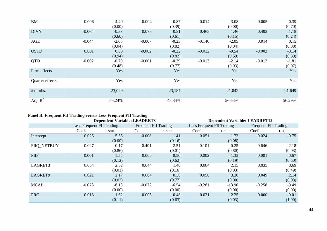
44
BM 0.006 4.49
(0.00)
0.004 0.87
(0.39)
0.014 3.08
(0.00)
0.005 0.39
(0.70)
DIVY -0.064 -0.53
(0.60)
0.075 0.51
(0.61)
0.465 1.46
(0.15)
0.493 1.18
(0.24)
AGE -0.044 -2.05
(0.04)
-0.007 -0.23
(0.82)
-0.140 -2.05
(0.04)
0.014 0.15
(0.88)
QSTD 0.001 0.08
(0.94)
-0.002 -0.22
(0.82)
-0.012 -0.54
(0.59)
-0.003 -0.14
(0.89)
QTO -0.002 -0.70
(0.48)
-0.001 -0.29
(0.77)
-0.013 -2.14
(0.03)
-0.012 -1.81
(0.07)
Firm effects
Yes Yes Yes Yes
Quarter effects
Yes Yes Yes Yes
# of obs.
23,029 23,187 21,042 21,649
Adj. R2
53.24% 48.84% 56.63% 56.29%
Panel B: Frequent FII Trading versus Less Frequent FII Trading
Dependent Variable: LEADRET3 Dependent Variable: LEADRET12
Less Frequent FII Trading Frequent FII Trading Less Frequent FII Trading Frequent FII Trading
Coef. t-stat. Coef. t-stat. Coef. t-stat. Coef. t-stat.
Intercept 0.025 5.55
(0.00)
-0.008 -1.41
(0.16)
-0.051 -1.73
(0.08)
-0.024 -0.75
FIIQ_NETBUY 0.027 0.17
(0.86)
-0.401 -2.51
(0.01)
-0.101 -0.25
(0.80)
-0.646 -2.18
(0.03)
FIIP -0.001 -1.55
(0.12)
0.000 -0.50
(0.62)
-0.002 -1.33
(0.19)
-0.001 -0.67
(0.50)
LAGRET3 0.054 2.52
(0.01)
0.044 1.40
(0.16)
0.084 2.15
(0.03)
0.035 0.69
(0.49)
LAGRET9 0.021 2.17
(0.03)
0.004 0.30
(0.77)
0.056 3.20
(0.00)
0.049 2.14
(0.03)
MCAP -0.073 -8.13
(0.00)
-0.072 -6.54
(0.00)
-0.281 -13.90
(0.00)
-0.258 -9.49
(0.00)
PRC 0.013 1.62
(0.11)
0.005 0.48
(0.63)
0.031 2.25
(0.03)
0.000 -0.01
(1.00)
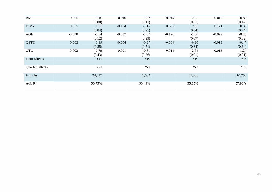
45
BM 0.005 3.16
(0.00)
0.010 1.62
(0.11)
0.014 2.82
(0.01)
0.013 0.80
(0.42)
DIVY 0.025 0.21
(0.84)
-0.194 -1.16
(0.25)
0.632 2.06
(0.04)
0.171 0.33
(0.74)
AGE -0.038 -1.54
(0.12)
-0.037 -1.07
(0.29)
-0.126 -1.80
(0.07)
-0.022 -0.23
(0.82)
QSTD 0.002 0.19
(0.85)
-0.004 -0.37
(0.71)
-0.004 -0.20
(0.84)
-0.013 -0.47
(0.64)
QTO -0.002 -0.79
(0.43)
-0.001 -0.31
(0.76)
-0.014 -2.64
(0.01)
-0.013 -1.24
(0.21)
Firm Effects
Yes Yes Yes Yes
Quarter Effects
Yes Yes Yes Yes
# of obs.
34,677 11,539 31,906 10,790
Adj. R2
50.75% 50.49% 55.85% 57.90%
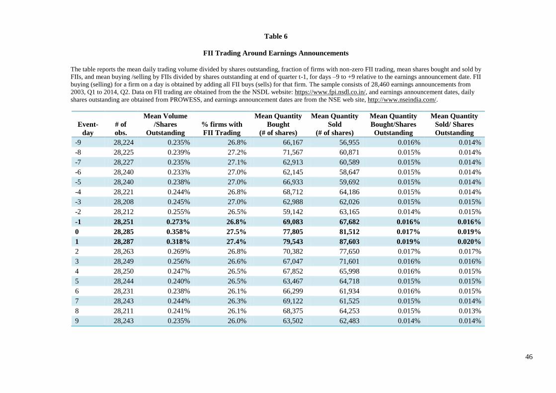
46
Table 6
FII Trading Around Earnings Announcements
The table reports the mean daily trading volume divided by shares outstanding, fraction of firms with non-zero FII trading, mean shares bought and sold by
FIIs, and mean buying /selling by FIIs divided by shares outstanding at end of quarter t-1, for days –9 to +9 relative to the earnings announcement date. FII
buying (selling) for a firm on a day is obtained by adding all FII buys (sells) for that firm. The sample consists of 28,460 earnings announcements from
2003, Q1 to 2014, Q2. Data on FII trading are obtained from the the NSDL website: https://www.fpi.nsdl.co.in/, and earnings announcement dates, daily
shares outstanding are obtained from PROWESS, and earnings announcement dates are from the NSE web site, http://www.nseindia.com/.
Event-
day
# of
obs.
Mean Volume
/Shares
Outstanding
% firms with
FII Trading
Mean Quantity
Bought
(# of shares)
Mean Quantity
Sold
(# of shares)
Mean Quantity
Bought/Shares
Outstanding
Mean Quantity
Sold/ Shares
Outstanding
-9 28,224 0.235% 26.8% 66,167 56,955 0.016% 0.014%
-8 28,225 0.239% 27.2% 71,567 60,871 0.015% 0.014%
-7 28,227 0.235% 27.1% 62,913 60,589 0.015% 0.014%
-6 28,240 0.233% 27.0% 62,145 58,647 0.015% 0.014%
-5 28,240 0.238% 27.0% 66,933 59,692 0.015% 0.014%
-4 28,221 0.244% 26.8% 68,712 64,186 0.015% 0.014%
-3 28,208 0.245% 27.0% 62,988 62,026 0.015% 0.015%
-2 28,212 0.255% 26.5% 59,142 63,165 0.014% 0.015%
-1 28,251 0.273% 26.8% 69,083 67,682 0.016% 0.016%
0 28,285 0.358% 27.5% 77,805 81,512 0.017% 0.019%
1 28,287 0.318% 27.4% 79,543 87,603 0.019% 0.020%
2 28,263 0.269% 26.8% 70,382 77,650 0.017% 0.017%
3 28,249 0.256% 26.6% 67,047 71,601 0.016% 0.016%
4 28,250 0.247% 26.5% 67,852 65,998 0.016% 0.015%
5 28,244 0.240% 26.5% 63,467 64,718 0.015% 0.015%
6 28,231 0.238% 26.1% 66,299 61,934 0.016% 0.015%
7 28,243 0.244% 26.3% 69,122 61,525 0.015% 0.014%
8 28,211 0.241% 26.1% 68,375 64,253 0.015% 0.013%
9 28,243 0.235% 26.0% 63,502 62,483 0.014% 0.014%
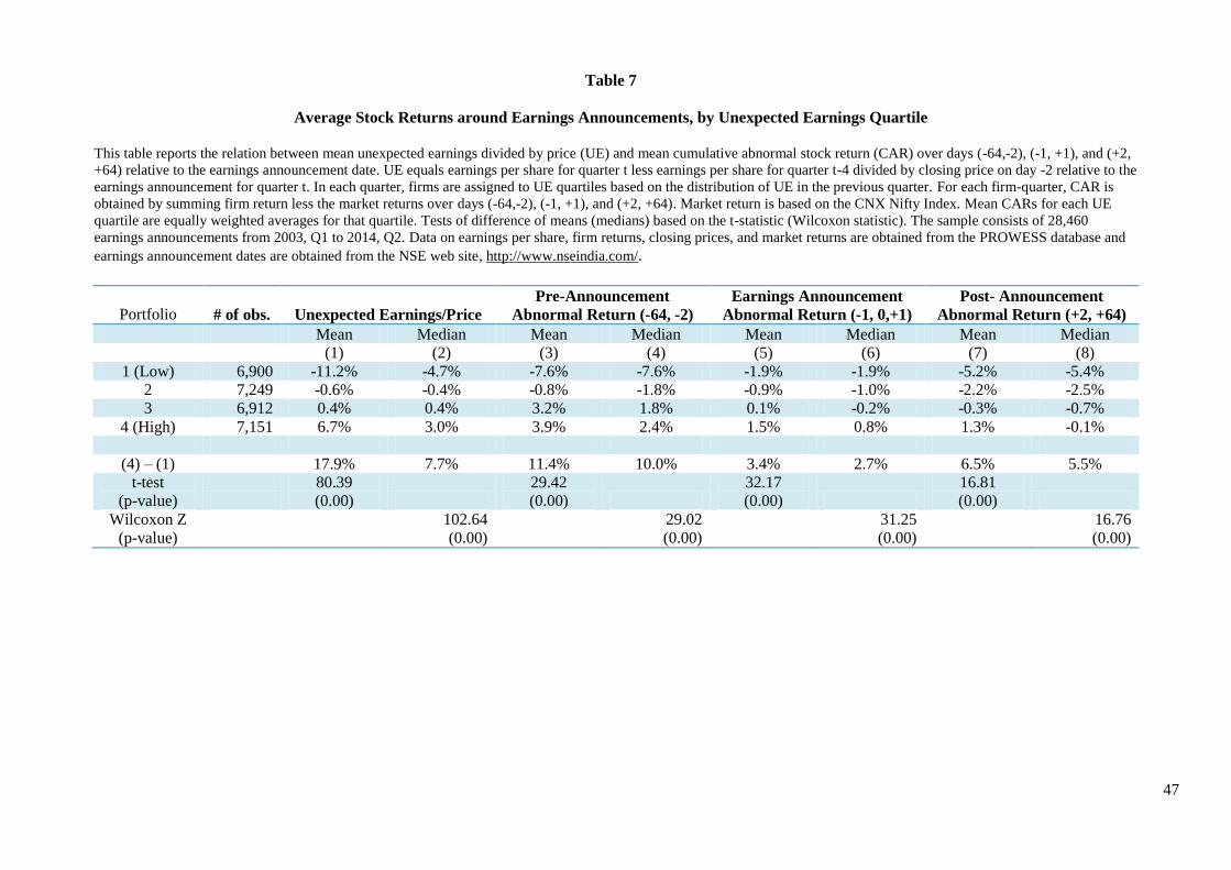
47
Table 7
Average Stock Returns around Earnings Announcements, by Unexpected Earnings Quartile
This table reports the relation between mean unexpected earnings divided by price (UE) and mean cumulative abnormal stock return (CAR) over days (-64,-2), (-1, +1), and (+2,
+64) relative to the earnings announcement date. UE equals earnings per share for quarter t less earnings per share for quarter t-4 divided by closing price on day -2 relative to the
earnings announcement for quarter t. In each quarter, firms are assigned to UE quartiles based on the distribution of UE in the previous quarter. For each firm-quarter, CAR is
obtained by summing firm return less the market returns over days (-64,-2), (-1, +1), and (+2, +64). Market return is based on the CNX Nifty Index. Mean CARs for each UE
quartile are equally weighted averages for that quartile. Tests of difference of means (medians) based on the t-statistic (Wilcoxon statistic). The sample consists of 28,460
earnings announcements from 2003, Q1 to 2014, Q2. Data on earnings per share, firm returns, closing prices, and market returns are obtained from the PROWESS database and
earnings announcement dates are obtained from the NSE web site, http://www.nseindia.com/.
Portfolio # of obs. Unexpected Earnings/Price
Pre-Announcement
Abnormal Return (-64, -2)
Earnings Announcement
Abnormal Return (-1, 0,+1)
Post- Announcement
Abnormal Return (+2, +64)
Mean Median Mean Median Mean Median Mean Median
(1) (2) (3) (4) (5) (6) (7) (8)
1 (Low) 6,900 -11.2% -4.7% -7.6% -7.6% -1.9% -1.9% -5.2% -5.4%
2 7,249 -0.6% -0.4% -0.8% -1.8% -0.9% -1.0% -2.2% -2.5%
3 6,912 0.4% 0.4% 3.2% 1.8% 0.1% -0.2% -0.3% -0.7%
4 (High) 7,151 6.7% 3.0% 3.9% 2.4% 1.5% 0.8% 1.3% -0.1%
(4) – (1) 17.9% 7.7% 11.4% 10.0% 3.4% 2.7% 6.5% 5.5%
t-test
(p-value)
80.39
(0.00)
29.42
(0.00)
32.17
(0.00)
16.81
(0.00)
Wilcoxon Z
(p-value)
102.64
(0.00)
29.02
(0.00)
31.25
(0.00)
16.76
(0.00)
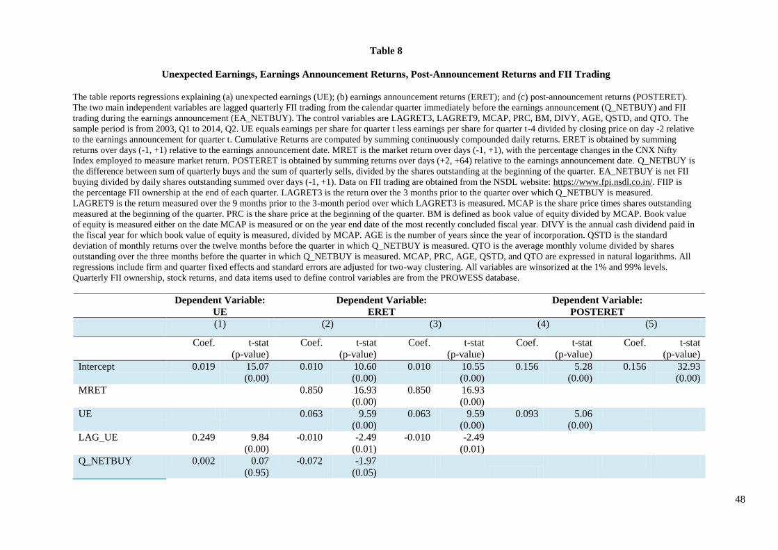
48
Table 8
Unexpected Earnings, Earnings Announcement Returns, Post-Announcement Returns and FII Trading
The table reports regressions explaining (a) unexpected earnings (UE); (b) earnings announcement returns (ERET); and (c) post-announcement returns (POSTERET).
The two main independent variables are lagged quarterly FII trading from the calendar quarter immediately before the earnings announcement (Q_NETBUY) and FII
trading during the earnings announcement (EA_NETBUY). The control variables are LAGRET3, LAGRET9, MCAP, PRC, BM, DIVY, AGE, QSTD, and QTO. The
sample period is from 2003, Q1 to 2014, Q2. UE equals earnings per share for quarter t less earnings per share for quarter t-4 divided by closing price on day -2 relative
to the earnings announcement for quarter t. Cumulative Returns are computed by summing continuously compounded daily returns. ERET is obtained by summing
returns over days (-1, +1) relative to the earnings announcement date. MRET is the market return over days (-1, +1), with the percentage changes in the CNX Nifty
Index employed to measure market return. POSTERET is obtained by summing returns over days (+2, +64) relative to the earnings announcement date. Q_NETBUY is
the difference between sum of quarterly buys and the sum of quarterly sells, divided by the shares outstanding at the beginning of the quarter. EA_NETBUY is net FII
buying divided by daily shares outstanding summed over days (-1, +1). Data on FII trading are obtained from the NSDL website: https://www.fpi.nsdl.co.in/. FIIP is
the percentage FII ownership at the end of each quarter. LAGRET3 is the return over the 3 months prior to the quarter over which Q_NETBUY is measured.
LAGRET9 is the return measured over the 9 months prior to the 3-month period over which LAGRET3 is measured. MCAP is the share price times shares outstanding
measured at the beginning of the quarter. PRC is the share price at the beginning of the quarter. BM is defined as book value of equity divided by MCAP. Book value
of equity is measured either on the date MCAP is measured or on the year end date of the most recently concluded fiscal year. DIVY is the annual cash dividend paid in
the fiscal year for which book value of equity is measured, divided by MCAP. AGE is the number of years since the year of incorporation. QSTD is the standard
deviation of monthly returns over the twelve months before the quarter in which Q_NETBUY is measured. QTO is the average monthly volume divided by shares
outstanding over the three months before the quarter in which Q_NETBUY is measured. MCAP, PRC, AGE, QSTD, and QTO are expressed in natural logarithms. All
regressions include firm and quarter fixed effects and standard errors are adjusted for two-way clustering. All variables are winsorized at the 1% and 99% levels.
Quarterly FII ownership, stock returns, and data items used to define control variables are from the PROWESS database.
Dependent Variable:
UE
Dependent Variable:
ERET
Dependent Variable:
POSTERET
(1) (2) (3) (4) (5)
Coef. t-stat
(p-value)
Coef. t-stat
(p-value)
Coef. t-stat
(p-value)
Coef. t-stat
(p-value)
Coef. t-stat
(p-value)
Intercept 0.019 15.07
(0.00)
0.010 10.60
(0.00)
0.010 10.55
(0.00)
0.156 5.28
(0.00)
0.156 32.93
(0.00)
MRET 0.850 16.93
(0.00)
0.850 16.93
(0.00)
UE 0.063 9.59
(0.00)
0.063 9.59
(0.00)
0.093 5.06
(0.00)
LAG_UE 0.249 9.84
(0.00)
-0.010 -2.49
(0.01)
-0.010 -2.49
(0.01)
Q_NETBUY 0.002 0.07
(0.95)
-0.072 -1.97
(0.05)
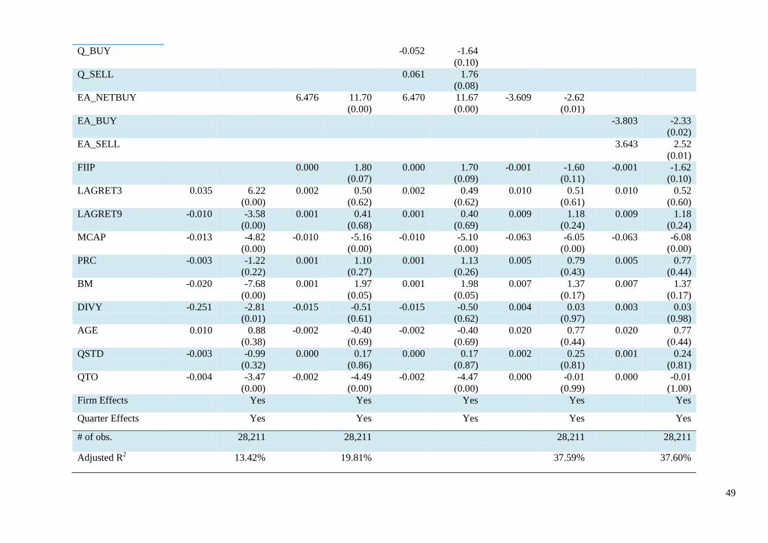
49
Q_BUY -0.052 -1.64
(0.10)
Q_SELL 0.061 1.76
(0.08)
EA_NETBUY 6.476 11.70
(0.00)
6.470 11.67
(0.00)
-3.609 -2.62
(0.01)
EA_BUY -3.803 -2.33
(0.02)
EA_SELL 3.643 2.52
(0.01)
FIIP 0.000 1.80
(0.07)
0.000 1.70
(0.09)
-0.001 -1.60
(0.11)
-0.001 -1.62
(0.10)
LAGRET3 0.035 6.22
(0.00)
0.002 0.50
(0.62)
0.002 0.49
(0.62)
0.010 0.51
(0.61)
0.010 0.52
(0.60)
LAGRET9 -0.010 -3.58
(0.00)
0.001 0.41
(0.68)
0.001 0.40
(0.69)
0.009 1.18
(0.24)
0.009 1.18
(0.24)
MCAP -0.013 -4.82
(0.00)
-0.010 -5.16
(0.00)
-0.010 -5.10
(0.00)
-0.063 -6.05
(0.00)
-0.063 -6.08
(0.00)
PRC -0.003 -1.22
(0.22)
0.001 1.10
(0.27)
0.001 1.13
(0.26)
0.005 0.79
(0.43)
0.005 0.77
(0.44)
BM -0.020 -7.68
(0.00)
0.001 1.97
(0.05)
0.001 1.98
(0.05)
0.007 1.37
(0.17)
0.007 1.37
(0.17)
DIVY -0.251 -2.81
(0.01)
-0.015 -0.51
(0.61)
-0.015 -0.50
(0.62)
0.004 0.03
(0.97)
0.003 0.03
(0.98)
AGE 0.010 0.88
(0.38)
-0.002 -0.40
(0.69)
-0.002 -0.40
(0.69)
0.020 0.77
(0.44)
0.020 0.77
(0.44)
QSTD -0.003 -0.99
(0.32)
0.000 0.17
(0.86)
0.000 0.17
(0.87)
0.002 0.25
(0.81)
0.001 0.24
(0.81)
QTO -0.004 -3.47
(0.00)
-0.002 -4.49
(0.00)
-0.002 -4.47
(0.00)
0.000 -0.01
(0.99)
0.000 -0.01
(1.00)
Firm Effects Yes Yes Yes Yes Yes
Quarter Effects Yes Yes Yes Yes Yes
# of obs. 28,211 28,211 28,211 28,211
Adjusted R2 13.42% 19.81% 37.59% 37.60%
Recommended

![On the Returns of Trend-Following Trading Strategies · success rate in relation to a fair game. ... Paper [II] measures the returns of a popular day trading strategy, ... returns](https://img.pdfslide.net/doc/110x75/5b3b95ec7f8b9a895a8c9502/on-the-returns-of-trend-following-trading-success-rate-in-relation-to-a-fair.jpg)