Periods, Galois theory and particle physics
Francis BrownAll Souls College, Oxford
Gergen Lectures,21st-24th March 2016
1 / 29
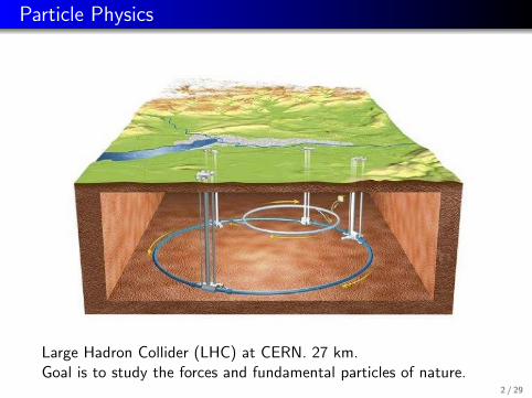
Particle Physics
Large Hadron Collider (LHC) at CERN. 27 km.Goal is to study the forces and fundamental particles of nature.
2 / 29
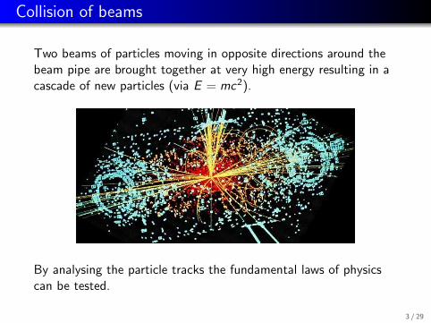
Collision of beams
Two beams of particles moving in opposite directions around thebeam pipe are brought together at very high energy resulting in acascade of new particles (via E = mc2).
By analysing the particle tracks the fundamental laws of physicscan be tested.
3 / 29
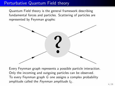
Perturbative Quantum Field theory
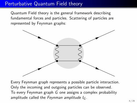
Quantum Field theory is the general framework describingfundamental forces and particles. Scattering of particles arerepresented by Feynman graphs:
?Every Feynman graph represents a possible particle interaction.Only the incoming and outgoing particles can be observed.To every Feynman graph G one assigns a complex probabilityamplitude called the Feynman amplitude IG .
4 / 29

Perturbative Quantum Field theory
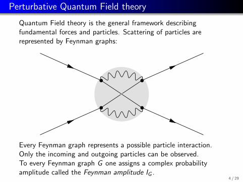
Quantum Field theory is the general framework describingfundamental forces and particles. Scattering of particles arerepresented by Feynman graphs:
Every Feynman graph represents a possible particle interaction.Only the incoming and outgoing particles can be observed.To every Feynman graph G one assigns a complex probabilityamplitude called the Feynman amplitude IG .
4 / 29

Perturbative Quantum Field theory
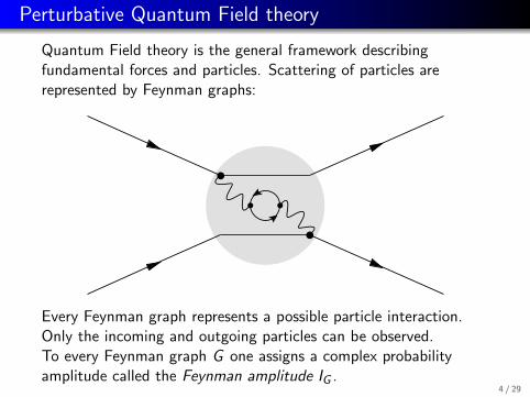
Quantum Field theory is the general framework describingfundamental forces and particles. Scattering of particles arerepresented by Feynman graphs:
Every Feynman graph represents a possible particle interaction.Only the incoming and outgoing particles can be observed.To every Feynman graph G one assigns a complex probabilityamplitude called the Feynman amplitude IG .
4 / 29
Perturbative Quantum Field theory
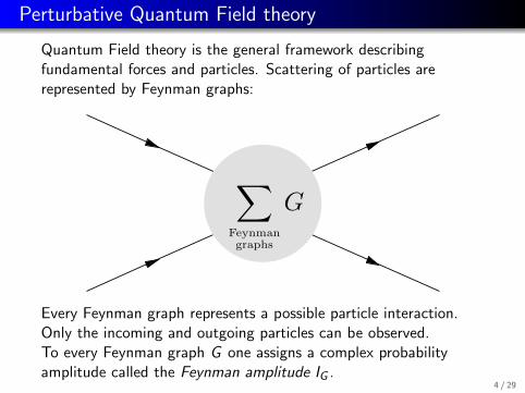
Quantum Field theory is the general framework describingfundamental forces and particles. Scattering of particles arerepresented by Feynman graphs:
∑
Feynmangraphs
G
Every Feynman graph represents a possible particle interaction.Only the incoming and outgoing particles can be observed.To every Feynman graph G one assigns a complex probabilityamplitude called the Feynman amplitude IG .
4 / 29
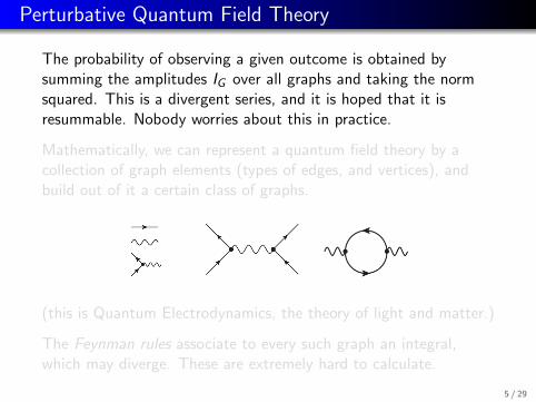
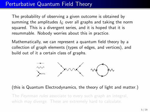
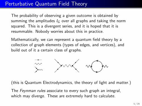
Perturbative Quantum Field Theory
The probability of observing a given outcome is obtained bysumming the amplitudes IG over all graphs and taking the normsquared. This is a divergent series, and it is hoped that it isresummable. Nobody worries about this in practice.
Mathematically, we can represent a quantum field theory by acollection of graph elements (types of edges, and vertices), andbuild out of it a certain class of graphs.
(this is Quantum Electrodynamics, the theory of light and matter.)
The Feynman rules associate to every such graph an integral,which may diverge. These are extremely hard to calculate.
5 / 29
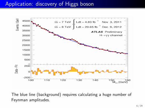
Application: discovery of Higgs boson
The blue line (background) requires calculating a huge number ofFeynman amplitudes.
6 / 29
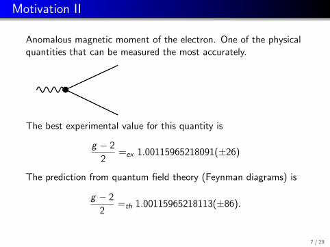
Motivation II
Anomalous magnetic moment of the electron. One of the physicalquantities that can be measured the most accurately.
The best experimental value for this quantity is
g − 2
2=ex 1.00115965218091(±26)
The prediction from quantum field theory (Feynman diagrams) is
g − 2
2=th 1.00115965218113(±86).
7 / 29

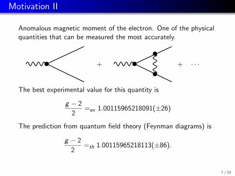
Motivation II
Anomalous magnetic moment of the electron. One of the physicalquantities that can be measured the most accurately.
+ + · · ·
The best experimental value for this quantity is
g − 2
2=ex 1.00115965218091(±26)
The prediction from quantum field theory (Feynman diagrams) is
g − 2
2=th 1.00115965218113(±86).
7 / 29
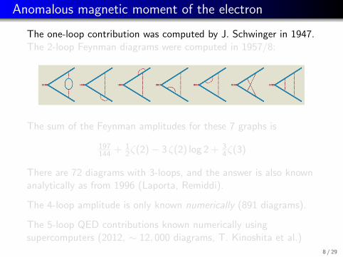
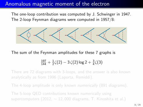
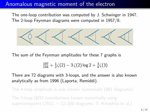
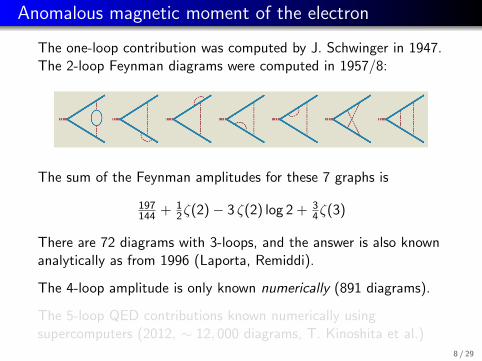
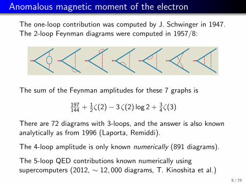
Anomalous magnetic moment of the electron
The one-loop contribution was computed by J. Schwinger in 1947.The 2-loop Feynman diagrams were computed in 1957/8:
The sum of the Feynman amplitudes for these 7 graphs is
197144 + 1
2ζ(2)− 3 ζ(2) log 2 + 34ζ(3)
There are 72 diagrams with 3-loops, and the answer is also knownanalytically as from 1996 (Laporta, Remiddi).
The 4-loop amplitude is only known numerically (891 diagrams).
The 5-loop QED contributions known numerically usingsupercomputers (2012, ∼ 12, 000 diagrams, T. Kinoshita et al.)
8 / 29
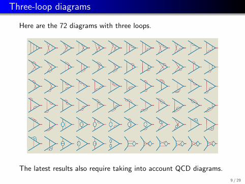
Three-loop diagrams
Here are the 72 diagrams with three loops.
The latest results also require taking into account QCD diagrams.
9 / 29
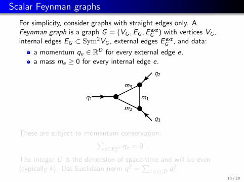
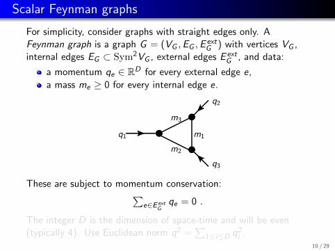
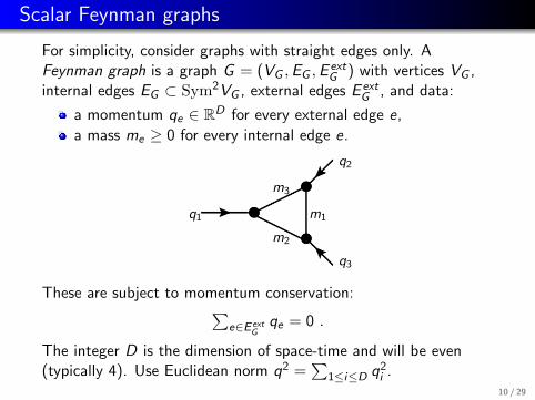
Scalar Feynman graphs
For simplicity, consider graphs with straight edges only. AFeynman graph is a graph G = (VG ,EG ,E
extG ) with vertices VG ,
internal edges EG ⊂ Sym2VG , external edges E extG , and data:
a momentum qe ∈ RD for every external edge e,
a mass me ≥ 0 for every internal edge e.
q1
q2
q3
m1
m2
m3
These are subject to momentum conservation:∑e∈E ext
Gqe = 0 .
The integer D is the dimension of space-time and will be even(typically 4). Use Euclidean norm q2 =
∑1≤i≤D q2
i .10 / 29
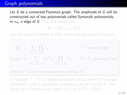
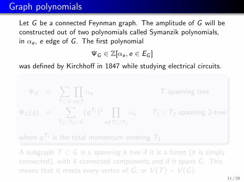
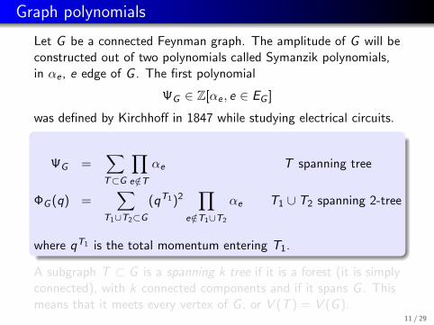
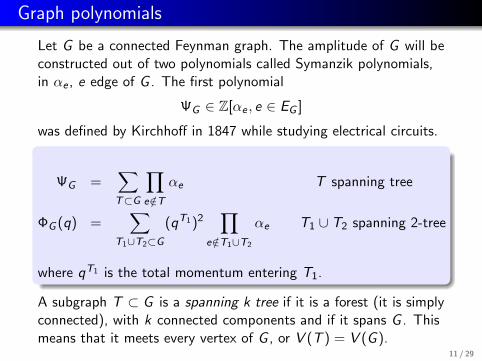
Graph polynomials
Let G be a connected Feynman graph. The amplitude of G will beconstructed out of two polynomials called Symanzik polynomials,in αe , e edge of G . The first polynomial
ΨG ∈ Z[αe , e ∈ EG ]
was defined by Kirchhoff in 1847 while studying electrical circuits.
ΨG =∑T⊂G
∏e /∈T
αe T spanning tree
ΦG (q) =∑
T1∪T2⊂G
(qT1)2∏
e /∈T1∪T2
αe T1 ∪ T2 spanning 2-tree
where qT1 is the total momentum entering T1.
A subgraph T ⊂ G is a spanning k tree if it is a forest (it is simplyconnected), with k connected components and if it spans G . Thismeans that it meets every vertex of G , or V (T ) = V (G ).
11 / 29
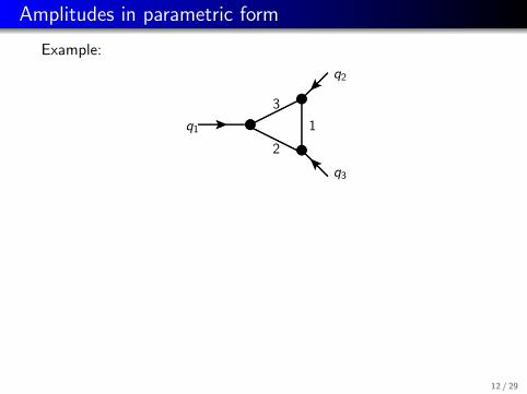
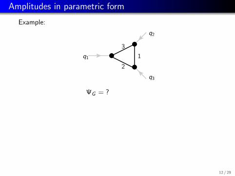
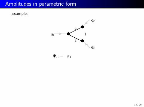
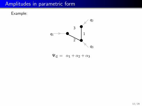
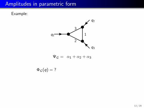
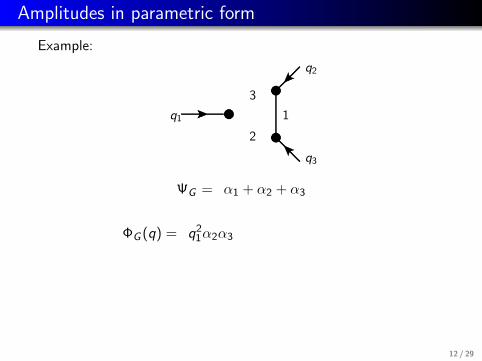
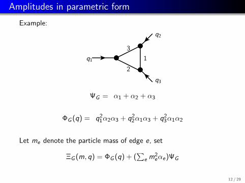
Amplitudes in parametric form
Example:
q1 1
q2
2
q3
3
ΨG = ?α1 + α2 + α3
ΦG (q) = ?q21α2α3 + q2
2α1α3 + q23α1α2
Let me denote the particle mass of edge e, set
ΞG (m, q) = ΦG (q) + (∑
e m2eαe)ΨG
12 / 29
Amplitudes in parametric form
Example:
q1 1
q2
2
q3
3
ΨG = ?
α1 + α2 + α3
ΦG (q) = ?q21α2α3 + q2
2α1α3 + q23α1α2
Let me denote the particle mass of edge e, set
ΞG (m, q) = ΦG (q) + (∑
e m2eαe)ΨG
12 / 29
Amplitudes in parametric form
Example:
q1 1
q2
2
q3
3
ΨG =
?
α1
+ α2 + α3
ΦG (q) = ?q21α2α3 + q2
2α1α3 + q23α1α2
Let me denote the particle mass of edge e, set
ΞG (m, q) = ΦG (q) + (∑
e m2eαe)ΨG
12 / 29

Amplitudes in parametric form
Example:
q1 1
q2
2
q3
3
ΨG =
?
α1 + α2
+ α3
ΦG (q) = ?q21α2α3 + q2
2α1α3 + q23α1α2
Let me denote the particle mass of edge e, set
ΞG (m, q) = ΦG (q) + (∑
e m2eαe)ΨG
12 / 29
Amplitudes in parametric form
Example:
q1 1
q2
2
q3
3
ΨG =
?
α1 + α2 + α3
ΦG (q) = ?q21α2α3 + q2
2α1α3 + q23α1α2
Let me denote the particle mass of edge e, set
ΞG (m, q) = ΦG (q) + (∑
e m2eαe)ΨG
12 / 29
Amplitudes in parametric form
Example:
q1 1
q2
2
q3
3
ΨG =
?
α1 + α2 + α3
ΦG (q) = ?
q21α2α3 + q2
2α1α3 + q23α1α2
Let me denote the particle mass of edge e, set
ΞG (m, q) = ΦG (q) + (∑
e m2eαe)ΨG
12 / 29
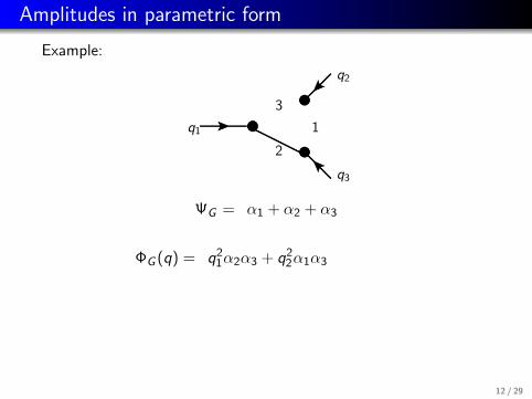
Amplitudes in parametric form
Example:
q1 1
q2
2
q3
3
ΨG =
?
α1 + α2 + α3
ΦG (q) =
?
q21α2α3
+ q22α1α3 + q2
3α1α2
Let me denote the particle mass of edge e, set
ΞG (m, q) = ΦG (q) + (∑
e m2eαe)ΨG
12 / 29
Amplitudes in parametric form
Example:
q1 1
q2
2
q3
3
ΨG =
?
α1 + α2 + α3
ΦG (q) =
?
q21α2α3 + q2
2α1α3
+ q23α1α2
Let me denote the particle mass of edge e, set
ΞG (m, q) = ΦG (q) + (∑
e m2eαe)ΨG
12 / 29
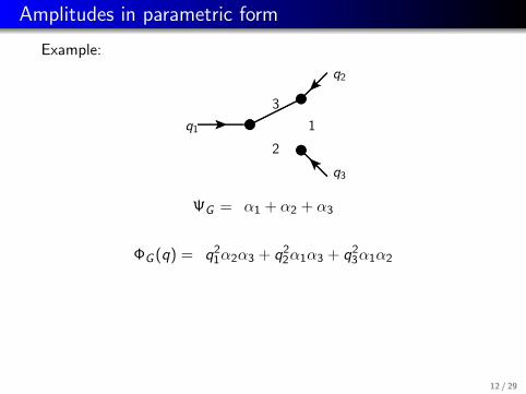
Amplitudes in parametric form
Example:
q1 1
q2
2
q3
3
ΨG =
?
α1 + α2 + α3
ΦG (q) =
?
q21α2α3 + q2
2α1α3 + q23α1α2
Let me denote the particle mass of edge e, set
ΞG (m, q) = ΦG (q) + (∑
e m2eαe)ΨG
12 / 29
Amplitudes in parametric form
Example:
q1 1
q2
2
q3
3
ΨG =
?
α1 + α2 + α3
ΦG (q) =
?
q21α2α3 + q2
2α1α3 + q23α1α2
Let me denote the particle mass of edge e, set
ΞG (m, q) = ΦG (q) + (∑
e m2eαe)ΨG
12 / 29
Amplitudes in parametric form
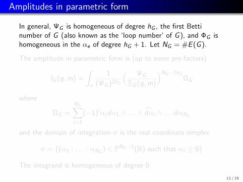
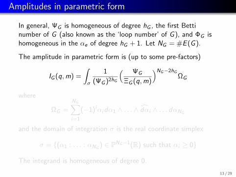
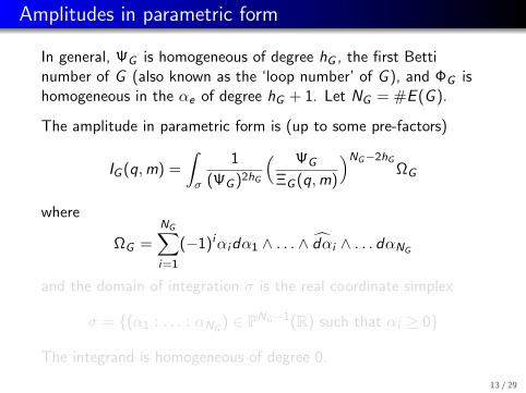
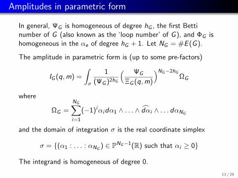
In general, ΨG is homogeneous of degree hG , the first Bettinumber of G (also known as the ‘loop number’ of G ), and ΦG ishomogeneous in the αe of degree hG + 1. Let NG = #E (G ).
The amplitude in parametric form is (up to some pre-factors)
IG (q,m) =
∫σ
1
(ΨG )2hG
( ΨG
ΞG (q,m)
)NG−2hG
ΩG
where
ΩG =
NG∑i=1
(−1)iαidα1 ∧ . . . ∧ dαi ∧ . . . dαNG
and the domain of integration σ is the real coordinate simplex
σ = (α1 : . . . : αNG) ∈ PNG−1(R) such that αi ≥ 0
The integrand is homogeneous of degree 0.
13 / 29
Amplitudes in parametric form
In general, ΨG is homogeneous of degree hG , the first Bettinumber of G (also known as the ‘loop number’ of G ), and ΦG ishomogeneous in the αe of degree hG + 1. Let NG = #E (G ).
The amplitude in parametric form is (up to some pre-factors)
IG (q,m) =
∫σ
1
(ΨG )2hG
( ΨG
ΞG (q,m)
)NG−2hG
ΩG
where
ΩG =
NG∑i=1
(−1)iαidα1 ∧ . . . ∧ dαi ∧ . . . dαNG
and the domain of integration σ is the real coordinate simplex
σ = (α1 : . . . : αNG) ∈ PNG−1(R) such that αi ≥ 0
The integrand is homogeneous of degree 0.
13 / 29
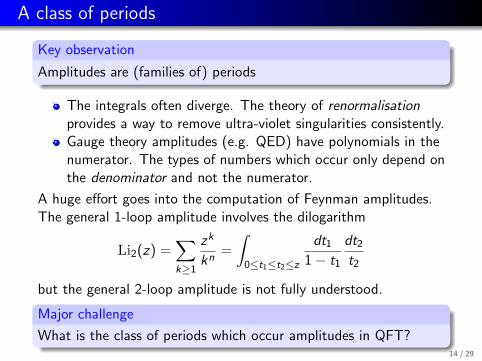
A class of periods
Key observation
Amplitudes are (families of) periods
The integrals often diverge. The theory of renormalisationprovides a way to remove ultra-violet singularities consistently.Gauge theory amplitudes (e.g. QED) have polynomials in thenumerator. The types of numbers which occur only depend onthe denominator and not the numerator.
A huge effort goes into the computation of Feynman amplitudes.The general 1-loop amplitude involves the dilogarithm
Li2(z) =∑k≥1
zk
kn=
∫0≤t1≤t2≤z
dt1
1− t1
dt2
t2
but the general 2-loop amplitude is not fully understood.
Major challenge
What is the class of periods which occur amplitudes in QFT?14 / 29
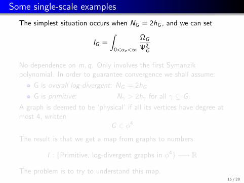
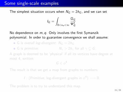
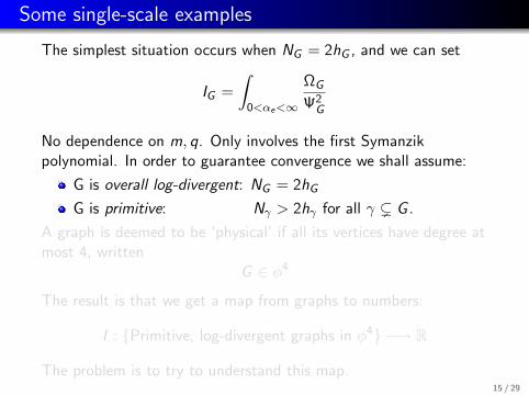
Some single-scale examples
The simplest situation occurs when NG = 2hG , and we can set
IG =
∫0<αe<∞
ΩG
Ψ2G
No dependence on m, q. Only involves the first Symanzikpolynomial. In order to guarantee convergence we shall assume:
G is overall log-divergent: NG = 2hG
G is primitive: Nγ > 2hγ for all γ ( G .
A graph is deemed to be ‘physical’ if all its vertices have degree atmost 4, written
G ∈ φ4
The result is that we get a map from graphs to numbers:
I : Primitive, log-divergent graphs in φ4 −→ R
The problem is to try to understand this map.15 / 29
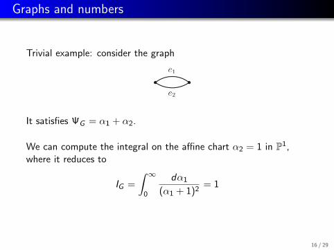
Graphs and numbers
Trivial example: consider the graph
It satisfies ΨG = α1 + α2.
We can compute the integral on the affine chart α2 = 1 in P1,where it reduces to
IG =
∫ ∞0
dα1
(α1 + 1)2= 1
16 / 29
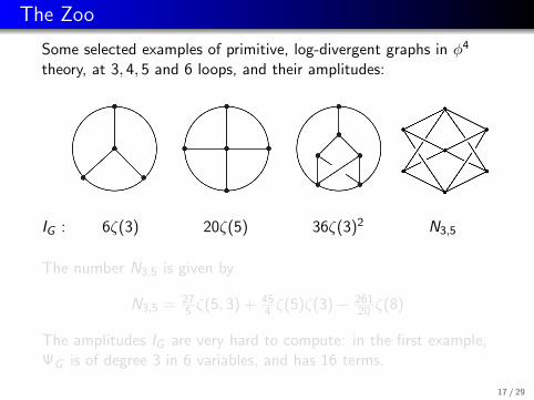
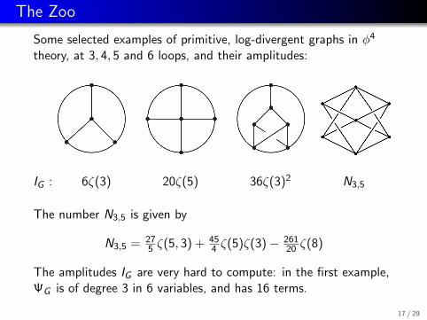
The Zoo
Some selected examples of primitive, log-divergent graphs in φ4
theory, at 3, 4, 5 and 6 loops, and their amplitudes:
IG : 6ζ(3) 20ζ(5) 36ζ(3)2 N3,5
The number N3,5 is given by
N3,5 = 275 ζ(5, 3) + 45
4 ζ(5)ζ(3)− 26120 ζ(8)
The amplitudes IG are very hard to compute: in the first example,ΨG is of degree 3 in 6 variables, and has 16 terms.
17 / 29
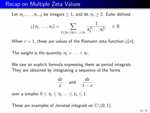
Recap on Multiple Zeta Values
Let n1, . . . , nr−1 be integers ≥ 1, and let nr ≥ 2. Euler defined
ζ(n1, . . . , nr ) =∑
1≤k1<k2<...<kr
1
kn11 . . . knr
r∈ R
When r = 1, these are values of the Riemann zeta function ζ(n).
The weight is the quantity n1 + . . .+ nr .
We saw an explicit formula expressing them as period integrals.They are obtained by integrating a sequence of the forms
dz
zand
dz
1− z
over a simplex 0 ≤ t1 ≤ t2 . . . ≤ tn ≤ 1.
These are examples of iterated integrals on C\0, 1.18 / 29
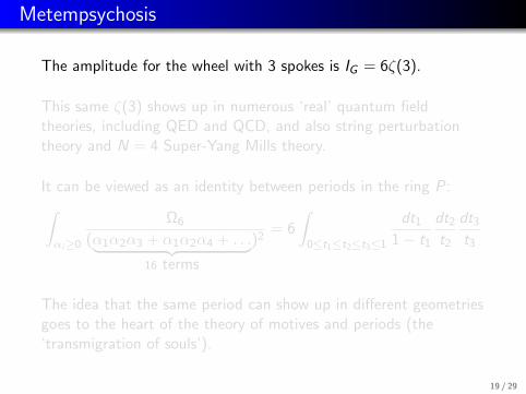
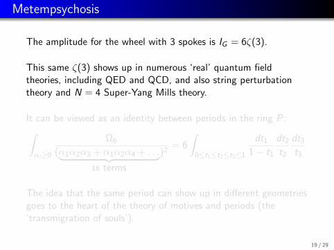
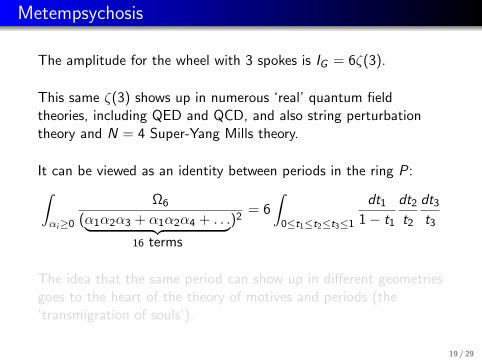
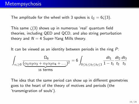
Metempsychosis
The amplitude for the wheel with 3 spokes is IG = 6ζ(3).
This same ζ(3) shows up in numerous ‘real’ quantum fieldtheories, including QED and QCD, and also string perturbationtheory and N = 4 Super-Yang Mills theory.
It can be viewed as an identity between periods in the ring P:∫αi≥0
Ω6
(α1α2α3 + α1α2α4 + . . .︸ ︷︷ ︸16 terms
)2= 6
∫0≤t1≤t2≤t3≤1
dt1
1− t1
dt2
t2
dt3
t3
The idea that the same period can show up in different geometriesgoes to the heart of the theory of motives and periods (the‘transmigration of souls’).
19 / 29
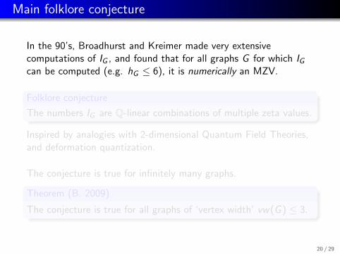
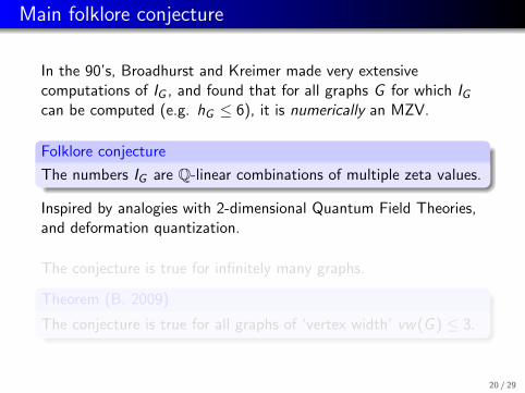
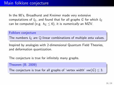
Main folklore conjecture
In the 90’s, Broadhurst and Kreimer made very extensivecomputations of IG , and found that for all graphs G for which IGcan be computed (e.g. hG ≤ 6), it is numerically an MZV.
Folklore conjecture
The numbers IG are Q-linear combinations of multiple zeta values.
Inspired by analogies with 2-dimensional Quantum Field Theories,and deformation quantization.
The conjecture is true for infinitely many graphs.
Theorem (B. 2009)
The conjecture is true for all graphs of ‘vertex width’ vw(G ) ≤ 3.
20 / 29
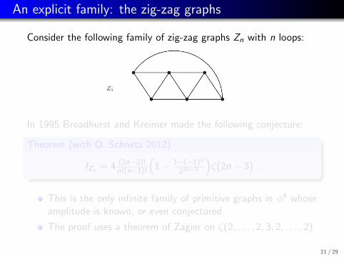
An explicit family: the zig-zag graphs
Consider the following family of zig-zag graphs Zn with n loops:
In 1995 Broadhurst and Kreimer made the following conjecture:
Theorem (with O. Schnetz 2012)
IZn = 4 (2n−2)!n!(n−1)!
(1− 1−(−1)n
22n−3
)ζ(2n − 3) .
This is the only infinite family of primitive graphs in φ4 whoseamplitude is known, or even conjectured.
The proof uses a theorem of Zagier on ζ(2, . . . , 2, 3, 2, . . . , 2)
21 / 29
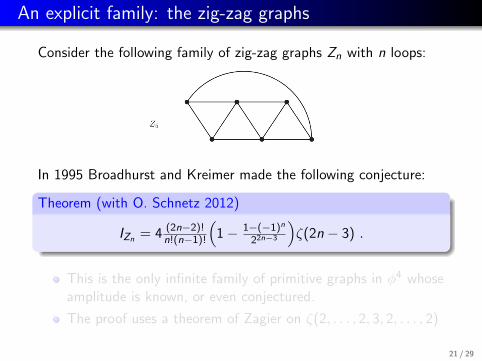
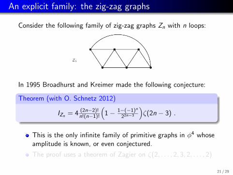
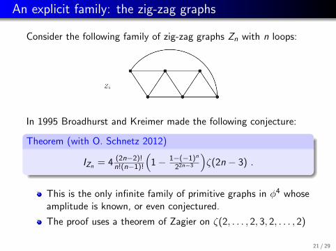
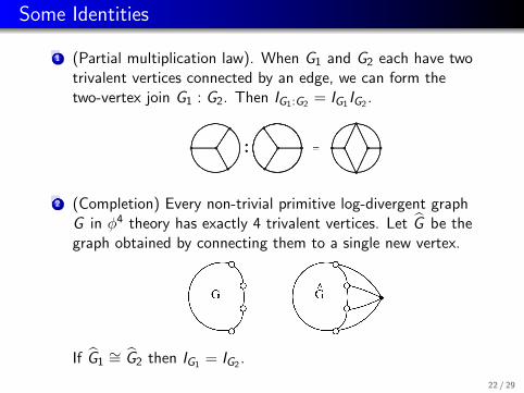
Some Identities
1 (Partial multiplication law). When G1 and G2 each have twotrivalent vertices connected by an edge, we can form thetwo-vertex join G1 : G2. Then IG1:G2 = IG1 IG2 .
2 (Completion) Every non-trivial primitive log-divergent graphG in φ4 theory has exactly 4 trivalent vertices. Let G be thegraph obtained by connecting them to a single new vertex.
If G1∼= G2 then IG1 = IG2 .
22 / 29
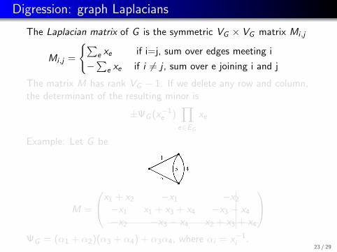
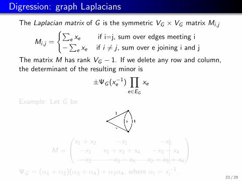
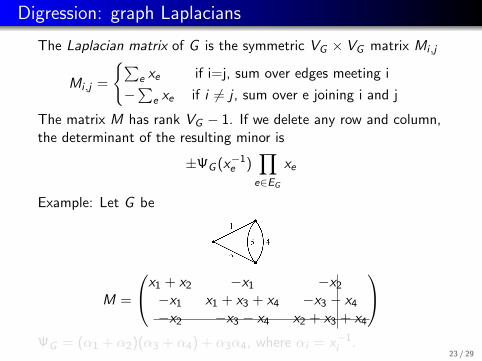
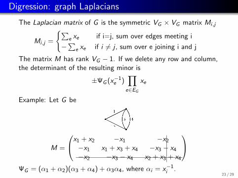
Digression: graph Laplacians
The Laplacian matrix of G is the symmetric VG × VG matrix Mi ,j
Mi ,j =
∑e xe if i=j, sum over edges meeting i
−∑
e xe if i 6= j , sum over e joining i and j
The matrix M has rank VG − 1. If we delete any row and column,the determinant of the resulting minor is
±ΨG (x−1e )
∏e∈EG
xe
Example: Let G be
M =
x1 + x2 −x1 −x2
−x1 x1 + x3 + x4 −x3 − x4
−x2 −x3 − x4 x2 + x3 + x4
ΨG = (α1 + α2)(α3 + α4) + α3α4, where αi = x−1
i .23 / 29
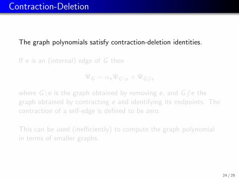
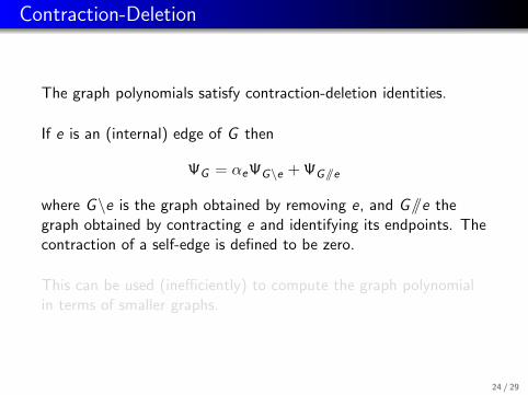
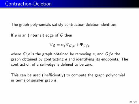
Contraction-Deletion
The graph polynomials satisfy contraction-deletion identities.
If e is an (internal) edge of G then
ΨG = αeΨG\e + ΨG//e
where G\e is the graph obtained by removing e, and G//e thegraph obtained by contracting e and identifying its endpoints. Thecontraction of a self-edge is defined to be zero.
This can be used (inefficiently) to compute the graph polynomialin terms of smaller graphs.
24 / 29
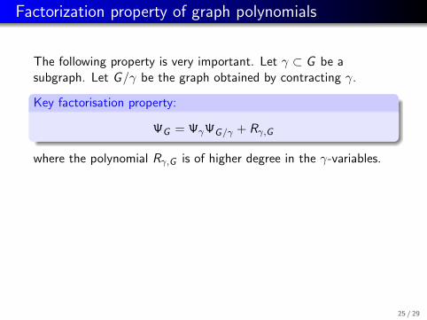
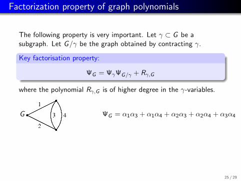
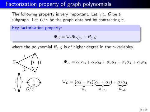
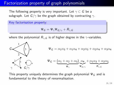
Factorization property of graph polynomials
The following property is very important. Let γ ⊂ G be asubgraph. Let G/γ be the graph obtained by contracting γ.
Key factorisation property:
ΨG = ΨγΨG/γ + Rγ,G
where the polynomial Rγ,G is of higher degree in the γ-variables.
G ΨG = α1α3 + α1α4 + α2α3 + α2α4 + α3α4
This property uniquely determines the graph polynomial ΨG and isfundamental to the theory of renormalisation.
25 / 29
Factorization property of graph polynomials
The following property is very important. Let γ ⊂ G be asubgraph. Let G/γ be the graph obtained by contracting γ.
Key factorisation property:
ΨG = ΨγΨG/γ + Rγ,G
where the polynomial Rγ,G is of higher degree in the γ-variables.
G ΨG = α1α3 + α1α4 + α2α3 + α2α4 + α3α4
γ G/γ
1
2
3 4 ΨG = (α3 + α4)︸ ︷︷ ︸Ψγ
(α1 + α2︸ ︷︷ ︸ΨG/γ
) + α3α4︸ ︷︷ ︸Rγ,G
This property uniquely determines the graph polynomial ΨG and isfundamental to the theory of renormalisation.
25 / 29
Factorization property of graph polynomials
The following property is very important. Let γ ⊂ G be asubgraph. Let G/γ be the graph obtained by contracting γ.
Key factorisation property:
ΨG = ΨγΨG/γ + Rγ,G
where the polynomial Rγ,G is of higher degree in the γ-variables.
G ΨG = α1α3 + α1α4 + α2α3 + α2α4 + α3α4
γ G/γ
43
1
2
ΨG = (α1 + α2 + α3)︸ ︷︷ ︸Ψγ
α4︸︷︷︸ΨG/γ
+α1α3 + α2α3︸ ︷︷ ︸Rγ,G
This property uniquely determines the graph polynomial ΨG and isfundamental to the theory of renormalisation.
25 / 29
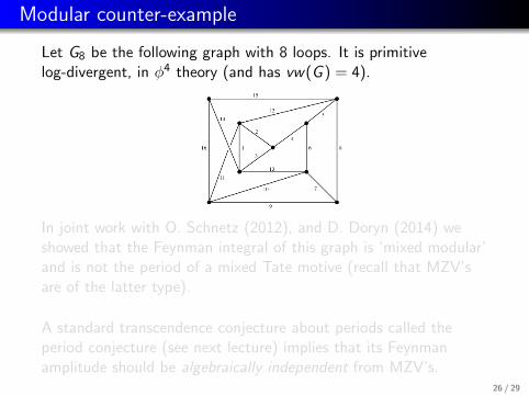
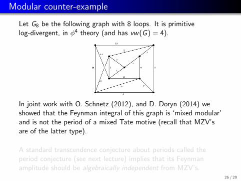
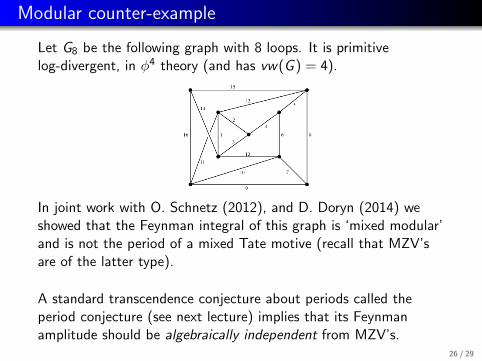
Modular counter-example
Let G8 be the following graph with 8 loops. It is primitivelog-divergent, in φ4 theory (and has vw(G ) = 4).
In joint work with O. Schnetz (2012), and D. Doryn (2014) weshowed that the Feynman integral of this graph is ‘mixed modular’and is not the period of a mixed Tate motive (recall that MZV’sare of the latter type).
A standard transcendence conjecture about periods called theperiod conjecture (see next lecture) implies that its Feynmanamplitude should be algebraically independent from MZV’s.
26 / 29
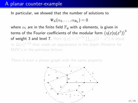
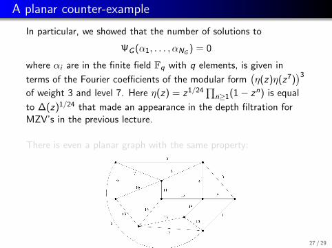
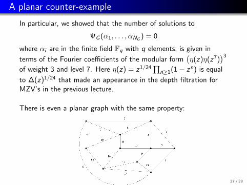
A planar counter-example
In particular, we showed that the number of solutions to
ΨG (α1, . . . , αNG) = 0
where αi are in the finite field Fq with q elements, is given in
terms of the Fourier coefficients of the modular form(η(z)η(z7)
)3
of weight 3 and level 7. Here η(z) = z1/24∏
n≥1(1− zn) is equal
to ∆(z)1/24 that made an appearance in the depth filtration forMZV’s in the previous lecture.
There is even a planar graph with the same property:
27 / 29
Conclusion
One of the simplest natural families of periods in mathematics arethe multiple zeta values. These are obtained by iterativelyintegrating the two differential forms
dz
zand
dz
1− z
over a single space: P1\0, 1,∞. We saw that they arise in manydifferent mathematical contexts.
On the other hand, the simplest family of periods in quantum fieldtheory are the amplitudes IG . The folklore conjecture, based on avast amount of evidence stated that
Amplitudes in φ4 ↔ Multiple Zeta values
In general we would like it to be true that
‘Quantities coming from QFT’ = ‘mathematically simple objects’28 / 29
Conclusion
But although φ4 amplitudes and MZV’s have a huge (infinite)overlap, they start to diverge radically at some point.
All versions of the folklore conjecture are true for small graphs butcompletely false in general. This suggests that there is no simpleanswer to describe amplitudes at all loop orders: the situation ismuch more complex, and interesting, than anyone imagined.
This begs a mathematical question: what is the next class ofperiods we should study after iterated integrals on
P1\0, 1,∞?
The fact that we saw modular forms appear in two quite differentcontexts: in the depth filtration for MZV’s and in the non-MZVcounter-examples in φ4 theory, gives a possible hint.
29 / 29
Recommended


![[copyright Taylor & Francis]vuir.vu.edu.au/30344/1/Transforming_communities_through_sport_C.… · Sarah Oxford Institute of Sport, Exercise and Active Living, Victoria University,](https://img.pdfslide.net/doc/110x75/60a74dc22659df26fe4063c6/copyright-taylor-francisvuirvueduau303441transformingcommunitiesthroughsportc.jpg)