Genesis of Hurricane Julia (2010) within an African Easterly Wave: SensitivityAnalyses of WRF-LETKF Ensemble Forecasts
STEFAN F. CECELSKI AND DA-LIN ZHANG
Department of Atmospheric and Oceanic Science, University of Maryland, College Park, College Park, Maryland
(Manuscript received 7 January 2014, in final form 21 April 2014)
ABSTRACT
In this study, the predictability of tropical cyclogenesis (TCG) is explored by conducting ensemble sensi-
tivity analyses on the TCG of Hurricane Julia (2010). Using empirical orthogonal functions (EOFs), the
dominant patterns of ensemble disagreements are revealed for various meteorological parameters such as
mean sea level pressure (MSLP) and upper-tropospheric temperature. Using the principal components of the
EOF patterns, ensemble sensitivities are generated to elucidate which mechanisms drive the parametric
ensemble differences.
The dominant pattern of MSLP ensemble spread is associated with the intensity of the pre–tropical de-
pression (pre-TD), explaining nearly half of the total variance at each respective time. Similar modes of
variance are found for the low-level absolute vorticity, though the patterns explain substantially less variance.
Additionally, the largest modes of variability associated with upper-level temperature anomalies closely
resemble the patterns of MSLP variance, suggesting interconnectedness between the two parameters. Sen-
sitivity analyses at both the pre-TD andTCG stages reveal that theMSLPdisturbance is strongly correlated to
upper-tropospheric temperature and, to a lesser degree, surface latent heat flux anomalies. Further sensitivity
analyses uncover a statistically significant correlation between upper-tropospheric temperature and con-
vective anomalies, consistent with the notion that deep convection is important for augmenting the upper-
tropospheric warmth during TCG. Overall, the ensemble forecast differences for the TCG of Julia are
strongly related to the processes responsible for MSLP falls and low-level cyclonic vorticity growth, including
the growth of upper-tropospheric warming and persistent deep convection.
1. Introduction
Although tropical cyclogenesis (TCG) has been amain
focus of numerous modeling studies and observational
campaigns in recent years, the formation of tropical de-
pressions (TDs) and their evolution into tropical storms
(TSs) remain poorly understood. The process by which a
nondeveloping tropical disturbance intensifies into a TS-
like system involves multiple scales of interactive pro-
cesses, ranging from cloud microphysics to meso-g- and
synoptic-scale motions. Theories to describe the forma-
tion of a low-level meso-b-scale vortex (LLV) within an
African easterly wave (AEW) have attempted to paint
a complete picture of TCGwithin an easterly wave in the
northern Atlantic and eastern Pacific basins. There still
are, however, many unanswered questions regarding the
dynamical and thermodynamical transitions taking place
during TCG because of the lack of high-resolution spatial
and temporal data.
Cloud-permitting models have been used to provide
novel insights into the development of some non-
observable features of TCG, such as convective bursts
(CBs) and meso-g-scale vortices (Cecelski and Zhang
2013, hereafter CZ). Additionally, numerous studies
have investigated the theories created to describe the
roles of the AEW during TCG in addition to the for-
mation of the LLV. TheAEWhas recently been thought
of as the parent to the LLV under the marsupial pouch
paradigm (Dunkerton et al. 2009; Wang et al. 2010;
Montgomery et al. 2010), with both observational
studies (Montgomery et al. 2012; Braun et al. 2013) and
high-resolution modeling studies having demonstrated
its usefulness. When the AEW is thought of in this
manner, the growth of the LLV is presumed to take
place from the bottom up, resulting from the formation
and aggregation of vortical hot towers (VHTs) and other
mesovortices (Hendricks et al. 2004; Montgomery et al.
Corresponding author address: Dr. Da-Lin Zhang, Department
of Atmospheric and Oceanic Science, University of Maryland,
College Park, College Park, MD 20742.
E-mail: [email protected]
3180 JOURNAL OF THE ATMOSPHER IC SC IENCES VOLUME 71
DOI: 10.1175/JAS-D-14-0006.1
� 2014 American Meteorological Society

2006; CZ). The existence of VHTs, mesovortices, and
their aggregation have been shown in observational and
modeling studies, supporting the notion that they are
the ‘‘building blocks of TCG’’ (Sippel et al. 2006; Houze
et al. 2009; CZ). More recently, upper-tropospheric
thermodynamic changes have been shown to induce
meso-a-scale mean sea level pressure (MSLP) falls
during TCG (Zhang and Zhu 2012; CZ), further sup-
plementing the marsupial pouch paradigm and the for-
mation of the LLV. TheMSLP falls aid the development
of the LLV via enhanced planetary boundary layer
(PBL) convergence near the AEW pouch center (CZ).
This warming aloft is not considered to be resultant from
balanced flow but instead by an imbalance of latent
heating due to the depositional growth of ice in the
upper troposphere (CZ).
A more innovative way to investigate the dynamics
and thermodynamics of TCG is through ensemble sim-
ulations, though its use has just begun. By perturbing the
initial conditions (ICs) of an individual model, a suite of
forecasts can be generated for the TCG of a particular
storm. Two notable studies have used a single model
ensemble to investigate TCG: Sippel and Zhang (2008)
and Cecelski et al. (2014, hereafter CZM). The former
used short-range fifth-generation Pennsylvania State
University–National Center for Atmospheric Research
Mesoscale Model (MM5) ensemble forecasts to in-
vestigate a nondeveloping disturbance in the Gulf of
Mexico and concluded that the presence of a moist
tropospheric column and high convective available po-
tential energy (CAPE) are the two most important ICs
for TCG. The higher CAPE and greater column mois-
ture content enables a faster spinup in some ensemble
members, which, in turn, undergo TCG faster. The latter
uses the Weather Research and Forecasting–local en-
semble transform Kalman filter coupled system (WRF-
LETKF; Hunt et al. 2007; Miyoshi and Kunii 2012) to
generate twenty 1-km-resolution ensemble forecasts for
the TCG of Hurricane Julia (2010). Their work showed
that the differences in TCG between the ensemble
members was related to convective initiation early in the
simulations in addition to the creation of a storm-scale
outflow and upper-tropospheric warming during TCG.
While CZM studied differences between developing
and nondeveloping members from the WRF-LETKF
ensemble forecasts, a statistical approach to making
inferences on the dynamics and thermodynamics (e.g.,
MSLP changes) of TCG can provide a more holistic view
of the ensemble forecasts. Sippel and Zhang (2008) em-
ployed a linear correlation analysis, following Hawblitzel
et al. (2007), to generate statistical sensitivities of MSLP
changes and isolated variables that are responsible dy-
namically for the changes. More recently, studies have
used ensemble sensitivity analyses (Chang et al. 2013;
Zheng et al. 2013; Gombos et al. 2012; Torn and Hakim
2008; Ancell and Hakim 2007) to examine how a partic-
ular forecast metric depends on ICs. Ensemble sensitivity
uses a linear correlation between a chosen forecastmetric
and selected meteorological parameters to generate
a statistical sensitivity of the forecast metric for previous
forecast times and the ICs. Instead of using just an in-
dividual ensemble member, the analysis is able to use all
ensemble members, yielding the ability to make infer-
ences about what meteorological parameters the whole
complement of ensemble forecasts are sensitive to. En-
semble sensitivity has been shown to be useful in short-
and medium-range forecasts for midlatitude applications
(Chang et al. 2013; Zheng et al. 2013), as well as TC track
forecasts (Gombos et al. 2012), even with the assumption
of linearity. The selection of a forecast metric has varied
across previous studies, ranging from selecting particular
cyclone parameters (e.g., MSLP) to the principal com-
ponents (PCs) of empirical orthogonal functions (EOFs),
whose use has produced promising results (Chang et al.
2013; Zheng et al. 2013; Gombos et al. 2012). Recently,
the use of ensemble sensitivity analyses via EOFs was
extended by Torn and Cook (2013) for two TCG cases
from the 2010 North Atlantic hurricane season. Their
results depicted that the forecasts of TCG were sensitive
to select, but different, parameters. The first storm inves-
tigated, Hurricane Danielle, was most sensitive to upper-
level divergence and deep-layer (e.g., 850–200 hPa)
vertical wind shear (VWS). In contrast, the second storm,
Hurricane Karl, was more sensitive to a coherent large-
scale vortex structure in addition to a weaker sensitivity
to the magnitude of VWS. Such differences between two
storms in the same hurricane season depict the com-
plexity in understanding TCG and related processes
across all space and time scales.
In this study, we discuss the results of ensemble sen-
sitivity analyses for the TCG of Hurricane Julia from
the 2010 North Atlantic hurricane season. Using 20
high-resolution ensemble forecasts generated by WRF-
LETKF (see CZM), this study focuses on understanding
the disagreements between the ensemble members for
several parameters such as MSLP, the upper-
tropospheric outflow layer, and deep convection. Us-
ing a series of EOFs, the parametric patterns of en-
semble variance can be identified, and sensitivity
analyses are performed to provide statistical inferences
about which meteorological processes might be respon-
sible for these differences. Thus, the objectives of this
paper are (i) to identify the dominant ensemble forecast
patterns for disagreement of MSLP and low-level ab-
solute vorticity; (ii) to discern which processes are re-
sponsible for the MSLP differences, with a focus on
SEPTEMBER 2014 CECEL SK I AND ZHANG 3181

upper-tropospheric thermodynamic changes per our
previous findings; (iii) to pull out the dominant modes
of ensemble variance for upper-tropospheric thermal
anomalies and diagnose the sensitivity of this variance
to the upper-tropospheric divergent outflow layer and
deep convection; and (iv) to investigate the ensemble
variability of deep convection.
The next section provides an overview of Hurricane
Julia. Section 3 describes the ensemble sensitivity
methodology and model data used. Sections 4 and 5
present the dominant ensemble forecast differences for
the pre-TD and TD stages, respectively.
2. Overview
Before elaborating on the ensemble sensitivity anal-
ysis, it is desirable to briefly summarize some pertinent
information about Hurricane Julia. The storm was de-
clared a TD by the National Hurricane Center (NHC) at
0600 UTC 12 September (12/0600), quickly becoming
a TS 12 h later. Julia developed within a potent AEW
with theMSLP disturbance evolving from ameso-b-scale
feature induced by pronounced upper-tropospheric
warming (CZ). The LLV resulted from bottom-up
growth of cyclonic vorticity and the merging of two
main mesovortices in a meso-b region characterized by
enhanced PBL convergence during the hours prior to 12/
0600. As shown in CZ, the evolution of the tropical dis-
turbance into a TD predominately took place between
12/0000 and 12/0600, with initial signs of a mesoscale
MSLP disturbance noticeable at 11/1800.
CZM have described the full methodology of how the
20 ensemble forecasts were created. Briefly, the 20 per-
turbed ICs are created by integrating WRF-LETKF
(Miyoshi and Kunii 2012) for 96 h from 05/0000 to 10/
0000, terminating at the initialization time of the control
simulation from CZ. A 27-km-resolution domain was
utilized for the WRF-LETKF process (‘‘LETKF’’; Fig.
1a) and employed observational data from the Global
Data Assimilation System (GDAS) hosted by the Na-
tional Centers for Environmental Prediction (NCEP).
Using these perturbed ICs, the 20 ensemble forecasts
were created using the same domain setup as the control
(Fig. 1a), but with the addition of the LETKF domain to
supply lateral and initial conditions to the inner domains
D1, D2, and D3, whose horizontal resolutions are 9, 3,
and 1km, respectively. These 20 ensemble forecasts were
integrated for a total of 66h from 10/0000 to 12/1800,
consistent with the control simulation described in CZ,
terminating at the time Julia was declared a TS. The
ensemble forecasts utilized the same parameterization
schemes as the control, while the lateral boundary con-
ditions for the outermost (LETKF) domain were
supplied by the European Centre for Medium-Range
Weather Forecasts Interim Re-Analysis (ERA-Interim).
For further descriptions of the WRF parameterizations
utilized or the ensemble methodology, readers are en-
couraged to see CZ and CZM.
Utilizing the ensemble forecasts generated as de-
scribed above, CZM conducted a parametric investiga-
tion of the ensemble forecasts for the TCG of Julia. The
FIG. 1. (a) Domain setup of the ensemble forecasts overlaid with
National Oceanic and Atmospheric Administration (NOAA)
Optimal Interpolation sea surface temperatures at 0000UTC 10 Sep
2010. The domains LETKF,D1,D2, andD3 represent 27-, 9-, 3-, and
1-km-horizontal-resolution domains, respectively. The 1-kmdomain
is a moving domain with its starting and final position depicted.
Comparisons of the 20 WRF-LETKF ensemble forecasts (differ-
entiated by colors) for (b) storm track and (c) storm intensity in
terms of minimum central pressure, with NHC best estimates in
black circles, and the control simulation in black with squares. The
ensemble spread for PMIN is shown by the dashed line in (c) while
the vertical dashed line represents 0600 UTC 12 Sep, the time that
Julia was declared a TD by NHC.
3182 JOURNAL OF THE ATMOSPHER IC SC IENCES VOLUME 71
method involved selecting, comparing, and contrasting
faster-developing members with nondeveloping mem-
bers for a variety of parameters such as upper-
tropospheric warming, convective initiation near the
AEW pouch center, and characteristics of the upper-
level outflow layer. Out of the 20 members, 3 members
were used in the study in addition to the control simulation:
a fast developer, a nondeveloper, and an ensemble mem-
ber whose MSLP disturbance best represented the esti-
mates by the NHC. Additionally, CZM alluded to trends
in the full ensemble by demonstrating a strong linear cor-
relation between area-averaged upper-tropospheric tem-
peratures and MSLP at 12/0000 and 12/0600.
While CZM provided meaningful results from utiliz-
ing only four simulations, the study herein focuses on
expanding the investigation beyond a handful of en-
semble members. To this end, we investigate here the
ensemble forecast disagreements associated with TCG
by utilizing the whole complement of ensemble mem-
bers (i.e., 20 members) to describe the major ensemble
differences for the development of Hurricane Julia.
Furthermore, we attempt to identify what mechanisms
might be responsible for these differences. Figures 1b
and 1c show the simulated tracks and intensity from
each ensemble member. Focusing on the storm intensity
as described by central minimum pressure PMIN, it is
evident that the ensemble spread (e.g., disagreements
from the ensemble mean) nears 1 hPa at 11/1800 and
surpasses 1 hPa by 12/0000 and 12/0600 (Fig. 1c). While
not completely evident from the PMIN analysis, some
ensemble simulations undergo TCG prior to 12/0600,
while others never develop a TD. In particular, CZM
noted that two main ensemble members never develop
while there was a large ensemble bias for storms stron-
ger than what was estimated by NHC (Fig. 1c). Thus, it
was concluded that the TCG of Hurricane Julia was
highly predictable, though the seemingly small spread in
PMIN yielded significant ensemble member differences
dynamically. Noting the various ensemble solutions and
their differences, we can use EOF analyses and ensem-
ble sensitivities to pull out dominant patterns of en-
semble disagreements and the mechanisms possibly that
are responsible for such disagreements.
3. Methodology
The ensemble sensitivity analyses performed herein
employ EOFs and related PCs as forecast metrics, fol-
lowing those used byChang et al. (2013) andZheng et al.
(2013). Typically, EOFs are created in temporal and
spatial dimensions, with the PCs representing the time
series of the EOF pattern. Alternatively, we calculate
EOFs using the ensemble dimension in lieu of the time
dimension. Essentially, anywhere the time dimension is
used is replaced with the ensemble dimension in the
EOF calculation, ranging from 1 to M, where M 5 20
(i.e., the number of ensemble members). Thus, the 20
values of a PC (referred to as ‘‘PC values’’) represent
how strongly a particular ensemble member projects on
to the particular phase of the related spatial EOF pat-
tern. We generate EOFs at two important stages in
the evolution of Julia: (i) pre-TD: 11/1800 and 12/0000
and (ii) TD: 12/0600. These times are chosen based on
the emergence of MSLP disturbances in some faster-
developingmembers in addition to being times when the
ensemble spread nears or exceeds 1 hPa (Fig. 1c). These
times correspond to 42-, 48-, and 54-h integration times
from the ensemble forecasts. We create the EOFs over
a 108 longitude 3 68 latitude domain encapsulating the
storm centers of each ensemble member at each re-
spective time using simulation data from the 27-km-
resolution domain. The sensitivity analyses will focus on
the PCs from one of the two leading EOF patterns, as
these explain the largest portion of the total variance of
the respective parameter, while the third and beyond
EOFs explain substantially less total variance (typically
less than 10% for the respective parameter).
While assessing these EOF patterns, care needs to
be taken in understanding their physical significance.
The EOF spatial pattern carries the same unit as the
forecast variable (e.g., hectopascals forMSLP) with the
amplitude representing the amount of the ensemble
sample standard deviation explained by the EOF. The
sign of the pattern does not matter, but the spatial
characteristics of the pattern do have physical signifi-
cance. That is, the spatial patterns of the EOFs can
represent intensity and position differences of a cy-
clone (Chang et al. 2013; Zheng et al. 2013; Gombos
et al. 2012), which, for our use, will be the intensity and
position ensemble differences of the pre-TD and TD
phases of Julia. Since TCG denotes the transition of a
nondeveloping tropical disturbance into a developing
one, the PC of the EOF pattern representing an in-
tensity disagreement is used preferentially in the sen-
sitivity analyses.
As previously mentioned, the PC of either the leading
EOF pattern (EOF 1) or second EOF pattern (EOF 2)
will act as a forecastmetric for our sensitivities. Following
Chang et al. (2013) and Zheng et al. (2013), ensemble
sensitivity is defined as
Sensitivity5Cov(x,p)
sxsp, (1)
where p represents the PC, x is a meteorological pa-
rameter, and Cov(x, p) is the covariance, defined by
SEPTEMBER 2014 CECEL SK I AND ZHANG 3183

Cov(x,p)51
M2 1�M
i51
[(xi 2 x)(pi 2p)] ,
where (xi 2 x) and (pi 2p) represent departures from
the ensemble mean of x and p, respectively. The sample
standard deviations, sx and sp, are defined as
s5
"1
M2 1�M
i51
(xi 2 x)2
#1/2
with the range 1, . . . , M representing the ensemble di-
mension, where M 5 20. The calculation of Eq. (1) is
generated at every grid point over a 208 longitude3 158latitude domain surrounding the ensemble cluster,
identifying the PC’s sensitivity to variousmeteorological
parameters. It is evident that Eq. (1) is simply the
Pearson’s correlation between the PC and a specific
meteorological parameter at every grid point. Caution
must be taken when using such a parameter, since
nonlinearity between variables is not captured by the
correlation. We select meteorological parameters for
Eq. (1) that have already been demonstrated to have
physical significance with the parameter whose ensem-
ble disagreements were deconstructed via the EOF
process. By ensuring the existence of this physical
significance, the sensitivities calculated also have
physical meaning, even if the relationship is not
strictly linear. In this regard, Gombos et al. (2012)
explicitly mentioned the dilemma for using model
sensitivities to make dynamical inferences about the
real atmosphere. Such inferences can only be made
when the ensembles realistically represent the true
atmospheric state. Since CZM already demonstrated
that the ensemble forecasts represent reasonable at-
mospheric states, dynamical inferences can be made
using ensemble sensitivities. Furthermore, keeping
consistency with our previous investigations, we
preferentially examine MSLP, upper-tropospheric
warming, and deep convection to gain a further un-
derstanding of their interconnectedness during the
TCG of Julia.
4. Dominant ensemble disagreements during thepre-TD stage
At 12 and 6 h before the NHC declared Julia a TD,
noteworthy variability (or spread) in several meteoro-
logical parameters exists between the ensemble mem-
bers. This spread is especially pronounced in PMIN
estimates, with ensemble sample standard deviation of
about 1 hPa at 11/1800 and exceeding 1 hPa at 12/0000.
While seemingly small in comparison to ensemble
forecasts spreads for mature tropical cyclones (TCs) or
midlatitude disturbances, a spread of 1 hPa could mean
the difference between a TD and a nondeveloping trop-
ical disturbance. Thus, it is desirable for us to charac-
terize the MSLP spread into patterns in order to see
what ‘‘kind’’ of disagreements exists between the en-
semble members. These disagreements may also be
isolated in other meteorological parameters, such as
upper-tropospheric temperature anomalies and radar
reflectivity. Using these isolated patterns of ensemble
spread, links between the parameters can be implied,
both subjectively and statistically (e.g., through en-
semble sensitivity analyses). Furthermore, the evolu-
tion of the parametric ensemble spread and associated
EOF patterns demonstrate how the pre-TD Julia
evolves in the ensemble members and what processes
might be responsible for the changes in the patterns of
disagreements. In the following subsections, we show
the ensemble spreads of MSLP, low-level absolute
vorticity, upper-level temperature anomalies, and
deep convection, in addition to ensemble sensitivity
analyses.
a. Variability in MSLP
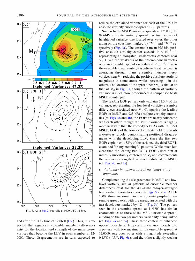
Figures 2 and 3 show the ensemble spread, ensemble
mean, and the two leading EOFs of MSLP that are
identified as the dominant spatial patterns in the en-
semble spread at 11/1800 and 12/0000, respectively.
We see three regions of heightened spread with re-
spect to the ensemble-mean field at 11/1800. The
spread associated with faster-developing ensemble
members (or fast developers for short) is marked by
‘‘M1’’ and symbolizes the creation of pre-TD MSLP
disturbances in some members as demonstrated by the
cluster of PMIN centers (Fig. 2a). Unlike 11/1800,
a bull’s-eye of enhanced spread exists at 12/0000, with
the sample standard deviation exceeding 1 hPa (‘‘M1’’;
Fig. 3a). The overall structure of the ensemble sample
standard deviation evolves into a monopole pattern by
12/0000, but with enhanced spread extending eastward
back toward the West African coastline (‘‘M2’’) in
close proximity to M2 from 11/1800. This eastward
spread is supported by the ensemble-mean MSLP,
which depicts an elongated closed 1008-hPa isobar
extending from the bull’s-eye center back to the
coastline (Fig. 3a).
The largest mode in the ensemble spread at 11/1800 is
depicted by the leading EOF (EOF 1), which explains
29.4% of the variance with a weak monopole pattern
centered near M1 (Fig. 2b). This monopole pattern is
a characteristic of an intensity disagreement between
the ensemble members as demonstrated in previous
studies (Chang et al. 2013; Zheng et al. 2013). Thus, the
3184 JOURNAL OF THE ATMOSPHER IC SC IENCES VOLUME 71
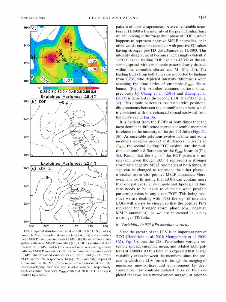
pattern of most disagreement between ensemble mem-
bers at 11/1800 is the intensity of the pre-TD Julia. Since
we are looking at the ‘‘negative’’ phase of EOF 1, which
happens to represent negative MSLP anomalies, or in
other words, ensemble members with positive PC values
having stronger pre-TD disturbances at 11/1800. This
intensity disagreement becomes increasingly evident at
12/0000 as the leading EOF explains 47.3% of the en-
semble spread with a monopole pattern clearly situated
within the ensemble cluster and M1 (Fig. 3b). The
leading EOFs from both times are supported by findings
from CZM, who depicted intensity differences when
assessing the time series of ensemble PMIN distur-
bances (Fig. 1b). Another common pattern shown
previously by Chang et al. (2013) and Zheng et al.
(2013) is depicted in the second EOF at 12/0000 (Fig.
3c). This dipole pattern is associated with positional
disagreements between the ensemble members, which
is consistent with the enhanced spread eastward from
the bull’s-eye in Fig. 3a.
It is evident from the EOFs at both times that the
most dominant difference between ensemble members
is related to the intensity of the pre-TD Julia (Figs. 2b,
3b). As ensemble solutions evolve in time and some
members develop pre-TD disturbances in terms of
PMIN, the second leading EOF evolves into the posi-
tional ensemble differences for the PMIN location (Fig.
3c). Recall that the sign of the EOF pattern is not
relevant. Even though EOF 1 represents a stronger
storm with negative MSLP anomalies at both times, its
sign can be changed to represent the other phase—
a weaker storm with positive MSLP anomalies. More-
over, it is worth noting that EOFs can contain more
than one pattern (e.g., monopole and dipole), and thus,
care needs to be taken to elucidate what possible
pattern(s) exists in any given EOF. This being said,
since we are dealing with TCG the sign of intensity
EOFs will always be chosen so that the positive PC’s
represent the stronger storm phase (e.g., negative
MSLP anomalies), as we are interested in seeing
a stronger TD Julia.
b. Variability in 925-hPa absolute vorticity
Since the growth of the LLV is an important part of
TCG (Hendricks et al. 2004; Montgomery et al. 2006;
CZ), Fig. 4 shows the 925-hPa absolute vorticity en-
semble spread, ensemble mean, and related EOF pat-
terns at 12/0000. At this time, it is expected that a large
variability exists between the members, since the pro-
cess by which the LLV forms is through the merging of
numerous mesovortices and enhancement by deep
convection. The control-simulated TCG of Julia de-
picted that two main mesovortices merge just prior to
FIG. 2. Spatial distributions, valid at 1800 UTC 11 Sep, of (a)
ensemble MSLP standard deviation (shaded, hPa) and ensemble-
meanMSLP (contours, interval of 1 hPa), (b) the most reoccurring
spatial pattern of MSLP anomalies (i.e., EOF 1) contoured with
interval of 0.1 hPa, and (c) the second most reoccurring spatial
pattern of MSLP anomalies (EOF 2) contoured with an interval of
0.1 hPa. The explained variance for (b) EOF 1 and (c) EOF 2 are
29.4% and 22.1%, respectively. In (a), ‘‘M1’’ and ‘‘M2’’ represent
a maximum in the MSLP ensemble spread associated with the
faster-developing members and coastal variance, respectively.
Each ensemble member’s PMIN center at 1800 UTC 11 Sep is
marked by a cross.
SEPTEMBER 2014 CECEL SK I AND ZHANG 3185
and after the TCG time of 12/0600 (CZ). Thus, it is ex-
pected that significant ensemble member differences
exist for the location and strength of the main meso-
vortices that become the LLV in each member at 12/
0000. These disagreements are in turn expected to
reduce the explained variance for each of the 925-hPa
absolute vorticity ensemble-spread EOF patterns.
Similar to the MSLP ensemble spreads at 12/0000, the
925-hPa absolute vorticity spread has two centers of
heightened variance: one located over water, the other
along on the coastline, marked by ‘‘V1’’ and ‘‘V2,’’ re-
spectively (Fig. 4a). The ensemble-mean 925-hPa posi-
tive absolute vorticity center exceeds 9 3 1025 s21,
representing an elongated, weak vortex centered near
V1. Given the weakness of the ensemble-mean vortex
with an ensemble spread exceeding 6 3 1025 s21 near
the ensemble-mean center, it is believed that themean is
averaging through many ensemble member meso-
vortices near V1, reducing the positive absolute vorticity
magnitude in some areas, while increasing it in the
others. The location of the spread near V2 is similar to
that of M2 in Fig. 3a, though the pattern of vorticity
variance is much more pronounced in comparison to its
MSLP counterpart.
The leading EOF pattern only explains 22.3% of the
variance, representing the low-level vorticity ensemble
differences associated near V1. Comparing the leading
EOFs of MSLP and 925-hPa absolute vorticity anoma-
lies (cf. Figs. 3b and 4b), the EOFs are nearly collocated
with each other, though the MSLP variance is slightly
more westward than the vorticity field. As with EOF 2 of
MSLP, EOF 2 of the low-level vorticity field represents
a west–east dipole, demonstrating positional disagree-
ments with the developing LLV. Since the first two
EOFs explain only 38%of the variance, the third EOF is
examined for any meaningful patterns. While much less
clear than the leading two EOFs, EOF 3 does hint at
intensity uncertainty centered on V2 and complements
the west–east-elongated variance exhibited of MSLP
(cf. Figs. 4d and 3a).
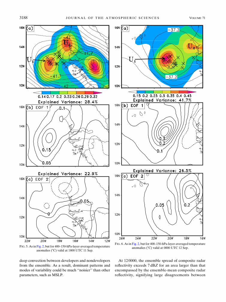
c. Variability in upper-tropospheric temperatureanomalies
Complementing the disagreements in MSLP and low-
level vorticity, similar patterns of ensemble member
differences exist for the 400–150-hPa-layer-averaged
temperature anomalies shown in Figs. 5 and 6. At 11/
1800, three maximum in the upper-tropospheric en-
semble spread exist with the spread associated with the
fast developers marked by ‘‘U1’’ (Fig. 5a). The pattern
seen in the ensemble spread at 11/1800 has similar
characteristics to those of the MSLP ensemble spread,
alluding to the two parameters’ variability being linked
(cf. Figs. 2a and 5a). These three centers of enhanced
upper-tropospheric temperature variance morph into
a pattern with two maxima in the ensemble spread at
12/0000: one over water with a magnitude exceeding
0.458C (‘‘U1’’, Fig. 6a), and the other a slightly weaker
FIG. 3. As in Fig. 2, but valid at 0000 UTC 12 Sep.
3186 JOURNAL OF THE ATMOSPHER IC SC IENCES VOLUME 71
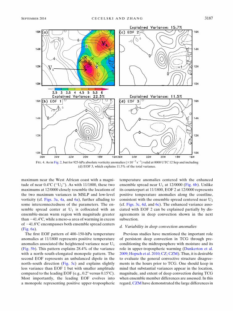
maximum near the West African coast with a magni-
tude of near 0.48C (‘‘U2’’). As with 11/1800, these two
maximums at 12/0000 closely resemble the locations of
the two maximum variances in MSLP and low-level
vorticity (cf. Figs. 3a, 4a, and 6a), further alluding to
some interconnectedness of the parameters. The en-
semble spread center at U1 is collocated with an
ensemble-mean warm region with magnitude greater
than241.48C, while ameso-a area of warming in excess
of241.88C encompasses both ensemble spread centers
(Fig. 6a).
The first EOF pattern of 400–150-hPa temperature
anomalies at 11/1800 represents positive temperature
anomalies associated the heightened variance near U1
(Fig. 5b). This pattern explains 28.4% of the variance
with a north–south-elongated monopole pattern. The
second EOF represents an unbalanced dipole in the
north–south direction (Fig. 5c) and explains slightly
less variance than EOF 1 but with smaller amplitude
compared to the leading EOF (e.g., 0.28 versus 0.158C).Most importantly, the leading EOF evolves into
a monopole representing positive upper-tropospheric
temperature anomalies centered with the enhanced
ensemble spread near U1 at 12/0000 (Fig. 6b). Unlike
its counterpart at 11/1800, EOF 2 at 12/0000 represents
positive temperature anomalies along the coastline,
consistent with the ensemble spread centered near U2
(cf. Figs. 3c, 4d, and 6c). The enhanced variance asso-
ciated with EOF 2 can be explained partially by dis-
agreements in deep convection shown in the next
subsection.
d. Variability in deep convection anomalies
Previous studies have mentioned the important role
of persistent deep convection in TCG through pre-
conditioning the midtroposphere with moisture and its
role in upper-tropospheric warming (Dunkerton et al.
2009; Hopsch et al. 2010; CZ; CZM). Thus, it is desirable
to evaluate the general convective structure disagree-
ments in the hours prior to TCG. One should keep in
mind that substantial variances appear in the location,
magnitude, and extent of deep convection during TCG
when ensemble member differences are assessed. In this
regard, CZMhave demonstrated the large differences in
FIG. 4. As in Fig. 2, but for 925-hPa absolute vorticity anomalies (31025 s21) valid at 0000 UTC 12 Sep and including
(d) EOF 3, which explains 11.5% of the total variance.
SEPTEMBER 2014 CECEL SK I AND ZHANG 3187
deep convection between developers and nondevelopers
from the ensemble. As a result, dominant patterns and
modes of variability could be much ‘‘noisier’’ than other
parameters, such as MSLP.
At 12/0000, the ensemble spread of composite radar
reflectivity exceeds 7 dBZ for an area larger than that
encompassed by the ensemble-mean composite radar
reflectivity, signifying large disagreements between
FIG. 5. As in Fig. 2, but for 400–150-hPa-layer-averaged temperature
anomalies (8C) valid at 1800 UTC 11 Sep.
FIG. 6. As in Fig. 2, but for 400–150-hPa-layer-averaged temperature
anomalies (8C) valid at 0000 UTC 12 Sep.
3188 JOURNAL OF THE ATMOSPHER IC SC IENCES VOLUME 71
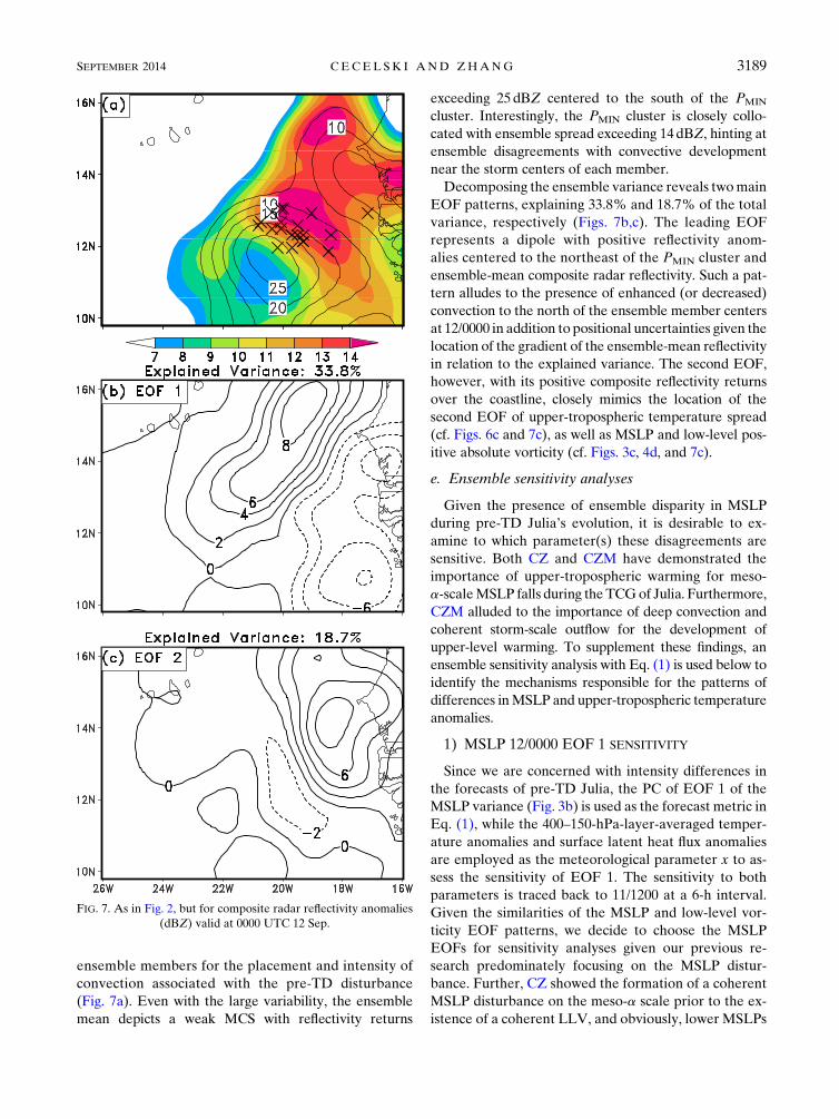
ensemble members for the placement and intensity of
convection associated with the pre-TD disturbance
(Fig. 7a). Even with the large variability, the ensemble
mean depicts a weak MCS with reflectivity returns
exceeding 25dBZ centered to the south of the PMIN
cluster. Interestingly, the PMIN cluster is closely collo-
cated with ensemble spread exceeding 14dBZ, hinting at
ensemble disagreements with convective development
near the storm centers of each member.
Decomposing the ensemble variance reveals twomain
EOF patterns, explaining 33.8% and 18.7% of the total
variance, respectively (Figs. 7b,c). The leading EOF
represents a dipole with positive reflectivity anom-
alies centered to the northeast of the PMIN cluster and
ensemble-mean composite radar reflectivity. Such a pat-
tern alludes to the presence of enhanced (or decreased)
convection to the north of the ensemble member centers
at 12/0000 in addition to positional uncertainties given the
location of the gradient of the ensemble-mean reflectivity
in relation to the explained variance. The second EOF,
however, with its positive composite reflectivity returns
over the coastline, closely mimics the location of the
second EOF of upper-tropospheric temperature spread
(cf. Figs. 6c and 7c), as well as MSLP and low-level pos-
itive absolute vorticity (cf. Figs. 3c, 4d, and 7c).
e. Ensemble sensitivity analyses
Given the presence of ensemble disparity in MSLP
during pre-TD Julia’s evolution, it is desirable to ex-
amine to which parameter(s) these disagreements are
sensitive. Both CZ and CZM have demonstrated the
importance of upper-tropospheric warming for meso-
a-scaleMSLP falls during theTCGof Julia. Furthermore,
CZM alluded to the importance of deep convection and
coherent storm-scale outflow for the development of
upper-level warming. To supplement these findings, an
ensemble sensitivity analysis with Eq. (1) is used below to
identify the mechanisms responsible for the patterns of
differences inMSLP and upper-tropospheric temperature
anomalies.
1) MSLP 12/0000 EOF 1 SENSITIVITY
Since we are concerned with intensity differences in
the forecasts of pre-TD Julia, the PC of EOF 1 of the
MSLP variance (Fig. 3b) is used as the forecast metric in
Eq. (1), while the 400–150-hPa-layer-averaged temper-
ature anomalies and surface latent heat flux anomalies
are employed as the meteorological parameter x to as-
sess the sensitivity of EOF 1. The sensitivity to both
parameters is traced back to 11/1200 at a 6-h interval.
Given the similarities of the MSLP and low-level vor-
ticity EOF patterns, we decide to choose the MSLP
EOFs for sensitivity analyses given our previous re-
search predominately focusing on the MSLP distur-
bance. Further, CZ showed the formation of a coherent
MSLP disturbance on the meso-a scale prior to the ex-
istence of a coherent LLV, and obviously, lower MSLPs
FIG. 7. As in Fig. 2, but for composite radar reflectivity anomalies
(dBZ) valid at 0000 UTC 12 Sep.
SEPTEMBER 2014 CECEL SK I AND ZHANG 3189

enhance PBL convergence, which can enable sub-
sequent growth of the LLV.
As expected, a large positive sensitivity exists between
the PC and upper-tropospheric temperature anomalies
(Fig. 8a), exceeding 0.6 for the Pearson’s correlation.
That is, to reproduce the negative MSLP anomalies
shown in EOF 1 (Fig. 3b), the upper-tropospheric tem-
peratures must increase accordingly. The cluster of en-
semble members whose MSLP minimum are directly
collocated with the statistically significant correlations
supports the importance of upper-tropospheric temper-
ature anomalies forMSLP falls during TCGaswell as the
faster developers at 12/0000 (cf. Figs. 3a, 3b, and 8a).
In contrast, the correlation between the PC and sur-
face latent heat flux anomalies is weaker near the peak
amplitude of EOF 1, though still reaching statistically
significant correlations in collocation with the cluster of
ensemble members (Fig. 8d). Much larger correlations
with the surface heat flux exist well away from the de-
veloping MSLP centers, suggesting stronger winds on
the fringes of the developing low-level circulation
(Fig. 8d). Given the weakness of the wind speeds of the
ensemble at 12/0000, the use of energy from the ocean
surface for intensification of the MSLP disturbance is
unlikely and, thus, the association can be thought of as
substantial variance in the low-level wind speed within
the ensemble.
Tracing the sensitivities back in time, it is evident that
the upper-tropospheric temperature anomalies at 11/
1800 correlate well with the MSLP EOF 1 explained
variance at 12/0000 (Fig. 8b). This is contrasted by the
surface latent heat flux anomalies whose correlation with
the PC quickly diminishes prior to 12/0000 near the en-
semble cluster (Figs. 8e,f). This reduction is as expected,
however, as prior to 12/0000, the sustained surface winds
associated with the pre-TD Julia are mostly below
10m s21 in all ensemble members and they occur mainly
over land (CZM).A stronger correlation to surface latent
heat flux anomalies still exists well west from the storm
centers, again implying increased winds on the fringes of
the developing circulation (Figs. 8e,f). The positive cor-
relation between the upper-tropospheric temperature
anomalies and the PC continues at 11/1200 with a slight
eastward shift toward the coastline (Fig. 8c).
2) UPPER-TROPOSPHERIC TEMPERATURE
12/0000 EOF 1 SENSITIVITY
Figure 9 shows the sensitivity of the leading EOF of
upper-level temperature anomalies to the 400–150-hPa-
layer-averaged relative divergence and composite radar
reflectivity anomalies. We see that near and to the north
of the ensemble cluster center of 236.98C isotherms
strong positive sensitivities occur between the PC of
the leading EOF and 400–150-hPa relative divergence
(Fig. 9a). This result indicates that to reproduce EOF 1
and its positive 400–150-hPa-layer-averaged positive
temperature anomalies, enhanced divergence in the
same layer must occur (e.g., an enhanced storm-scale
outflow). This sensitivity near the storm cluster is the
largest-magnitude correlation within the domain that
the sensitivities are calculated within, suggesting that
there is a physical mechanism behind the correlation
and, thus, do not represent a ‘‘false’’ sensitivity. In
a similar fashion to the relative divergence, strong pos-
itive correlations exist between the PC and composite
radar reflectivity (Fig. 9d). Such a positive correlation
alludes to the need for enhanced convection (positive
composite reflectivity anomalies) to reproduce the
positive temperature anomalies of EOF 1 (cf. Figs. 6b
and 9d). These connections are consistent with CZM,
who noted that enhanced deep convection enabled
a more coherent storm-scale outflow and, thus, an ac-
cumulation of warmth in the upper troposphere as the
Rossby radius of deformation shrinks.
At 11/1800, the sensitivity of the upper-tropospheric
temperature variance to upper-level divergence and
deep convection becomes much less clear. While strong
positive correlations between the leading EOF and di-
vergence appear just off the coastline (Fig. 9b), weak
correlations, if any, exist farther east near the ensemble
cluster. Given that the maximum amplitude of the EOF
is purely situated over water, it is believed that the
positive correlations seen off the coastline in Fig. 9b do
represent the propagation of statistically significant
correlations eastward back in time, for example, with
the propagation of the convective activity. This is further
supported by the physically significant correlations just
off the coastline at 11/1200 (Figs. 9c,f), consistent with
progression of the AEW and embedded convection off
the West African coast.
5. Dominant ensemble differences during theTD stage
As the ensemble solutions evolve, differences between
the ensemble members become increasingly evident. A
schism between developers and nondevelopers was al-
luded to in CZM, who demonstrated distinct differences
in the ensemble when comparing the MSLP disturbances
with upper-tropospheric warming. Even with such a di-
chotomy, 18 of the 20 ensemble members generate a
storm with a PMIN greater than the NHC estimate of
1007hPa (CZM). Furthermore, the ensemble-mean PMIN
of 1004hPa is 1hPa stronger than the control simulation.
This increase in storm intensity spread coexists with fun-
damental changes in the spread of upper-tropospheric
3190 JOURNAL OF THE ATMOSPHER IC SC IENCES VOLUME 71

FIG. 8. Ensemble sensitivity [Eq. (1), shaded] of the 0000 UTC 12 Sep MSLP EOF 1 (Fig. 3b) PC values to
(a)–(c) the 400–150hPa-layer-averaged temperature anomalies; and (d)–(f) surface latent heat flux anomalies (60.42 is
statistically significant at the 95% confidence level). Spaghetti plots for eachmember’sMSLP (black contours, hPa) and
ensemblemean (thick white contour) are overlaid for various isobars. The sensitivities are given at (a),(d) 0000UTC 12
Sep (i.e., the time at which the EOF pattern is valid), (b),(e) 1800 UTC 11 Sep, and (c),(f) 1200 UTC 11 Sep. The
maximum amplitude location of the respective EOF pattern is marked in (a),(d) by a cross.
SEPTEMBER 2014 CECEL SK I AND ZHANG 3191

FIG. 9. As in Fig. 8, but for the leading EOF of the 0000 UTC 12 Sep upper-tropospheric temperature anomalies
(Fig. 6b) and its sensitivity to (a)–(c) 400–150-hPa-layer-averaged relative divergence anomalies and (d)–(f) the
composite radar reflectivity anomalies. The sensitivities depicted in (d)–(f) are only plotted for radar reflectivities
greater than 0 dBZ for all ensemble members and the ensemble mean. Otherwise, the sensitivities are masked out
since convection does not exist (i.e., composite radar reflectivities at or below 0 dBZ). Spaghetti plots for each
member’s 400–150-hPa-layer-averaged temperature (black contours, 8C) and ensemble mean (thick white contour)
are overlaid for various isotherms.
3192 JOURNAL OF THE ATMOSPHER IC SC IENCES VOLUME 71
temperatures and meso-a-scale variability in deep
convection.
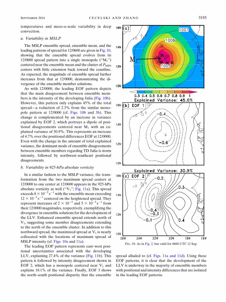
a. Variability in MSLP
The MSLP ensemble spread, ensemble mean, and the
leading patterns of spread for 12/0600 are given in Fig. 10,
showing that the ensemble spread evolves from its
12/0000 spread pattern into a single monopole (‘‘M1’’)
centered near the ensemblemean and the cluster of PMIN
centers with little extension back toward the coastline.
As expected, the magnitude of ensemble spread further
increases from that at 12/0000, demonstrating the di-
vergence of the ensemble member solutions.
As with 12/0000, the leading EOF pattern depicts
that the main disagreement between ensemble mem-
bers is the intensity of the developing Julia (Fig. 10b).
However, this pattern only explains 45% of the total
spread—a reduction of 2.3% from the similar mono-
pole pattern at 12/0000 (cf. Figs. 10b and 3b). This
change is complemented by an increase in variance
explained by EOF 2, which portrays a dipole of posi-
tional disagreements centered near M1 with an ex-
plained variance of 30.9%. This represents an increase
of 4.7% over the positional differences EOF at 12/0000.
Even with the change in the amount of total explained
variance, the dominant mode of ensemble disagreements
between ensemble members regarding TD Julia is storm
intensity, followed by northwest–southeast positional
disagreements.
b. Variability in 925-hPa absolute vorticity
In a similar fashion to the MSLP variance, the trans-
formation from the two maximum spread centers at
12/0000 to one center at 12/0600 appears in the 925-hPa
absolute vorticity as well (‘‘V1’’; Fig. 11a). This spread
exceeds 83 1025 s21 with the ensemble mean exceeding
12 3 1025 s21 centered on the heightened spread. They
represent increases of 2 3 1025 and 5 3 1025 s21 from
their 12/0000 magnitudes, respectively, exemplifying the
divergence in ensemble solutions for the development of
the LLV. Enhanced ensemble spread extends north of
V1, suggesting some member disagreements extending
to the north of the ensemble cluster. In addition to this
northward spread, the maximized spread at V1 is nearly
collocated with the locations of maximum spread of
MSLP intensity (cf. Figs. 10a and 11a).
The leading EOF pattern represents east–west posi-
tional uncertainties associated with the developing
LLV, explaining 27.4% of the variance (Fig. 11b). This
pattern is followed by intensity disagreement shown in
EOF 2, which has a monopole centered near V1 and
explains 18.1% of the variance. Finally, EOF 3 shows
the north–south positional disparity that the ensemble
spread alluded to (cf. Figs. 11a and 11d). Using these
EOF patterns, it is clear that the development of the
LLV is underway in the majority of ensemble members
with positional and intensity differences that are isolated
in the leading EOF patterns.
FIG. 10. As in Fig. 2, but valid for 0600 UTC 12 Sep.
SEPTEMBER 2014 CECEL SK I AND ZHANG 3193

c. Variability in upper-tropospheric temperatureanomalies
An increase in the upper-tropospheric temperature
variability complements the storm intensity disagree-
ments at 12/0600, as shown in Fig. 12a. The ensemble
spread of upper-tropospheric temperature exceeds 0.58C—an increase of 0.058C from the pre-TD stage (cf. Figs. 6a
and 12a). While this increase in spread is notable, the
changes to the spatial characteristics of the spread allude
tomore significant disagreements in the 400–150-hPa-layer-
averaged temperature field between ensemble members.
Instead of the two maxima seen at 12/0000 (Fig. 6a),
a single maximum appears at 12/0600 (see ‘‘U1’’ in Fig.
12a), suggesting that the main disagreement between
the ensemble members is related to the magnitude of
the upper-tropospheric temperature anomalies. Addi-
tionally, the maximum at U1 is directly collocated with
the maximum ensemble spread of MSLP anomalies
(cf. Figs. 10a and 12a) and PMIN cluster, which is con-
sistent with the interconnectedness seen at 12/0000. The
ensemble-mean 400–150-hPa-layer-averaged temperatures
show awarming of approximately 0.58C from 12/0000, with
ameso-a-scale region of warmth centered on the ensemble
spread (Fig. 12a).
The leading EOF pattern of upper-tropospheric tem-
perature anomalies at 12/0600 describes ensemble dif-
ferences on the eastern portion of the ensemble cluster,
with a monopole pattern displaced just east of the max-
imum of ensemble spread (Fig. 12b). This pattern ex-
plains 42.5% of the total variance, an increase over the
41.7% explained by the leading EOF at 12/0000. EOF 2,
explaining 29.2% of the total variance, resembles an
uneven dipole with a positive magnitude pole displaced
westward ofU1 (Fig. 12c).While technically a dipole, it is
clear that EOF 2 resembles more a monopole feature
just west of the center of the largest total variance. The
superposition of these twoEOF patterns represents both
the intensity and positional differences associated with
the 400–150-hPa-layer-averaged temperature anomalies,
with some members displaying an eastward shift in the
positive upper-tropospheric temperature anomalies,
while others depict a westward shift from the center of
maximum total variance. Without the decomposition of
FIG. 11. As in Fig. 2, but for the 925-hPa absolute vorticity (31025 s21) valid for 0600 UTC 12 Sep and including
(d) EOF 3, which explains 14.7% of the total variance.
3194 JOURNAL OF THE ATMOSPHER IC SC IENCES VOLUME 71

the total variance field using EOFs, these characteristics
of the ensemble spread would remain unknown, and
important features of the ensemble differences would
remain overlooked.
d. Variability in deep convection anomalies
As compared to the pre-TD stage, it is evident that the
ensemble-mean composite radar reflectivity exhibits
a weak MCS with maximum radar reflectivity returns
exceeding 30 dBZ, increasing the peak reflectivity by
roughly 5 dBZ from 12/0000 (cf. Figs. 7a and 13a). A
major difference from 12/0000 is that the ensemble clus-
ter of PMIN is collocated at the center of the ensemble-
mean MCS, demonstrating the possibility of substantial
convective development near the storm centers of some
ensemble members (Fig. 13a). However, in a fashion
similar to that at 12/0000, the ensemble spread is maxi-
mized to the north of the ensemble-mean center and
exceeds 14dBZ, signifying substantial disagreement be-
tween the ensemble members on the northern extent of
convective development.
Pulling out the leading EOF yields that the greatest
mode of variability between ensemble members for
composite radar reflectivity anomalies represents pre-
dominately positional disagreements (Fig. 13b). Even
though weak, the uneven magnitude of the dipole de-
picts that the EOF pattern is not purely positional and
includes some intensity differences between ensemble
members. EOF 2 depicts intensity disagreement cen-
tered on the maximum of ensemble spread with a mag-
nitude exceeding 8 dBZ (Fig. 13c). These two patterns
demonstrate that the main ensemble spreads of deep
convection are related to the west–east position, as well
as the strength of deep convection to the north of the
ensemble mean.
e. Ensemble sensitivity analyses
1) MSLP 12/0600 EOF 1 SENSITIVITY
Figure 14 presents the ensemble sensitivity analysis
for PC 1 of MSLP anomalies (Fig. 10b). The instan-
taneous sensitivity (Figs. 14a,d) is strongly positive near
the 1006-hPa ensemble cluster with correlations ex-
ceeding 0.8 for both parameters. A notable increase
from 12/0000 in the instantaneous sensitivity between
the PC and surface latent heat flux anomalies occurs
with correlations exceeding 0.6 for the majority of the
ensemble cluster. This is further evidenced by the sub-
stantially larger region of statistically significant corre-
lations, alluding to the increase in intensity and spatial
extent of the low-level circulation field as exemplified
1009-hPa ensemble cluster (Fig. 14d). The strongest cor-
relations between the PC and upper-tropospheric tem-
perature exist to the southwest of the ensemble cluster,
suggesting enhanced MSLP variance resulting from
the upper-tropospheric temperatures downstream of the
greatest MSLP variance (Fig. 14a). The ensemble-mean
FIG. 12. As in Fig. 2, but for the 400–150-hPa-layer-averaged
temperature anomalies (8C) valid at 0600 UTC 12 Sep.
SEPTEMBER 2014 CECEL SK I AND ZHANG 3195

surfacemaximumwind exceeds 12m s21 and, thus, wind-
induced surface heat exchange (WISHE; Emanuel et al.
1994) can be utilized for generating MSLP falls in the
stronger ensemble members. Since PC 1 is strongly
correlated with both parameters within the ensemble
cluster at 12/0600, we may state that both hydrostatically
induced and WISHE-induced MSLP falls are occurring
and are dependent on the strength of the ensemble
member disturbance.
Tracing the sensitivities back in time, statistically
significant positive correlations between PC 1 and
upper-tropospheric temperature anomalies exist back
until 11/1800 near the ensemble cluster and within
the general larger-scale disturbance encompassed by
the 1010-hPa isobar cluster at 12/0000 (Figs. 14b,c).
On the other hand, the positive correlations between
PC 1 and surface latent heat flux anomalies diminish
quickly, with an indiscernible correlation at 11/1800
(Figs. 14e,f). The most notable reduction of statistically
significant positive correlation exists between 12/0600
and 12/0000 as the most robust correlations are con-
fined to the edges of the developing low-level circula-
tion (Fig. 14e). Some statistically significant correlations
exist with the latent heat flux anomalies near the
ensemble cluster but are much less meaningful when
compared to the upper-tropospheric temperatures (cf.
Figs. 14b and 14e). The reduction in correlations with
surface latent heat flux anomalies makes physical
sense, however, as the ensemble-mean surface maxi-
mum sustained wind speed is below 10m s21 at 11/1800
(CZM) and, thus, the MSLP variance at 12/0600 is
unlikely to be caused by positive surface latent heat flux
anomalies at 11/1800.
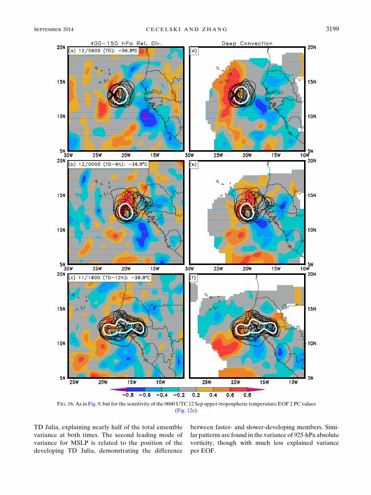
2) UPPER-TROPOSPHERIC TEMPERATURE 12/0600EOF 1 AND 2 SENSITIVITIES
Since both EOFs patterns depicted in Figs. 12b and 12c
represent important features of the upper-temperature
ensemble spread, it is of interest to examine the sensi-
tivity of both EOFs to the 400–150-hPa-layer-averaged
relative divergence and composite radar reflectivity
anomalies.
Figure 15 shows the sensitivity of EOF 1 to upper-
level divergence and deep convection. As at 12/0000,
a strong positive instantaneous sensitivity exists be-
tween the PC of the EOF and both meteorological pa-
rameters near the ensemble cluster and maximum
amplitude of the EOF pattern (see the crosses in Figs.
15a and 15d). These positive sensitivities shift eastward
back in time as the upper-tropospheric temperatures
at 12/0600 are well correlated with enhanced deep
convection and divergence propagating off the West
African coastline. Similar patterns and correlations are
seen for the second EOF (Fig. 12c) with relevant posi-
tive correlations with divergence and composite radar
reflectivity anomalies near the ensemble cluster and
maximum-amplitude location of the EOF (Fig. 16).
FIG. 13. As in Fig. 2, but for the composite radar reflectivity
anomalies (dBZ) valid at 0600 UTC 12 Sep.
3196 JOURNAL OF THE ATMOSPHER IC SC IENCES VOLUME 71

While other sensitivities exist for both EOFs away from
the ensemble clusters, they are generally of less magni-
tude than those of the sensitivities near the cluster and,
thus, yield little, if any, meaningful information on the
implications for the EOF patterns examined.
6. Summary and final thoughts
In this study, we constructed EOFs for multiple pa-
rameters to identify the dominant patterns of ensemble
spreads for the TCG of Hurricane Julia (2010). Using
FIG. 14. As in Fig. 8, but for the sensitivity of the 0600 UTC 12 Sep MSLP EOF 1 (Fig. 10b) PC values.
SEPTEMBER 2014 CECEL SK I AND ZHANG 3197

these parametric patterns of differences, we are able to
make inferences for the dominant mechanisms re-
sponsible for the ensemble spreads and for how each of
the spread of the multiple parameters is connected. Two
main stages were investigated for parametric ensemble
differences: (i) pre-TD stage and (ii) TD stage.
It is found that the dominant pattern of MSLP dis-
agreements is related to the intensity of the pre-TD and
FIG. 15. As in Fig. 9, but for the sensitivity of the 0600 UTC 12 Sep upper-tropospheric temperature EOF 1 PC
values (Fig. 12b).
3198 JOURNAL OF THE ATMOSPHER IC SC IENCES VOLUME 71
TD Julia, explaining nearly half of the total ensemble
variance at both times. The second leading mode of
variance for MSLP is related to the position of the
developing TD Julia, demonstrating the difference
between faster- and slower-developing members. Simi-
lar patterns are found in the variance of 925-hPa absolute
vorticity, though with much less explained variance
per EOF.
FIG. 16. As in Fig. 9, but for the sensitivity of the 0600UTC 12 Sep upper-tropospheric temperature EOF 2 PC values
(Fig. 12c).
SEPTEMBER 2014 CECEL SK I AND ZHANG 3199

The ensemble spread in MSLP and low-level absolute
vorticity is complemented by similar patterns of vari-
ance in upper-tropospheric temperatures, suggesting
that the variances of the variables are linked. At the pre-
TD stage, the maximum of multiple MSLP variance
centers are collocated with centers of the maximum
upper-tropospheric temperature variance. As theMSLP
variance patternmorphs into amonopole pattern during
the TD stage, so does the upper-level temperature var-
iance, closely located to the cluster of ensemble-member
storm centers. Consistent with the pre-TD stage, the
EOFs at the TD stage depict the same characteristics but
characteristic patterns representing faster- and slower-
developing members, instead of just one group of en-
semble members.
To examine what causes the MSLP changes during
TCG, ensemble sensitivity analyses were performed to
compare if upper-tropospheric temperature anomalies
or surface latent heat flux anomalies (i.e., extracting
energy from the ocean surface) are responsible for the
MSLP changes at both stages. At the pre-TD stage,
strong positive sensitivities exist between the upper-
tropospheric temperature anomalies and the EOF rep-
resenting negative MSLP anomalies (e.g., a stronger
pre-TD Julia). This sensitivity is coherent and traceable
back in time, suggesting that to make the pre-TD Julia
stronger, increases in upper-tropospheric temperatures
must occur in the hours prior and at 12/0000. Contrasting
this result, the sensitivity of the EOF pattern to surface
latent heat flux anomalies at the pre-TD stage is less
robust. While some positive correlation exists instan-
taneously, the sensitivity quickly diminishes back in
time. Links between upper-tropospheric temperature
anomalies and deep convection are illustrated through
further ensemble sensitivity analyses. It is evident that
the strength of the upper-level warming during TCG
is positively correlated to enhanced composite radar
reflectivity anomalies (e.g., enhanced deep convection)
and its divergent outflow.
Overall, the results herein paint a more holistic pic-
ture describing the predictability of TCG of Hurricane
Julia through a variety of statistical inferences of im-
portant meteorological parameters for the occurrence of
TCG. The methods herein would benefit other studies
using ensembles to investigate particular meteorological
phenomena, including TCs. Identifying the dominate
characteristics of the ensemble as a whole can provide
a much more robust analysis than investigating and
comparing individual ensemble members. That being
said, the method does have its deficiencies, mainly that
statistical inferences of dynamical processes can yield
unrealistic conclusions or ones that do not adhere to the
governing equations. Regardless of this shortcoming,
the results presented herein provide insight on the
dominant modes of variability occurring during TCG
and elucidate how the variability of multiple parameters
is woven together.
Acknowledgments. This work was supported by
NASAHeadquarters under the NASAEarth and Space
Science Fellowship Program Grant NNX11AP29H and
NASA’s Grant NNX12AJ78G. Model simulations were
performed at the NASA High-End Computing (HEC)
Program through the NASA Center for Climate Simu-
lation (NCCS) at Goddard Space Flight Center.
REFERENCES
Ancell, B., and G. J. Hakim, 2007: Comparing adjoint- and
ensemble-sensitivity analysis with applications to observation
targeting. Mon. Wea. Rev., 135, 4117–4134, doi:10.1175/
2007MWR1904.1.
Braun, S. A., and Coauthors, 2013: NASA’s Genesis and Rapid
Intensification Processes (GRIP) field experiment. Bull. Amer.
Meteor. Soc., 94, 345–363, doi:10.1175/BAMS-D-11-00232.1.
Cecelski, S. F., and D.-L. Zhang, 2013: Genesis of Hurricane Julia
(2010) within anAfrican easterly wave: Low-level vortices and
upper-level warming. J. Atmos. Sci., 70, 3799–3817, doi:10.1175/JAS-D-13-043.1.
——,——, and T.Miyoshi, 2014: Genesis of Hurricane Julia (2010)
within an African easterly wave: Developing and non-
developing members from WRF-LETKF ensemble forecasts.
J. Atmos. Sci., 71, 2763–2781, doi:10.1175/JAS-D-13-0187.1.
Chang, E. K. M., M. Zheng, and K. Raeder, 2013: Medium-range
ensemble sensitivity analysis of two extreme Pacific extra-
tropical cyclones. Mon. Wea. Rev., 141, 211–231, doi:10.1175/MWR-D-11-00304.1.
Dunkerton, T. J., M. T. Montgomery, and Z. Wang, 2009: Tropical
cyclogenesis in a tropical wave critical layer: Easterly waves.
Atmos. Chem. Phys., 9, 5587–5646, doi:10.5194/acp-9-5587-2009.
Emanuel, K. A., J. D. Neelin, and C. S. Bretherton, 1994: On large-
scale circulations in convecting atmospheres. Quart. J. Roy.
Meteor. Soc., 120, 1111–1144, doi:10.1002/qj.49712051902.Gombos, D., R. N. Hoffman, and J. A. Hansen, 2012: Ensemble
statistics for diagnosing dynamics: Tropical cyclone track
forecast sensitivities revealed by ensemble regression. Mon.
Wea. Rev., 140, 2647–2669, doi:10.1175/MWR-D-11-00002.1.
Hawblitzel, D. P., F. Zhang, Z. Meng, and C. A. Davis, 2007:
Probabilistic evaluation of the dynamics and predictability of
the mesoscale convective vortex of 10–13 June 2003. Mon.
Wea. Rev., 135, 1544–1563, doi:10.1175/MWR3346.1.
Hendricks, E. A., M. T. Montgomery, and C. A. Davis, 2004: The
role of ‘‘vortical’’ hot towers in the formation of Tropical
Cyclone Diana (1984). J. Atmos. Sci., 61, 1209–1232,
doi:10.1175/1520-0469(2004)061,1209:TROVHT.2.0.CO;2.
Hopsch, S. B., C. D. Thorncroft, and K. R. Tyle, 2010: Analysis of
African easterly wave structures and their role in influencing
tropical cyclogenesis. Mon. Wea. Rev., 138, 1399–1419,
doi:10.1175/2009MWR2760.1.
Houze, R. A., W.-C. Lee, and M. M. Bell, 2009: Convective con-
tribution to the genesis of Hurricane Ophelia (2005). Mon.
Wea. Rev., 137, 2778–2800, doi:10.1175/2009MWR2727.1.
Hunt, B. R., E. J. Kostelich, and I. Szunyogh, 2007: Efficient data
assimilation for spatiotemporal chaos: A local ensemble
3200 JOURNAL OF THE ATMOSPHER IC SC IENCES VOLUME 71
transformKalman filter. Physica D, 230, 112–126, doi:10.1016/
j.physd.2006.11.008.
Miyoshi, T., and M. Kunii, 2012: The local ensemble transform
Kalman filter with the weather research and forecasting
model: Experiments with real observations. Pure Appl. Geo-
phys., 169, 321–333, doi:10.1007/s00024-011-0373-4.
Montgomery,M. T.,M. E. Nicholls, T.A. Cram, andA.B. Saunders,
2006: A vortical hot tower route to tropical cyclogenesis.
J. Atmos. Sci., 63, 355–386, doi:10.1175/JAS3604.1.
——, L. L. Lussier III, R. W. Moore, and Z. Wang, 2010: The
genesis of Typhoon Nuri as observed during the Tropical
Cyclone Structure 2008 (TCS-08) field experiment—Part 1:
The role of the easterly wave critical layer. Atmos. Chem.
Phys., 10, 9879–9900, doi:10.5194/acp-10-9879-2010.
——, and Coauthors, 2012: The Pre-Depression Investigation of
Cloud-Systems in the Tropics (PREDICT) experiment: Scien-
tific basis, new analysis tools, and some first results.Bull. Amer.
Meteor. Soc., 93, 153–172, doi:10.1175/BAMS-D-11-00046.1.
Sippel, J. A., and F. Zhang, 2008: A probabilistic analysis of the
dynamics and predictability of tropical cyclogenesis. J. Atmos.
Sci., 65, 3440–3459, doi:10.1175/2008JAS2597.1.
——, J. W. Nielsen-Gammon, and S. E. Allen, 2006: The multiple-
vortex nature of tropical cyclogenesis. Mon. Wea. Rev., 134,
1796–1814, doi:10.1175/MWR3165.1.
Torn, R. D., and G. J. Hakim, 2008: Ensemble-based sensitivity
analysis. Mon. Wea. Rev., 136, 663–677, doi:10.1175/
2007MWR2132.1.
——, and D. Cook, 2013: The role of vortex and environment
errors in genesis forecasts of Hurricanes Danielle and
Karl (2010). Mon. Wea. Rev., 141, 232–251, doi:10.1175/
MWR-D-12-00086.1.
Wang, Z., M. T. Montgomery, and T. J. Dunkerton, 2010: Genesis
of pre–Hurricane Felix (2007). Part I: The role of the easterly
wave critical layer. J. Atmos. Sci., 67, 1711–1729, doi:10.1175/
2009JAS3420.1.
Zhang, D.-L., and L. Zhu, 2012: Roles of upper-level processes in
tropical cyclogenesis. Geophys. Res. Lett., 39, L17804,
doi:10.1029/2012GL053140.
Zheng, M., E. K. M. Chang, and B. A. Colle, 2013: Ensemble
sensitivity tools for assessing extratropical cyclone intensity
and track predictability. Wea. Forecasting, 28, 1133–1156,
doi:10.1175/WAF-D-12-00132.1.
SEPTEMBER 2014 CECEL SK I AND ZHANG 3201
Recommended