9
1.0 INTRODUCTIONThis report presents the findings of a field project undertaken in the west and south
Gippsland region of Victoria between May and December 2002. The work is a
component of the larger Gippsland Dairy Riparian Project funded by the Dairy
Research and Development Corporation and GippsDairy. The aim of the larger
project is to determine, demonstrate and communicate Best Management Practices for
riparian habitats in landscapes dominated by dairy farming.
In this project, we surveyed 107 sites and conducted 28 landholder interviews to gain
information on the variation in the ecological condition of riparian habitats and
management practices among farmers in the west and south Gippsland region. The
specific aims of the project were:
� To determine the current condition of riparian habitats across the west and south
Gippsland dairy region.
� To investigate the relationships between landholder management practices and
riparian condition.
� To make recommendations for management practices that could be investigated at
demonstration sites planned for the region.
2.0 BACKGROUND
2.1 Dairy industry in west and south Gippsland
Australian dairy farmers support an industry with an annual value of $3 billion. As
part of their plan for the future the Australian dairy industry has made the
management and preservation of natural resources one of it’s highest priorities. The
recent review of the industry provided in the report ‘Sustaining Our Natural
Resources – Dairying for Tomorrow’ highlighted the industry’s desire to sustain
natural resources while increasing productivity in the context of a highly competitive
market (Anon. 2001). The Dairying for Tomorrow report contains a national strategy
and eight regional action plans for resource management in Australia’s recognised
dairying areas. The national strategy also provided guidelines for generic best practice
management of major resources and processes under the headings: Water, Land, Soil
Conservation, Nutrient run-off, Effluent and Biodiversity.
10
Victorian dairy farmers account for a major portion of the Australian dairy industry’s
annual milk production and approximately 60% of the industry’s farms are located in
Victoria. Much of the state’s primary dairy production is focused in the Gippsland
region1, east of Melbourne. Approximately $1.2 billion worth of exports come from
this region annually (Anon. 2001).
Total production in the Gippsland region expected to increase by 50% in the next 10
years (Anon. 2001), consequently the implementation of sound management practices
that target both environmental and production issues are vital to the future of the
region’s dairy industry. Historical clearing of steep catchments and the intensive
nature of the production systems (high stocking rates and fertiliser application on
small farms with small economic margins) combined with high rainfalls (1000-2000
mm per year) have combined to produce a region with severely impaired landscape
functions. Land slippage is common on steep slopes. A reduction of biodiversity has
occurred as a consequence of removal, fragmentation and reductions in the quality of
habitats. Subsequently 60% of the waterways in west Gippsland are estimated to be in
poor to very poor condition (Anon. 2001).
The Gippsland Regional Action Plan (GippsDairy 2001) was developed as a joint
venture between the GippsDairy Regional Development Program and the West
Gippsland Catchment Management Authority (WGCMA). The action plan aims to
maintain productivity while promoting an environmentally sustainable industry. The
key resource management issues for the region’s dairy industry were identified as:
� Development of whole farm plans
� Managing land use change and local planning
� Achieving sustainable productivity gains
� Increasing water use efficiency
� Nutrient management
� Effluent management
� Increasing biodiversity
1 Milk production in Gippsland comes from two major regions: west and southGippsland. Farms are located in the Strezlecki Ranges and on the Gippsland Plain,and east Gippsland where production is focused on the Gippsland Plain with a largenumber of farms supported by irrigation (Anon. 2001).
11
� Land protection
Many of these issues are closely related to the appropriate management of the
boundaries between paddocks and waterways on farms, i.e. riparian habitats.
Despite the availability of generic management recommendations for riparian habitats
(e.g. Anon. 2001) and the information that resides with individual farmers, catchment
coordinators and agency staff in the Gippsland region, there is little specific
information available to dairy farmers in Gippsland regarding best management
practices for their riparian areas. This lack of information has been recognised by the
dairy industry as an impediment to successful management:
A more scientifically based appreciation of how such measures (fencing toexclude stock) also contribute to the health of aquatic systems would be ofvalue. There is a need to better appreciate the direct impact of farmmanagement practices on the health of catchments (Anon. 2001, pp40).
For the Gippsland Regional Action Plan (GippsDairy 2001) to be implemented
successfully, scientific information specific to the dairy regions needs to form the
basis for extension programs for the sustainable management of waterways. For this
reason the Dairy Research and Development Corporation and GippsDairy combined
to support the larger Gippsland Dairy Riparian Project, of which this current project is
a part.
2.2 Identifying Best Management Practices for riparian habitats inthe west and south Gippsland dairy region
Recommendations for the appropriate management of livestock in riparian habitats in
dryland regions of Australia typically includes provision of off-river water supplies,
rotational grazing practices where access to riparian areas occurs infrequently for
short periods, strategic fencing of parts of the riparian zone combined with replanting
of native species, and the retention of grass buffer strips to intercept runoff and
minimise inputs to streams (MacLeod 2002). There is now good evidence that the
application of these approaches can result in significant increases in the condition of
riparian habitats without impacting on the economic viability of grazing enterprises
(Jansen & Robertson 2001a, Curtis et al. 2001).

12
However, it is unknown to what degree such management initiatives will be effective
or acceptable to dairy farmers in the very different landscape and economic situations
in Gippsland.
2.3. This studyIn this study we used rapid assessments (e.g. Jansen & Robertson 2001a) at a large
number of sites to provide information on riparian condition and farm management
specific to west and south Gippsland dairy farms. We collected information on the
current status of riparian habitats in the two major bioregions (DPI 2002) of west and
south Gippsland (Strezlecki Ranges and the Gippsland Plain). Riparian habitats in
these bioregions were further divided into those that had received riparian
management initiatives in the form of exclusion of stock, and those that had not. By
linking the information on riparian condition with information on current management
of dairy farms obtained by interviewing landholders we were able to investigate how
different practices influenced the condition of riparian habitats, and therefore identify
possible best practices.
3.0 METHODS
3.1 Study Region
The study area was located within the west and south Gippsland dairy regions of
southeastern Victoria. All sites were within the areas governed by the West Gippsland
Catchment Management Authority (WGCMA). The WGCMA boundaries extend
from the alpine areas below Mansfield in the north to Wilson’s Promontory in the
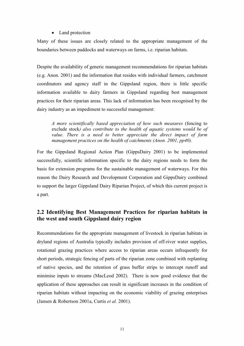
south and from Warragul in the west to Sale in the east (see Figure 1). West
Gippsland is divided into 3 state-recognised river basins; the Latrobe and Thomson
basins, which flow to Lake Wellington in the east, and the South Gippsland basin that
flows to the southern coast and adjacent inlets.
.

13
14
Figure 1. Map of the study area showing the south and west Gippsland dairy regions and thelocation of the survey sites and reference sites. Some dot points are indistinguishable as theyare close together.

15
Industry in the area is dominated by those that draw directly from the region’s natural
resources (e.g. agriculture, electricity and forestry) with the region being the most
densely settled area in the state outside metropolitan Melbourne (Waterwatch 2000).
Agriculture is dominated by dryland pasture farming usually of dairy and beef cows.
Dairy farming in the region began in the mid 1800’s with extensive clearing
throughout the catchment continuing well in to the 1950’s (Anon. n.d.). The average
herd size is 166 milking cows. This number is steadily increasing as smaller farms
succumb to competition from larger farms and the difficulties of farming small
acreage on steep land.
The area experiences warm dry summers (average maximum 24.0 ºC in January) and
cold wet winters (average maximum 12.2 ºC in July). The study area takes in the
designated bioregions of the Gippsland Plain and the Strezlecki Ranges. Mean annual
rainfall ranges from approximately 900mm in the drier Gippsland Plain up to
2000mm in the much wetter Strezlecki Ranges (Bureau of Meteorology 2003).
Topography varies significantly across the two bioregions. The Gippsland Plain
includes lowland coastal and alluvial plains characterised by gently undulating terrain,
while the Strezlecki Ranges consists of moderate to steep slopes with deeply dissected
blocks of sandstone, siltstone and shales (DPI 2002). The rich soils support wet and
damp forests as well as shrubby foothill forest.
Each bioregion has distinctly different vegetation communities and consist of
different Ecological Vegetation Classes (EVC’s). Each EVC represents one or more
floristic communities that occur in similar types of environments and tend to show
similar ecological responses to environmental disturbance (DPI 2002). Each bioregion
has dominant known and expected (pre 1750’s) EVC’s.
The Gippsland Plain is dominated by the Lowland Forest EVC. The floristic
community of this EVC is severely depleted due to intensive clearing for agriculture.
Soils vary from damp sands to sandy topsoils over gravel or clay subsoils. Dominant
overstorey vegetation includes White Stringybark (Eucalyptus globoidea), Narrow-
leaf Peppermint (Eucalyptus radiata), Blackwood (Acacia melanoxylon) and Silver
Wattle (Acacia dealbata). Austral Bracken (Pteridium esculentum), Kangaroo Grass
16
(Themeda triandra) and various Tussock species (Poa spp.) would have dominated
the dense groundcover (RFA 1999). (See Appendix 1a for detailed species list and
EVC description).
The Strezlecki bioregion supports three major EVC’s being Wet Forest, Damp Forest
and Shrubby Foothill Forest. The Wet and Damp Forest EVC’s support similar
floristic communities with Wet Forest more common on topographically protected
high rainfall areas and headwaters of south flowing streams and Damp Forest (see
Appendix 1b) extending to lower elevations and rainfall areas. Dominant eucalypts
include Messmate (Eucalyptus obliqua), Mountain Grey Gum (Eucalyptus
cypellocarpa) and Blackwood (Acacia melanoxylon) with Mountain Ash (Eucalyptus
regnans) more dominant in Wet Forests (see Appendix 1c). Typical understoreys
include a variety of moisture dependent fern species such as Rough Tree fern
(Cyathea australis), Soft Tree fern (Dicksonia antarctica), Common Ground fern
(Calochlaena dubia) and Mother Shield fern (Polystichum proliferum) (RFA 1999).
Shrubby Foothill Forest occurs in habitats at the drier end of Damp Forest on fertile
well-drained soils. This EVC is dominated by overstorey species of Narrow-leaf
Peppermint (Eucalyptus radiata), Messmate (Eucalyptus obliqua) and Mountain Grey
Gum (Eucalyptus cypellocarpa). Ground cover is very species poor and includes
Austral Bracken (Pteridium esculentum) and Tall Sword-sedge (Lepidosperma
elatius) (RFA 1999) (see Appendix 1d).
3.2 Study designAll sites were riparian areas on dairy farms with no major irrigation. Sites were
divided into stream size categories; tributaries and small creeks (1st - 2nd order
streams), and large creek and rivers (≥3rd order streams). In most cases small stream
sizes occurred in the Strezlecki Ranges (hilly) bioregion and larger creeks and rivers
occurred on the Gippsland Plain (flats). These two stream size categories were then
each further spilt into two site categories: a) remnant or planted and b) grazed (see
Figure 2).

17
Although the study involved a balanced design, site selection was random within each
of the four final categories. Size of creeks and their current management were not
known until arrival at the site.
Figure 2. A summary of the study design. Each of the 4 bottom level groupscontained 25-30 individual riparian sites (n=107).
Twenty-eight individual farmers were interviewed in relation to current and past on-
farm management practices. Participants were chosen randomly with all farmers
answering the same questions set prior to the interview being conducted. Although
farmers were chosen randomly some declined to participate in the interview due to
time constraints on the farm (interview time was approximately 1hour).
Surveys of riparian condition were conducted at 107 sites between June and
November. Condition index measurements included measures of habitat, cover,
debris, natives and species (see section 3.4 later). Of the 107 sites for which riparian
condition was measured 38 were linked to farmer interview data as some of the
interviewed farmers had more than one riparian area.
3.3 Landholder interviewsInterviews were conducted with 28 different landholders. Interview questions
pertained to both past and present on-farm management practices and did not include
any questions relating to social aspects of riparian management (e.g. farmer
perceptions of riparian areas, why they are important, why restoration has or hasn’t
been attempted).
remnant orreplanted
grazing
creeks, tributaries(small)
remant orreplanted
grazing
rivers(large)
Riparian zones with no major irrigation
18
Questions were divided into 5 broad categories. 1) General questions that included
questions about farm size, ownership and past land use. 2) Stocking rates and paddock
sizes with questions about the break up of current stocking rates, past stocking rates,
number and size of paddocks and rotational grazing practices employed. 3)
Streambanks and watering points that included questions about flooding, numbers of
riparian paddocks, total length of creek/river frontage, riparian restoration (if any) and
weed management techniques. 4) Effluent, irrigation and stock loss that included
methods and frequency of irrigation, types of effluent systems and management of
effluent and loss of stock in creek/river associated areas. 5) Conservation and new
management regimes, which included questions about any new management that has
resulted in an improved farm environment, whether this new management was cost
positive and if they were members of Landcare (see Appendix 2 for full interview).
3.4 Ecological condition and rapid appraisalOwing to the spatial scales of human impacts on the landscape and the need for
assessment of ecological change, there is an expanding field of research focused on
rapid appraisal techniques to measure ecosystem condition or integrity (Fairweather
1999; Boulton 1999). Condition refers to the degree to which human-altered
ecosystems diverge from local semi-natural ecosystems in their ability to support a
community of organisms and perform ecological functions (Karr 1999).
In order to investigate the condition of riparian areas on private properties, we used
rapid surveys of the ecological condition of riparian habitats (Appendix 3). During the
surveys we obtained measures for a number of indicator variables that are linked to
physical, biotic community and landscape functions of riparian habitats (Table 1).
Recently, Jansen and Robertson (2001a) developed and tested an index for the rapid
appraisal of the ecological condition of riparian and floodplain habitats on the
Murrumbidgee River using a sub-set of the indicators proposed by Ladson et al.
(1999). The index was made up of six sub-indices, each with a number of indicator
variables. In this study, we used an amended version of the Jansen and Robertson
(2001a) index with five sub-indices as shown in Appendix 4. The five sub-indices
19
included in the rapid assessment were: (1) width and longitudinal continuity of
vegetation, (2) vegetation cover and structural complexity, (3) standing and fallen
debris, (4) dominance of natives vs exotics, and (5) a series of special features
including regeneration of canopy species, presence or absence of reeds and tree ferns
and weed species declared noxious for the region.
In order to choose appropriate indicator variables for each of the sub-indices and to
set appropriate scores for indicators we used seven reference sites across the west and
south Gippsland regions (Table 2). The two major criteria used for choosing reference
sites were: (1) that riparian vegetation structure was similar to that expected for the
pre 1750 Ecological Vegetation Classes (see RFA 1999 and Appendix 1a-d) in the
two bioregions of west and south Gippsland (Gippsland Plain, Strezlecki Ranges), and
(2) where domestic livestock had been excluded from the site for more than 15 years.
On the basis of the observed vegetation structure at the reference sites, where there
were four distinct layers (upper canopy, sub-canopy, understorey and ground cover)
we increased the number of variables in the sub-index vegetation cover from three in
the original index (Jansen & Robertson 2001a) to four for the Gippsland surveys. In
addition, owing to the shading provided by the well-developed canopies and sub-
canopies in the riparian habitats in the Strezlecki bioregion, (RFA 1999) we adjusted
the scoring for the groundcover layer for all HILLY sites to 0=absent or 1=present.
Scores for both HILLY and FLAT sites were scaled to scores out of 50 so that
comparisons could be made across the region (see Appendix 4).
Note that choice as a reference site did not mean that the vegetation species
composition was equivalent to the Ecological Vegetation Classes (see RFA 1999; DPI
2002) expected for these sites. This was because most sites had significant numbers of
exotic plant species and some had significant understories of noxious weeds. Thus
while they allowed us to establish indicators and scores for the rapid appraisal index
based on structural attributes of the vegetation they did not score the maximum value
for condition using the rapid appraisal index (see later).
20
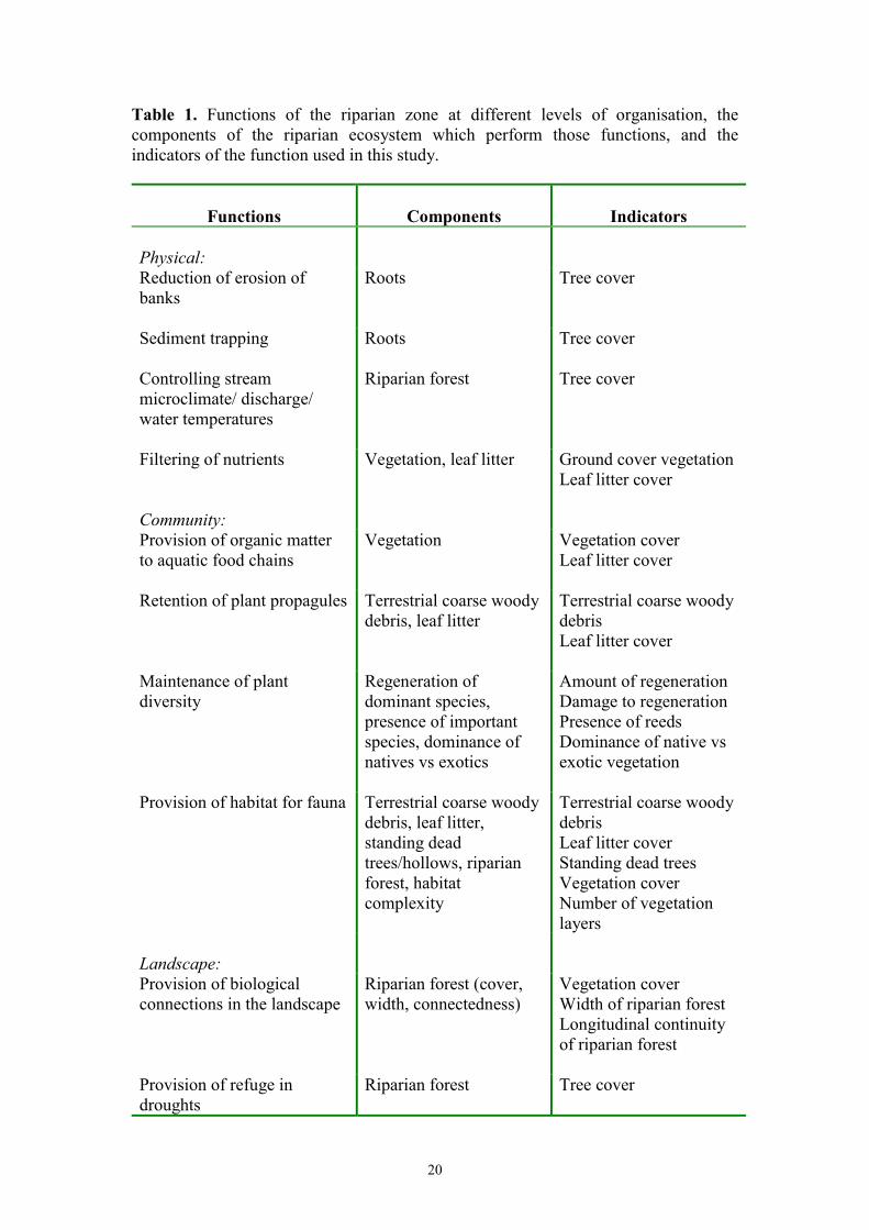
Table 1. Functions of the riparian zone at different levels of organisation, thecomponents of the riparian ecosystem which perform those functions, and theindicators of the function used in this study.
Functions Components Indicators
Physical:Reduction of erosion ofbanks
Roots Tree cover
Sediment trapping Roots Tree cover
Controlling streammicroclimate/ discharge/water temperatures
Riparian forest Tree cover
Filtering of nutrients Vegetation, leaf litter Ground cover vegetationLeaf litter cover
Community:Provision of organic matterto aquatic food chains
Vegetation Vegetation coverLeaf litter cover
Retention of plant propagules Terrestrial coarse woodydebris, leaf litter
Terrestrial coarse woodydebrisLeaf litter cover
Maintenance of plantdiversity
Regeneration ofdominant species,presence of importantspecies, dominance ofnatives vs exotics
Amount of regenerationDamage to regenerationPresence of reedsDominance of native vsexotic vegetation
Provision of habitat for fauna Terrestrial coarse woodydebris, leaf litter,standing deadtrees/hollows, riparianforest, habitatcomplexity
Terrestrial coarse woodydebrisLeaf litter coverStanding dead treesVegetation coverNumber of vegetationlayers
Landscape:Provision of biologicalconnections in the landscape
Riparian forest (cover,width, connectedness)
Vegetation coverWidth of riparian forestLongitudinal continuityof riparian forest
Provision of refuge indroughts
Riparian forest Tree cover
21
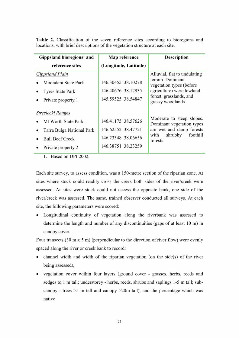
Table 2. Classification of the seven reference sites according to bioregions andlocations, with brief descriptions of the vegetation structure at each site.
Gippsland bioregions1 and
reference sites
Map reference
(Longitude, Latitude)
Description
Gippsland Plain
� Moondara State Park
� Tyres State Park
� Private property 1
146.30455 38.10278
146.40676 38.12935
145.59525 38.54847
Alluvial, flat to undulatingterrain. Dominantvegetation types (beforeagriculture) were lowlandforest, grasslands, andgrassy woodlands.
Strezlecki Ranges
� Mt Worth State Park
� Tarra Bulga National Park
� Bull Beef Creek
� Private property 2
146.41175 38.57626
146.62552 38.47721
146.23348 38.06656
146.38751 38.23259
Moderate to steep slopes.Dominant vegetation typesare wet and damp forestswith shrubby foothillforests
1. Based on DPI 2002.
Each site survey, to assess condition, was a 150-metre section of the riparian zone. At
sites where stock could readily cross the creek both sides of the river/creek were
assessed. At sites were stock could not access the opposite bank, one side of the
river/creek was assessed. The same, trained observer conducted all surveys. At each
site, the following parameters were scored:
� Longitudinal continuity of vegetation along the riverbank was assessed to
determine the length and number of any discontinuities (gaps of at least 10 m) in
canopy cover.
Four transects (30 m x 5 m) (perpendicular to the direction of river flow) were evenly
spaced along the river or creek bank to record:
� channel width and width of the riparian vegetation (on the side(s) of the river
being assessed),
� vegetation cover within four layers (ground cover - grasses, herbs, reeds and
sedges to 1 m tall; understorey - herbs, reeds, shrubs and saplings 1-5 m tall; sub-
canopy - trees >5 m tall and canopy >20m tall), and the percentage which was
native
22
� the number of vegetation layers,
� leaf litter cover on the ground and the percentage which was native species,
� the presence or absence of standing dead trees (snags),
� the abundance of coarse woody debris (>10 cm in diameter) and the percentage
which was native species,
� abundance of canopy species seedlings (<1 m tall),
� grazing damage to canopy species seedlings,
� the presence or absence of reeds and tree ferns, and
� the number of species of declared noxious weeds for the region.
Because livestock concentrate their activities at land-water interfaces, stocking rates
may not be the best estimate of livestock impact on riparian areas (Robertson 1997).
In this study, cowpat counts were used as an index of cattle activity at each site.
Cowpats were counted within the four 30 metre transects and within 1 metre of the
line on each transect.
At each site estimates for each indicator were averaged, scored and weighted, then
summed to give a total score (see Appendix 4). Potential scores for the total condition
index ranged from 0 (worst condition) to 50 (best condition). In order to summarise
some of our results, we grouped total condition scores for surveyed sites into five
categories, as follows: very poor condition <25, poor condition �25<30, average
condition �30<35, good condition �35<40, and excellent condition �40. Correlations
between variables were tested using Pearson’s correlation coefficient (r).
As part of the study we wanted to determine whether a condition index score based on
assessment of riverbank vegetation and litter provided a proxy assessment of in-
stream condition. Measures of in-stream metabolism (daily rates of primary
production (P) and respiration (R) for stream sediments and resultant P:R ratios to
assess net autotrophy or heterotrophy) have been found to provide excellent indicators
of in-stream “health” (Bunn et al. 1999). At a sub-set of 20 riparian sites in Gippsland
where we had information to calculate the index of riparian condition we measured
in-stream metabolism using the methods and equipment described in Bunn et al.
1999. The sites were chosen to represent a range of condition scores, stream sizes and

23
spread evenly over the two bioregions. Regressions of in-stream metabolism on
condition index scores (and sub-index scores) showed many significant relationships
(see Appendix 5).
Another aspect of the study was determining the relationship between the riparian
condition index scores, grazing impacts and riparian bird communities. There were
two reasons for this: (1) A significant impact of grazing on riparian bird communities,
and a significant relationship between riparian condition and bird communities would
suggest that grazing, and associated decline in riparian health, is having far-reaching
impacts on native bird populations in the region; and (2) A relationship between
riparian condition and bird communities suggests the possibility that some bird
species might be used as indicators of the success of altered land management
practices to restore riparian areas. We recorded all birds seen and heard in the riparian
zone during surveys to assess riparian condition scores. Each survey was completed in
approximately thirty minutes, and covered an area of approximately 150x50m. For
this preliminary study, only one survey was conducted at each site.
To examine the effects of grazing and riparian condition on the bird communities
recorded at each site, we used Distance-based Multivariate Analysis for a Linear
Model (Anderson 2001), and to illustrate how bird communities varied according to
riparian condition, we used Non-metric Multi-dimensional Scaling in PRIMER
(Clarke 1993). All analyses were done on presence-absence data, and similarities
between sites were calculated using the Bray-Curtis metric. A Similarity Percentages
Analysis was conducted in PRIMER (Clarke & Warwick 1994) to determine those
bird species characteristic of riparian sites in poor and good condition. The results of
these analyses are presented in Appendix 6.
24
4.0 RESULTS
4.1 Dairy farmer interviews
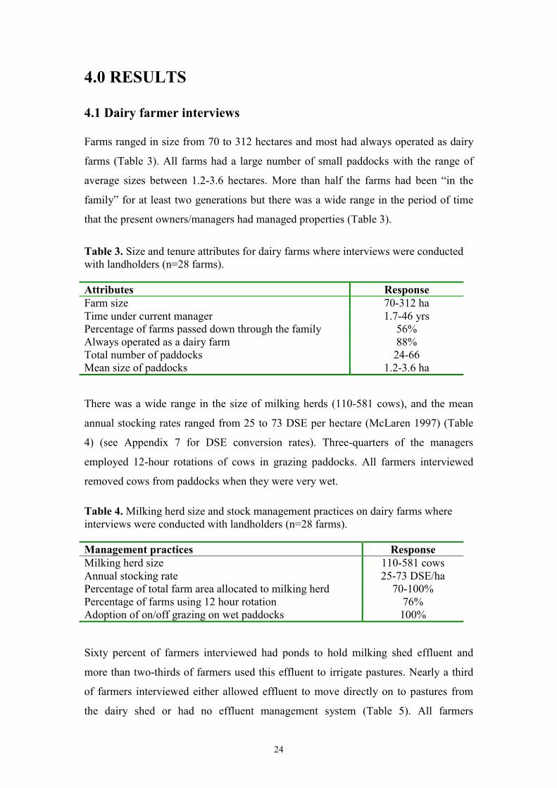
Farms ranged in size from 70 to 312 hectares and most had always operated as dairy
farms (Table 3). All farms had a large number of small paddocks with the range of
average sizes between 1.2-3.6 hectares. More than half the farms had been “in the
family” for at least two generations but there was a wide range in the period of time
that the present owners/managers had managed properties (Table 3).
Table 3. Size and tenure attributes for dairy farms where interviews were conductedwith landholders (n=28 farms).
Attributes ResponseFarm size 70-312 haTime under current manager 1.7-46 yrsPercentage of farms passed down through the family 56%Always operated as a dairy farm 88%Total number of paddocks 24-66Mean size of paddocks 1.2-3.6 ha
There was a wide range in the size of milking herds (110-581 cows), and the mean
annual stocking rates ranged from 25 to 73 DSE per hectare (McLaren 1997) (Table
4) (see Appendix 7 for DSE conversion rates). Three-quarters of the managers
employed 12-hour rotations of cows in grazing paddocks. All farmers interviewed
removed cows from paddocks when they were very wet.
Table 4. Milking herd size and stock management practices on dairy farms whereinterviews were conducted with landholders (n=28 farms).
Management practices ResponseMilking herd size 110-581 cowsAnnual stocking rate 25-73 DSE/haPercentage of total farm area allocated to milking herd 70-100%Percentage of farms using 12 hour rotation 76%Adoption of on/off grazing on wet paddocks 100%
Sixty percent of farmers interviewed had ponds to hold milking shed effluent and
more than two-thirds of farmers used this effluent to irrigate pastures. Nearly a third
of farmers interviewed either allowed effluent to move directly on to pastures from
the dairy shed or had no effluent management system (Table 5). All farmers
25
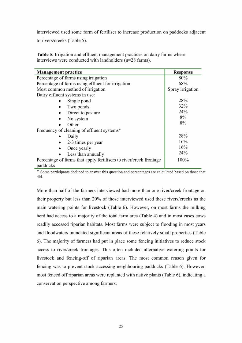
interviewed used some form of fertiliser to increase production on paddocks adjacent
to rivers/creeks (Table 5).
Table 5. Irrigation and effluent management practices on dairy farms whereinterviews were conducted with landholders (n=28 farms).
Management practice ResponsePercentage of farms using irrigation 80%Percentage of farms using effluent for irrigation 68%Most common method of irrigation Spray irrigationDairy effluent systems in use:
� Single pond� Two ponds� Direct to pasture� No system� Other
28%32%24%8%8%
Frequency of cleaning of effluent systems*� Daily� 2-3 times per year� Once yearly� Less than annually
28%16%16%24%
Percentage of farms that apply fertilisers to river/creek frontagepaddocks
100%
* Some participants declined to answer this question and percentages are calculated based on those thatdid.
More than half of the farmers interviewed had more than one river/creek frontage on
their property but less than 20% of those interviewed used these rivers/creeks as the
main watering points for livestock (Table 6). However, on most farms the milking
herd had access to a majority of the total farm area (Table 4) and in most cases cows
readily accessed riparian habitats. Most farms were subject to flooding in most years
and floodwaters inundated significant areas of these relatively small properties (Table
6). The majority of farmers had put in place some fencing initiatives to reduce stock
access to river/creek frontages. This often included alternative watering points for
livestock and fencing-off of riparian areas. The most common reason given for
fencing was to prevent stock accessing neighbouring paddocks (Table 6). However,
most fenced off riparian areas were replanted with native plants (Table 6), indicating a
conservation perspective among farmers.

26
Table 6. Attributes of river/creek frontages and management practices related toriparian areas on dairy farms where interviews were conducted with landholders(n=28 farms).
Management practice ResponsePercentage of farms affected by flooding 60%Distance floodwaters can reach laterally from creek bed 20-500mMean distance from river/creek frontage to other watering points 40-400mPercentage of farms with more than one river/creek frontage 56%Percentage of farms that use river/creek as main watering points 16%Percentage of farms with some fenced river/creek frontage 84%Percentage of fenced areas replanted with trees 76%Most common reason for fencing river/creek frontage Prevent stock
accessingneighbouring
paddocksMost common method of weed management in fenced areas Spot sprayingPercentage of farms where fencing river/creek frontage reducedtime required for stock management
72%
Nearly three-quarters of farmers interviewed indicated that fencing of riparian areas
resulted in a significant time saving in stock management, and fencing and other new
resource management initiatives focused on the riparian zone were generally (84% of
those interviewed) seen to be positive in terms of cost effectiveness (Table 7).
Table 7. The introduction of new resource management practices on dairy farmswhere interviews were conducted with landholders (n=28 farms).
Management practice ResponseNewly adopted land management practices resulting in improvedfarm environment*
� Fencing of remnant vegetation� Fencing waterways� Tree planting� Grazing techniques� Fertiliser plans/soil tests� Other**
32%40%36%56%64%44%
Most common effect of these new practices Increasedproduction
Cost effectiveness of new practices� Cost positive� Cost negative� Cost neutral
80%4%16%
Percentage of owners who were Landcare members 68%* Multiple answers for this question** Examples include pasture renovation, re-fencing and installation of water troughs.
27
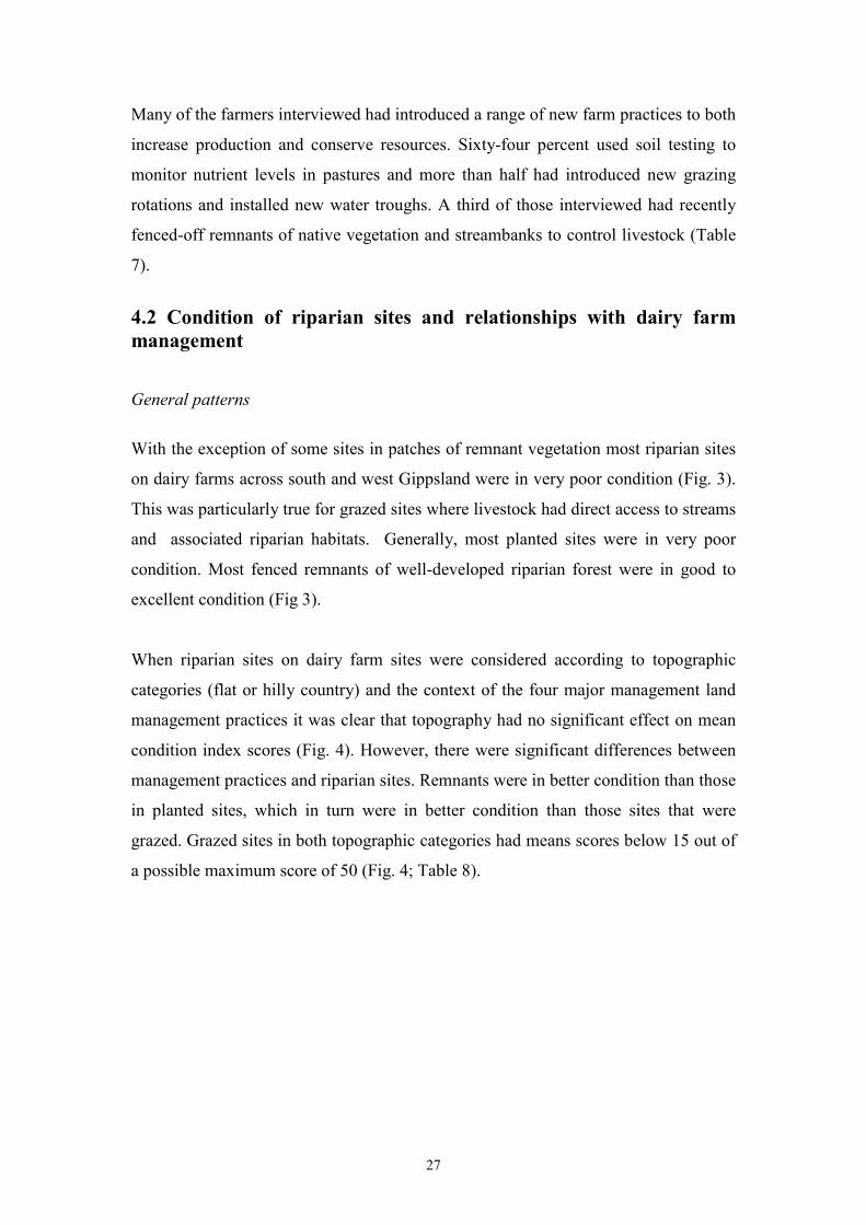
Many of the farmers interviewed had introduced a range of new farm practices to both
increase production and conserve resources. Sixty-four percent used soil testing to
monitor nutrient levels in pastures and more than half had introduced new grazing
rotations and installed new water troughs. A third of those interviewed had recently
fenced-off remnants of native vegetation and streambanks to control livestock (Table
7).
4.2 Condition of riparian sites and relationships with dairy farmmanagement
General patterns
With the exception of some sites in patches of remnant vegetation most riparian sites
on dairy farms across south and west Gippsland were in very poor condition (Fig. 3).
This was particularly true for grazed sites where livestock had direct access to streams
and associated riparian habitats. Generally, most planted sites were in very poor
condition. Most fenced remnants of well-developed riparian forest were in good to
excellent condition (Fig 3).
When riparian sites on dairy farm sites were considered according to topographic
categories (flat or hilly country) and the context of the four major management land
management practices it was clear that topography had no significant effect on mean
condition index scores (Fig. 4). However, there were significant differences between
management practices and riparian sites. Remnants were in better condition than those
in planted sites, which in turn were in better condition than those sites that were
grazed. Grazed sites in both topographic categories had means scores below 15 out of
a possible maximum score of 50 (Fig. 4; Table 8).

28
Figure 3. Frequency of condition index score categories for riparian sites subject todifferent management on dairy farms in south and west Gippsland. Data pooled overflat and hilly regions.
0
10
20
30
40
50
v. poor poor average good excellent
Condition category
fenced, not planted
grazed
planted
remnant
Freq
uenc
y

29
0
10
20
30
40
50
flat hilly
fenced, not planted
grazed
planted
remnant
Con
ditio
n
Figure 4. Mean (+ 95% CL) condition index scores for riparian sites subject to
30
different management on dairy farms in flat and hilly regions of west and southGippsland.
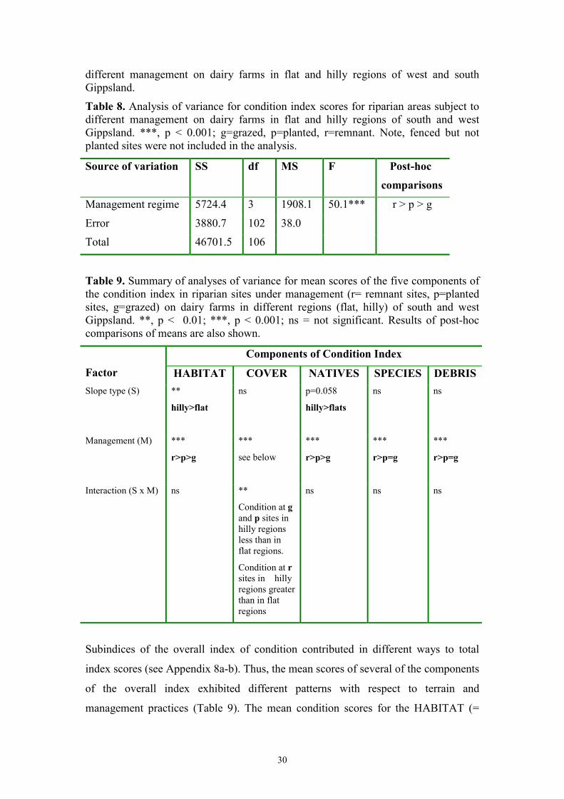
Table 8. Analysis of variance for condition index scores for riparian areas subject todifferent management on dairy farms in flat and hilly regions of south and westGippsland. ***, p < 0.001; g=grazed, p=planted, r=remnant. Note, fenced but notplanted sites were not included in the analysis.
Source of variation SS df MS F Post-hoc
comparisons
Management regime 5724.4 3 1908.1 50.1*** r > p > g
Error 3880.7 102 38.0
Total 46701.5 106
Table 9. Summary of analyses of variance for mean scores of the five components ofthe condition index in riparian sites under management (r= remnant sites, p=plantedsites, g=grazed) on dairy farms in different regions (flat, hilly) of south and westGippsland. **, p < 0.01; ***, p < 0.001; ns = not significant. Results of post-hoccomparisons of means are also shown.
Components of Condition Index
Factor HABITAT COVER NATIVES SPECIES DEBRISSlope type (S) **
hilly>flat
ns p=0.058
hilly>flats
ns ns
Management (M) ***
r>p>g
***
see below
***
r>p>g
***
r>p=g
***
r>p=g
Interaction (S x M) ns **
Condition at gand p sites inhilly regionsless than inflat regions.
Condition at rsites in hillyregions greaterthan in flatregions
ns ns ns
Subindices of the overall index of condition contributed in different ways to total
index scores (see Appendix 8a-b). Thus, the mean scores of several of the components
of the overall index exhibited different patterns with respect to terrain and
management practices (Table 9). The mean condition scores for the HABITAT (=

31
habitat continuity and extent) and NATIVE (=dominance of natives versus exotics)
components were significantly greater in hilly sites than in flat sites, while overall
mean scores were greater for remnants than replanted sites and those for replanted
sites were greater than for grazed sites. For COVER (=vegetation cover and
complexity) mean scores at grazed and replanted sites in hilly regions were less than
they were in flat regions, while remnant sites in hilly regions had greater mean scores
than those in flat regions. Mean scores for SPECIES (=indicative species) and
DEBRIS (=standing and fallen debris) components showed similar patterns to the
overall condition index (Tables 8 and 9).
For fenced and planted sites we wished to explore how long was required for riparian
condition to approach that of reference sites in the region (mean condition score for
the seven reference sites = 37). Our data (Fig. 5) indicates that there exists a strong
positive correlation between planting age and riparian condition scores, but that it
takes more than 16 years for planted sites to approach excellent condition (i.e. an
index score >40).
0
10
20
30
40
0 4 8 12 16
Con
ditio
n
Age in years
r33= 0.75, p< 0.001
Figure 5. Condition index scores for fenced and replanted riparian sites of differentage (since restoration) in flat and hilly regions of west and south Gippsland.
Relationships with other aspects of farms and their management
32
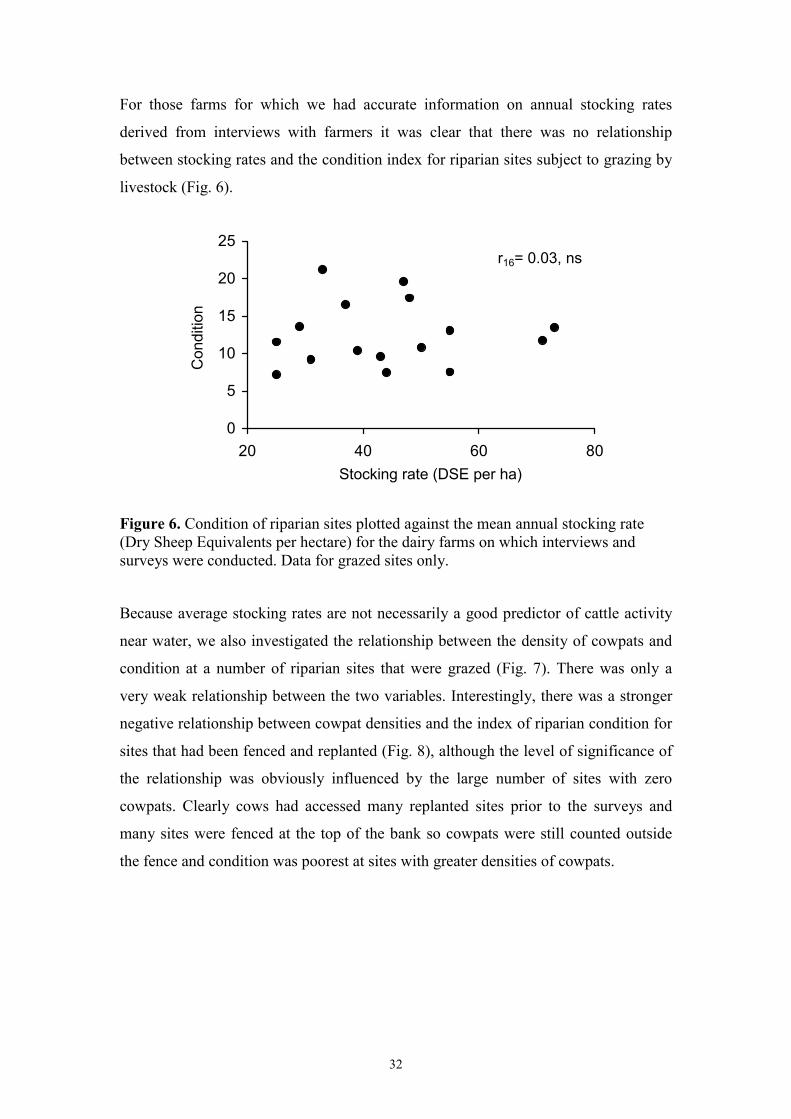
For those farms for which we had accurate information on annual stocking rates
derived from interviews with farmers it was clear that there was no relationship
between stocking rates and the condition index for riparian sites subject to grazing by
livestock (Fig. 6).
0
5
10
15
20
25
20 40 60 80
Con
ditio
n
Stocking rate (DSE per ha)
r16= 0.03, ns
Figure 6. Condition of riparian sites plotted against the mean annual stocking rate(Dry Sheep Equivalents per hectare) for the dairy farms on which interviews andsurveys were conducted. Data for grazed sites only.
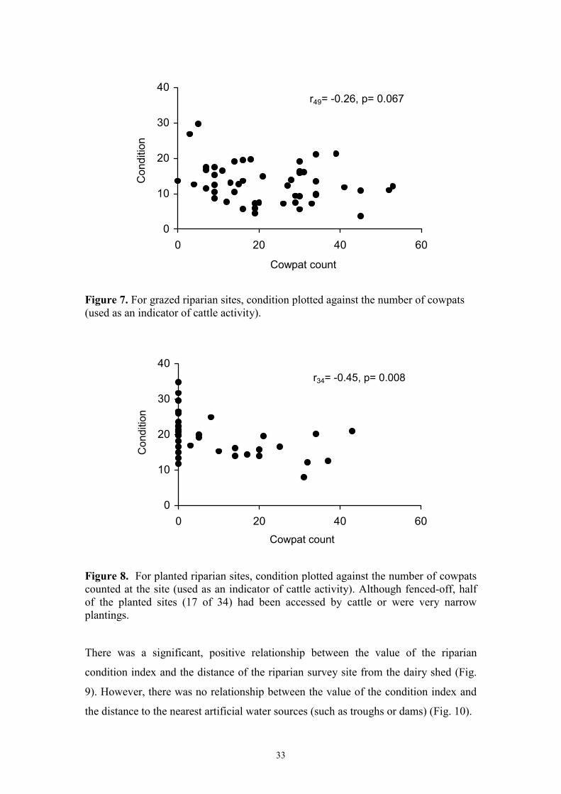
Because average stocking rates are not necessarily a good predictor of cattle activity
near water, we also investigated the relationship between the density of cowpats and
condition at a number of riparian sites that were grazed (Fig. 7). There was only a
very weak relationship between the two variables. Interestingly, there was a stronger
negative relationship between cowpat densities and the index of riparian condition for
sites that had been fenced and replanted (Fig. 8), although the level of significance of
the relationship was obviously influenced by the large number of sites with zero
cowpats. Clearly cows had accessed many replanted sites prior to the surveys and
many sites were fenced at the top of the bank so cowpats were still counted outside
the fence and condition was poorest at sites with greater densities of cowpats.
33
0
10
20
30
40
0 20 40 60
Con
ditio
n
Cowpat count
r49= -0.26, p= 0.067
Figure 7. For grazed riparian sites, condition plotted against the number of cowpats(used as an indicator of cattle activity).
0
10
20
30
40
0 20 40 60
Con
ditio
n
Cowpat count
r34= -0.45, p= 0.008
Figure 8. For planted riparian sites, condition plotted against the number of cowpatscounted at the site (used as an indicator of cattle activity). Although fenced-off, halfof the planted sites (17 of 34) had been accessed by cattle or were very narrowplantings.
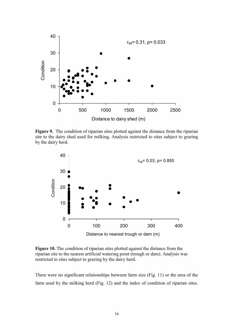
There was a significant, positive relationship between the value of the riparian
condition index and the distance of the riparian survey site from the dairy shed (Fig.
9). However, there was no relationship between the value of the condition index and
the distance to the nearest artificial water sources (such as troughs or dams) (Fig. 10).
34
Figure 9. The condition of riparian sites plotted against the distance from the ripariansite to the dairy shed used for milking. Analysis restricted to sites subject to grazingby the dairy herd.
0
10
20
30
40
0 100 200 300 400
Con
ditio
n
Distance to nearest trough or dam (m)
r48= 0.03, p= 0.855
Figure 10. The condition of riparian sites plotted against the distance from theriparian site to the nearest artificial watering point (trough or dam). Analysis wasrestricted to sites subject to grazing by the dairy herd.
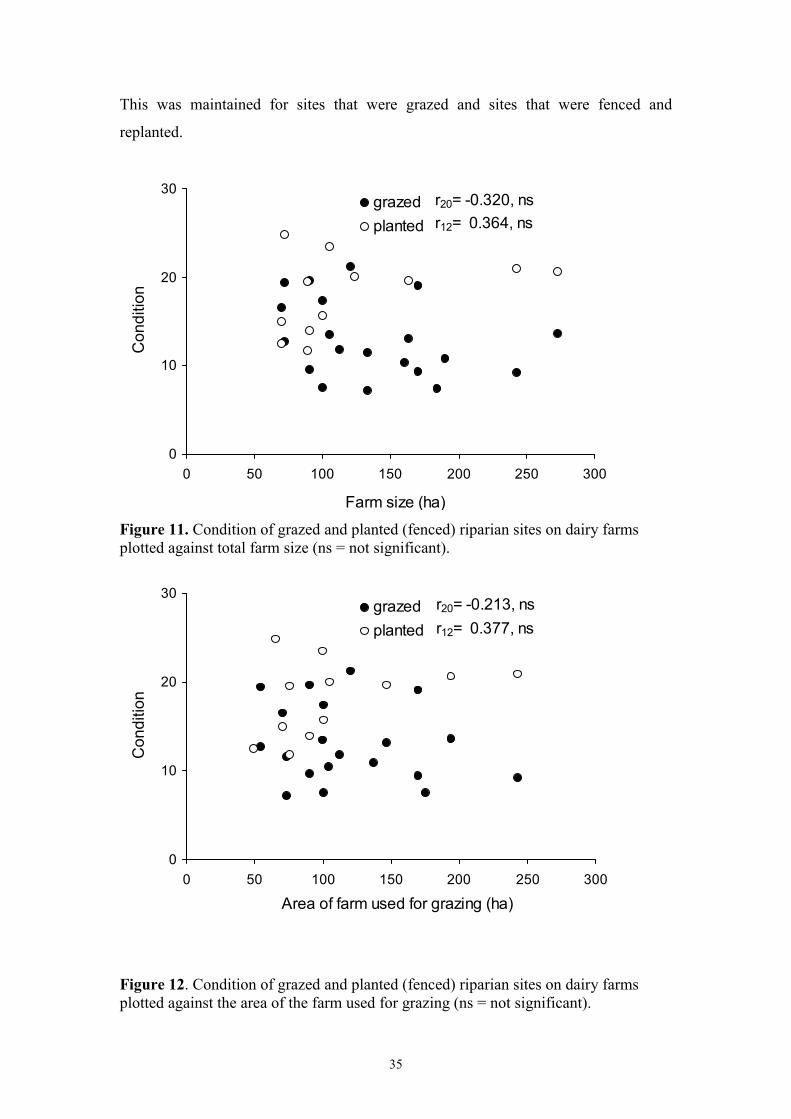
There were no significant relationships between farm size (Fig. 11) or the area of the
farm used by the milking herd (Fig. 12) and the index of condition of riparian sites.
0
10
20
30
40
0 500 1000 1500 2000 2500
Distance to dairy shed (m)
Con
ditio
nr49= 0.31, p= 0.033
35
This was maintained for sites that were grazed and sites that were fenced and
replanted.
Figure 11. Condition of grazed and planted (fenced) riparian sites on dairy farmsplotted against total farm size (ns = not significant).
Figure 12. Condition of grazed and planted (fenced) riparian sites on dairy farmsplotted against the area of the farm used for grazing (ns = not significant).
0
10
20
30
0 50 100 150 200 250 300
grazedplanted
Con
ditio
n
Farm size (ha)
r20= -0.320, nsr12= 0.364, ns
0
10
20
30
0 50 100 150 200 250 300
grazedplanted
Con
ditio
n
Area of farm used for grazing (ha)
r20= -0.213, nsr12= 0.377, ns
36
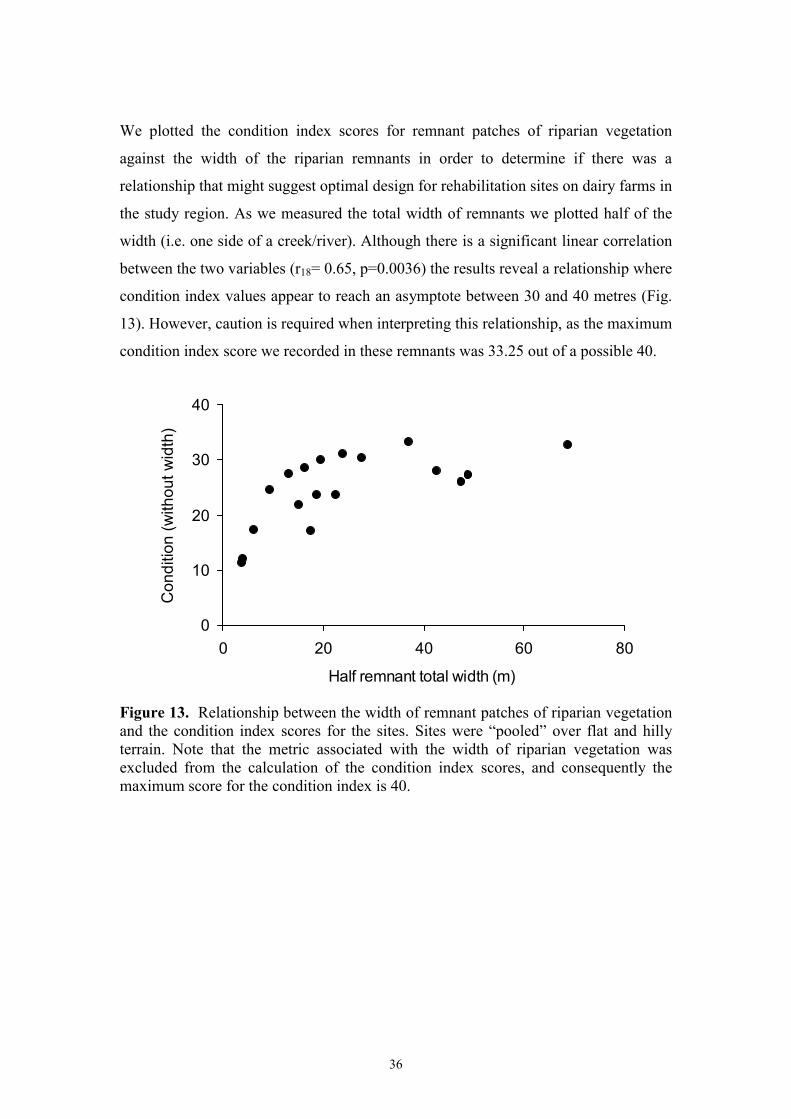
We plotted the condition index scores for remnant patches of riparian vegetation
against the width of the riparian remnants in order to determine if there was a
relationship that might suggest optimal design for rehabilitation sites on dairy farms in
the study region. As we measured the total width of remnants we plotted half of the
width (i.e. one side of a creek/river). Although there is a significant linear correlation
between the two variables (r18= 0.65, p=0.0036) the results reveal a relationship where
condition index values appear to reach an asymptote between 30 and 40 metres (Fig.
13). However, caution is required when interpreting this relationship, as the maximum
condition index score we recorded in these remnants was 33.25 out of a possible 40.
0
10
20
30
40
0 20 40 60 80
Con
ditio
n (w
ithou
t wid
th)
Half remnant total width (m)
Figure 13. Relationship between the width of remnant patches of riparian vegetationand the condition index scores for the sites. Sites were “pooled” over flat and hillyterrain. Note that the metric associated with the width of riparian vegetation wasexcluded from the calculation of the condition index scores, and consequently themaximum score for the condition index is 40.
37
5.0 DISCUSSION
5.1 Dairy farm management and riparian condition
The sizes, herd numbers and stocking rates of the 30 farms we visited for interviews
were typical of dairy farms in Gippsland (Australian Bureau of Statistics 1998) and
subsequently our findings are considered to be relevant across the region. Dairy farms
in Gippsland are intensive enterprises, and owing to the activities of cattle (Fleischner
1994; Trimble & Mendel 1995) one predictable outcome is degradation of riparian
habitats. Farms we visited for farmer interviews were typically small (most <200ha)
with stocking rates between 25-73 DSE.ha-1. In most cases farmers use all of their
properties for pasture production to support their herds. Despite finding that a
majority of farmers interviewed had some portion of their riparian areas fenced-off
from stock, most paddocks that contained streambank habitat were generally managed
in the same way as other paddocks, except when very wet, when farmers removed
stock.
Large amounts of waste from dairies and holding areas present a challenge for dairy
farmers. While most farmers interviewed had effluent ponds to manage waste, they
were not managed with any consistent practice, and some farmers allowed waste to
return directly to paddocks. Efficient effluent and fertiliser management is considered
critical to sustainable pasture and ecosystem management in dairy regions (Anon.
2001).
An important step in managing the disposal of concentrated waste from dairy
operations in a sustainable manner will be the maintenance of riparian strips to
minimise transport of nutrients to waterways. The efficacy of soils and riparian strips
to intercept phosphorus and other nutrients in the high rainfall, steep country typical
of parts of the Gippsland dairy region varies with soil type and other factors. Much of
the phosphorus mobilised during high rainfall events is in dissolved form which may
not be intercepted by riparian vegetation strips at some sites (Nash & Halliwell 1999,
Nash et al. 2000) but may be effectively trapped at others (Burkitt et al. 2001, Target
10 2002). Adoption of appropriate management strategies for the application of
phosphorus fertiliser promoted by extension programs include soil testing and
38
appropriate timing and siting of application (not near streams prior to predicted high
rainfall events) (e.g. Target 10 2002).
What was clear from interviews with dairy farmers was that due to the relatively small
size of dairy properties in the region, the trade situation has led to the necessity to
maintain high stocking rates. Consequently there is little ‘room to move’ for farmers
wishing to protect their riparian habitats. While many farmers in the region are using
fencing to exclude stock from streambank habitats, the most common reason given for
fencing was to prevent cattle having access to neighbouring paddocks (i.e. for stock
management purposes). Nevertheless, the very active Landcare groups in the region
attest to the number of dairy farmers with a motivation for fencing and replanting of
riparian habitats to conserve streambanks and associated biodiversity.
It is clear from our data that past and present management of the landscape for dairy
farming in south and west Gippsland has resulted in severe degradation of riparian
habitats. The severity of degradation was similar in the flat terrain of the Gippsland
Plain and hilly terrain of the Strezlecki Ranges. The riparian sites in ‘best’ condition
were in patches of fenced remnant riparian forest. However, even the remnants did
not receive maximum condition index scores owing to abundance of weeds, the lack
of vegetation complexity and only small amounts of organic debris (relative to
reference site conditions).
Riparian sites that had been fenced off and replanted (=planted sites in our results)
received relatively low condition index scores. Generally, this reflected the fact that
rehabilitation of these sites was recent and most sites only planted canopy-forming
species (i.e. no understorey). When we compared planted sites of different ages it was
clear that it takes more than 16 years for these planted sites to attain an excellent
condition index score.
Riparian sites in paddocks that are used for grazing of herds were generally in very
poor condition. Clearing of vegetation to create pastures, past grazing and present
intensive grazing practices with high stocking rates have resulted in riparian sites that
have little or no overstorey, abundance of exotic pasture grasses and little or no
terrestrial litter. There is consequently little or no shading of streams and little input of

39
terrestrial organic matter to streams, resulting in degraded in-stream habitat structure
and food web dynamics (Bunn et al. 1999, Robertson et al. 1999). There is also little
ground cover, coarse woody debris and leaf litter cover on the ground within riparian
vegetation thickets, decreasing local biodiversity.
What was clear from the information we collected was that, apart from fencing
riparian habitats from the activities of cattle, other recommended management
initiatives aimed at reducing the impacts of livestock on riparian zones will not be
effective in rehabilitating riparian habitats under the current stocking rates used on
Gippsland dairy farms. For instance, different rotations of stock in riparian paddocks
and the provision of off-stream watering points (LWRRDC 1996) are often effective
in protecting riparian habitats in drier regions where stocking rates are low (Elmore
1992, Jansen & Robertson 2001a, MacLeod 2002). However, for Gippsland dairy
farms we found no relationship between stocking rate and the index of riparian
condition. Although stocking rate is generally a poor predictor of the activities of
livestock on riparian habitats (Robertson 1997), with the small size of paddocks in
Gippsland dairy farms cattle are likely to exert similar pressure on all vegetation
within the paddock. It is thus not surprising that we observed only a very weak
relationship between cowpat counts (our index of cattle activity in the riparian zone)
and condition scores. This contrasted to our previous work in beef-grazing country on
the floodplain of the Murrumbidgee River in New South Wales, where cowpat counts
explained significant proportions of the variation in riparian condition index scores
and biodiversity responses in riparian habitats (Jansen & Robertson 2001a,b).
We also found no evidence that the positioning of alternative watering points resulted
in better condition index scores for riparian sites. In lower rainfall areas, where mean
annual stocking rates were generally <5 DSE.ha-1 and paddock sizes are much larger,
there is good evidence that the provision of off-stream watering points form part of
successful strategies to improve riparian condition (Jansen & Robertson 2001a,
Macleod 2002).
Interestingly we found a statistically significant correlation between distances of
riparian sites from dairy sheds and riparian condition index score for those sites. Since
our condition index was based on structural features that are used as proxy measures

40
of riparian function (Table 1), it is likely that a cause of such a relationship is
proximity to dairy sheds increases the likelihood of physical damage to riparian
vegetation by cattle. Gourley and Durling (2002) have reported that soil phosphorus
levels increase with proximity to dairy sheds in Gippsland, presumably as a result of
dairy cow waste being concentrated in these areas. This indicates both that most soils
are efficient traps for phosphorus and that placement of dairy sheds as far as possible
from streams will decrease the loss of nutrients to streams as well as physical damage
to riparian habitats.
One of the most vexing questions relating to the restoration of river/creek banks is
what width of riparian vegetation is required to maintain natural functions of riparian
systems. There is no simple answer to such a question, since riparian habitats support
a variety of ecosystem functions (Naiman & Decamps 1997). Within regions,
variation in each functional attribute can occur with position in catchment, soil type,
season and stream flow.
In this study when scores of riparian index condition were plotted against width of
riparian vegetation (for 18 sites that had intact remnants of riparian vegetation
communities) we found that condition values reached a plateau when vegetation was
30 metres wide on either side of a stream. Thus, it appears that such a width is
required in the Gippsland dairy region to obtain an excellent condition score.
5.2 Recommendations
We set out to explore relationships between the management of dairy farms and the
condition of riparian habitats across Gippsland, and consequently to identify possible
best management practices. These would be further investigated at demonstration
sites to be established on dairy farms. Our recommendations are not tempered by what
might be cost-effective, but rather what would be most beneficial from an ecological
point of view.
The following recommendations regarding best practice arise directly from the results
of this study.
41
� Rehabilitation of degraded riparian sites currently subject to direct access by dairy
cattle is best achieved by fencing-off riparian areas. Other recommended practices
such as the provision of off-stream watering points and ‘spelling’ of riparian
paddocks are not as effective on dairy farms in Gippsland given current stocking
rates.
� In order to restore riparian sites to near excellent condition (as measured by our
index of riparian condition) fenced riparian strips will need to be at least 30 metres
wide on either side of a stream or river.
� When siting new dairy sheds on farms, they should be as far away from streams as
possible.
42
REFERENCES
Anderson, M.J. (2001). A new method for non-parametric multivariate analysis ofvariance. Austral Ecology, 26, 32-46.
Anon. (n.d.) Strezlecki Web Page (online). http://members.dcsi.net.au/kimjulie/index.html [Accessed February 2003]
Anon. (2001) Sustaining our natural resources – Dairying for Tomorrow (online). http://www.dairyingfortomorrow.com/reports/reportpluscover.pdf. Principaleditor P. Day. The Dairy Research and Development Corporation. Melbourne,Victoria. [Accessed 17th April 2002].
Australian Bureau of Statistics (1998) The Victorian Dairy Industry. Year Book Australia. (online).
http://www.abs.gov.au/ausstats/[email protected]/94713ad445ff1425ca25682000192af2/995ba863e1a51443ca2569de0026c586!OpenDocument. [Accessed January2003]
Boulton, A. J. (1999) An overview of river health assessment: philosophies, practice,problems and prognosis. Freshwater Biology, 41, 469-479.
Bunn, S. E., Davies, P. M., & Mosisch, T. D. (1999) Ecosystem measures of riverhealth and their response to riparian and catchment degradation. FreshwaterBiology 41, 333-45.
Bureau of Meteorology (2003) Climate averages for Australian sites – Victoria(online). http://www.bom.gov.au/climate/averages/tables/ca_vic_names.shtml[Accessed February 2003]
Burkitt, L.L., Gourley, C.J.P., Sale P.W.G., Uren, N.C., & Hannah, M.C. (2001)Factors affecting the change in extractable phosphorus following theapplication of phosphatic fertiliser on pasture soils in southern Victoria.Australian Journal of Soil Research 39, 759-771.
Clarke, K.R. (1993). Non-parametric multivariate analyses of changes in communitystructure. Australian Journal of Ecology, 18, 117-143.
Clarke, K.R. & Warwick, R.M. (1994). Change in marine communities: an approachto statistical analysis and interpretation. Natural Environment Research
Council, U. K.
Curtis, A., Robertson, A., & Tennant, W. (2001) Understanding landholderwillingness and capacity to improve the management of river frontages in theGoulburn Broken Catchment. Johnstone Centre Report No. 157. TheJohnstone Centre, Charles Sturt University, Albury.
DPI (2002) Department of Primary Industries (online), http://www.nre.vic.gov.au [Accessed April 2002]
43
Elmore, W. (1992) Riparian responses to grazing practices. In: Watershed Management: Balancing Sustainability and Environmental Change (ed. R.J.Naiman), pp.442-457. Springer, New York, NY.
Fairweather, P. G. (1999) State of environment indicators of 'river health': exploringthe metaphor. Freshwater Biology, 41, 211-220.
Fleischner, T. L. (1994) Ecological costs of livestock grazing in western NorthAmerica. Biological Conservation, 8, 629-644.
GippsDairy. (2001) Regional Natural Resource Action Plan for the Gippsland Dairy Industry. Terry Makin & Associates. Viewbank, Victoria and NRM consultingBalaclava, Victoria.
Gourley, C. & Durling, P. (2002) Watch where you spread that fertiliser. AustralianDairyfarmer Magazine, March-April, 22-24.
Jansen, A., & Robertson, A. I. (2001a) Relationships between livestock managementand the ecological condition of riparian habitats along an Australian floodplainriver. Journal of Applied Ecology, 38, 63-75.
Jansen, A., & Robertson, A.I. (2001b) Riparian bird communities in relation to landmanagement practices in floodplain woodlands of south-eastern Australia.Biological Conservation, 100, 173-185.
Karr, J. R. (1999) Defining and measuring river health. Freshwater Biology, 41, 221-234.
Ladson, A. R., White, L. J., Doolan, J. A., Finlayson, B. L., Hart, B. T., Lake, S. &Tilleard, J. W. (1999) Development and testing of an Index of StreamCondition for waterway management in Australia. Freshwater Biology, 41,453-468.
LWRRDC (1996) Managing stock. Riparian management fact sheet 6. Land andWater Resources Research and Development Corporation, Canberra.
McLaren, C. (1997) Dry Sheep Equivalents for comparing different classes oflivestock (online).
http://www.nre.vic.gov.au/web/root/domino/infsheet.nsf/HTMLPages/NRE+Note+Series+Homepage?Open Agricultural Notes. Department of PrimaryIndustries, Victoria [Accessed 16th September 2002].
MacLeod, N. D. (2002) Watercourses and riparian areas. In: Managing andconserving grassy woodlands. Eds S. McIntyre, J.G. McIvor and K.M. Heard,CSIRO Publishing, Collingwood. pp 143-176.
Naiman, R. J. & Decamps, H. (1997) The ecology of interfaces: Riparian zones.Annual Review of Ecology and Systematics, 28, 621-658.

44
Nash, D.M., & Halliwell, D.J. (1999) Fertilisers and phosphorus loss from productivegrazing systems. Australian Journal of Soil Research 37, 403-429.
Nash, D.M., Hannah, M., Halliwell, D.J., & Murdoch, C. (2000) Factors affectingphosphorus export from a pasture-based grazing system. Journal ofEnvironmental Quality 29, 1160-1166.
RFA (1999) Regional Forest Agreements, Victoria (online),http://www.rfa.gov.au/rfa/vic/gipps/raa/biodiv/index.html [Accessed April2002].
Robertson, A. I. (1997) Land-water linkages in floodplain river systems: the influenceof domestic stock. Frontiers in Ecology: Building the Links (eds N. Klomp &I. Lunt), pp. 207-218. Elsevier Scientific, Oxford.
Robertson, A. I., Bunn, S. E., Boon. P.I., & Walker, K. F. (1999) Sources, sinks andtransformations of organic carbon in Australian floodplain rivers. Marine andFreshwater Research 50, 813-29.
Target 10 (2002) Fertilising dairy pastures. Target 10 Manuals, Resources (online),http://www.nre.vic.gov.au/web/root/domino/target10/t10frame.nsf/ [AccessedJanuary 2003]
Trimble, S. W. & Mendel, A. C. (1995) The cow as a geomorphic agent - A criticalreview. Geomorphology, 13, 233-253.
Waterwatch (2000) Waterwatch Victoria – West Gippsland (online)http://www.vic.waterwatch.org.au/contacts/wgipp.htm (Accessed February2003)

45
APPENDICIES
46
Appendix 1. (a) Ecological Vegetation Class (EVC) description and dominant species list for Gippsland Plain bioregion and Lowland Forest EVC. Allinformation from:
RFA (1999) Regional Forest Agreements, Victoria (online),http://www.rfa.gov.au/rfa/vic/gipps/raa/biodiv/index.html [Accessed April2002].
Gippsland Plains Lowland Forest is only recorded from the pre-1750 mappingproject. It would have occurred on the Tertiary and early Pleistocene terraces of thePerry land system, often in a mosaic with Damp Sands Herb-rich Woodland on theplains south and west of Moormung State Forest. This depleted floristic community isonly found today in a few road reserves in the area where it has been mapped asDepauperate Lowland Forest due to a high fire frequency over time resulting in a veryspecies depauperate understorey. Soils consist of aeolian and marine sands of lowdunes with a clay base which can be penetrated by shrub and tree roots. Elevation isin the range of 5 to 120m above sea level and annual average rainfall is approximately550-700 mm.
This floristic community would have had an overstorey dominated by WhiteStringybark Eucalyptus globoidea and But But E. bridgesiana with a denseunderstorey of smaller trees and shrubs including Blackwood Acacia melanoxylon,Lightwood A. implexa, Silver Wattle A. dealbata, Spike Wattle A. oxycedrus, ShinyCassinia Cassinia longifolia, Hop Bitter-pea Daviesia latifolia, Burgan Kunzeaericoides, Silver Banksia Banksia marginata (tree-form), Purple Coral-peaHardenbergia violacea and Smooth Parrot-pea Dillwynia glaberrima. A dense groundcover of bracken, grasses and forbs would have included Austral Bracken Pteridiumesculentum, Grey Tussock-grass Poa sieberiana, Kangaroo Grass Themeda triandra,Weeping Grass Microlaena stipoides, Common Raspwort Gonocarpus tetragynus,Germander Raspwort G. teucrioides, Small Poranthera Poranthera microphylla,Common Lagenifera Lagenifera stipitata and Glycine spp. Thatch Saw-sedge Gahniaradula, Spiny-headed Mat-rush Lomandra longifolia and Wattle Mat-rush L.filiformis would also have been present.
Latrobe Valley Lowland Forest is found across the Gippsland plains but includesareas south of Traralgon at Gormandale. It grows on loose, light-grey to white sandytopsoil over a cemented gravel, clay or sand subsoil. The sandy topsoil promotes theoccurrence of various healthy understorey species that reflects a floristic associationwith Heathy Woodland. Average annual rainfall is 800-900 mm and elevation is 180-220m above sea level.
The overstorey is usually dominated by Yertchuk E. consideniana, Narrow-leafPeppermint E.radiata but E. obliqua and E. viminalis ssp. pryoriana may also bepresent. Species in the shrub layer include Sunshine Wattle Acacia terminalis, BurganKunzea ericoides, Showy Bossiaea Bossiaea cinerea, Prickly Tea-tree Leptospermumcontinentale, Common Heath Epacris impressa, Snow Daisy-bush Olearia lirata,Broom Spurge Amperea xiphoclada and scattered Saw Banksia Banksia serrata.
47
The ground layer includes dense Austral Bracken Pteridium esculentum in addition toCommon Raspwort, Gonocarpos tetragynus, Thatch Saw-sedge Gahnia radula andTussock-grass Poa sp.
Appendix 1. (b) Ecological Vegetation Class (EVC) description and dominant species list for Strezlecki Ranges bioregion and Damp Forest EVC.
Damp Forest is widespread in Gippsland in moderately fertile areas between WetForest, the drier end of Shrubby Foothill Forest and the driest forest types such asLowland Forest, Herb-rich Foothill Forest, and Heathy Woodland. It develops on thedrier sites in Wet Forest or on the margins of Warm Temperate Rainforest. It alsooccurs on protected slopes associated with Tussocky Herb-rich Foothill Forest,Lowland Forest or even Heathy Woodland, provided topographic protection issufficient.
In the lowlands and dissected country below 700m Damp Forest favours gullies oreastern and southern slopes. Above this elevation and in higher rainfall zones theeffect of cloud cover at ground level and the subsequent fog drip permits this class toexpand out of the gullies onto broad ridges and northern and western aspects. Itoccurs on a wide range of geologies and soils are usually colluvial, deep and well-structured with moderate to high levels of humus in the upper soil horizons(Woodgate et al. 1994). Rainfall is approximately 800-1600 mm per annum andelevation ranges from sea level in South Gippsland to up to 1000m in the montaneareas where it merges into Montane Damp Forest.
The dominant eucalypts are commonly Messmate Eucalyptus obliqua and MountainGrey Gum E. cypellocarpa. A range of other species may be present as well such asYellow Stringybark E.muelleriana (in South Gippsland with Sticky Wattle Acaciahowittii present in the understorey), Silvertop E.sieberi, Gippsland Blue Gum E.globulus ssp. pseudoglobulus, Narrow-leaf Peppermint E.radiata, GippslandPeppermint E. croajingolensis, Brown Stringybark E. baxteri and Swamp Gum E.ovata in the vicinity of poorer drainage. Trees of Blackwood Acacia melanoxylon andSilver Wattle Acacia dealbata are often present.
The understorey typically includes moisture-dependent fern species such as CommonGround-fern Calochlaena dubia, Gristle Fern Blechnum cartilagineum, MotherShield-fern Polystichum proliferum and Rough Tree-fern Cyathea australis, and thepresence of broad-leaved species typical of wet forest mixed with elements from dryforest types such as Lowland Forest.
Broad-leaved species include Hazel Pomaderris Pomaderris aspera, VictorianChristmas-bush Prostanthera lasianthos, Snow Daisy-bush Olearia lirata, Cassiniaspp, Hop Goodenia Goodenia ovata, Elderberry Panax Polyscias sambucifolia andWhite Elderberry Sambucus gaudichaudiana. Sweet Pittosporum Pittosporumundulatum is often present in South Gippsland. The wet forest shrub, Prickly Currant-bush Coprosma quadrifida, and Fireweed Groundsel Senecio linearifolius are alsocommon. Drier shrubby elements include Prickly Moses Acacia verticillata, PricklyBush Pea Pultenaea juniperina, Narrow-leaf Wattle Acacia mucronata and VarnishWattle Acacia verniciflua. Other species commonly present are Austral Bracken
48
Pteridium esculentum and Forest Wire-grass Tetrarrhena juncea, Broad-leafStinkweed Opercularia ovata, Tall Sword-sedge Lepidosperma elatius, Wonga VinePandorea pandorana and Mountain Clematis Clematis aristata.
At the drier end of Damp Forest a number of species start to appear such as Narrow-leaf Peppermint Eucalyptus radiata, Narrow-leaf Wattle Acacia mucronata, CherryBallart Exocarpos cupressiformis, Grey Tussock-grass Poa sieberiana, Prickly Tea-tree Leptospermum continentale and Thatch Saw-sedge Gahnia radula. At WilsonsPromontory, the shrub Blue Olive-berry Elaeocarpus reticulatus is a common specieswhich indicates its close affinities with Wilson’s Promontory Overlap WarmTemperate Rainforest.
Riparian habitats in Damp Forest contain indicator species of Riparian Forest such asSoft Water-fern Blechnum minus, Fishbone Water-fern Blechnum nudum, AustralKing-fern Todea barbara, Scrambling Coral-fern Gleichenia microphylla, Tall Saw-sedge Gahnia clarkei and Tall Sedge Carex appressa.
Appendix 1. (c) Ecological Vegetation Class (EVC) description and dominant species list for Strezlecki Ranges bioregion and Wet Forest EVC.
This EVC includes a very wide range of structural variation ranging from tall old-growth forest up to 60m in height through to regrowth forest and scrub which has thepotential to support tall forest. It also includes treeless areas dominated by wet scruband even “oldfields” which were once cleared but are now dominated by nativevegetation.
Wet Forest is dominated by Mountain Ash Eucalyptus regnans but may be dominatedlocally by Blackwood Acacia melanoxylon or Silver Wattle A. dealbata. A range ofother eucalypt species can be present but these tend to be on the periphery ofextensive areas dominated by Mountain Ash E. regnans. These include Manna GumE. viminalis (often occurring along major river flats and on associated slopes),Strzelecki Gum Eucalyptus strzeleckii, Gippsland Blue Gum E. globulus ssp.pseudoglobulus, Messmate E. obliqua, and Mountain Grey Gum E. cypellocarpawhich occurs on the edges of Wet Forest stronghold areas immediately before DampForest becomes more developed. Tree-ferns are sometimes present, particularlyRough Tree-fern Cyathea australis on the slopes and Soft Tree-fern Dicksoniaantarctica along the creek lines as well as some of the “wet-ferns” such as MotherShield-fern Polystichum proliferum and Hard Water-fern Blechnum wattsii. Common understorey species are the broad-leaved shrubs such as Snow Daisy-bushOlearia lirata, Musk Daisy-bush O. argophylla, Blanket Leaf Bedfordia arborescens,Hazel Pomaderris Pomaderris aspera, Cassinia spp., Tree Lomatia Lomatia fraseriand Austral Mulberry Hedycarya angustifolia. The prickly shrub, Prickly Currant-bush Coprosma quadrifida, and the vines Mountain Clematis Clematis aristata andWonga Vine Pandorea pandorana are also often present. Other shrubs sometimesinclude Sweet Pittosporum Pittosporum undulatum, Tree Lomatia Lomatia fraseri andVictorian Christmas-bush Prostanthera lasianthos. At the drier end of this group theunderstorey becomes very low in stature (less than 2m) and broad-leaved species
49
other than Snow Daisy-bush Olearia lirata are notably absent. This variant tends tooccur on the most exposed, drier northerly aspects.
Wet Forest develops extensively around the localised areas of Cool TemperateRainforest in the study area. At the dry end of its range it changes to Damp Forestand Shrubby Foothill Forest, which tends to first appear on the drier, steeper aspectsassociated with Wet Forest in the more protected sites.
There are two floristic communities of Wet Forest: Gippsland 1 Wet Forest andGippsland 2 Wet Forest.
Floristic Community: Gippsland 1 Wet ForestGippsland 1 Wet Forest occurs across the study area along creeks and on south-facingslopes and gullies. It grows on a variety of geologies, which combine with highrainfall and moist loamy organic soils to provide a fertile environment for tall trees,broad-leaf shrubs and ferns. Average rainfall is high ranging from 700–1200mm,with high effective rainfall on protected southerly slopes. It grows at a range ofaltitudes from 500-1100m above sea level.
The overstorey may carry a range of eucalypts including Messmate StringybarkEucalyptus obliqua, Gippsland Peppermint Eucalyptus croajingolensis, Narrow-leafPeppermint E. radiata in the west of the study area and E. croajingolensis to the eastof the study area. Manna Gum Eucalyptus viminalis and E. obliqua may co-dominante in some areas
Silver Wattle Acacia dealbata is the ubiquitous understorey tree in this EVC. Adiversity of tall broad-leaved shrubs are prominent and often form a complete cover,although this may be broken by an equally dense layer of tree ferns. The mostcommon tall shrubs include Hazel Pomaderris Pomaderris aspera, Blanket LeafBedfordia arborescens, Musk Daisy-bush Olearia argophylla, and Rough CoprosmaCoprosma hirtella. Common Cassinia Cassinia aculeata, Prickly Currant-bushCoprosma quadrifida, Elderberry Panax Polyscias sambucifolia, Snow Daisy-bushOlearia lirata and Dusty Daisy-bush O. phlogopappa form a shorter layer beneath thetaller shrub layer.
Tree ferns are often present with Soft Tree-fern Dicksonia antarctica at the wettestsites and Rough Tree-fern Cyathea australis at lower elevations and on slightly driersites. Ground ferns include Austral Bracken Pteridium esculentum, Mother Shield-fern Polystichum proliferum and Fishbone Water-fern Blechnum nudum.
The ground layer is equally rich in species, dominated by large moisture-loving herbs,and graminoids such as the large tussocks of Tasman Flax-lily Dianella tasmanica,Tussock-grasses Poa spp. and Tall-headed Mat-rush Lomandra longifolia. Thediverse array of smaller forbs include Ivy-leaf Violet Viola hederacea, Soft CranesbillGeranium potentilloides, Bidgee Widgee Acaena novae-zelandiae, Hairy PennywortHydrocotyle hirta and Common Lagenifera Lagenifera stipitata. Forbs indicative ofWet Forest include Mountain Cotula Leptinella filicula, Scrub Nettle Urtica incisaand Forest Starwort Stellaria flaccida.
Floristic Community:Gippsland 2 Wet Forest
50
Gippsland 2 Wet Forest grows in similar environments to Gippsland 1 Wet Forest.Rainfall is very high, ranging from 950–1350mm per annum and effective rainfallextremely high. It ranges in elevation from 700 to 1160m above sea level, thusreaching montane environments.
Gippsland 2 Wet Forest is the wettest of the eucalypt-dominated vegetation types. Athigher elevations Alpine Ash Eucalyptus delegatensis dominates the overstorey whilstat lower elevations Mountain Ash E. regnans dominates wetter sites and Manna GumEucalyptus viminalis and species of the narrow-leaved peppermint group areprominent (for example, Narrow-leaved Peppermint Eucalyptus radiata s.s., MonaroPeppermint Eucalyptus radiata ssp. robertsonii and Gippsland Peppermint Eucalyptuscroajingolensis). The understorey tree layer is well developed with Silver WattleAcacia dealbata and Blackwood A. melanoxylon dominating.
The shrub layer is usually very dense and may form an almost impenetrable thicket,especially after disturbance. It is most often dominated by Soft Tree-fern Dicksoniaantarctica and a mixture of large mesic shrubs including Banyalla Pittosporumbicolor, Mountain Tea-tree Leptospermum grandifolium, Blanket-leaf Bedfordiaarborescens, Victorian Christmas Bush Prostanthera lasianthos, Mountain PepperTasmannia lanceolata, Hazel Pomaderris Pomaderris aspera and Musk Daisy-bushOlearia argophylla. Several smaller shrubs are also common including CommonCassinia Cassinia aculeata, Elderberry Panax Polyscias sambucifolia, WhiteElderberry Sambucus gaudichaudiana and Dusty Daisy-bush Olearia phlogopappa..
The ground layer is also very dense and is dominated by ferns. Mother Shield-fernPolystichum proliferum, Fishbone Water-fern Blechnum nudum, Hard Water-fern B.wattsii, Ray Water-fern B. fluviatile and Austral Bracken Pteridium esculentumcommonly form a complete cover.
Common herbs and graminoids including Tussock-grasses Poa spp, Scrub NettleUrtica incisa, Shade Nettle Australina pusilla and Bidgee Widgee Acaena novae-zelandiae may reach high densities in open patches, often created by localdisturbance, or where the substrate is rocky. Other herbs and graminoids include TallSedge Carex appressa, Tasman Flax-lily Dianella tasmanica, Small-leaf BrambleRubus parvifolius, Hairy Pennywort Hydrocotyle hirta, Ivy-leaf Violet Violahederacea, Mountain Cotula Leptinella filicula, Forest Mint Mentha laxiflora andForest Starwort Stellaria flaccida. Forest Wire-grass Tetrarrhena juncea is alsocommon.
Vines are particularly rich in this community of Damp Forest. Mountain ClematisClematis aristata is most common with Common Apple-berry Billardiera scandens,Love Creeper Comesperma volubile, Austral Sarsaparilla Smilax australis, WombatBerry Eustrephus latifolius and Wonga Vine Pandorea pandorana often present.Climbers and scramblers are very prominent and the presence of Wombat BerryEustrephus latifolia and Austral Sarsaparilla Smilax australis emphasises floristiclinks for Warm Temperate Rainforest.
51
Appendix 1. (d) Ecological Vegetation Class (EVC) description and dominant species list for Strezlecki Ranges bioregion and Shrubby Foothill Forest EVC.
Strzelecki’s Shrubby Foothill Forest is found mainly on the northern and westernaspects of the higher slopes of the Strezlecki Ranges. It occurs in habitats at the drierend of Damp Forest extending from Carrajung on the eastern flank of the Strzelecki’sto Loch in the west. Soils are fertile, well-drained, grey-brown loams and clay loamsof Cretaceous origin. This EVC has been even more extensively cleared than WetForest in the Strzelecki’s with some of the few remaining intact remnant patchesbeing found at the Karl Harmann Reserve north-east of Leongatha and at Dickies Hillnear Mirboo North. It is floristically and geographically closely associated withHerb-rich Foothill Forest. Elevation ranges from 100-500m above sea level andaverage annual rainfall is 900-1100 mm.
The overstorey is dominated by Narrow-leaf Peppermint Eucalyptus radiata,Messmate E. obliqua, Mountain Grey Gum E. cypellocarpa and to a lesser extentSilver-top E. sieberi. A diverse, shrubby understorey characterises this EVC with alimited range of herbs and grasses in the ground layer.
Characteristic shrubs include Narrow-leaf Wattle Acacia mucronata, Dusty MillerSpyridium parvifolium, Prickly Currant-bush Coprosma quadrifida, Hazel PomaderrisPomaderris aspera, Snow Daisy-bush Olearia lirata, Shiny Cassinia Cassinialongifolia, Hop Goodenia Goodenia ovata, Handsome Flat-pea Platylobium formosumand Wiry Bauera Bauera rubioides.
The ground layer is very species poor and helps distinguish this EVC from Herb-richFoothill Forest. It includes Ivy-leaf Violet Viola hederacea, Forest Wire-grassTetrarrhena juncea, Austral Bracken Pteridium esculentum and Tall Sword-sedgeLepidosperma elatius.

52
Appendix 2. Interview sheet used by the interviewer for on-farm management practices on dairy farms in west and south Gippsland
LANDHOLDER INTERVIEW – On-farm Management(For interviewer’s use only)
Points to remember to tell farmer:� What project is about� What is riparian area in simple terms� All information completely confidential, names not used in reports
(and you will be provided with a copy of the reports)� Do you mind of I take photos of your creek for my future reference
(your name will not be placed with the photograph)?� I am going to ask you questions about: stocking rates and management
as well as streambank management (inform of what questions are coming using subheadings)
Owner/Manager: Interview Date:Property Name: Location:Interviewees: Ph. Number:Mailing Address: Creek Name:
General Questions� How big is your property?
______Hectares/acres� How long have you owned/managed this property?
______Months/years� Is this a family property (passed down through generations)?
YES/NO� If YES, for how long has it been in the family?
______Years� Has the property always operated as a dairy farm?
YES/NO� If NO, what is the farm’s history (if known)?
Stocking Rates and Paddock Sizes� What is the annual total stocking rate on your property?
______Total or Cow/Ha� Do your stocking rates vary by large numbers throughout the year (with seasons)?
YES/NO � If YES, by how many does it vary through the year (give a number or %)?
______No. or %� Has your farm ever carried more stock than the annual stocking rate in the past?
YES/NO� If YES, what was the maximum number it ran in the past?
______Total or Cow/Ha

53
� Of the current amount, how many cows constitute: � Milking herd? ______� Heifers? ______� Dry cows? ______� Calves? ______� Beef herd? ______
� What approximate % maximum area of the farm do the milking herd occupythroughout the year?
______% area� How many paddocks are there on your property?
______No. Paddocks� What is the average size of your paddocks
______Avg.� How many of your paddocks have rivers/creeks running through them
______No. Paddocks� What rotational grazing practices do you employ for your milking herd?
Day v.’s night �
12 hour �
24 hour �
Other � please specify
� Is the on/off grazing procedure on wet paddocks familiar to you? YES/NO
� If YES, how often do you employ this method of grazing?Regularly �
As needed �
Streambanks and watering points� Is there more than one river/creek running through your property (if so how
many)?YES/NO______No. Rivers/creeks
� Are the rivers/creeks on your property the main watering point for your stock YES/NO
� If NO, on average, how far are the watering points from the streambanks?______Metres
� Does flooding ever affect the movement/rotation of stock by loss of paddock use?
YES/NO� If YES, how often does this usually occur and for what length of time (duration)?
______How often______Length of time
� If flooding occurs, how far out of the creek channel do waters usually spread?______Metres
� How far are your dairy sheds located from your closest river/creek frontage?

54
______Meters
� Do you graze your river/creek frontage paddocks continuously or on a rotationalbasis?
Continuous/rotation� Approximately how many metres/kilometres of your land have river/creek
frontage?______Metres/Kilometres
� Have any areas of your river/creek frontage been fenced to exclude livestock? YES/NO
� If YES, what was your primary reason for fencing off your river/creek frontage?Prevent stock loss �
Improve condition/health of waterway/water quality �
Prevent stock accessing neighboring paddocks �
Prevent banks destabilizing �
Increase presence of flora and fauna species �
Better Stock Management �
Other (please specify) �
� Approximately how many metres/kilometres have been fenced? _____Metres/kilometres
� How long has this areas(s) been fenced off for? ______Months/Years
� Have you planted the fenced area with trees or understorey in any way?YES/NO
� What methods of weed management (if any) do you employ in these fencedwaterway areas?
Mechanical (hand removal) �
Spot spraying �
Broad herbicide treatment �
Crash grazing �
No treatment �
Other � please specify
� Do you allow stock into these fenced areas for any period of time? YES/NO
� What do you think is the ideal fencing width of waterways?______Width
Effluent, Irrigation and Stock Loss� Are any irrigation methods employed on your property?
YES/NO

55
� If YES, on average how often is irrigation used?Daily �
Weekly �
Monthly �
2-3 time per year �
As needed �
Other � please specify
� What is your primary method of irrigation?Spray irrigation �
Flood irrigation �
Lateral sprinkler �
Other � please specify
� Do you apply fertilisers to your river/creek frontage paddocks?YES/NO
� Do you use your dairy shed effluent on river/creek frontage paddocks forirrigation purposes?
YES/NO� What best describes your current dairy effluent system?
Single pond �
Two pond system �
Direct to pasture �
No system �
Other � please specify� Are you happy with your current dairy effluent system?
YES/NO� Would you like to change your current management of dairy shed effluent in the
future?YES/NO
� If YES, what would you like to do in the future?
� How often are your dairy effluent systems usually drained and/or cleaned?Daily �
Weekly �
2-3 times per year �
Once yearly �
Less than annually �� If you fenced off the stream banks on your farm would this reduce your time
needed for stock surveillance and stock mustering?YES/NO

56
� If YES, how much time would you save in an average week on the farm?______Hours/Mins
� What is the estimate of cow deaths on your farm each year in the following threewater associated areas:
Creeks and rivers �
Dams and swamps �
Erosion gullies and tunnels �
Conservation and New Management Regimes
� What new land management practices has your farm adopted recently that hasresulted in an improvement in the farm environment?
Fencing remnants �
Fencing rivers/creeks/drainage areas �
Tree planting �
Grazing techniques �
Fertiliser plans/soil tests �
Other (please specify) �
� What has been the effect of this new land management practice?
� Do you think these new land management practices were:Cost positive �
Cost negative �
Cost neutral �� Is there a Landcare group in your local area?
YES/NO� If YES, are you a member of the Landcare group in you area and which one is
this?YES/NO Group? ____________________
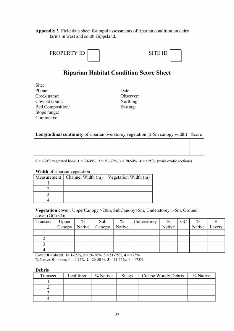
57
Appendix 3. Field data sheet for rapid assessments of riparian condition on dairy farms in west and south Gippsland.
PROPERTY ID SITE ID
Riparian Habitat Condition Score Sheet
Site:Phone: Date:Creek name: Observer:Cowpat count: Northing:Bed Composition: Easting:Slope range:Comments:
Longitudinal continuity of riparian overstorey vegetation (� 5m canopy width) Score
0 = <30% vegetated bank, 1 = 30-49%, 2 = 50-69%, 3 = 70-94%, 4 = >95% (mark exotic sections)
Width of riparian vegetation Measurement Channel Width (m) Vegetation Width (m)
1234
Vegetation cover: UpperCanopy >20m, SubCanopy>5m, Understorey 1-5m, Groundcover (GC) <1mTransect Upper
Canopy%
NativeSub
Canopy%
NativeUnderstorey %
NativeGC %
Native#
Layers1234
Cover: 0 = absent, 1= 1-25%, 2 = 26-50%, 3 = 51-75%, 4 = >75%% Native: 0 = none, 1 = 1-25%, 2 =26-50 %, 3 = 51-75%, 4 = >75%
DebrisTransect Leaf litter % Native Snags Coarse Woody Debris % Native
1234
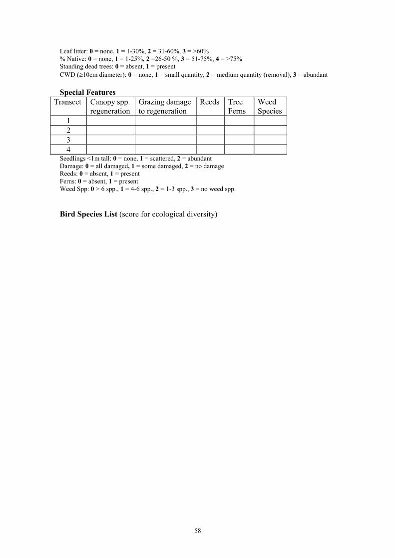
58
Leaf litter: 0 = none, 1 = 1-30%, 2 = 31-60%, 3 = >60%% Native: 0 = none, 1 = 1-25%, 2 =26-50 %, 3 = 51-75%, 4 = >75%Standing dead trees: 0 = absent, 1 = presentCWD (�10cm diameter): 0 = none, 1 = small quantity, 2 = medium quantity (removal), 3 = abundant
Special FeaturesTransect Canopy spp.
regenerationGrazing damageto regeneration
Reeds TreeFerns
WeedSpecies
1234
Seedlings <1m tall: 0 = none, 1 = scattered, 2 = abundantDamage: 0 = all damaged, 1 = some damaged, 2 = no damageReeds: 0 = absent, 1 = presentFerns: 0 = absent, 1 = presentWeed Spp: 0 > 6 spp., 1 = 4-6 spp., 2 = 1-3 spp., 3 = no weed spp.
Bird Species List (score for ecological diversity)
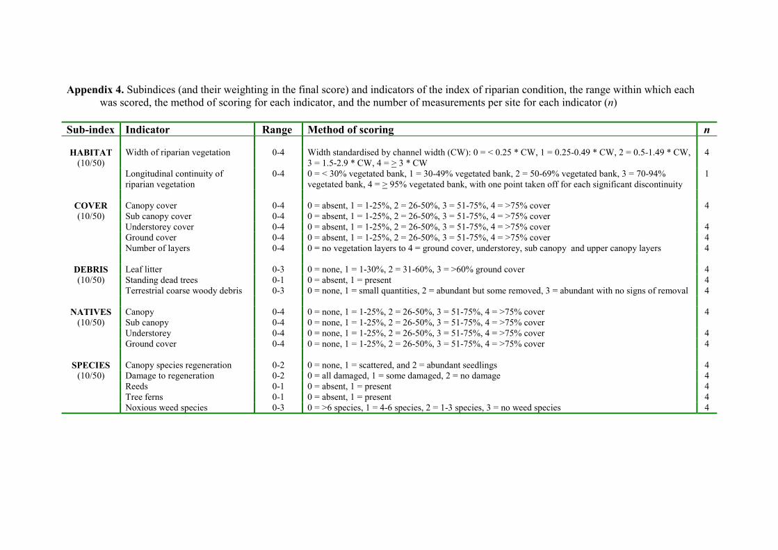
Appendix 4. Subindices (and their weighting in the final score) and indicators of the index of riparian condition, the range within which each was scored, the method of scoring for each indicator, and the number of measurements per site for each indicator (n)
Sub-index Indicator Range Method of scoring n
HABITAT(10/50)
Width of riparian vegetation 0-4 Width standardised by channel width (CW): 0 = < 0.25 * CW, 1 = 0.25-0.49 * CW, 2 = 0.5-1.49 * CW,3 = 1.5-2.9 * CW, 4 = > 3 * CW
4
Longitudinal continuity ofriparian vegetation
0-4 0 = < 30% vegetated bank, 1 = 30-49% vegetated bank, 2 = 50-69% vegetated bank, 3 = 70-94%vegetated bank, 4 = > 95% vegetated bank, with one point taken off for each significant discontinuity
1
COVER Canopy cover 0-4 0 = absent, 1 = 1-25%, 2 = 26-50%, 3 = 51-75%, 4 = >75% cover 4(10/50) Sub canopy cover 0-4 0 = absent, 1 = 1-25%, 2 = 26-50%, 3 = 51-75%, 4 = >75% cover
Understorey cover 0-4 0 = absent, 1 = 1-25%, 2 = 26-50%, 3 = 51-75%, 4 = >75% cover 4Ground cover 0-4 0 = absent, 1 = 1-25%, 2 = 26-50%, 3 = 51-75%, 4 = >75% cover 4Number of layers 0-4 0 = no vegetation layers to 4 = ground cover, understorey, sub canopy and upper canopy layers 4
DEBRIS Leaf litter 0-3 0 = none, 1 = 1-30%, 2 = 31-60%, 3 = >60% ground cover 4(10/50) Standing dead trees 0-1 0 = absent, 1 = present 4
Terrestrial coarse woody debris 0-3 0 = none, 1 = small quantities, 2 = abundant but some removed, 3 = abundant with no signs of removal 4
NATIVES Canopy 0-4 0 = none, 1 = 1-25%, 2 = 26-50%, 3 = 51-75%, 4 = >75% cover 4(10/50) Sub canopy 0-4 0 = none, 1 = 1-25%, 2 = 26-50%, 3 = 51-75%, 4 = >75% cover
Understorey 0-4 0 = none, 1 = 1-25%, 2 = 26-50%, 3 = 51-75%, 4 = >75% cover 4Ground cover 0-4 0 = none, 1 = 1-25%, 2 = 26-50%, 3 = 51-75%, 4 = >75% cover 4
SPECIES Canopy species regeneration 0-2 0 = none, 1 = scattered, and 2 = abundant seedlings 4(10/50) Damage to regeneration 0-2 0 = all damaged, 1 = some damaged, 2 = no damage 4
Reeds 0-1 0 = absent, 1 = present 4Tree ferns 0-1 0 = absent, 1 = present 4Noxious weed species 0-3 0 = >6 species, 1 = 4-6 species, 2 = 1-3 species, 3 = no weed species 4
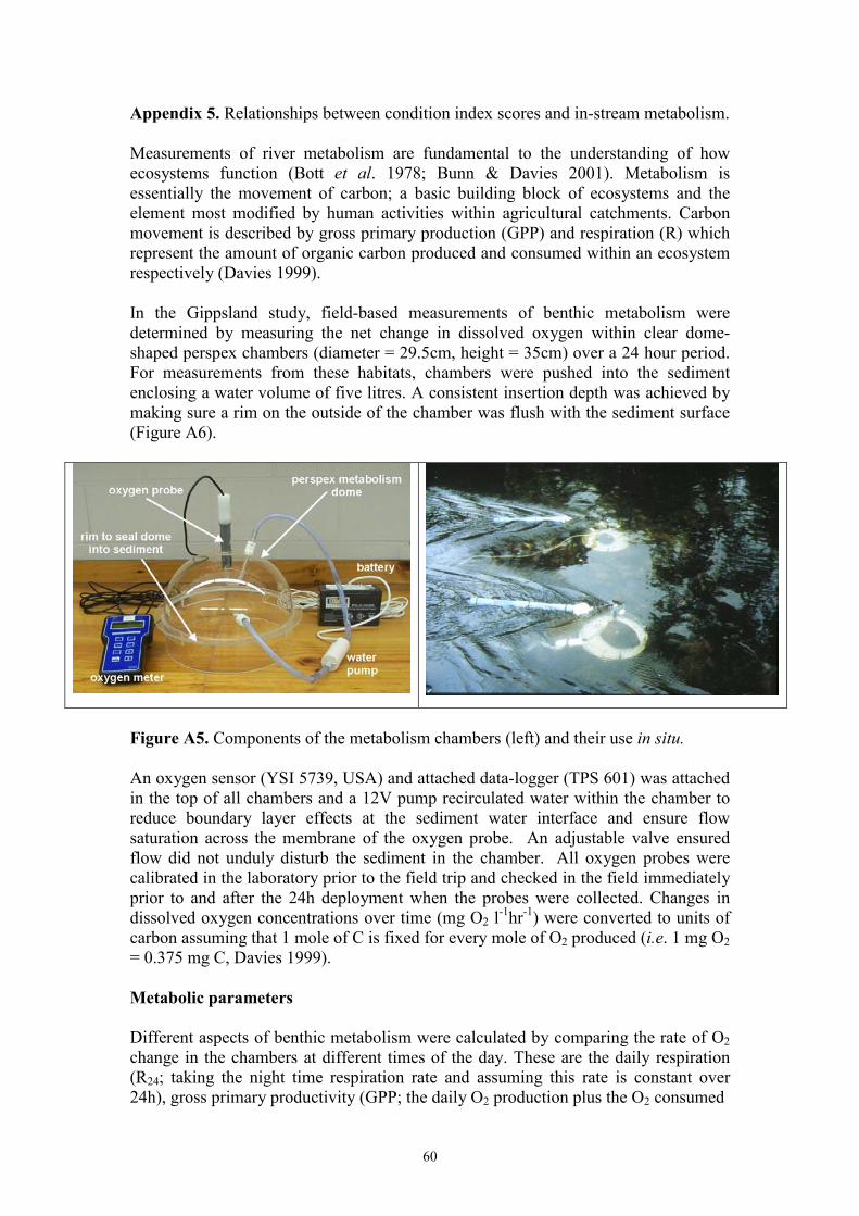
60
Appendix 5. Relationships between condition index scores and in-stream metabolism.
Measurements of river metabolism are fundamental to the understanding of howecosystems function (Bott et al. 1978; Bunn & Davies 2001). Metabolism isessentially the movement of carbon; a basic building block of ecosystems and theelement most modified by human activities within agricultural catchments. Carbonmovement is described by gross primary production (GPP) and respiration (R) whichrepresent the amount of organic carbon produced and consumed within an ecosystemrespectively (Davies 1999).
In the Gippsland study, field-based measurements of benthic metabolism weredetermined by measuring the net change in dissolved oxygen within clear dome-shaped perspex chambers (diameter = 29.5cm, height = 35cm) over a 24 hour period.For measurements from these habitats, chambers were pushed into the sedimentenclosing a water volume of five litres. A consistent insertion depth was achieved bymaking sure a rim on the outside of the chamber was flush with the sediment surface(Figure A6).
Figure A5. Components of the metabolism chambers (left) and their use in situ.
An oxygen sensor (YSI 5739, USA) and attached data-logger (TPS 601) was attachedin the top of all chambers and a 12V pump recirculated water within the chamber toreduce boundary layer effects at the sediment water interface and ensure flowsaturation across the membrane of the oxygen probe. An adjustable valve ensuredflow did not unduly disturb the sediment in the chamber. All oxygen probes werecalibrated in the laboratory prior to the field trip and checked in the field immediatelyprior to and after the 24h deployment when the probes were collected. Changes indissolved oxygen concentrations over time (mg O2 l-1hr-1) were converted to units ofcarbon assuming that 1 mole of C is fixed for every mole of O2 produced (i.e. 1 mg O2= 0.375 mg C, Davies 1999).
Metabolic parameters
Different aspects of benthic metabolism were calculated by comparing the rate of O2change in the chambers at different times of the day. These are the daily respiration(R24; taking the night time respiration rate and assuming this rate is constant over24h), gross primary productivity (GPP; the daily O2 production plus the O2 consumed
61
by respiration during the day, calculated using the night time respiration rate), netdaily metabolism (NDM; equal to GPP - R24) and the P/R ratio (GPP divided by R24).If a system has NDM (i.e. P/R > 1), it is a net producer of organic carbon i.e. accruingbiomass and termed "autotrophic". If P/R = 1 the system is in steady state (NDM = 0)and, if NDM (i.e. P/R < 1) the system is a net consumer of organic carbon or"heterotrophic". The photoperiod was determined as the part of the day when GPPexceeded net respiration.
Results
All the sites studied were net consumers of carbon (e.g. negative NDM) except onesite that had slightly positive rates (85mgC.m-2.day-1). The dominance of heterotrophy(negative NDM) is typical of upland streams across of arrange of Australian biomes(Bunn & Davies 2000). Overall, rates of all metabolic processes measured in thestudy sites were elevated compared to forested systems elsewhere in Australia (Bunnet al. 1999); this undoubtedly reflects the nutrient-enriched status of the streams inGippsland.
Gross Primary Production
Mean rates of GPP (in mgC.m-2day-1) ranged from 12-26 through to 1083-2105. Thisrepresents a considerable gradient of metabolism values and indicates fundamentalchanges in ecosystem processes across the study sites. Rates of GPP were positivelycorrelated to measurements of the natives sub index (r=0.65, p<0.001). In smallstreams, GPP is typically regulated by below canopy light (Bunn et al. 1998; Mosischet al. 2001).
Respiration
Rates of respiration (R24) were elevated at most sites; reflecting the dominance ofheterotrophy. Rates ranged from 487 mgC.m-2day-1 to 3880 mgC.m-2day-1. Again,this is a range of values across an order of magnitude, which represents a gradient ofecosystem conditions.
Net Daily Metabolism
Net daily metabolism (NDM) is the absolute rate of metabolism. NDM values wereall negative indicating sites as net consumers of carbon. Values ranged from positivevalues to substantial negative values (-2309 mgC.m-2day-1). NDM was correlated torespiration; indicating respiration dominated overall NDM.
Temperature range
Daily ranges in temperature were highly variable amongst sites. Lowest dieldifference was 1.3 oC. Highest diel differences in temperature were recorded at twosites 8.3 oC and 5.1 oC respectively. Elevated temperatures can directly impact on thetemperature-tolerance of aquatic species and through reduction of dissolved oxygen(DO) able to held in solution (as % saturation).
62
Conclusions
Overall rates of metabolism were relatively elevated undoubtedly reflecting theambient conditions of elevated nutrient status. The strong relationship between thedominant metabolic process (respiration) indicates the rapid assessment technique isrelated to river health. In contrast to the rapid assessment approach, the measurementof metabolism can be technically-difficult.
ReferencesBott, T. L., Brock, J. J., Cushing, C. E., Gregory, S. V., King, D. & Petersen, R. C.
(1978). A comparison of methods for measuring primary productivity andcommunity respiration in streams. Hydrobiologia. 60: 3-12.
Bunn, S.E., Davies, P.M. & Mosisch, T. (1999). Ecosystem measures of river healthand their response to riparian and catchment degradation. Freshwater Biology.41: 333-345.
Bunn, S.E. & Davies, P.M. (2000). Biological processes in running waters and theirimplications for the assessment of ecological integrity. Hydrobiologia422/423: 61-70.
Bunn, S.E. & Davies, P.M. (2001). Dryland river ecosystems and forest river ecology:implications for management. Inland Rivers Workshop. Alice Springs 27-28March 2001.
Bunn, S.E., Davies, P.M. & Mosisch. T.D. (1998). Contribution of algal carbon tostream food webs. Journal of Phycology 34: 10-11.
Davies, P.M. (1999). Assessing river health by measuring community metabolism.Rivers for the future. 9: 41-43. Land and Water Resources Research andDevelopment Corporation, Canberra, Australia. ISSN 1325-1953.
Mosisch, T., Bunn, S.E. & Davies, P.M. (2001). The relative importance of shading and nutrients on algal production in subtropical streams. Freshwater Biology46: 1269-1278.
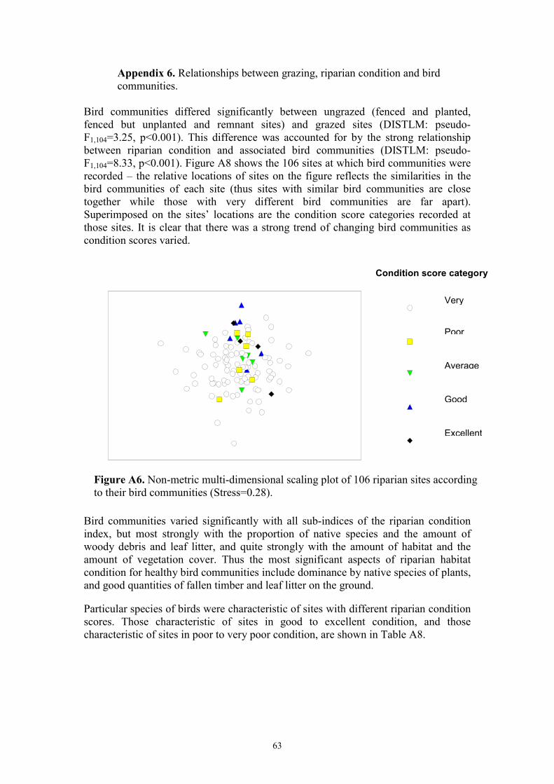
63
Appendix 6. Relationships between grazing, riparian condition and birdcommunities.
Bird communities differed significantly between ungrazed (fenced and planted,fenced but unplanted and remnant sites) and grazed sites (DISTLM: pseudo-F1,104=3.25, p<0.001). This difference was accounted for by the strong relationshipbetween riparian condition and associated bird communities (DISTLM: pseudo-F1,104=8.33, p<0.001). Figure A8 shows the 106 sites at which bird communities wererecorded – the relative locations of sites on the figure reflects the similarities in thebird communities of each site (thus sites with similar bird communities are closetogether while those with very different bird communities are far apart).Superimposed on the sites’ locations are the condition score categories recorded atthose sites. It is clear that there was a strong trend of changing bird communities ascondition scores varied.
Bird communities varied significantly with all sub-indices of the riparian conditionindex, but most strongly with the proportion of native species and the amount ofwoody debris and leaf litter, and quite strongly with the amount of habitat and theamount of vegetation cover. Thus the most significant aspects of riparian habitatcondition for healthy bird communities include dominance by native species of plants,and good quantities of fallen timber and leaf litter on the ground.
Particular species of birds were characteristic of sites with different riparian conditionscores. Those characteristic of sites in good to excellent condition, and thosecharacteristic of sites in poor to very poor condition, are shown in Table A8.
Very
Poor
Average
Good
Excellent
Condition score category
Figure A6. Non-metric multi-dimensional scaling plot of 106 riparian sites accordingto their bird communities (Stress=0.28).
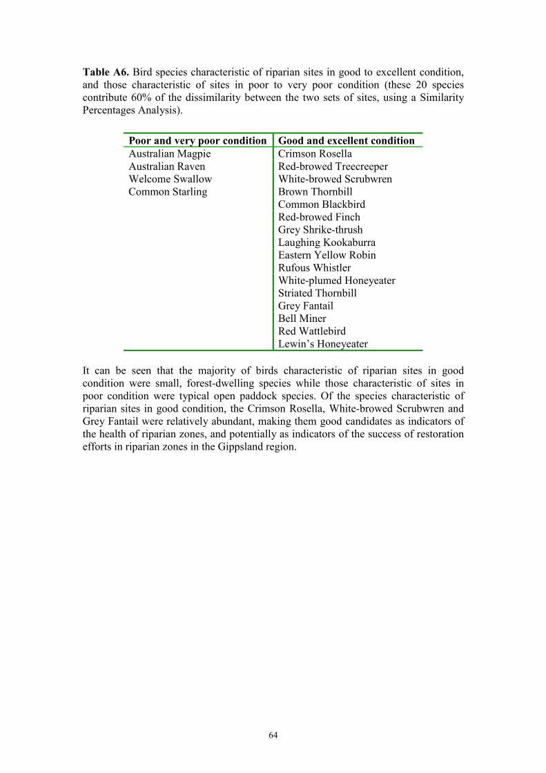
64
Table A6. Bird species characteristic of riparian sites in good to excellent condition,and those characteristic of sites in poor to very poor condition (these 20 speciescontribute 60% of the dissimilarity between the two sets of sites, using a SimilarityPercentages Analysis).
Poor and very poor condition Good and excellent conditionAustralian Magpie Crimson RosellaAustralian Raven Red-browed TreecreeperWelcome Swallow White-browed ScrubwrenCommon Starling Brown Thornbill
Common BlackbirdRed-browed FinchGrey Shrike-thrushLaughing KookaburraEastern Yellow RobinRufous WhistlerWhite-plumed HoneyeaterStriated ThornbillGrey FantailBell MinerRed WattlebirdLewin’s Honeyeater
It can be seen that the majority of birds characteristic of riparian sites in goodcondition were small, forest-dwelling species while those characteristic of sites inpoor condition were typical open paddock species. Of the species characteristic ofriparian sites in good condition, the Crimson Rosella, White-browed Scrubwren andGrey Fantail were relatively abundant, making them good candidates as indicators ofthe health of riparian zones, and potentially as indicators of the success of restorationefforts in riparian zones in the Gippsland region.
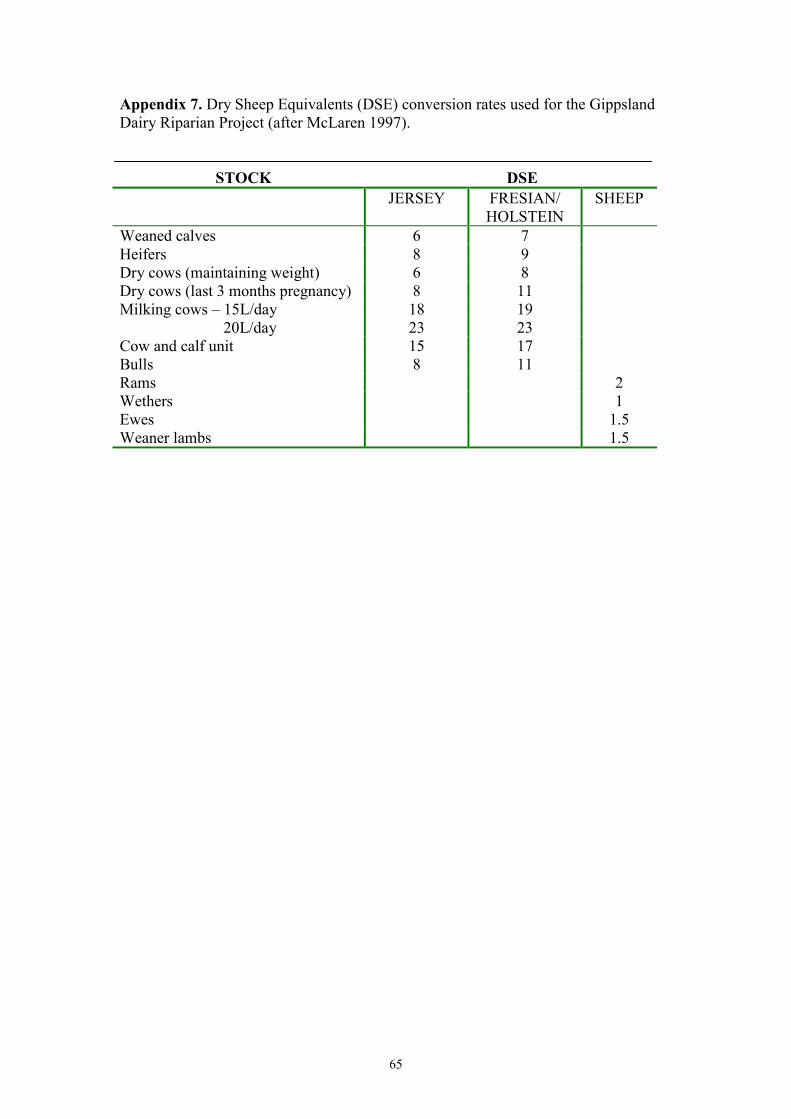
65
Appendix 7. Dry Sheep Equivalents (DSE) conversion rates used for the GippslandDairy Riparian Project (after McLaren 1997).
STOCK DSEJERSEY FRESIAN/
HOLSTEINSHEEP
Weaned calves 6 7Heifers 8 9Dry cows (maintaining weight) 6 8Dry cows (last 3 months pregnancy) 8 11Milking cows – 15L/day 18 19 20L/day 23 23Cow and calf unit 15 17Bulls 8 11Rams 2Wethers 1Ewes 1.5Weaner lambs 1.5

66
Appendix 8. (a) Mean scores for condition sub-indices against overall condition categories. See below for statistical analysis of data.

67
Appendix 8. (b) Stepwise regression of sub-indices on total condition index scores
ModelAdjusted R
squareSE of theestimate Predictors
1 0.896 3.091 NATIVES2 0.934 2.457 NATIVES, HABITAT3 0.970 1.686 NATIVES, HABITAT, DEBRIS4 0.994 0.770 NATIVES, HABITAT, DEBRIS, SPECIES5 1 0 NATIVES, HABITAT, DEBRIS, SPECIES, COVER

68

69
Recommended