GOMOS CALIBRATION ON ENVISAT – STATUS ON DECEMBER 2002
Gilbert Barrot (1), Jean-Loup Bertaux(2), Renaud Fraisse (3), Antoine Mangin(1), Alain Hauchecorne(2) ,
Odile Fanton d’Andon(1) , Francis Dalaudier(2), Charles Cot(2) , Erkki Kyrölä(4), Johanna Tamminen(4),
Bertrand Théodore(1), Didier Fussen(5), Rob Koopman(6), Lidia Saavedra(6), Paul Snoeij(6)
(1) ACRI-ST,260, route du Pin Montard, Sophia-Antipolis Cedex BP 234 F-06904 FRANCE, [email protected] (2) Service d’Aéronomie du CNRS BP3 - 91371 - Verrieres le Buisson Cedex F- FRANCE, [email protected]
(3)Astrium SAS, 31402 TOULOUSE cedex FRANCE, [email protected] (4) FMI, P.O.BOX 503, FIN-00101 Helsinki FINLAND, [email protected]
(5) IASB, Avenue Circulaire 3 B-1180 Brussels Belgium , [email protected] (6) ESA ESTEC and ESRIN centres
ABSTRACT/RESUME
This paper summarises the status of the GOMOS calibration assessed by the GOMOS CAL/VAL team after nine
months of the instrument in-flight life. The first GOMOS occultation was successfully measured on March 22, 2002, starting the calibration and verification activity phase. Since this date, more than 50000 occultations have been
performed until end of 2002. The GOMOS CAL team was in charge of i) the full in-flight calibration and re-
characterisation of GOMOS, ii) all the activities required to achieve the complete verification of the level 1b processing
models, including: algorithms, auxiliary products, instrument performance, measurements geolocation and validation of
the atmosphere related parameters. Lastly, the GOMOS CAL team provided the relevant inputs to the GOMOS mission planning monitoring, and to the future routine calibration operations and validation activities. The GOMOS instrument
in-flight performances are globally very good, in line with expected budget, except for CCD behaviour (hot pixels,
RTS). All measured performances are described hereafter, together with assessment methodology and
recommendations.
1 GOMOS INSTRUMENT PERFORMANCE
1.1 Brief reminder of the GOMOS instrument measurement concept
The GOMOS operating principle relies on the stellar occultation method, which consists to observe a star outside the
atmosphere (thus providing a reference stellar spectrum) and track it as it sets through the atmosphere (thus providing
spectra with absorption features). When these occulted spectra are divided by the reference spectrum, nearly calibration-
free horizontal transmission spectra are obtained, assuming the instrument response function does not change during
one occultation; lasting typically 30 to 40 seconds. These transmissions provide the basis for retrieval of atmospheric
constituents density profiles, which benefits from the fact that observing the star light confines the measurement to a "thin" well-defined volume.
1.2 Method
The verification of the instrument health and performance activities have started on March 22, 2002, just after the
SODAP phase which had validated the correct behaviour of the Service Module, Payload Equipment Bay and Payload
instruments, checked the GOMOS level 0 products format, and roughly verified that the instrument can be commanded
as expected.
Due to launch and in-orbit environments, several instrument characteristics may have been modified like the instrument
response function, thermal distortion and settling of the optical bench, ... and this calls for calibration and monitoring of
GOMOS parameters behaviour and performance: electronic gain chain, read-out noise and offset, non linearity, dark
charge, pixel response non-uniformity, radiometric sensitivity, spectral line spread function, wavelength assignment,
vignetting, and straylight.
All measured performances are described hereafter. The method and tools used during the Calibration phase are briefly
described. Then, the measurement results are analysed and compared to the expectations and the specifications. Finally,
for each calibration parameter, recommendations are given for the routine mission.
__________________________________________________________________________________________________________Proc. of Envisat Validation Workshop, Frascati, Italy, 9 – 13 December 2002 (ESA SP-531, August 2003)

1.3 Acquisition, detection and pointing performance
The objective is to verify if the GOMOS instrument is able to acquire and track stars outside and through the
atmosphere. This task will allow to assess tracking limits (altitude range versus star magnitude) and to verify the dynamic component of the pointing errors that contribute to the dynamic spatial and spectral Line Spread Functions.
The detection and acquisition performance have been analysed:
• during SODAP, for the acquisition and tracking ranges
• by analysing the successful acquisition of faint stars
The mispointing observed during SODAP is linked with the acquisition cone. It has been analysed using the Most
Illuminated Pixel position in detection given in the auxiliary data.
Tracking capability has been analysed using the SATU noise monitoring (auxiliary data) and looking at the altitude
corresponding to the tracking loss.
The tools used for these analyses are mainly the Calibration software CALEX and the GOMOS processing prototype
GOPR.
The acquisition range and tracking Field Of View are consistent with the delivery status. Margins have been taken in
order to be sure not to hit the limits.
Table 1: Ranges and duration performance
10 s< 7 s8.1 sCentring duration
2°/s> 2°/s> 2°/sRallying speed
7°; 5°> 7.1°; 5.3°7.4°; 6.5°Tracking FOV
-10 – 90°
62 – 68°
> -10.8 – 90.8°
> 62 – 68.8°
-11 – 91°
61.7 – 69°
SFM range
specmeasuredexpectedAcquisition
10 s< 7 s8.1 sCentring duration
2°/s> 2°/s> 2°/sRallying speed
7°; 5°> 7.1°; 5.3°7.4°; 6.5°Tracking FOV
-10 – 90°
62 – 68°
> -10.8 – 90.8°
> 62 – 68.8°
-11 – 91°
61.7 – 69°
SFM range
specmeasuredexpectedAcquisition
The duration of rallying and centring phases are also confirmed.
For the performance in detection, a limited number of stars have been tested and the detection threshold has been kept
to a safe value. Indeed, a too small value can lead to a class C anomaly which put instrument in Refuse mode. Even if
there is no danger for the instrument, we decided not to test the limits of detection. Indeed, the actual number of tested
stars is already much larger than the scientific need (and than the specification).
Table 2: Detection probability results
3.2> 44.4Cold star bright limb
1.6> 3.22.2Hot star bright limb
4> 4.56.8Cold star dark limb
2.4> 3.74.6Hot star dark limb
specmeasuredexpectedDetection capability
3.2> 44.4Cold star bright limb
1.6> 3.22.2Hot star bright limb
4> 4.56.8Cold star dark limb
2.4> 3.74.6Hot star dark limb
specmeasuredexpectedDetection capability
Acquisition mispointing performance is the difference between expected and observed position of the star in the SATU FOV after rallying. The expected value is less than 0.16°. The observed value during SODAP is 0.3° in elevation 'El)
and 0.1° in azimuth (Az).
The analysis of the unexpected mispointing in Elevation has shown:
• a contribution due to a forgetting of GOMOS optical frame / GOMOS reference cube alignment in the
configuration matrix (0.1° in elevation and 0.06° in azimuth).
• a possible impact of the gravity compensation of the mechanism. A shift of a few tens of microns could easily induce a bias of 0.1° in elevation.
• a possible contribution due to the calibration curves of SFA angles.

This difference has been corrected and the stars are now detected at the centre of the SATU. No trend has been
observed since then (Fig. 1).
Fig. 1: Position of the detection of stars in SATU before and after the correction.
Tracking noise and robustness: the expected value of the SATU noise equivalent angle in dark limb (at 100 Hz) is 13
µrad (3s) for a specification of 18 µrad. The measured value is better than 3 µrad in dark limb (DL) and 10 µrad in
bright limb (BL) (35 km altitude). Noise is less than 1 µrad (3σ) for Sirius.
Fig. 2 presents the mispointing error reported by the SATU data. Movement in elevation around 100 km is due to the presence of the O2 emission layer. The refraction effect can be seen in elevation below 40 km.
-50
-40
-30
-20
-10
0
10
20
30
40
50
0 20 40 60 80 100 120 140
Elevation
Azimuth
µrad SATU noise at 100 Hz for Sirius
Dark limb
km
-50
-40
-30
-20
-10
0
10
20
30
40
50
0 20 40 60 80 100 120 140
Elevation
Azimuth
µrad SATU noise at 100 Hz for ID 154,
Bright limb
km
Fig. 2: SATU noise equivalent angle for two different stars in dark and bright limb
The altitude range has been analysed for many of the stars already acquired.
The average minimum altitude is 15 km in dark limb and 22 km in bright limb, better than expected. It is nearly not dependent on magnitude since the tracking loss is mainly due to the refraction and the scintillation that depend on the
atmosphere conditions.
The minimum altitude reached in tracking is below 5 km for the brightest stars.
The refraction induces a displacement on the SATU up to 20 µrad at 10 km.
The effect on the spectrum (bending in UV) appears when flux is already nearly completely absorbed by atmosphere.

The values of the ranges (in acquisition/tracking) and the durations (in rallying/ centring) that have been confirmed have
been implemented in the RGT Operational Parameter file. Margins have been taken with respect to the GOMOS
expected capability but should be kept for the lifetime since it is already larger than the scientific need. These performances are not expected to change during the life. Only an analysis of the possible anomalies is required.
For detection, the number of stars which can be acquired is larger than 500 (already enough for the mission). The
detection threshold (15 LSB) should be kept like this and should anyway not be decreased below 5 LSB since there
could be a risk of a class C anomaly.
1.4 Optomechanical and thermal performance
The tool used for these analyses is mainly the CALEX calibration software.
Different instrument modes are used for these parameters:
• Analysis through spatial spread monitoring mode for the spatial displacement. The barycentre computation
leads to potential adjustment of integration area size and position (band setting task). Spatial extension of the
star is an indication for monitoring the defocus.
• Analysis through occultation mode for the spectral displacement (wavelength assignment). The wavelength
assignment variation is computed by correlation of spectra.
• Analysis through occultation mode for the SATU/Slit displacement. We measure the comparison of total flux
on each CCD when the star is artificially moved on the SATU.
The optomechanical displacements due to the launch are less than 0.3 pixels for all CCD.
The thermal influence on each of these performances has been measured during different cooling phases (from +10°C
down to around –4°C). At +10°, the thermal behaviour of GOMOS is as expected, close to the "Beginning Of Life hot" thermal case. No anomaly or curious behaviour has been observed. The variations along orbit are very consistent with
the model.
Fig. 3 presents the variation of the temperature for several GOMOS elements after the last cooling phase. The variation
for DMSA and DMSB (where the CCDs are) is close to 0.35°. Knowing the thermal sensitivity of the spectrometer
pixels, this variation leads to an inaccuracy of 5 to 6 % on the dark charge level. As the accuracy of the thermistor
measurements (coding accuracy) is also 0.40°C, the final inaccuracy may be of the order of 10 %.
-12
-10
-8
-6
-4
-2
0
16:26:24 16:40:48 16:55:12 17:09:36 17:24:00 17:38:24 17:52:48 18:07:12
Temperature variation of OB units
over one orbit°C
time
OSB
OSA
SATU1OB structure
DMSA
OBD
DMSB
SATU2
DMFP
Bright limb
Fig. 3: Temperature variation of OB units over one orbit
The displacements with temperature variation are inside the expected budget (0.5 pixel/10°C for DMSA and 0.1 pixel
for DMSB). The variation during one orbit is lower than 0.03 pixel. The spectral stability is better than expected.
The optical performance are as expected. The size of the star is included in 4 lines (at 95%).
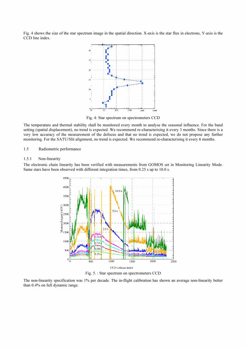
Fig. 4 shows the size of the star spectrum image in the spatial direction. X-axis is the star flux in electrons, Y-axis is the
CCD line index.
Fig. 4: Star spectrum on spectrometers CCD
The temperature and thermal stability shall be monitored every month to analyse the seasonal influence. For the band setting (spatial displacement), no trend is expected. We recommend re-characterising it every 3 months. Since there is a
very low accuracy of the measurement of the defocus and that no trend is expected, we do not propose any further
monitoring. For the SATU/Slit alignment, no trend is expected. We recommend re-characterising it every 6 months.
1.5 Radiometric performance
1.5.1 Non-linearity
The electronic chain linearity has been verified with measurements from GOMOS set in Monitoring Linearity Mode.
Same stars have been observed with different integration times, from 0.25 s up to 10.0 s.
Fig. 5. : Star spectrum on spectrometers CCD
The non-linearity specification was 1% per decade. The in-flight calibration has shown an average non-linearity better
than 0.4% on full dynamic range.

The electronic chain offset is also calibrated using the same measurements. The stability of the offset computed from
calibrations performed at several times is better than 0.1 ADU.
1.5.2 Non-uniformity of pixel response
The pixel response non-uniformity has been measured at pixel and at band level using the Uniformity monitoring mode
and the occultation fictive star mode of the GOMOS instrument. The measurements have been made in bright limb
conditions.
The tools used for these analyses are mainly the calibration software CALEX.
The radiometric uniformity performance is consistent with expected. There is no degradation of the pixel response even
for the pixels showing a degraded dark current.
One bad pixel in DMSA2 (-26%) already seen on ground has not moved nor degraded.
The interferences on IR spectrometers present the same shape and amplitude as on ground. Fig. 6 presents the PRNU
observed on DMSB2 (IR2).
Fig. 6: Interference pattern observed on IR2 spectrometer
The slit profile measurement is consistent with ground.
Table 3: Non-uniformity results
Radiometric Uniformity UV VIS IR1 IR2
mean ground 1.7% 1.7% 1.9% 12%
flight 1.4% 1.6% 2.4% 12%
max ground 3% 3.6% 6.8% 42%
flight < 4% 4.3% 6.6% 40%
No trend has been measured yet for this parameter.
The response non-uniformity shall be monitored every month, especially in IR, where interferences position is
influenced by temperature. No variation is expected if temperature is stable.
1.5.3 Radiometric calibration and stability
The radiometric calibration is performed by comparing the stellar spectra with external reference sources. Good
consistency between measurements and on-ground characterisation is observed.

Fig. 7: Radiometric calibration
Variation level between orbits is compatible with the theoretical noise.
Very stable radiometry in all the spectral coverage of GOMOS: as a consequence, the complete spectral range of
GOMOS is now considered as valid and used in the ground processing. No trend observed yet.
It should be noted that the absolute radiometric calibration has no significant impact on the level 2 products (species density profiles).
1.6 Wavelength assignment
The spectral calibration is performed by comparing the spectral assignment of several columns with external well-
known reference sources (see Fig. 8). It should be noted that a vacuum wavelength scale is adopted for GOMOS. While
one column per CCD becomes the reference column, the other calibrated columns are used to update the spectral
dispersion law of the spectrometer. Lastly, the spectral assignment of any CCD column is done by using the reference column and the spectral dispersion law.
Fig. 8: Wavelength calibration
The wavelength assignment found by this method is consistent with the spectral assignment of the cross-sections used
in the level 2 processing (see Fig. 9: comparison of the measured and modelled transmission at 26.6 km in SPA1
spectral range). The accuracy of the wavelength calibration is of the order of 1/30 pixel.

Fig. 9. : Transmission model (green) versus measured transmission (blue)
No trend has been observed during several weeks. However, due to the high sensitivity of the retrieval performance to
the correctness of the wavelength assignment, this calibration shall be carefully and regularly monitored on a monthly
basis.
1.7 CCD dark charge level, hot pixels, RTS
Three operations are performed for the analysis of the GOMOS CCD performance:
• Confrontation of what was expected and calibrated on-ground and what is measured in flight.
• Survey of the temporal evolution of dark charge (DC) value at pixel level and at global level using dark sky
observations
• Spectral analysis (Fourier transform) of dark sky observations.
• Comparison with literature [2].
Fig. 10 shows the two dark signal non-uniformity (DSNU) spectra, normalised with respect to their mean clean dark
charge value. The clean dark charge is the average DC signal over a spectrometer, characterised by its temperature,
assumed to be uniform. All the pixels exhibiting an abnormal behaviour (>3σσσσ) are excluded from the computation of the average and classified as hot pixels. One sees the increase of the number of pixels with high dark charge level as it is
also noted that there were already several pixels presenting this behaviour of high signal on ground.
0.5
1.5
2.5
3.5
4.5
5.5
6.5
7.5
8.5
0 100 200 300 400 500 600 700 800 900 1000 1100 1200 1300 1400 1500 1600 1700 1800 1900 2000 2100 2200 2300
0
1
2
3
4
5
6
7
8normalised DSNU on upper band
ground
flight orbit 792
same scale but with a shift
Fig. 10: DSNU before launch and two months after launch
Before (blue): left vertical axis – After (red): right vertical axis

In September 2002, 60% of the pixels have a mean dark charge higher than 100 electrons, which results in the following
values displayed in the table below for all spectrometers.
Table 4: Mean dark charge per CCD
Mean DC (e) SPA1 SPA2 SPB1 SPB2
Clean dark charge 79 80 93 92
All pixels 215 218 254 223
Using all available Dark Sky Areas observations, we derive the evolution of the mean leakage current on each spectrometer: an increase of 2.4 e/s/day at the current temperature (around -3°) is observed.
In addition to the evolution of the mean dark charge, Random Telegraphic Signal (RTS), defined as an abrupt change in
the average dark charge level for a given pixel, has been observed. The observations indicate a high variability of RTS
duration and stability. They have been compared to literature [2] and made appear similarities (although RTS level are
higher in the present case) with published observations.
Fig. 11 presents the temporal evolution of the dark charge level of several binned pixels during a DSA observation
(dark sky area). RTS events are easily visible on these curves.
Fig. 11: RTS occurrences
Fig. 12 presents several spectra of star #018 measured outside the atmosphere (each spectrum is in fact the averaged
spectrum over 10 measured spectra at the beginning of one occultation) between absolute orbits 2900 and 2920, in part
of the spectral range of the spectrometer SPA2 (570-650 nm).
Fig. 12. : Reference star spectra (star #018, SPA2) and RTS occurrences
The analysis performed during the CAL/VAL phase has shown that 500 to 600 pixels per band (i.e. 25 percents of the
samples) are affected by RTS events during one orbit (i.e. between two DC map calibrations at orbit level). The mean
variation of the DC level is close to 65 electrons (1 sigma).
Fig. 13 presents an example of the temporal variation of the dark charge level due to RTS. Two dark charge maps
measured at one week interval (mean dark charge around 250 e-) are compared.
Fig. 13. : temporal variation of the DC level due to RTS
A preliminary study of the impact on the level 2 products has been performed and shows a degradation of several
percents on ozone and other species. The cooling of the CCD to decrease this effect by decreasing the mean dark charge
level has been performed. Anyway, the minimum temperature reached lead to a state where the RTS has still an
important impact on the quality of the retrieval of several species (especially NO2, NO3).
A dark charge calibration at orbit level (one DC map measured every orbit) has also been programmed and implemented in the level 1b processing chain. Using this dark charge map brings a clear improvement, of the order of a
recovery of half the degradation due to RTS (conclusion reached from the analysis of a set of end to end simulations,
using the GOMOS simulator, performed during the CAL/VAL activities).
1.8 Signal modulation
When analysing dark sky observations, an oscillating regular parasitic signal has been detected in addition to the dark charge:
• A modulation signal of +/-1.4 ADU has been found for spectrometer A1.
• A similar modulation signal of +/-0.76 ADU has been found for spectrometer A2.
• No modulation has been detected for spectrometers B1 and B2.
An algorithm has been prototyped to remove the modulation. It is routinely exploited for calibration analysis.
Considering the improvement in the variance obtained with this algorithm, its implementation in the nominal GOMOS processing chain has been done.
The total static variance (i.e. excluding photon noise and including electronic chain noise and quantisation noise) is
significantly different from the on ground values for the UVIS spectrometers when the correction for signal modulation
is applied. The resulting variance for each spectrometer is given in the table below.
Table 5: Total measured static variance (i.e. excluding photon noise) in e2
SPA1 SPA2 SPB1 SPB2
602 525 297 339
Post-launch characterisation of static noise contributors
after correction for modulation signal
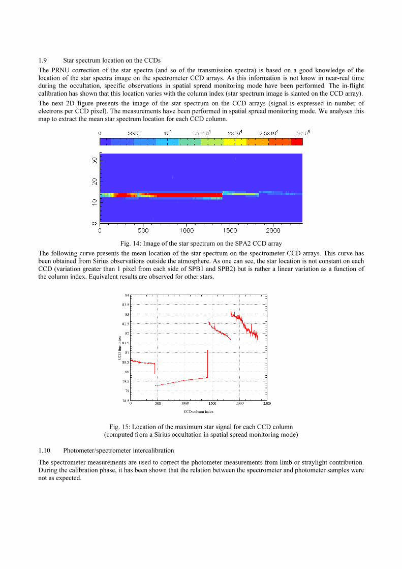
1.9 Star spectrum location on the CCDs
The PRNU correction of the star spectra (and so of the transmission spectra) is based on a good knowledge of the
location of the star spectra image on the spectrometer CCD arrays. As this information is not know in near-real time during the occultation, specific observations in spatial spread monitoring mode have been performed. The in-flight
calibration has shown that this location varies with the column index (star spectrum image is slanted on the CCD array).
The next 2D figure presents the image of the star spectrum on the CCD arrays (signal is expressed in number of
electrons per CCD pixel). The measurements have been performed in spatial spread monitoring mode. We analyses this
map to extract the mean star spectrum location for each CCD column.
Fig. 14: Image of the star spectrum on the SPA2 CCD array
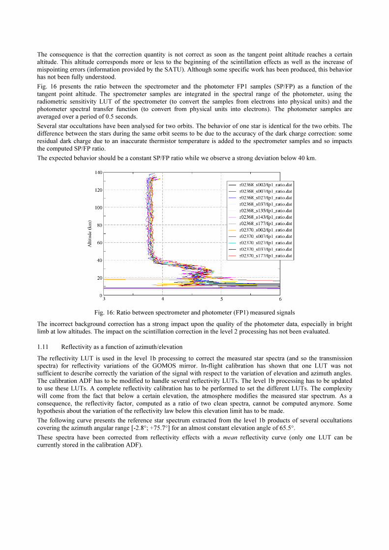
The following curve presents the mean location of the star spectrum on the spectrometer CCD arrays. This curve has
been obtained from Sirius observations outside the atmosphere. As one can see, the star location is not constant on each
CCD (variation greater than 1 pixel from each side of SPB1 and SPB2) but is rather a linear variation as a function of
the column index. Equivalent results are observed for other stars.
Fig. 15: Location of the maximum star signal for each CCD column (computed from a Sirius occultation in spatial spread monitoring mode)
1.10 Photometer/spectrometer intercalibration
The spectrometer measurements are used to correct the photometer measurements from limb or straylight contribution.
During the calibration phase, it has been shown that the relation between the spectrometer and photometer samples were
not as expected.
The consequence is that the correction quantity is not correct as soon as the tangent point altitude reaches a certain
altitude. This altitude corresponds more or less to the beginning of the scintillation effects as well as the increase of
mispointing errors (information provided by the SATU). Although some specific work has been produced, this behavior has not been fully understood.
Fig. 16 presents the ratio between the spectrometer and the photometer FP1 samples (SP/FP) as a function of the
tangent point altitude. The spectrometer samples are integrated in the spectral range of the photometer, using the
radiometric sensitivity LUT of the spectrometer (to convert the samples from electrons into physical units) and the
photometer spectral transfer function (to convert from physical units into electrons). The photometer samples are
averaged over a period of 0.5 seconds.
Several star occultations have been analysed for two orbits. The behavior of one star is identical for the two orbits. The
difference between the stars during the same orbit seems to be due to the accuracy of the dark charge correction: some
residual dark charge due to an inaccurate thermistor temperature is added to the spectrometer samples and so impacts
the computed SP/FP ratio.
The expected behavior should be a constant SP/FP ratio while we observe a strong deviation below 40 km.
Fig. 16: Ratio between spectrometer and photometer (FP1) measured signals
The incorrect background correction has a strong impact upon the quality of the photometer data, especially in bright
limb at low altitudes. The impact on the scintillation correction in the level 2 processing has not been evaluated.
1.11 Reflectivity as a function of azimuth/elevation
The reflectivity LUT is used in the level 1b processing to correct the measured star spectra (and so the transmission spectra) for reflectivity variations of the GOMOS mirror. In-flight calibration has shown that one LUT was not
sufficient to describe correctly the variation of the signal with respect to the variation of elevation and azimuth angles.
The calibration ADF has to be modified to handle several reflectivity LUTs. The level 1b processing has to be updated
to use these LUTs. A complete reflectivity calibration has to be performed to set the different LUTs. The complexity
will come from the fact that below a certain elevation, the atmosphere modifies the measured star spectrum. As a
consequence, the reflectivity factor, computed as a ratio of two clean spectra, cannot be computed anymore. Some hypothesis about the variation of the reflectivity law below this elevation limit has to be made.
The following curve presents the reference star spectrum extracted from the level 1b products of several occultations
covering the azimuth angular range [-2.8°; +75.7°] for an almost constant elevation angle of 65.5°.
These spectra have been corrected from reflectivity effects with a mean reflectivity curve (only one LUT can be
currently stored in the calibration ADF).

As one can see on Fig. 17, the correction is not perfect. One can also notice that the relative differences are not identical
along the spectrum (obviously there is less difference around column 500 than around column 400 or 450).
Fig. 17: Reference star spectrum of Sirius between orbits 2250 and 2993
Fig. 18 presents two reflectivity curves for spectrometer A. The X-axis is the wavelength assignment of the CCD
column expressed in nm. The Y-axis is the reflectivity curve expressed in %. The pink curve corresponds to an azimuth
of 54.5° while the dark blue one corresponds to an azimuth angle of 75.7°. The difference between these two curves can be of the order of 0.5%.
-2.000
-1.500
-1.000
-0.500
0.000
0.500
1.000
1.500
2.000
200.000 300.000 400.000 500.000 600.000 700.000
Fig. 18: Computed reflectivity factors for two SFM azimuth angles
The same effect is visible when the elevation varies for a constant azimuth angle. This is the case during any
occultation. The current status leads to an error of 1% in several spectral intervals of the transmission spectra.
1.12 Background and straylight
The analysis and conclusions concerning these two items can be found in [1].
2 VALIDATED AND TUNED LEVEL 1B PROCESSING CHAIN
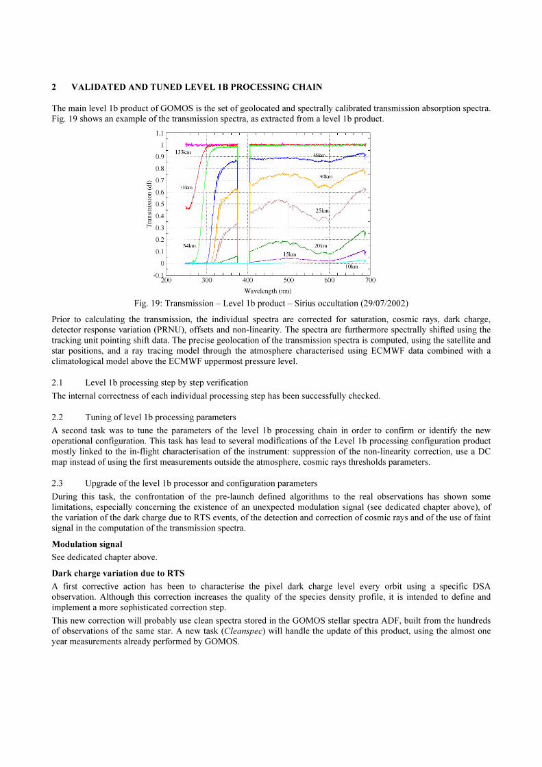
The main level 1b product of GOMOS is the set of geolocated and spectrally calibrated transmission absorption spectra.
Fig. 19 shows an example of the transmission spectra, as extracted from a level 1b product.
Fig. 19: Transmission – Level 1b product – Sirius occultation (29/07/2002)
Prior to calculating the transmission, the individual spectra are corrected for saturation, cosmic rays, dark charge, detector response variation (PRNU), offsets and non-linearity. The spectra are furthermore spectrally shifted using the
tracking unit pointing shift data. The precise geolocation of the transmission spectra is computed, using the satellite and
star positions, and a ray tracing model through the atmosphere characterised using ECMWF data combined with a
climatological model above the ECMWF uppermost pressure level.
2.1 Level 1b processing step by step verification
The internal correctness of each individual processing step has been successfully checked.
2.2 Tuning of level 1b processing parameters
A second task was to tune the parameters of the level 1b processing chain in order to confirm or identify the new
operational configuration. This task has lead to several modifications of the Level 1b processing configuration product
mostly linked to the in-flight characterisation of the instrument: suppression of the non-linearity correction, use a DC
map instead of using the first measurements outside the atmosphere, cosmic rays thresholds parameters.
2.3 Upgrade of the level 1b processor and configuration parameters
During this task, the confrontation of the pre-launch defined algorithms to the real observations has shown some
limitations, especially concerning the existence of an unexpected modulation signal (see dedicated chapter above), of
the variation of the dark charge due to RTS events, of the detection and correction of cosmic rays and of the use of faint
signal in the computation of the transmission spectra.
Modulation signal
See dedicated chapter above.
Dark charge variation due to RTS
A first corrective action has been to characterise the pixel dark charge level every orbit using a specific DSA
observation. Although this correction increases the quality of the species density profile, it is intended to define and
implement a more sophisticated correction step.
This new correction will probably use clean spectra stored in the GOMOS stellar spectra ADF, built from the hundreds of observations of the same star. A new task (Cleanspec) will handle the update of this product, using the almost one
year measurements already performed by GOMOS.

Cosmic rays
Based on the analysis of the spectral and temporal variations of the signal, the algorithm led to wrong detections due
mainly to the high temporal signal variations due to large scintillation acting on strong signal flux (most of the problem appeared during the processing of Sirius measurements).
In order not to incorrectly flag full transmission spectra, it has been decided on the short term to increase the cosmic ray
detection threshold in the processing of the Sirius occultations. The consequence is that weak cosmic rays are no more
detected now.
Fig. 20 presents the difference between consecutive measurements during the occultation of Sirius in orbit 2931 (map of
signal gradient). The X-axis represents the CCD column index (the four CCDs are presented on the same graph). The Y-axis represents the measurement number. The unit is ADU. The orbit has been chosen to show real cosmic ray
impacts: Envisat was inside the South Atlantic Anomaly during the observation.
In this representation, a cosmic ray is identified by a couple of red-blue points: an increase of signal due to the cosmic
ray event leads to a positive gradient value (blue pixel) immediately followed by a negative gradient value (red pixel).
The long blue-red lines around measurements 140 are due to a strong variation of the signal itself and obviously not to a
cosmic ray event. If the threshold for cosmic ray detection was set to 50 ADU, all these pixels are wrongly flagged as being contaminated by a cosmic ray event.
Fig. 20: Absolute difference of consecutive GOMOS measurements (orbit 2931)
With the current algorithm (only one single threshold is available), we have to choose between detecting only the strong
cosmic rays and flagging large parts of spectra in case of strong scintillation.
Fig. 21: Absolute difference of consecutive GOMOS measurements (orbit 2934)
A modified algorithm is be proposed to take into account the averaged variations of the measurements in order to
normalise them before cosmic ray detection.

Star spectra location on the CCD
As the calibration ADF contains only one line index (integer number) to define this location, it is not possible to have a
very accurate PRNU correction (see dedicated chapter above).
We propose to replace the line index stored in the current calibration ADF by a LUT giving the line index as a function
of the CCD column index.
As the SPB2 PRNU shows high PRNU between pixels (see the PRNU dedicated chapter above), the choice of using a
constant instead of a LUT may lead to several percents of error on the star spectra after PRNU correction (i.e. also on
the transmission spectra) because we will use an incorrect correction factor. This is especially true in the lower part of
the atmosphere where the instrument mispointings are bigger.
SFM reflectivity factors.
As it has been shown in a previous chapter, the reflectivity factor is a function of the SFM elevation and azimuth
pointing angles.
We propose to implement a reflectivity correction based upon a LUT with azimuth and elevation angles also as input
parameters and not only wavelength as it is done on the current algorithm.
Reference stellar spectra
During the validation phase, it appears that the quality of the density profiles was not satisfactory in the processing of
cold stars. An analysis of the star spectra and associated transmissions shows that negative star spectra combined
together gave positive transmission (especially in the UV part for cold stars) taken into account in the retrieval
processing.
In order to have a short-term corrective action, we have decided to apply a truncation to the reference star spectrum.
The truncation has not been optimised and must be tuned and studied to estimate its impact on the retrieval quality. This threshold has to be optimised. A non-optimised threshold may lead to a lost of accuracy at high altitude for some cold
stars (ozone detection is mostly based on the UV absorption at high altitude).
The current algorithm has also to be modified in order to work for example with a dynamic threshold computed from
the star characteristics.
Fig 22 shows the reference star spectrum for star 52 during orbit 3060. All columns with a flux below 200 electrons (nominal threshold set in the level 1b processing configuration product) will be flagged and the corresponding
transmission values are not used during the spectral inversion step in level 2 processing chain.
Fig. 22: Reference star spectrum (star #052 - abs. orbit 3060)

Fig. 23 shows the comparison of the transmission spectra with and without filtering of the reference star spectrum. The
line is the unfiltered transmission spectrum; the blue symbols represent the filtered transmission.
Fig. 23: Transmission with and without truncation applied
Fig. 24 presents the relative difference between the O3 local density profiles with and without the filtering of the
reference star spectrum.
Fig. 24: Relative difference between the retrieved O3 local density profiles with and without truncation applied
2.4 Level 1b products validation
A specific activity dedicated to the validation of the two level 1b products has started as soon as the level 1b chain was
verified at module level and is still on-going at the time of the calibration review. This activity includes the verification of the data coherency, the validation of geolocation and atmosphere level 1b products, and the validation of stellar
derived products. In particular, the self-coherency of GOMOS products is analysed (e.g. the instrument pointing
direction and the deviation, the transmission at the same location observed by different stars, the photometer data and
the spectrally integrated spectrometer data...).

3 CONCLUSIONS
Regarding the instrument operation, at the time of the validation review, the instrument operability is ready for routine
phase. The altitude range may reach level down to below 5 km. The stellar magnitude range is up to 4.5.
Regarding the instrument performance, instrument in flight is within expected budget, and often better, except for CCD
behaviour. The effects of each contributor to CCD behaviour have been quantified, along with their rate of evolution.
Their impact on the chain performance have made necessary some changes:
1. Three successive cooling of the CCD (orbit 800 / 1050 / 2780) down to -4°
2. New calibration procedure (introduction of regular Dark Sky Area observations)
3. Ad hoc algorithm(s) derivation for correction of the dark charge
Several algorithms of the level 1b processing chain have been specified and are currently implemented in the
operational PDS system. Other actions are still under investigation:
1. Upgrade the background correction in dark (straylight) and bright conditions
2. Improve the estimation of the reference star spectrum
3. Characterise and correct for the reflectivity of the optics
4. Solve the inconsistency found in the intercalibration of spectrometers and photometers 5. Solve the non-uniformity issues for spectrometer B (re-characterisation)
6. Characterise and correct for the RTS
4 REFERENCES
1. Mangin A., et al. Limb and straylight contribution to GOMOS signal – status at end of December 2002, ENVISAT validation workshop proceedings, 2002
2. Proton effects in Charge-Coupled Devices, G.R. Hopkinson, C.J. Dale, and P. W. Marshall, IEEE Transactions in nuclear science, Vol. 43, N°2, April 1996
Recommended