T"echnical Note ~ 6~5c *-
ioiAS ' Cq'"sF TT" $T I T EI"
MA APa

NIASSAcHIUSETTS [NSTITI' TE OF," TE'.INOlYI,O;Y
LINC'OLN I.. A ()IR? AT) R
GRADIENT MATRICES AND MATRIX CALCULATIONS
M. A THANS
Con sul •t
F. C. SCHWEPPE
Group 22
TECHNICAL NOTE 1965-53
17 NOVEMBER 1965
LEXINGTON MASSACHlUSETTS

ABSTRACT
The purpose of this report is to define a useful shorthand notation for dealing
with matrix functions and to use these results in order to compute the gradient
matrices of several scalar functions of matrices.
Accepted for the Air ForceStanley J. WisniewskiLt Colonel, USAFChief, Lincoln Laboratory Office
iii

TABLE 01; CONTENTS
1. INTROI)UCTION I
2. NOTATION 1
3. SPACES 4
4. SOME USEFUL DECOMPOSITIONS OF A MATRIX 5
5. FORMULAE INVOLVING THE UNIT MATRICES E. 7-- 1i
U'. INNER PRODUCTS AND THE TRACE FUNCTION 9
7. D)IFFERENTIALS AND GRADIENT MATRICES 43
8. GRADIENT MATRICES OF TRACE FUNCTIONS 17
9. GRADIENT MATRICES OF DETERMINANT FUNCTIONS 24
W0. PARTITIONED MATRICES 30
TABLE OF GRADIENTS 32
REFERENCES 34

1. INTRODUXCTION
The pur'pose of this report is to present a shorthand notation for matrix mani-
pul•ilion and formulae of differentiation for matrix quantities. The shorthand and
frul;ci aru especially useful whenever one dcdals with the analysis and control of
dynamical systems which are described by matrix differential equations. There are
olhuir aweas of application iat th. cnt-c-l olf matrix di.,°fcrential equations provided
the motivation for this study. References [ 1 ] through [6 ] deal with the analysis and
control of dynamical systems which are described by matrix differential equations.
Much of the material presented in this report is available elsewhere in different
forms; it is summarized herein for the sake of convenience. Two references were
used extensively for the mathematical background; these are Bodewig (Reference [ 7])
and Bellman, (Reference [ 8]).
The organizatian of the report is as follows: In Secticn 2 we present the defi-
nitions of the unit vectors e. and of the unit matrices E ... In Section 3 we indicate-I -ij
the use of the matrices E as basis in the space of n x n mat-'ices. In Section 4 we
present several relations which can be used to decompose a given matrix into its
column and row vectors. Section 5 deals with operations involving the unit vectors
e. and the unit matrices Ei... In Section 6 we show how the trace function can be used•! -ii1
to represent the scalar product of two matrices. In Section 7 we define the differen-
tials of a vector and of a matrix and we also define the motion of a gradient matrix.
Section 8 contains a variety of formulae for the gradient matrix of trace functions.
Section 9 contains relations for the gradient matrix of determinant functions.
Section 10 contains relations involving partitioned matrices. A table summarizing
the gradient formulae of Sections 8 and 9 is also provided.
2. NOTATION
Throughout this report column vectors will be denoted by underlined letters and
matrices by underlined capital letters. The prime (1) will denote transposition.
I

A column vector v with components v,, v2 .... Vn is
v I
V 2
(2i(2,
Vn
In particular, the unit vectors e4 , e2 ,.... e are defined as follows:--1
4 0 0
_e = e = *e . (2.2)El 0 -22 -n
oj 0 4
AnnX m matrix Awith elements a.. (i=1, 2,..., n ; j =1,2 ...2,m) is denoted by-- 1J
a1 a 12 .. . a1M
A a (2.3)
ani an 2 anm
If m=n, then A is square. If A = A' then A is symmetric.
The unit matrices E are square matrices such that all their elements are zero,
except the one located at the i-th row and j-th column which is unity. For example,
2

O I 0 . . . 0
o 0 0 . . (1 1 2 (2.4)
o 0 0 . . . 0
The unit matrix F. is related to the unit vectors c. and c. as follows:-ij -I -. 1
E =0. C1 . (2.5)ij -I -j
The identity matrix I
1 0
I= • •(2.6)
0 0 ... 11
can thus be written
n n
I E, C. (2.7)
The one vector e is defined by
[=
3

The one niatrix E is defined by
E-"" ee (2.9)
The trace of an n x n matrix A is defined by
n
tr [Al = a (2. 10)
i=j
The tracc has the very useful properties
tr[A+B_] = triAI +tr[BI (2. B1)
tr[ABI = tr[BA_ . (2. 42)
The determinant of an n x n matrix A will be denoted by
det [A I
'. SPACES
Wu shall denote by
R n the set of all real column vectors v with n components v V, v2 ... f v
M " the set of all real n X n matricesTin
Both R and M are linear vector spaces.nl liii
The unit vectors e e2 , .. . e n (see Eq. (2. 2)) belong to R and, furthermore,
4

M'f I ha I s Zf I( I i Thuis , c2vury v c R C1if ca c rcp~rsriftcd 1)v
till. I
Siiiitily that tnI trIiispose'. A [ f' ARlO~ k10I NI Wlitll ASC ~I 4I~*~hON hs
-ii 11 - f1i
ii ~ ~ ~ A a Elmti I cnlUU1I~ J~dl a acIli. iiclso
im [ 'Fh Old CU1nsion o VCLIWS i n h iiunino s
NotAui thaT ithXe tratripo c A' offA dcnw b 'OM writte, ay
Af 1.1 *(4
\' ~ 1:

and, so,
' on* (4.2)
We emiphasize that both tpes of vectors a. and a* are column vectors,
We shall now indiczite how one cmi write the elements a.. and the row and coluimnIi
vectors of a matrix A in termis of A and in terms of the unit vectors, e. (see Eq. (2. 2))
, (4.3)
a .~A' e (the transpose of the i-th row of A )(4.4)
a!*e A (the i-tb row vector of A )(4. 5)
C~ A e (the j-th column vector of A 11(4.6)
The eleentci a..ca adlo beO k genra~rted aS foll~OW.:I i
~ a (4.7)
01'1
.e. (4.8)
NLcXt wI shaH IndiCAt the relation of the row and colump. vectors of A to t4e
u!'rnients of A. From Eq(s. (4. 3), (4. 4), (4.51, and (4. 6) w deduce that
"*ij --. O

I1
= (4.9)jl
fl
S- au (4.10)
j=l
aI . = i, -1 . (4.11)
j:. I
Tho inat'Di A can be gencrated ;,s follows: fronm Eqs. (2. 5) and (3. 2) we have
n n n u
a.. C 0/ a., e (4.12)
i=i j=j i=1 j=1
From Eqs. (4. 12), (4. 9), (4. 10) and (4. 11) we obtain
n
A = C (4,1:3)
1;1n
A =ý ia, e' . (4.14)- -j -J
j=1
S. FORMULAE INVOLVING THE UNIT MATRICt,, E..--IJ
First of all if we dufine the Kronucker delta 6.,ij
ij (5. 1)
.o0 if /
S.. .. • -- JM 7

then we have the relation
ee. e=e, C (5.2)-3 t1 1-
The following two relations relate operations between unit matrices and unit vectors
(see Eq. (2. 5))
E = e el e (5.3);i--k -;-j-k 6j-k-ei
c E ' e. c' = 6e (5.4)-k -ij k -1 -j ki-j
The following relations relate unit matrices
E.. e m =. eE' =c E5 (5.5)Eij -km =i 6j - jk-i--ni jk -irn
It follows that2
E.. E.. E.. = 6.. E- = 5-.P.. (5.6)--13 -1J -1Ji -3j j-j
Eij =6 B =E (5.7)
-ij j- -i -
=. . a=1, 2,. (5.9)--ii -- •.w
E k - = E m =-E . (5.10)-ýij -1k -ýkm -ýik -km -Pu
Equation (5. 10) generalizes to
B .. • . . o . i E. i . (5.11)-i ii E. -.
1 2 2 3 -3 4 " -l - - 'p
8

We shall nLext consider the matrix E. A. From Eqs. (3. 2), (4. 10), and (5. 5)-IlJ --
we establish 1;1
n 11 n 11
E A= E \" I " F, - \ I a E E-ij - j j L (vl[I -f,'[:3 L a3 Ejj .oGP
o'=1 (V=1 P•/=-1
n 11 n"
N 6ia' E =>a = e c (5.12)
which reduces to (in view of Eq. (4. 10))
E. . A c . j (5. 1.3)-Ij - 1 - j
Similarly we can establish that
AF.. -a... e' (5.14)-- ii -'t -J
and that
I.. AE a . (5.15)-- j - -kmi jk--im
6. INNER PRODUCTS AND TIlE TRACE FUNCTION
Suppose that v and xv arc n-vectors (uelments of Rn) ; tien the common .;calar
product
(v, w) = v'w = w'v v.w. (. 1)
i= I
is an inner product.
In an analogous mnanner we define an inner producL between two matrices. Let
us suppose that A and 13 , with elements a.. and b respectively, are elements of
Mnn . It can be shown that the mappingnn)

n n
B), = tr[A B'1 a. b. (16.2)ij ij
i=1 j=1
has all the properties of an inner product because
tr[A B'] =tr[B A'] (6.3)
tr[ AB']= r tr[AB'] (r : real scalar)r (6.4)
tr[(A+B) C_'] = tr[ C__'] + tr[BC_.'] . (6.5)
We shall present below some interesting properties of the trace. Since
n
tr[ia = La.. (6.6)i=1
and since (see Eq. (4. 3))
a.. = e' A c., (6.7)11 -1 - "
thenn
tr[ A] el Ae, (6.8)
From Eqs. (6. 8), (4. 5), and (4. 6) we also obtain
n
tr[A] e' a (6.9)
i= I
tr[A] k aie . (6. 10)
10
S,• v. .-a •- -: .. .. . .._ • " - - --' - --- • . - . _ = . . . .. .. • p , -g m IJ -: .-

Now we shall consider tr[ A_.B]. From Eq. (6. 8) we have
n
tr[A_13] ='. (6. 11)
i=1
We can also express the tr[ A B 1 in terms of the column and row vectors of A and B.
From Eqs. (6. 11), (4.5) and (4. 0) we have
n
tr[AB] bi (6. 12)i=1
Since (see Eq. (2. 12))
trAB] =tr[13A] (A.13)
we obtain similorly
tr[AB 3 =b, a (6.14)
i=
and thatn n
tr[A ] V a b (6.15)__ =/ aik bki•
i=1 j=1
Similarty we deduce that;n
iI
tr[ABl'] = af, b*i (6.17)
i=1
Another very interesting formula is the following. Let v and w be two column
vectors; then v w' and w vI are n x n matrices. Hence, by Eq. (6. 8),
11

n
tr[vw'] = e v w' e. (6. 48)
j::. 1.
But
e'.v V.
(6. 49)WI WI
S -- i 1)
and, so,n
tr[v w'] =Zv. w W' v. (6.20)
Since
tr[v w'= -. w? v (6.21)
tr[wv'] =v'w (6.22)
and,so,
tr[vw'] tr[wv'] (6.23)
Next we consider tr[ AB C ]. From Eq. (6.8) we have
n
tr[ABC]= e' ABCe.. (6.24)i= i
It follows that
n
tr[ABC]- a Bc*, (6.25)
i-t4
Since n
B=Le. b* (6.26)
12

we can also deduce that
n n
tr[ABC1 ] /• ,a' at . . (6.27)-i*j -
i=i j=1
Additional relationships can be derived usikig the equations
tr[ABC ] =tr[T3C A] =tr[C AS]. (6.28)
y. DIFFERENTiALS AND cRAD)IENT MATRICES
The relations which we have established will be used to develop compact nota-
tions for differentiation of matrix quantities.
Let x be a column vector with components x 1, x2..... x n Then the differential
dx of x is simply
(.Xdx2 71dx2dx =(7.1t)
dxn_
Now let f( • ) be a scalar real valued function so that
f(x) -,ýf(XV, x2P,...,Px n .
The gradient vector of f(.) with respect to x is defined as
13
I'., -. -

af(x)axi
E~fx) -(7.2)
ax
af(x)
n
For example, suppose that n--2, and that
2 12f(x) f(x , x 2 3x +X x 1 2
-I 2' +1~ 2 + 2x2
Then
6xI +x2
af(x)
ax
X1+ x2
Now let X be an n x n matrix with elements x.. (i, j 1., 2,..., n). The
differential dX of X is an n '- u matrix such that
dx11 dx12 - 1ndX .dx21 . dx2n (7.3)
Note that the usual rules preval:
14
S .. ....- ,, .. .. ... • ,.- •tmIUp ml w._W__

d(aX) = a d X (a scalar) (7.4)
d(X + Y) = dX + (IY (7.5)
d(X Y ) = (dX) Y + X (dy). (7 ,6)
From (7. 6) we can obtain the useful formul) developed below. Suppose that
-4
X = Y (7.7)
so that
X Y = I (the identity matrix) (7. 8)
and,so,
(dX) Y+X (dY) =dI =0. (7.9)
It follows that
dX =-X(dY)Y 1 (7.10)
and that
d(Y_-) ) Y I (dY_) - . (7.11)
Next we consider the concept of th, gradient matrix. Let X be an n Y n matrix
with elements x... Let f(.) be a scalar, real-valued function of the x.,, i. e.
fiX)X= f(x 11. ,X ln,21*' . 2n, (7.12)
We can compute the partial derivauives
3f( X)Z) i,j=1,2, ... , n . (7. 13)
Clx..
15
w :,

a)f(X)We define an n x n matrix -'- called the gradient matrix of f(X ) with respect to
X, as the matrix whose ij-th element is given by (7. 13). We can use Eq. (4. 12) to
precisely define the gradient matrix as foltows:
af(X) af(X)= E e. e (7.14)aX -1 axij -j
or, from Lq. (J. 2), to write
af(X) af(X)----x ax .. (7.15)aX ij ax ij "IJ
For example, suppose that X is a 2 x 2. matrix and that
2 :3f(X_) =x x21 +x 2 4 - x1 x 2X2x + 5x
Then
2x1 1 x2 1 - x2 2 x12 -x 1x22
af(X)
ax2 , 2
X + 3 x2 +5 -X xL11 21. 11 12
Suppose that the elements x.. of X represent independent variables, that is
I if cx=i, fl=j
Ox a
ax..Ij
0 otherwise
16

A LISeuld for[m ul a is as fol lo0(WS:
(IX - dx.
11' X =X i .iU. if X is Nyine n: Xe j. x. fo 1 all-U1 i an1'd J. Cle~arly tie,ý
diffl~crrentia I dX is s Vil melt ric anld
dx dx' (7. 18)
8. GRADIE1NT' MATRICES OF~ TRlACF FUNCTTONS
III thiis Suction we shall derive foiiutl au M hichI are ucf LI~d whel 011C is inltereted
inl oht a joing tile' Lgad jent rnatlrix of the- t faceý Of a mlat liX whiCh 1d110e iids upte a -
tliiX X. I'hr1OLgliout tilL Sect ion, we siwl I as-suilic that X is, an~ ni x n mat rix with
leMentIS X. ,;LCII tha~tii
1 if n'= j , 13
(8.21)
i Ij
17

From (7. 15) and (8. 4) we have
IXE t r (8 5)tr[X -] . t [
But
r _ .. ] = 6 ( 8 . 6 )
It foLlows from (8, 3) and (8. 6) that
aw X-- t r [ X = 6 . EE . (8. 7)-.-- ij i 1-iJ i-li
In viev of (2. 7) we conclude that
" r [ X ] -( 8 . 8 )
Next we shall compute the matrix
.,rf (8.9)
Procceeing as abo~l' We w have:
- -- t [ ý X ]I = •r ,OXij
14 ij J=tq' A• l (by (7. 17))
B ut
Ill

t- r [ki A-X- AX (by (7. 14))
-L, tr A ij (by (8.10))
ij .-i - -J
- 'k A- -k-j (by (6. 8))
ijk -i
= E AE Hk1 (by (2. 5))
ijk
ij k Eik- 6jk-Eij 0by (5.5))
= EE AE..ij -- ij - --Ij
= a,. E.. (by (5. 15)ij ji "-i.j
A I (Oy (0. 3))
Thus, wc have shown that
- X11 A' (8. 1o)
In i complt2ly analogoiis ia1m'r we find the following
a
- X'I Aya A2)
7 E

-tr[AxB] -A'3' (8. 4:3)
ax -_8 rAX B] =A (8. 14)
a Lr[AXI = A (8.15)
tr f x'] = A' (8. 16)
g"-" tr[AXB ] =BA (8. 17)
tr[AX'1 31(8. =18)
A useful lemma (which was proved in thc derivation of Eq. (8. 10)) is the following:
Lemnima 8. 1
If tr[AX] = tr[AEij I.hn- tr[ A .. = A-j
Nxt we Zurn our attention to the derivation of gradient matrices of trace
functions involving qi adratic fornis of the matrix X.
Consider
T trI2] (8. 19)
Since.2 2-
di Lr[X 1= tr[ IX I tr[XdX +"(dX)
=tr[XdX] +tr[(dX)X]
=tr[XdX_] +tr[X_.dX_ X 2tr[XIdX1X (8.20)
20

WeV COliCILKuC thalt
-i-- ,r[x'l : 2t- X - l [ I. (8. 21)Uiij -
It tolows from Lcnima 8. 1 that
,))
-- ,fi- :2x, (8 22)
a similar fashion one can prove that
ax- r .x 1 -2X (8. 23)
Next we cons ider
-X- tr[ A X BX] (8.24)
Siiicc
d tIýj XI x] trj d(A X 13 X)]
= )t B A'dX)BXj + tr[ AX_ B(dX)
= tr[ I _ (dX) 4. tr[ A X_l (dX))
- trj (l� xA + A X 1))(!X) (3. 25)
we conclude that
trJ A BX] AI = A'X113' + Il'XfA' (8.20)
I [

Next we consider
aT-- tr[ A I B (8.27)
Since
d tr[AX 13X'] = tr[ A (dX)B 13 ] + Lr[ AXB(dX')]
=tr[BX'A(dX)] +tr[(dX)'AXB]
=tr[B X'A(dX,)] +tr[B'X'A' (dX)]
= tr[(B XIA + B'X'A') (dX)] (8.28)
(because (dX') = (dX)' and because tr[ Y_] = tr[Y'] for all Y ), it follows that
Str[ A X B X '1 = A 'X B' + A X B (8.29)
The following two equations involve higher powers of X and they are easy to derive
( tr[ ]= n(X) n(X (.
a n X-n n-2 2 n-3 n-2 n-I ,T- -tr[ ] A(AX + XAX +XAX +..+X AX+X A)
(8. 31)Equation (8. :31) can also be written as
a-xtr:AXn i ) iA Xrt- -i1 (8.32)
22

The rxvo formulae above provide us with the capability of solvin, for the gradient
ma'ricc,, of trace functions of polynomials in X . A particular function of interest isx
thC cxponlnial maltrix function e- xwhich is commonly defined by the infinite series
-"l± "F-' ~4-X +..(8. :3:3)
x~~ ~ ~ 2 13 -32 4-:_I + x_ 7 '2x'
i=O
We proceed to evaluate
Tx tr[ C- (8.34)
Since
xtrieo-= tr[ (8.35)
Wrc can us(c l'.'q.(S. :30) to find that
a X X (8.30)k~k tr[ e] 1 e-(.:,
We shall next compute
-'tr[X . ] (8.37)
First recall the relation (see Eq. (7. 11))
dX = -x (d)x .
I. t folloW,, thaL
d trXl I tr[dX- 1 = -tr[xt (dX)X 1 (8.3i9)
23

and, so.
Strlx 1 = -t - ýXii ii
= -tr[X-1 E..X 1I-] --
= -trX 2 E ij' (8.40)
From Eq. (8. 40) and Leminva 8. 1 we conclude that
o a -4 -2)' (a tr[X 1 =-(X (8.41)
In a similar fashion we can show that
3 -1 1 - (8.42)TX- tr[AX B{=-(X B A X )
9. GRADIENT MATRICES OF DETERMINANT FUNCTIONS
The troce tr[X] and the determinant dot[X] of a matrix X arc the two most
used scalar functions of a matrix. In the previous section we developed relations for
the gradient matrix of trace functions. In this section we shall develop similar rela-
tions for the gradient matrix of determinant functions.
Before commencing the computations it is necessary to state some of thu
properties of the determinant function. Let X be an n Y n matrix. Let X., X2..... X
be the eigenvalues of X ; for simplicity we shall assume that these eigenvalues are
distinct. It is always true that the trace of X equals to the sum of the cigunvalues
while the determinant of X is the product of the cigenvaiuCm; in o.her words,
24
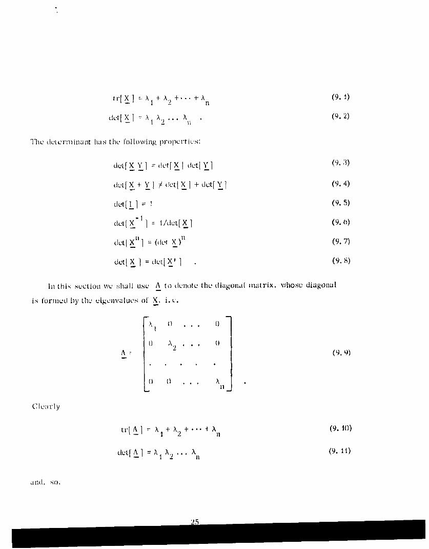
tr IX] 1 + A,.) + (9.4)
(let[XI A X.) ... I . (9.2)
The delt rilinalnt has the following pr()1l)rti(2.-:
det[ X Y 1 ,tf X 1 (1t[ Y ] (9. .3)
dutX + YJ / (let[X1 + dot[Yl (9.4)
det[I 1 1 (9.5)
ctet[ 1" 1 /d- eut[~ (_1 9. •)
det( X" 1 (,et x) (9.7)
deti X1 deut[X' 1 (9.8)
IlII this suction WLu ;lhall use. A to denotc thel diagonal matrix, Vhosc diagonal
is l'ormledLt by the Cig(AM'lLueS of X. i. L•-.
{} '\ 2( . .
A() A,)..,()A (9.9'))
C) 01 . .
C, I eI ny
tr . X1 A,+ + ... + A (9. IC)
~k..A] ~A . . A(9. 11)
and, .5on
25

tr[r _] = tr[ A_] (9. 12)
det[X] = det[Al. (9. 13)
Using the differential operator we have
d(tr[X 1) = d(tr[ A) (9. 14)
d(det[X]L) = d(det[ A]) . (9. 15)
Now we compute the differential of det[X] (provided X is nonsingular)
d(det[X1)= d(AA 2 "" 'N )
(dAI) Ak2 x... A + AI (dA2) A3... n
+ . ..X (dA )1 2 n-I 11
S ill + ... 2 4(9. 46A)
We note that we can identify
L~ I-- T tr[A d Al and, so,
1i=A•
in view of (9. 13) we have
-1d(det[XI) (dut[Xl) tr[ d Al (L).17)
26
\Ne H4lla 110 13mw JIUO t elot' I'1Vloing en ma11
l~eum Q 1I X i..' noml-in~glikirand;ili it' it da (istinct ciiýCi)ValiQs A A . x
ni- A- I 'k t X- (x I 9 8
P~roor: X anid A arc rclal ed hv th ;he i il arit v I raniisorI I]at ion
Ar 1) ' (9 1)
A 1 x P. (9. 20)
Fromu Eq. (L9. 19) wye have
P A X I (9. 2 1)
and. so,
(d 1) A + 11(d A)(LX )P +X (d P)) 9 22)
hi follows that
d A P(LiX) P + PX (OIP - P(dP) A *(9. 23)
Vrom l!qcs. (9. 12), (9. 20) a id (9. 23) Nve oI'toIii
A-1I tA - P)-x X- 11 p- I(X )P +P X 11 P1- X (odP) (0.24)
- -Pl pX I (dl) P- I P
1' X- (d) +l( P )-P X- ( 1) P X P,
27

1`lll'iiii ing Iu t roce (ft both sidCS alld LI~iflg'? the piropertics (2. 11) and (2. 12) we finid
t 11 dj A j IX] (Q. 25)
llsýiiig 1"(1s. (q. 18) and (9. 19) we arrive at'l
d(Ldet [ I) `(del[I[I1) tr[ dX ].(9.20)
We' C d~l llON% C0iriput ' the grladienlt. Ilatr'iX 01' det X ] i. v. the mlatrix
d~tjA(9. 27)
Ul0111 (Q. 20) we have
=dvt[X]j trtX,-IEi -1 (9. K) B
and, ,;cl, L'U1mm1a 8. 1 Yields
a ( [X] = (ldu [X). (X9)
If %vu write E~q. (9. 20) in the mUore silggestivc formn
-(ltliI tr[X -I x (9. 31)dLet [ X]
F~qimatlor (1). ?0) is true even if the cigenvaiues arc niot distinct; sece Rde. L7 35.

CC t 11 S iC' t~a
d(loig d Xl) r dX (.1
anid t hat
lo d 1 X (3 2)
(a mo st useful rcLiatioii). Usil](. 11 iIII-0' proeItV (W. .3) Of tI he det crn1i nalnt func tioln it i:.
.1vIo p row t hat
dct A BA I t (Xi-(0 3.3)
Als,4o, it i." CiiS'~ tO SI10W (ill ViLAN Of ( ) thaIt
Fro 1)UIlL ObI)Vmlts relatLion
d(LILut [ I q =to~e 11X 7, )'' kit [ ]) 1) d(dut X ) (9. 3s)
we2 cone Jude that 1,q. (9. 2o) y iclds
d(dut I):: i" (ddL [ 11)" tri x CA I 'i. o0)
dol (X1 ] (dutI, ) (x 1) 917)aJx _-

1t. PARTITIONED MA'TRICES
It is often necessary to work with partitioned matrices. Thu following formulae
3r% very useful.
Consider thu nx n matrix X partitioned as follows:
il 2
x ~x•
whe re
Xý is n i xnIi mutrix
- 1 1 1
-. 2 is n "< 11) -at rix
X is. 11 X~ n matrix
X s !. .. X n,( i1atrix
n +f 11 U. t
Assumv the necvs~sury invLrSe.S Cxisi. and that X_ is also partitioned as 111
((.I.Thun
+X x a X. x,,
- -I -X1 -il -it n12 n 1 a12r
X---------------------------------- :----------------------- o. 2)
-A X.) A
-_-22 -21 -nlmtix-1
X x_)x•2•_ Itxl -x12x1_
-30

lt'm1 (0t). 2), h c) If 1l0<wi jg is oht Iinild.
I +-I 1 - 0 -1
-th(ju f +) x x X X x )lo .1 oIu).-
t -- l etI -'-x I - 2 -2x2 -21-. -. 2 -2
it Y i al isa sil .d as in (il. 1), th..Ll1
x., A •.11+• . •. 1 2 x~Y X + 3 .,','.,.,(0.
+i]-iX 1 +i1[ 112] + U.7
x Y -- (o. 8)
L 1, +XY x Yt +X -22 1 12 +X22-!
L31

TABLE OF GRADIENTS
a
ax
ax
4. -L- tr[A XB] = A'B'
ax
0. 1-ti-[AX A
ax
" a thi-[ 13]~ = BA'
7u. _r[ _' A2 '
8
ox" --
a2. - "tr A _ l•-I A '1 '
-2- tr[ n(x )'
12. t'-r2", n I nA xl1
ax
7.~~ ~~ ~~ 2--~,[ xla.

TABILE O" GIR A•I) •,TS (Contincd)
) Xn~* Xi ~n- 1i13. Z- t"1 AX X
i=0
14. t-'•" [A L" 1B N 1 = A'X'1B + 1B'X'A'0X
15. --)-tr[AXI3X]' =A'X Fi' +AX1)
a X
16 - tr c j cax [t]
1-7 1 , -2L
axa -L - A -1
21. 1"ý ,t A _] .(dc A X )) (x )
1) -20. il"og d tet' x l X (X_. )
Ox
33

REFERENCES
1] F. C. Schwuppc, "Optimization of Signals,' Group Report 1904 -4, MITLincoln Laboratory (1904).
21 F. C.Schwulppe, "On the Distance Between Gaussian Processes: "'hle StateSpace Approach, " JA-26-39. MIT Lincoln Laboratory, 1965.
3 ] F. C. Schweppc. "Radar Frequency Modulations for Accelerating TargetsU nder a Bandwidth Constraint, " ILEE Trans. on Military blectronics,MIL-9, pp 25-32 (1965).
41] M. Athans and F. C. Schwepe., "On the Design of Optimal ModulationSchemes via Control Theoretic Concepts. I: FIormultation, " JA-263:4, MITLincoln Laboratory, 1905.
[ 5 ] N. Athans, "Solution of the Matrix Lquation A( () A(1) (t) + (t) l(t)+ U(t),
Technical Note 1905-220, MIT Lincoln Laboratory, Lexington, Mass., (1905).
0 F. C. Schweppc and D. Gray. "aLada Signal l)usign Subject to Sinultancousi'vok and AvcragQ Power Constraints, " JA-2559, MIT Lincoln Laboratory.to b),. published in IEtLE Trans. onl Information Theory,
7 1.. bodewig, Matrix CALkulus, North I loiland IPLiblLshilg Company andInter scicncc Publiishers, N. Y. , (1950),
[ R 1 . ielClmian, lilt roLIuct iol 10 Matrix Aiialysis, McGraw-H ill B~ook Co. , N.Y.(19o3).4
34.
Recommended
![s3-eu-west-1.amazonaws.com · Web viewSimulation Package (VASP) [1, 2]. The DFT calculations employed the Perdew, Burke, and Ernzerhof (PBE) [3] generalized gradient approximation](https://img.pdfslide.net/doc/110x75/5b03edff7f8b9a89208ce3c6/s3-eu-west-1-viewsimulation-package-vasp-1-2-the-dft-calculations-employed.jpg)