1

International Symposium “Steel Structures:Culture & Sustainability 2010” 21-23 September 2010, Istanbul, Turkey

Paper No: 14

GUIDELINES FOR MODELING THREE DIMENSIONAL STRUCTURAL CONNECTION MODELS USING FINITE ELEMENT METHODS

Serdar SELAMET1, Maria GARLOCK2

1�Graduate Student, Department of Civil and Environmental Engineering, Princeton University

2�Assistant Professor, Department of Civil and Environmental Engineering, Princeton University

ABSTRACT Simple shear (fin plate) connections, which are designed to resist shear loads only, are commonly used in the US. However, as observed in the Cardington large-scale building experiment, these connections carry large compressive forces during the heating phase of a fire that can lead to local buckling of the connecting members (i.e. beam). Further, large tensile forces develop near the connection during the fire decay which can lead to the failure of the connections. The objective of this research is to provide guidelines and address common problems to researchers in modeling three dimensional connection details using commercial finite element software such as ABAQUS. Modeling such FE models, which consists of several parts in contact, requires knowledge in contact mechanics with friction, meshing techniques, matrix solver and stability and convergence algorithms. In recent studies, researchers have made several attempts to model and run double angle (web cleat) or single plate connection models under a given fire load. A general consensus has been difficulty in setting up a proper contact surface configuration and overcoming rigid body motions and convergence problems related to contact and local buckling. With some examples from previous and ongoing research on simple shear connections at Princeton University, we aim to give suggestions on how to improve convergence characteristics of such models by selecting an optimum meshing level near contact areas, using stability methods and matrix solver techniques. Steel connections under fire events have been the least researched yet crucial area in the structural engineering and fire practice. Due to the high cost of conducting experiments of connections in a furnace, the finite element method is a cost-effective way to investigate the strength and behavior of connections under fire. We have observed that contact surfaces with edges or corners create convergence difficulties. Although using an explicit solver might look like a better alternative to an implicit solver for large models, the results from an explicitly solved solution could be unreliable and hence this technique requires careful attention by the user during post-processing. Since an implicit solver requires the balance of forces for each iteration, the results are inherently stable. Keywords: Finite Element, Contact, Implicit, Shear Connection, Steel, Guidelines.

INTRODUCTION The behavior of connections has become an important research field in predicting performance-based design for steel frames especially after many researchers realized a knowledge gap in estimating the behavior of steel structures under fire conditions. Highly non-linear behavior of steel under elevated temperatures coupled with large deflections, fire-induced forces and local instabilities in the fully or partially restrained beams make the finite element method (FE) a favorable choice in estimating the ultimate load capacity of steel subassemblies. Among the various types of connections, simple shear

2

connections are considered to be most vulnerable to fire scenarios because they are only designed for shear (gravity) loads and cannot fully resist the large axial forces in the beams and the rotational demand during fire. The objective of this research is to provide guidelines and address common problems to researchers in modeling three-dimensional connection details using commercial finite element software such as ABAQUS. Modeling such FE models, which consists of several parts in contact, requires knowledge in contact mechanics with friction, meshing techniques, matrix solver and stability and convergence algorithms. In previous research (Garlock and Selamet 2010, Selamet and Garlock 2010), we validated a single plate shear connection that is used in Cardington full-scale building tests (Lennon and Moore 2003). FE model of this connection provided us valuable insight in possible challenges that researchers from the same research area might encounter. We will first discuss about the previous benchmarks on three-dimensional finite element modeling of steel connections and then present our guidelines and supply several examples from our lap joint models or the single plate connection FE model from the Cardington test.

GUIDELINES IN CONNECTION MODELING

Previous Approach: Bursi and Jaspart (1997, 1998) have done extensive research on FE modeling of bolted end plate steel connections. Their research provided guidelines not only to end plate steel connections but also to all bolted steel connections. They suggested that 3D FE models are superior in estimating the connection capacity, which leads to a more realistic global behavior of steel members (i.e. beams, columns). Thick or thin shells are unable to produce acceptable results especially for the bolt behavior since bolts could have varying stresses through their thickness and shells cannot accurately capture such stress state. Due to the limited computing power a decade ago, simulating contact conditions between bolts, plates and beams in a connection was a grand challenge. Therefore, Bursi and Jaspart limited their focus on pre-loaded and not pre-loaded bolted endplate connections, which are at ambient temperature and loaded with monotonically increasing loading. Since the authors’ main concern was bending dominated problems at ambient temperature, they compared FE results to the experiments through moment-rotation diagrams. Overall, FE results compared well with the experiments in terms of the initial stiffness and the ultimate load capacity but they did not accurately capture the onset of yield strength on which Bursi and Jaspart commented as the lack of residual stress representation in the FE models. The authors also investigated discretization of the connection geometry, use of element types and analysis category (elastic or plastic), the effects of friction (due to contact) in tangential direction between connection parts (i.e. bolts, plates) as well as bolt pre-loading and prying force effects. Bursi and Jaspart recommended the use of 3D first-order (linear) hexahedron elements with incompatible modes (C3D8I) in ABAQUS. Linear elements are better for hyperbolic (plasticity) problems, in which the strain yield is discontinuous. Each of these elements has 13 additional degrees of freedom (DOF) to the existing 24 DOF, which provides superior performance in bending dominated problems without having shear locking behavior or zero energy modes. The authors also suggested using at least 3 elements through thickness of a section if the section’s behavior is bending dominated. They calibrated beam elements and used this assemblage to represent shear and bending behavior of the bolts. Moreover, they experimented with gap elements (as opposed to surface contact method) to simulate contact conditions. The beam assemblage method for the bolts and gap elements for contact conditions were utilized for the purpose of reducing the computational expense. The findings suggested that changing the Columb friction coefficient ȝ for tangential contact between bolts and end plate does not affect the rotational response of the end plate connection.

3

Van der Vegte and Makino (2004) investigated solution techniques to the structural problems involving bolted connections. He commented on the use of implicit and explicit solution schemes for such 3D FE connection models. Explicit method is usually used for dynamic problems because it determines the solution without iterating but by explicitly advancing the kinematic state from previous increment. Explicit problems do not need to form a global stiffness matrix because the linear equations are not solved simultaneously for the entire system (like in implicit method) but the stress wave propagates element-to-element (local). Implicit method steps in time by assembling global stiffness matrix for the entire structure and inverting it to find all nodal displacements. Hence, the user could experience high computational expense and converging difficulties since bolted connection models involving contact conditions are highly non-linear. Finally, the authors recommend using explicit solvers for large models with several parts in contact.

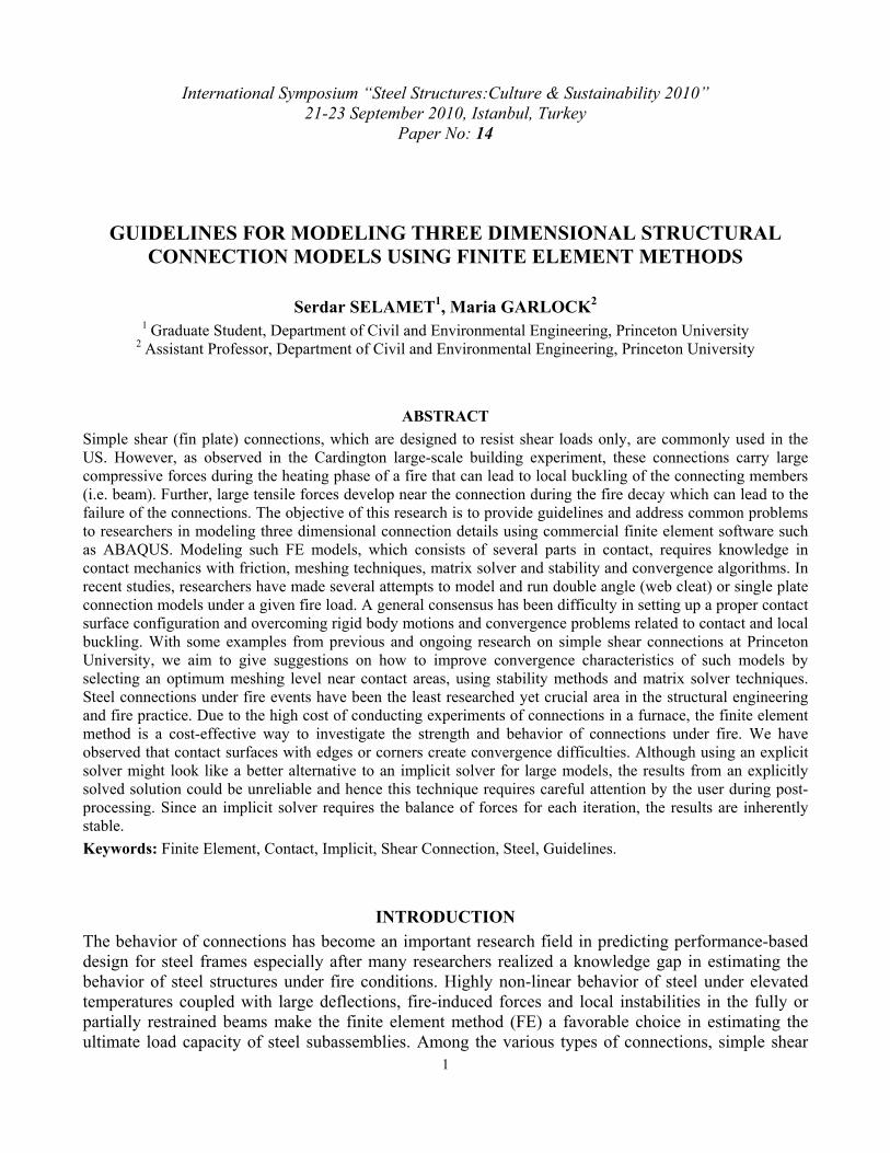
New and Enhanced Guidelines: Our paper expands and enhances this previous research in several directions. First, it investigates single bolt lap joints (tensile connections composed of 1 bolt and two plates) and simple shear connections in a subassembly. Previous research (Bursi and Jaspart 1998) focuses on isolated connections, which fail under monotonically increasing load. In our FE analyses, axial force, moment and shear develop simultaneously due to fire and imposed boundary conditions on the subassembly. Second, our paper considers highly nonlinear steel material behavior at elevated temperatures. Third, it uses state of the art solving techniques and contact configurations provided by the finite element software ABAQUS (DS-Simulia 2008). Element type and integration order: Whether the structure is at ambient temperature or under fire conditions, the FE models must be modeled for plastic problems if the goal is to estimate the ultimate load capacity (limit state). Hence, first-order elements should be used for bolted connection type problems in order to capture strain discontinuities (yield lines). Quadratic elements such as C3D20 are more accurate for elliptic (elastic) problems but they create additional difficulties when contact surfaces exist in the structure, because the shape function on element edges is not linear. However, it is inefficient to use only C3D8I elements for the entire model because each element has 13 additional DOF when compared to the fully integrated elements (C3D8). When the elements are not in the contact zone or not expected to have large stress concentrations, C3D8R (reduced integration) elements can be used to decrease the computational expense. They are not suited for contact zone because they are inherently rank deficient and can switch to zero energy modes. When these modes are triggered, the element can deform without any resistance to the load. C3D8 elements are generally more accurate than C3D8R elements, but they are subject to shear locking behavior, which can lead to overestimation of the load capacity in bending dominated problems. They can be used in parts of the structure where local stress concentration is high but no large bending is expected. The user should adopt hexahedron elements (C3D8, C3D8R and C3D8I) where possible. If the user needs to represent irregular geometry such as fillet radius of an I-Beam or a welded region, wedge elements (C3D6) can be used with care because the mesh density should be very fine in order to get acceptable stress results. Figure 1 shows how closely the FE model with C3D8I elements can capture (C3D8 elements overestimate the load capacity because of shear locking behavior) the load-displacement history of L8x5/8x4 angles (Garlock et al. 2003). The displacement is measured from the heel of the angle (uplift) and the force is measured from the thick plate that is connected to the angle through 4 bolts. For brevity, the load is applied for one cycle only until the deformation in the angle heel displaced by 1 inch. Since the angle in the experiment does not show any reduction in ultimate strength for each cycle until it fails by fatigue, the FE model is loaded only once.

FM

M

n

m

u

t

h

F

tp

(a) L8x5/8x4Figure 1. CoModel (C3D

Meshing anThe finite enumber of ecost of comstress concemeshed withThis numbeand Jaspart using 2 C3Dlocal bucklithickness. PC3D8I elemshown in Fihence we reand beam flaconnection rFigure 2 shocomplex mothickness. Tpractice anddisplacemenlimit state is

4 Angle omparison b

D8I Elements

nd steel matelement theoelements in t

mputation is aentrations exh 20 to 24 er is found by(1998). If t

D8 elementsing is a pos

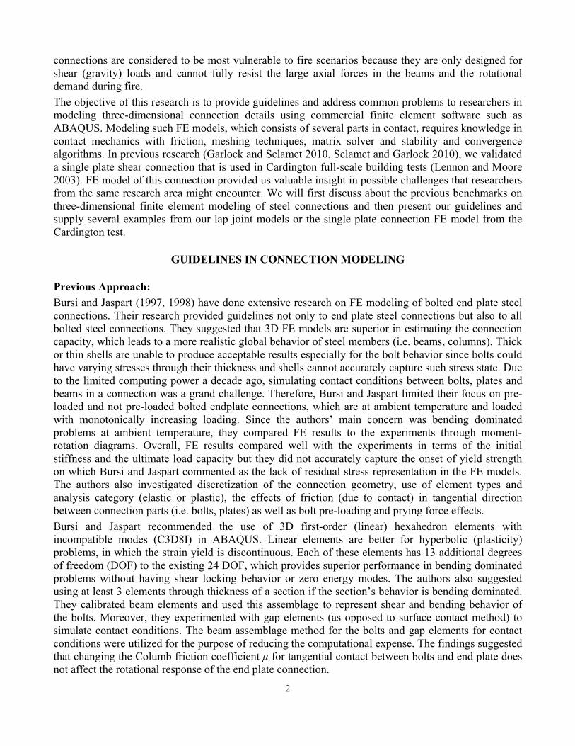
Post-bucklingments are suiigure 3a-b isecommend uange, the sinregion (for thows the simodels are buiThe bolt-holed will allow nt-controlleds reached (G

(b) Lobetween Exps).

terial propeory states ththat region galways a conxist near theelements aroy mesh convthe connectis through thessible conceg strength oitable for cos subjected tusing C3D8 ngle plate anhe rest of the

mplest tensileilt. The conne is 1/16’’ lathe bolt mov

d loading is aarlock and S

oad-Displacperimental C

rties: hat the numgets finer. Fncern, and ine connectionound the circvergence stuion is designe plate thickern and the f a plate de

onnections uo shear, comelements on

nd bolts in the subassembe connectionnection consarger than thve relative tapplied to thSelamet 2010

4

ement Plot fCyclic Loadin

merical modeor contact pntelligent mn, bolts, placumference

udies, which ned for tenskness. If the

user shouldpends on th

under comprempression, ten the contache connectionbly). n, which is usists of one bhe bolt diamto the two plhe other plat0).

for the Expeng Angle Te

el will convproblems, thi

meshing decisate- and beaof a typicalalso agree w

sile loadingconnection

d use at leahe bending bession. A simension and bt zones, C3Dn region and

used to validbolt (M20) c

meter (7/8’’). lates. The me until eithe

riment and Fest (Garlock

erge to the is also holdssions must bam bolt-holel bolt diamewell to the s(see Figure should alsost 3 elemen

behavior of mple single

bending throD8I element

d C3D8R ele

date the FE connected toThis is com

model is fixer bolt-hole b

FE model et al. 2003)

true solutios true. Howebe made. Sine regions sheter (7/8’’ tosuggestions b

2), we recoo resist compnts though tthe elementplate conne

oughout the ats for the be

ements outsid

model befoo 2 plates w

mmon in engd in one plabearing or bo

) and FE

on if the ever, the nce high hould be o 1 ¼’’). by Bursi ommend pression, the plate ts; hence ection as analysis, eam web de of the

ore more with 3/8’’ gineering ate and a olt shear

F

F

F

wmwpy

u

b

r

p

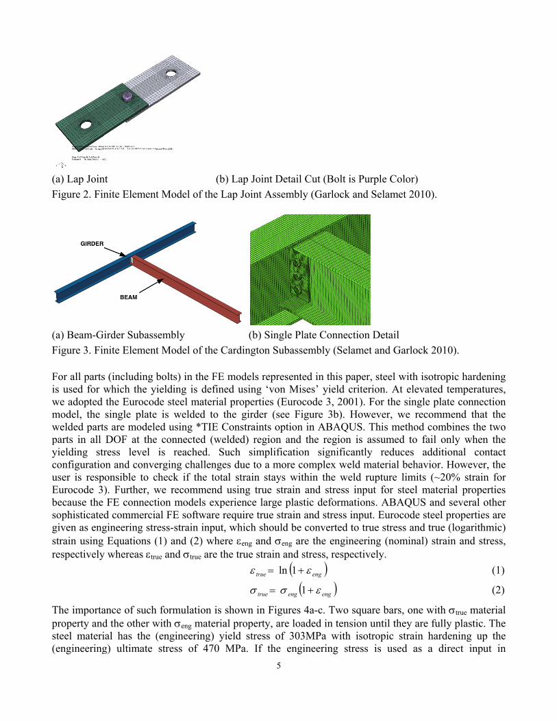
(a) Lap JoinFigure 2. Fin

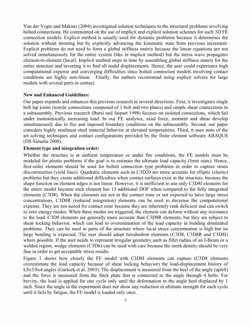
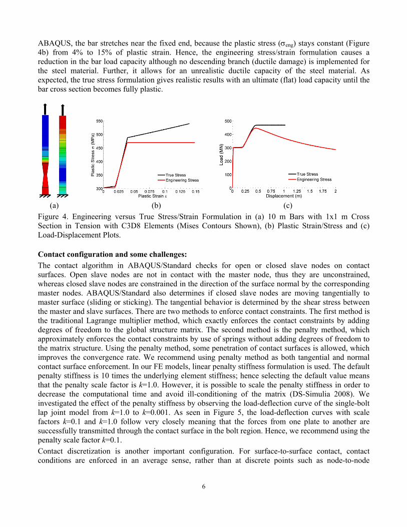
(a) Beam-GiFigure 3. Fin

For all partsis used for wwe adopted model, the welded partparts in all yielding strconfiguratiouser is respEurocode 3)because the sophisticatedgiven as engstrain using respectively

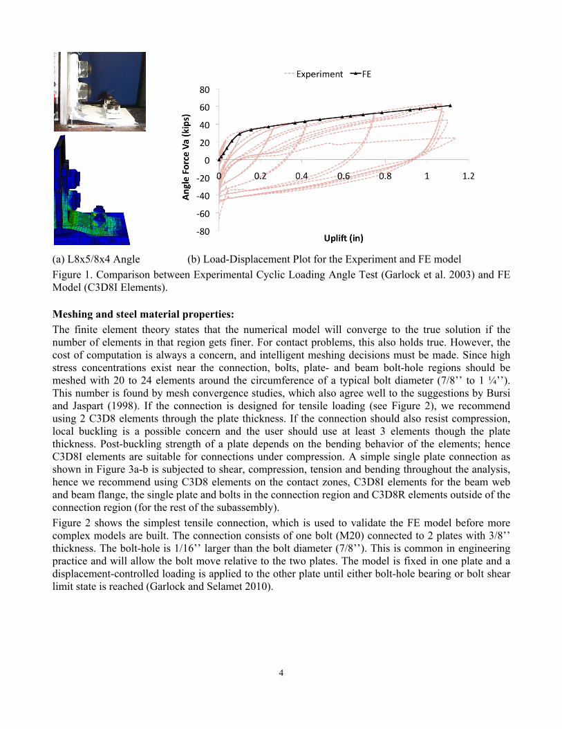
The importaproperty andsteel materi(engineering

nt nite Element

irder Subassnite Element

s (including bwhich the ythe Eurocodsingle plates are modeleDOF at theress level

on and conveonsible to c). Further, wFE connect

d commerciagineering strEquations (

y whereas Htru

ance of suchd the other wial has the (g) ultimate

t Model of th

sembly t Model of th

bolts) in theielding is dede steel matee is welded ed using *TI

e connected is reached

erging challecheck if the we recommetion models al FE softwaress-strain in(1) and (2) wue and Vtrue a

h formulationwith Veng mat(engineeringstress of 4

(b) Lap Johe Lap Joint

(b)

he Cardingto

FE models efined usingerial propertto the girdeIE Constrain(welded) re. Such simenges due tototal strain

end using trexperience l

are require trnput, which swhere Heng aare the true st

truH

trV

n is shown interial properg) yield stre70 MPa. If

5

int Detail Cut Assembly (

) Single Plateon Subassem

represented g ‘von Misesties (Eurocoer (see Figunts option inegion and thmplification o a more com

stays withinrue strain anlarge plasticrue strain anshould be cond Veng are train and str

� eue H� 1ln

�engrue V � 1

n Figures 4arty, are loadeess of 303Mf the engine

ut (Bolt is Pu(Garlock and

e Connectionmbly (Selame

in this papes’ yield critede 3, 2001).

ure 3b). Hown ABAQUS.he region is

significantlmplex weld mn the weld

nd stress inpc deformationd stress inpuonverted to tthe engineeress, respecti�eng

�engH�

a-c. Two squed in tension

MPa with isoeering stress

urple Color)d Selamet 20

n Detail et and Garlo

er, steel witherion. At ele. For the sinwever, we r This methoassumed to

ly reduces material behrupture limi

put for steelons. ABAQUut. Eurocodetrue stress anring (nominaively.

uare bars, onn until they aotropic strais is used a

) 010).

ock 2010).

h isotropic haevated tempegle plate conrecommend od combineso fail only w

additional havior. Howeits (~20% stl material prUS and severe steel propend true (logaal) strain an

ne with Vtrue

are fully plasin hardeningas a direct

ardening eratures, nnection that the

s the two when the

contact ever, the train for roperties ral other erties are arithmic) nd stress,

(1)

(2)

material stic. The g up the input in

6

ABAQUS, the bar stretches near the fixed end, because the plastic stress (Veng) stays constant (Figure 4b) from 4% to 15% of plastic strain. Hence, the engineering stress/strain formulation causes a reduction in the bar load capacity although no descending branch (ductile damage) is implemented for the steel material. Further, it allows for an unrealistic ductile capacity of the steel material. As expected, the true stress formulation gives realistic results with an ultimate (flat) load capacity until the bar cross section becomes fully plastic.

(a) (b) (c) Figure 4. Engineering versus True Stress/Strain Formulation in (a) 10 m Bars with 1x1 m Cross Section in Tension with C3D8 Elements (Mises Contours Shown), (b) Plastic Strain/Stress and (c) Load-Displacement Plots.

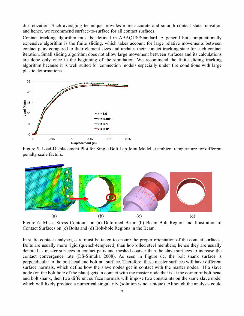
Contact configuration and some challenges: The contact algorithm in ABAQUS/Standard checks for open or closed slave nodes on contact surfaces. Open slave nodes are not in contact with the master node, thus they are unconstrained, whereas closed slave nodes are constrained in the direction of the surface normal by the corresponding master nodes. ABAQUS/Standard also determines if closed slave nodes are moving tangentially to master surface (sliding or sticking). The tangential behavior is determined by the shear stress between the master and slave surfaces. There are two methods to enforce contact constraints. The first method is the traditional Lagrange multiplier method, which exactly enforces the contact constraints by adding degrees of freedom to the global structure matrix. The second method is the penalty method, which approximately enforces the contact constraints by use of springs without adding degrees of freedom to the matrix structure. Using the penalty method, some penetration of contact surfaces is allowed, which improves the convergence rate. We recommend using penalty method as both tangential and normal contact surface enforcement. In our FE models, linear penalty stiffness formulation is used. The default penalty stiffness is 10 times the underlying element stiffness; hence selecting the default value means that the penalty scale factor is k=1.0. However, it is possible to scale the penalty stiffness in order to decrease the computational time and avoid ill-conditioning of the matrix (DS-Simulia 2008). We investigated the effect of the penalty stiffness by observing the load-deflection curve of the single-bolt lap joint model from k=1.0 to k=0.001. As seen in Figure 5, the load-deflection curves with scale factors k=0.1 and k=1.0 follow very closely meaning that the forces from one plate to another are successfully transmitted through the contact surface in the bolt region. Hence, we recommend using the penalty scale factor k=0.1. Contact discretization is another important configuration. For surface-to-surface contact, contact conditions are enforced in an average sense, rather than at discrete points such as node-to-node

p

Fp

F

B

p

n

w

discretizatioand hence, wContact tracexpensive acontact pairiteration. Smare done onalgorithm bplastic defor

Figure 5. Lopenalty scal

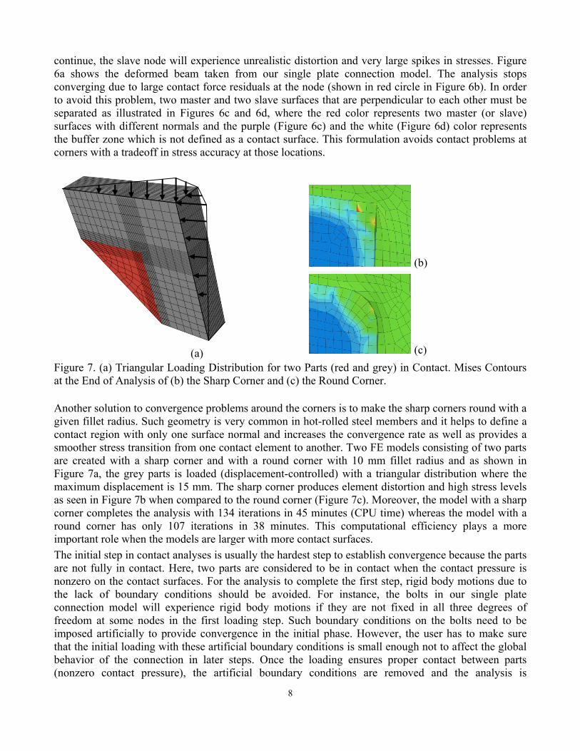
Figure 6. MContact Sur

In static conBolts are usdenoted as mcontact conperpendiculasurface normnode (on theand bolt shawhich will l

on. Such avewe recommecking algorialgorithm is s compared

mall sliding anly once in ecause it is rmations.

oad-Displacee factors.

(a) Mises Stress

faces on (c)

ntact analysesually more master surfanvergence raar to the bolmals, which e bolt hole oank, then twolikely produc

eraging techend surface-tithm must bthe finite slto their elem

algorithm dothe beginniwell suited

ement Plot fo

Contours oBolts and (d

es, care musrigid (quenc

aces in contaate (DS-Simlt head and b

define howf the plate) go different suce a numeric

hnique provito-surface fobe defined iliding, whicment sizes aoes not allowing of the sfor connect

for Single Bo

(b) on (a) Deford) Bolt-hole

st be taken tch-tempered)act pairs andmulia 2008)bolt nut surfa

w the slave ngets in contaurface normcal singulari

7

ides more acor all contactin ABAQUSh takes acco

and updates w large movsimulation. Wtion models

olt Lap Joint

(

rmed Beam Regions in t

to ensure the) than hot-ro

d meshed co). As seen ace. Therefonodes get inact with the m

mals will impity (solution

ccurate and t surfaces. S/Standard. ount for largtheir contac

vement betweWe recommespecially u

t Model at am

(c) (b) Beam B

the Beam.

e proper orieolled steel marser than thin Figure

ore, these man contact witmaster node

pose two conis not uniqu

smooth con

A general bge relative m

ct tracking steen surfaces

mend the finunder fire co

mbient temp

Bolt Region

entation of tmembers; henhe slave surf6c, the bol

aster surfaceth the mastethat is at the

nstraints on tue). Althoug

ntact state tr

but computamovements tate for eachs and its calcnite sliding onditions wi

perature for d

(d) n and Illustr

the contact snce they arefaces to incrlt shank su

es will have der nodes. Ife corner of bthe same slavgh the analys

ransition

ationally between

h contact culations tracking ith large

different

ration of

surfaces. e usually rease the urface is different f a slave bolt head ve node, sis could

8

continue, the slave node will experience unrealistic distortion and very large spikes in stresses. Figure 6a shows the deformed beam taken from our single plate connection model. The analysis stops converging due to large contact force residuals at the node (shown in red circle in Figure 6b). In order to avoid this problem, two master and two slave surfaces that are perpendicular to each other must be separated as illustrated in Figures 6c and 6d, where the red color represents two master (or slave) surfaces with different normals and the purple (Figure 6c) and the white (Figure 6d) color represents the buffer zone which is not defined as a contact surface. This formulation avoids contact problems at corners with a tradeoff in stress accuracy at those locations.

(a)

(b)

(c) Figure 7. (a) Triangular Loading Distribution for two Parts (red and grey) in Contact. Mises Contours at the End of Analysis of (b) the Sharp Corner and (c) the Round Corner.

Another solution to convergence problems around the corners is to make the sharp corners round with a given fillet radius. Such geometry is very common in hot-rolled steel members and it helps to define a contact region with only one surface normal and increases the convergence rate as well as provides a smoother stress transition from one contact element to another. Two FE models consisting of two parts are created with a sharp corner and with a round corner with 10 mm fillet radius and as shown in Figure 7a, the grey parts is loaded (displacement-controlled) with a triangular distribution where the maximum displacement is 15 mm. The sharp corner produces element distortion and high stress levels as seen in Figure 7b when compared to the round corner (Figure 7c). Moreover, the model with a sharp corner completes the analysis with 134 iterations in 45 minutes (CPU time) whereas the model with a round corner has only 107 iterations in 38 minutes. This computational efficiency plays a more important role when the models are larger with more contact surfaces. The initial step in contact analyses is usually the hardest step to establish convergence because the parts are not fully in contact. Here, two parts are considered to be in contact when the contact pressure is nonzero on the contact surfaces. For the analysis to complete the first step, rigid body motions due to the lack of boundary conditions should be avoided. For instance, the bolts in our single plate connection model will experience rigid body motions if they are not fixed in all three degrees of freedom at some nodes in the first loading step. Such boundary conditions on the bolts need to be imposed artificially to provide convergence in the initial phase. However, the user has to make sure that the initial loading with these artificial boundary conditions is small enough not to affect the global behavior of the connection in later steps. Once the loading ensures proper contact between parts (nonzero contact pressure), the artificial boundary conditions are removed and the analysis is

9

continued. Furthermore, we recommend that the small loading in the initial step should be displacement-controlled instead of force-controlled since they provide a higher numerical stability to the system. Solving techniques: Solving large FE models with high nonlinearity involving contact is a crucial issue for most researchers. Van der Wegte (2004) recommended explicit integration in time for connection models for ease with contact configuration and convergence. However, he warned the users to carefully analyze and interpret results. Explicit time integration is advantageous for large non-linear dynamic problems, for which inertial effects are important and the time of simulation is measured in milliseconds. However, 3D connection modeling at ambient or elevated temperatures is essentially a static problem. Explicit methods could be used quasi-statically for connection modeling under ambient or elevated temperatures, where the system produces kinetic energy (inertial forces) but this energy stays below a certain threshold (~10%) when compared to the internal energy of the system throughout the simulation. Explicit problems are also conditionally stable, because the stress wave propagation cannot exceed the smallest element size (critical element characteristic length). Hence, the stable time increment (ǻcr) is usually very small (refer Table 1) for finely meshed models. Using very small ǻcr makes it impossible to use a real time scale for quasi-static problems in Explicit method; instead a total time (ttotal) 0.005 seconds is selected (usually 10-50 times larger than ǻcr) such that the analysis completes faster, but the noise due to contact and the kinetic energy in the system are kept minimal. Implicit method does not have a time instability issue, but its computational expense grows almost exponentially with larger degrees of freedom and it inherently creates convergence problems when contact surfaces and high nonlinear materials are used in the model. We have included in Table 1 an example of the single bolt lap joint model (shown in Figure 2a) to compare explicit and implicit solution techniques.

Table 1. Implicit versus Explicit method of Single Bolt Lap Joint Model (see Figure 2a) using 64-bit System with Intel Xeon E5345, 2.33GHz, Quad-core CPU (parallel processing), 32 GB of RAM.

Parameters IMPLICIT EXPLICIT

Number of DOF / number of iterations 104262 / 735 79158 / 207165

Contact Enforcement Penalty method Penalty method

Computational Expense (CPU time / Memory) 3.93 hrs / 565 MB 2.16 hrs / 136 MB

Stable time increment (ǻcr) N/A 1x10-7 sec

Total time (ttotal) 1.0 (time is irrelevant) 0.005 sec

Analysis End (Bearing of the Bolt-hole) Field equations do not converge due to plastic failure.

The ratio of deformation speed to wave speed exceeds 1.0 for most elements.

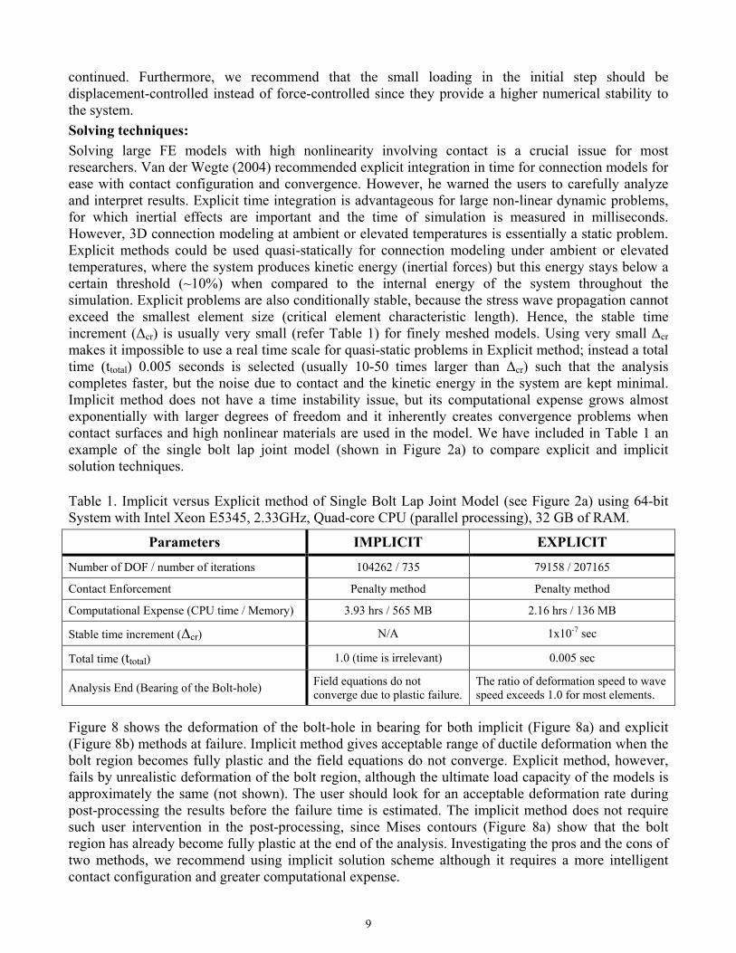
Figure 8 shows the deformation of the bolt-hole in bearing for both implicit (Figure 8a) and explicit (Figure 8b) methods at failure. Implicit method gives acceptable range of ductile deformation when the bolt region becomes fully plastic and the field equations do not converge. Explicit method, however, fails by unrealistic deformation of the bolt region, although the ultimate load capacity of the models is approximately the same (not shown). The user should look for an acceptable deformation rate during post-processing the results before the failure time is estimated. The implicit method does not require such user intervention in the post-processing, since Mises contours (Figure 8a) show that the bolt region has already become fully plastic at the end of the analysis. Investigating the pros and the cons of two methods, we recommend using implicit solution scheme although it requires a more intelligent contact configuration and greater computational expense.

10

(a) (b) Figure 8. Mises Contour and Deformation Plots of Single Bolt Lap Joint Models (ambient temperature) with Bolt-hole Bearing Limit State using (a) Implicit Method and (b) Explicit Method.

CONCLUSION Finite element software has evolved in the last decade to enable the researchers to implement 3D topologies such as connections with user friendly graphical support. The researchers still need to understand and overcome some of the difficulties that such models produce. In this paper, we discussed about previous principles for FE modeling of connections and developed more recent and comprehensive guidelines for connections under ambient or elevated temperatures in a subassembly. We also supported our recommendations with original examples such as lap joints or single plate shear connection from Cardington tests.

Acknowledgement This research is supported by the National Science Foundation (NSF) under grant number CMMI 0756488. All opinions, findings and conclusions expressed in this paper are the authors' and do not necessarily reflect the policies and views of NSF. The writers are grateful to Professor Panos Papadopoulos (Department of Mechanical Engineering, University of California at Berkeley) for his assistance with the ABAQUS and developing the finite element model.

REFERENCES DS-Simulia, ABAQUS, version 6.8 (2008), Documentation, Providence, RI. Bursi, O.S., Jaspart, J.P. (1997), Benchmarks for Finite Element Modelling of Bolted Steel Connections, Journal of Constructional Steel Research, 43 (1-3), 17-42. Bursi, O.S., Jaspart, J.P. (1997), Calibration of a Finite Element Model for Isolated Bolted End-plate Steel Connections, Journal of Constructional Steel Research, 44 (3), 225-262. Bursi, O.S., Jaspart, J.P. (1998), Basic Issues in the Finite Element Simulation of Extended End-plate Connections, Computers and Structures, 69 (3), 361-382. Eurocode 3 (2001), Design of steel structures Part 1.2: General rules structural fire design ENV 1993-1- 2:2001, European Committee for Standardization, Brussels, Belgium. Garlock, M.M., Ricles, J.M., and Sause, R. (2003), Cyclic Load Tests and Analysis of Bolted Top-and-Seat Angle Connections, Journal of Structural Engineering, 129(12), 2003, 1615-1625. Garlock, M.E., Selamet, S. (2010), Modeling and Behavior of Steel Plate Connections Subject to Various Fire Scenarios, Journal of Structural Engineering, accepted for publication for July 2010. Selamet, S., Garlock, M.E. (2010), Robust Fire Design of Single Plate Steel Connections, Engineering Structures, accepted for publication. Van der Vegte, G.J., Makino, Y. (2004), Numerical Simulation of Bolted Connections: The Implicit versus the Explicit Approach, AISC-ECCS, Amsterdam, Netherlands.