1
Machine Learning
Hauptseminar für Informatiker:Single-layer neural networks
Referent: Matthias SeidlBetreuer: Martin Bauer
09.12.2003

2
Overview
● Introduction
● Basic characteristics
● Linear separability
● Leastsquares techniques
● Perceptron
● Conclusion

3
The biological neuron

4
The artificial neuron
●
– Inputs: , .... ,
– Weights: , ... ,
– Bias: or threshold:
w1 w d
x1 x d
w0−w0
5
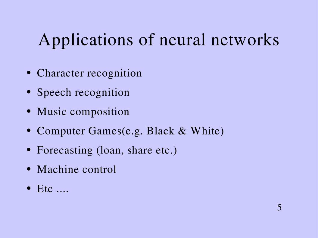
Applications of neural networks
● Character recognition
● Speech recognition
● Music composition
● Computer Games(e.g. Black & White)
● Forecasting (loan, share etc.)
● Machine control
● Etc ....

6
Network structures
● Feedforward networks vs Recurrent networks
● Singlelayer vs. Multilayer networks
● Supervised vs. Unsupervised
● Continous vs. Binary

7
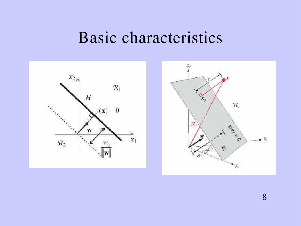
Basic characteristics(1)
● Two Classes: & – Linear discriminant:
– Linear dicision boundary: y(x) = 0corresponds to (d1)dimensional hyperplane in ddimensional xspace
– W defines orientation of decision boudary
– Normal distance from the origin to the hyperplane
y x = wT xw 0
wT⋅x∥w∥
=−w 0
∥w∥
C1 C2
8
Basic characteristics

9
Basic Characteristics● Several Classes: ,...,
– Linear discriminant:
– Distance of the decision boundary of the origin:
– Leads to a set of decision regions, which are connected and convex
y k x = w kT xw k 0
l=−w k 0−w j 0
∥ w k− w j∥
C1 C c

10
Activation functions
● Activation function
– Step (Threshold) function
– Linear functions
– Logistic Sigmoid (=>next slide)
y x =g wT xw 0

11
Activation functions
● Logistic sigmoid–
– sshaped
– Monotonically increasing
– Differentiable
– Maps auf (0,1)
– Output of network in a limited range
−∞ ,∞

12
Logistic Regression
● Motivation for logistic sigmoid: normal distributions with equal covariance matrices
● From Bayes Theorem we have:
mit
● Outputs of neural network can be interpreted as posterior probabilities

13
Logistic Regression
● After substituting expression for gaussdistribution in expression of BayesTheorem we obtain
mit
● => results: next slide

14
Logistic Regression
● Outputs of neural networks can be interpreteted as posterior probabilities
● Procedure to estimate the weights

15
Logistic Regression
● Binary Input Vectors– Leads to Bernoulli distribution
● => Outputs of neural Networks can be interpreted as posterior probabilities
px∣C k =∏ i=1
dP kix i 1−P ki
1− x i

16
Linear Separability
● Definition: If all points of training data is correctly classified by a linear(hyperplanar) decision boundary, then the points are said to be linerarly separable.
● Examples: OR, AND ● Contraexample: XOR, NXOR

17
Linear Separability
● What fraction of dichtomies is linearly separable?
● Distribute N data points in K dimensions in general position
● Assign the points randomly to Classes or
● Binary inputs pattern hence assignments to the two classes. Less than can be implemented by a perceptron and are called treshold logic functions.
=> solution: generalized linear diskriminants
C1 C2
2K 22K
22K /K !

18
Leastsquares techniques
● Sumof sqaures error function
– :Represents output of unit k
– : target value for output of unit k
– N : Number of trainig pattern
– C : Number of outputs
E w=12∑n= 1
N
∑k= 1
c y k x
n ; w−t kn2
yk x n
t kn
19
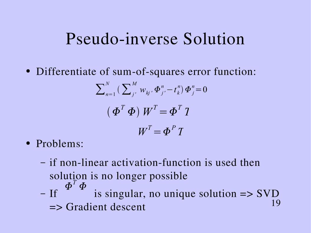
Pseudoinverse Solution
● Differentiate of sumofsquares error function:
● Problems:
– if nonlinear activationfunction is used then solution is no longer possible
– If is singular, no unique solution => SVD=> Gradient descent
∑n=1
N∑ j '
Mwkj ' j '
n −t kn j
n=0
T W T=T T
W T=PT
T

20
Gradient Descent

21
Gradient Descent
● For GLN partial differntial is:
● Leads to delta rule: ● Gradient Descent for logistic sigmoid
– Derivatives of error function:in which:
– The derivative of logistic sigmoid can easily be expressed in the simple form:
∂ E n ∂wkj
=[ yk xn−t k
n] j xn=k
n jn
wkj=−kn j
n
∂ E n ∂wkj
=g ' ak kn j
n
kn= g ' ak yk x
n−t kn
g ' a= g a1− g a

22
Gradient Descent Algorithm
● Initialise weights to random values● Iterate through a number of epochs. On each
epoch do:– Run each case through the network, so that the
output is produced. Calculate the difference (delta) between the output and the target values. Use this with gradient descent rule to adjust the weights.
– When deltarule becomes almost zero, stop.
wkjt1=wkj
t −kn j
n
23
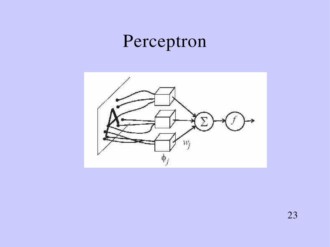
Perceptron
24
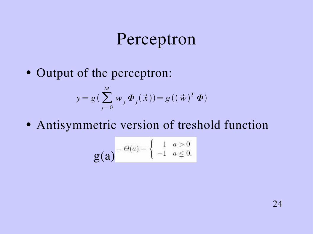
Perceptron
● Output of the perceptron:
● Antisymmetric version of treshold function
g(a)
y=g∑j= 0
M
w j j x =g wT

25
Perceptron
● The perceptron criterion:
● Perceptron learning:
● Perceptron convergence theorem: For any data set which is linearly separable, the perceptron learning rule is garanteed to find an solution in a finite number of steps
E perc w=− ∑n∈M
wT n t n
w jr1=w j
r jn t n

26
Perceptron
● Applet for Perceptron learning:http://home.cc.umanitoba.ca/~umcorbe9/perceptron.html
● Limitations(Minsky, Pappert)– Diameterlimited perceptron

27
Pros & Cons of singlelayer networks
● + simple learning algorithm
● + can solve problems quite readily
● + Insentivity to (moderate) noise or unreliability in data
● + Ability to have more output classes
● only a small class of problems can be classified correctly (XOR)
● black box (difficulties in validation the model)

28
Conclusion
● Single layer neuralnetworks which form a weighted biased sum of their inputs implement a linear discrimant
● Output of logistic sigmoid network can be interpreted as posterior probabilities
● Can optimize weights using Pseudoinverse and Gradient descent

29
Literature
● Christopher M. Bishop Neural Networks for Pattern Recognition” Chapter 3.1.3.5. , Clarendon Press Oxford, 1995
● Stuart Russell, Peter Norvig „ Artificial Intelligence – A modern approach“ Chapter 20.5, Prentice Hall, 2003
● David J.C. MacKay „ Information Theory, Inference, and Learning Algorithms“ Chapter 3841, Cambridge University Press
● Online literature:– ftp://ftp.sas.com/pub/neural/FAQ.html
– http://home.cc.umanitoba.ca/~umcorbe9/neuron.html
– http://www.aijunkie.com/nnt1.html
– http://neuralnetworks.aidepot.com/
Recommended