Li DengMicrosoft ResearchUW-EE516; Lecture May 21, 2009
Hidden Markov Models, Discriminative Training, and Modern Speech Recognition

Architecture of a speech Architecture of a speech recognition systemrecognition system
Application
Voice
Application
Signal Processing
Acoustic
Models
Decoder
Adaptation
LanguageM
odels

Fundamental Equation of Speech Fundamental Equation of Speech RecognitionRecognition
Roles of acoustic modeling and Hidden Markov Model (HMM)
ˆ arg max ( | ) arg max ( | ) ( )W W
W P W x P x W P W= =

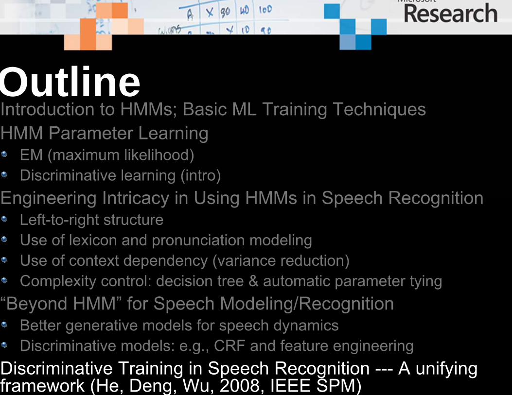
OutlineIntroduction to HMMs; Basic ML Training TechniquesHMM Parameter Learning
EM (maximum likelihood)Discriminative learning (intro)
Engineering Intricacy in Using HMMs in Speech RecognitionLeft-to-right structureUse of lexicon and pronunciation modelingUse of context dependency (variance reduction)Complexity control: decision tree & automatic parameter tying
“Beyond HMM” for Speech Modeling/RecognitionBetter generative models for speech dynamicsDiscriminative models: e.g., CRF and feature engineering
Discriminative Training in Speech Recognition --- A unifying framework

HMM Introduction:Description
• The 1-coin model is observable becausethe output sequencecan be mapped to a specific sequence ostate transitions
• The remaining modeare hidden because the underlying state sequence cannot bedirectly inferred fromthe output sequence

Specification of an HMMA - the state transition probability matrix
aij = P(qt+1 = j|qt = i)B- observation probability distribution
bj(k) = P(ot = k|qt = j) i ≤ k ≤ Mπ - the initial state distribution
Description
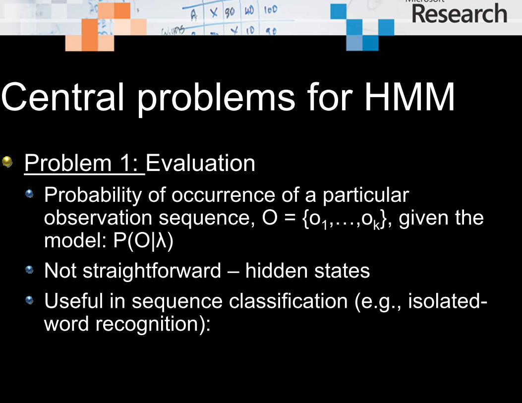
Central problems for HMMProblem 1: Evaluation
Probability of occurrence of a particular observation sequence, O = {o1,…,ok}, given the model: P(O|λ)Not straightforward – hidden statesUseful in sequence classification (e.g., isolated-word recognition):
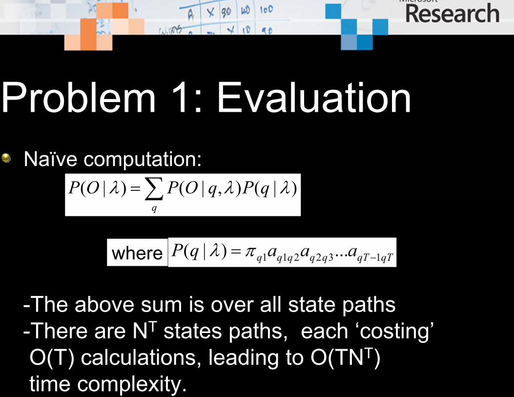
Problem 1: EvaluationNaïve computation:
∑=q
qPqOPOP )|(),|()|( λλλ
-The above sum is over all state paths-There are NT states paths, each ‘costing’O(T) calculations, leading to O(TNT)time complexity.
qTqTqqqqq aaaqP 132211 ...)|( −= πλwhere

Problem 1Need efficient SolutionDefine auxiliary forward variable α:
),|,...,()( 1 λα iqooPi ttt ==
αt(i) is the probability of observing a partial sequence ofobservables o1,…ot such that at time t, state qt=i
1( ) ( ,..., | , )t t ti P o o q iα λ= =
),|,...,()( 1 λα iqooPi ttt ==),|,...,()( 1 λα iqooPi ttt ==
Then recursion on α provides the most efficient solution to problem 1 (forward algorithm)

Central problems for HMMProblem 2: Decoding
Optimal state sequence to produce given observations, O = {o1,…,ok}, given modelOptimality criterionUseful in recognition problems (e.g., continuous speech recognition

Problem 2: DecodingRecursion:
Termination:
Backtracking:
)())((max)( 11 tjijtNit obaij −≤≤= δδ
))((maxarg)( 11 ijtNit aij −≤≤= δψ
NjTt ≤≤≤≤ 1,2)(max
1iP TNi
δ≤≤
=∗
)(maxarg1
iq TNiT δ≤≤
∗ =
P* gives the state-optimised probability
Q* is the optimal state sequence(Q* = {q1*,q2*,…,qT*})
)( 11∗∗ = qq ψ
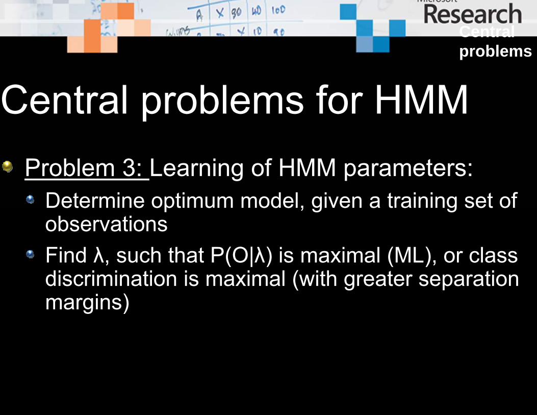
Central problems for HMMProblem 3: Learning of HMM parameters:
Determine optimum model, given a training set of observationsFind λ, such that P(O|λ) is maximal (ML), or class discrimination is maximal (with greater separation margins)
Centralproblems
OutlineIntroduction to HMMs; Basic ML TechniquesHMM Parameter Learning
EM (maximum likelihood)Discriminative learning
Engineering Intricacy in Using HMMs (Speech)Left-to-right structureUse of lexicon and pronunciation modelingUse of context dependency (variance reduction)Complexity control: decision tree & automatic parameter tying
“Beyond HMM” for Speech Modeling/RecognitionBetter generative models for speech dynamicsDiscriminative models: e.g., CRF and feature engineering
Discriminative Training in Speech Recognition --- Aunifying framework
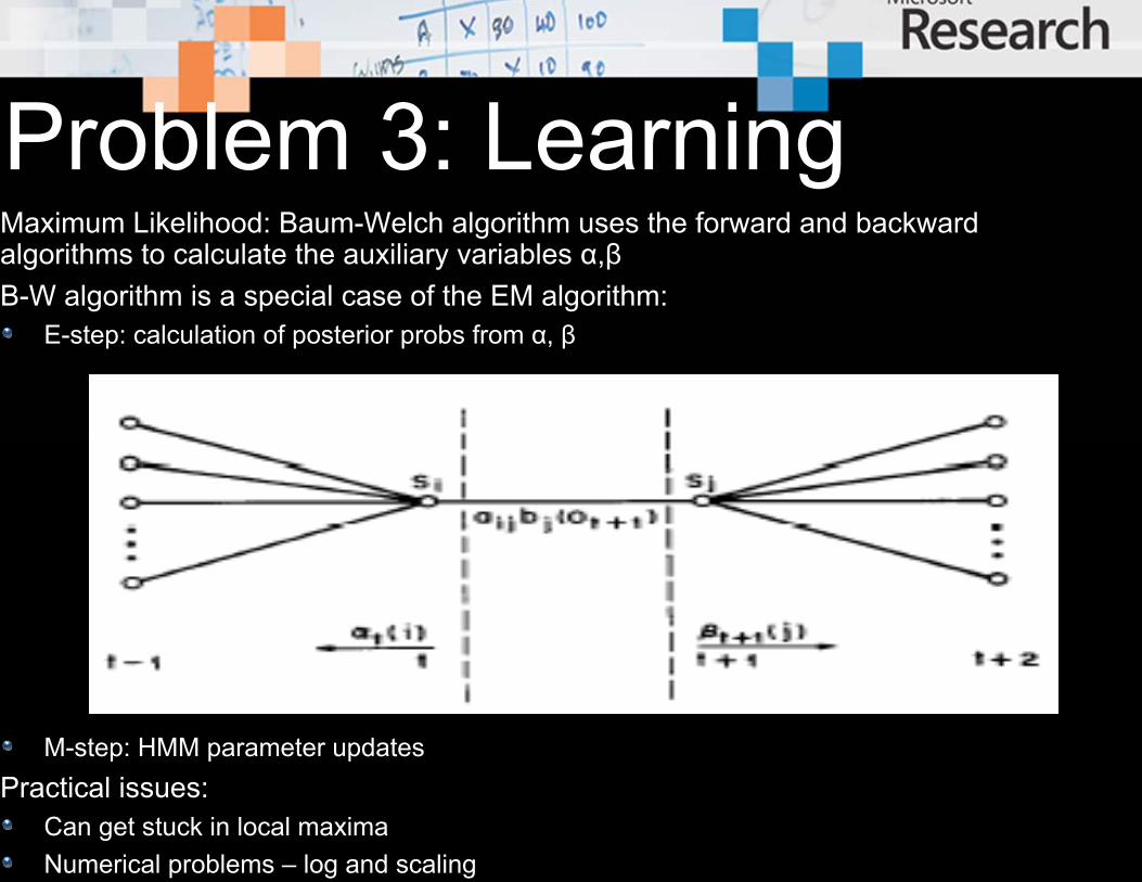
Problem 3: LearningMaximum Likelihood: Baum-Welch algorithm uses the forward and backward algorithms to calculate the auxiliary variables α,βB-W algorithm is a special case of the EM algorithm:
E-step: calculation of posterior probs from α, β
M-step: HMM parameter updatesPractical issues:
Can get stuck in local maximaNumerical problems – log and scaling
π ija )(ˆ kbj

Discriminative Learning (intro)Maximum Mutual Information (MMI)Minimum Classification Error (MCE)Minimum Phone/Word Errors (MPE, MWE)Large-Margin Discriminative TrainingMore Coverage later

OutlineIntroduction to HMMs; Basic ML TechniquesHMM Parameter Learning (Advanced ML Techniques)
EM (maximum likelihood)Discriminative learning
Engineering Intricacy in Using HMMs (Speech)Left-to-right structureUse of lexicon and pronunciation modelingUse of context dependency (variance reduction)Complexity control: decision tree & automatic parameter tying
“Beyond HMM” for Speech Modeling/RecognitionBetter generative models for speech dynamicsDiscriminative models: e.g., CRF and feature engineering
Discriminative Training in Speech Recognition --- A unifying framework
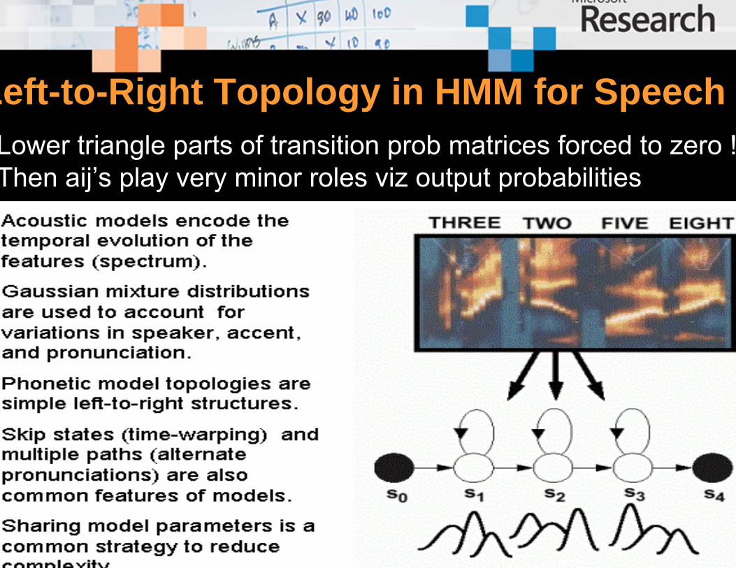
Left-to-Right Topology in HMM for SpeechLower triangle parts of transition prob matrices forced to zero !Then aij’s play very minor roles viz output probabilities

Word/Phone as HMM States, Lexicon, Context Dependency, & Decision Tree

OutlineIntroduction to HMMs; Basic ML TechniquesHMM Parameter Learning (Advanced ML Techniques)
EM (maximum likelihood)Discriminative learningLarge-margin discriminative learning
Engineering Intricacy in Using HMMs (Speech)Left-to-right structureUse of lexicon and pronunciation modelingUse of context dependency (variance reduction)Complexity control: decision tree & automatic parameter tying
“Beyond HMM” for Speech Modeling/RecognitionBetter generative models for speech dynamicsDiscriminative models: e.g., CRF and feature engineering
Discriminative Training in Speech Recognition --- Aunifying framework

HMM is a Poor Model for Speech (not just IID)

Major Research Directions in the Field
Direction 1: “Beyond HMM” Generative Modelingbuild more accurate statistical speech models than HMMIncorporate key insights from human speech processing

speech acoustics
motor/articulators
brain
messageInternalmodel
ear
brain
auditory rec
eption
SPEAKER LISTENER
decodmessa

Hidden Dynamic Model --- Graphical Model Representation
)1(1S )1(
2S )1(3S
)1(4S
)1(TS.......
)2(1S )2(
2S)2(
3S )2(4S )2(
TS.......
)(1
LS )(2
LS)(
3LS )(
4LS )(L
TS.......
....... .......
1t 2t 3t Kt4t
1z 2z 3z Kz4z
1o 2o 3o Ko4o
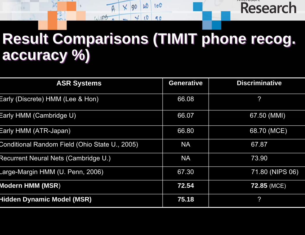
Result Comparisons (TIMIT phone recog. accuracy %)Result Comparisons (TIMIT phone recog. accuracy %)
ASR Systems Generative Discriminative
Early (Discrete) HMM (Lee & Hon) 66.08 ?
Early HMM (Cambridge U) 66.07 67.50 (MMI)
Early HMM (ATR-Japan) 66.80 68.70 (MCE)
Conditional Random Field (Ohio State U., 2005) NA 67.87
Recurrent Neural Nets (Cambridge U.) NA 73.90
Large-Margin HMM (U. Penn, 2006) 67.30 71.80 (NIPS 06)
Modern HMM (MSR) 72.54 72.85 (MCE)
Hidden Dynamic Model (MSR) 75.18 ?

Major Research Directions in the Field
Direction 2: Discriminative Modeling/LearningAcknowledge accurate speech modeling is too hardView HMM not as a generative model but as discriminant functionLarge-margin discriminative parameter learning“Direct” models for speech-class discrimination: e.g., MEMM, CRF; feature engineering; deep learning and structureDiscriminative training for generative models
OutlineIntroduction to HMMs; Basic ML Training TechniquesHMM Parameter Learning
EM (maximum likelihood)Discriminative learning (intro)
Engineering Intricacy in Using HMMs in Speech RecognitionLeft-to-right structureUse of lexicon and pronunciation modelingUse of context dependency (variance reduction)Complexity control: decision tree & automatic parameter tying
“Beyond HMM” for Speech Modeling/RecognitionBetter generative models for speech dynamicsDiscriminative models: e.g., CRF and feature engineering
Discriminative Training in Speech Recognition --- A unifying framework (He, Deng, Wu, 2008, IEEE SPM)

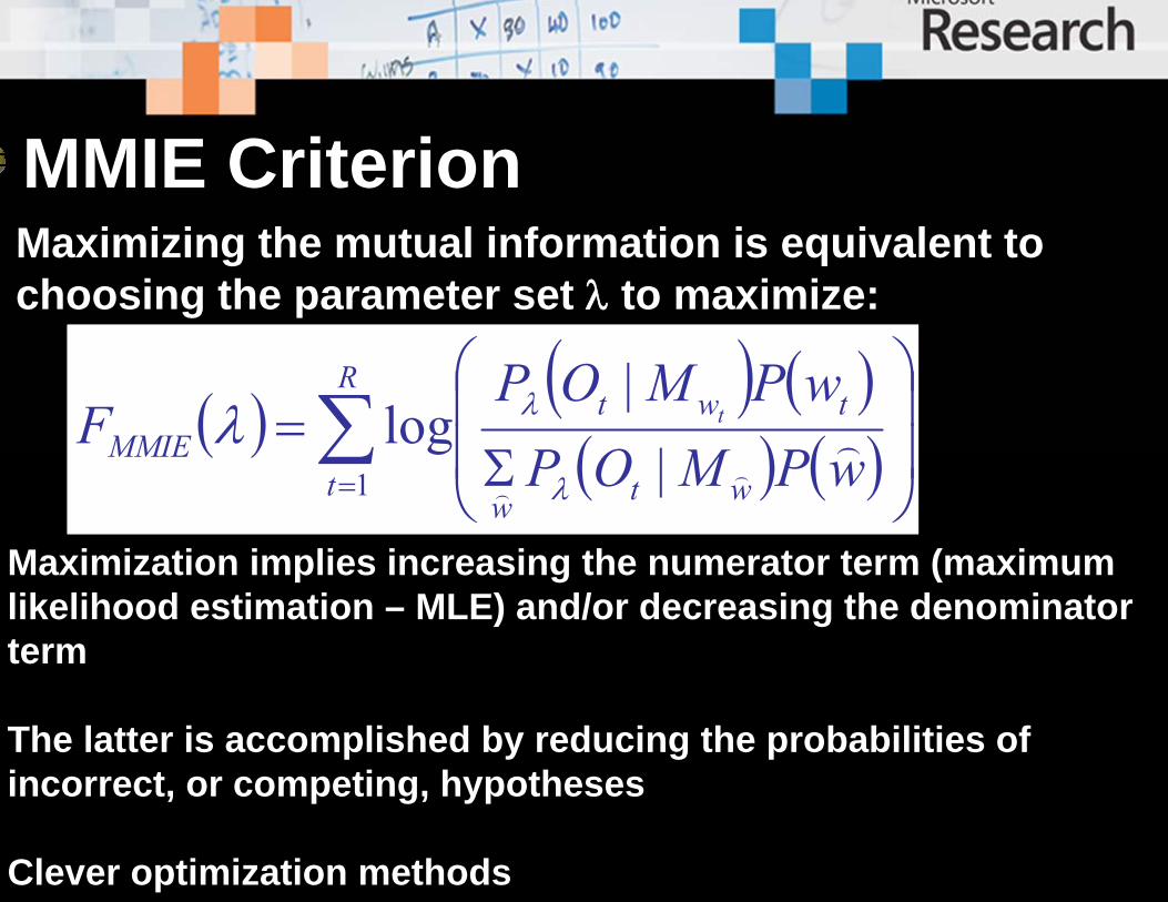
MMIE CriterionMaximizing the mutual information is equivalent to choosing the parameter set λ to maximize:
( ) ( ) ( )( ) ( )∑
=⎟⎟
⎠
⎞
⎜⎜
⎝
⎛
Σ=
R
t wtw
twtMMIE wPMOP
wPMOPF t
1 ||
logλ
λλ
Maximization implies increasing the numerator term (maximum likelihood estimation – MLE) and/or decreasing the denominator term
The latter is accomplished by reducing the probabilities of incorrect, or competing, hypotheses
Clever optimization methods

MPE/MWE Criteria
r
r
R s r r r 1 r rMWE
r=1 s r r r
p(X |s ,Λ) P(s ) A (s ,S )O (Λ)= p(X |s ,Λ) P(s )
∑∑
∑
•Raw phone or word accuracy A(s, S) (Povey et. al. 2002)•Requiring use of lattices to determine A(s,S)•Very difficult to optimize wrt HMM parameters•Engineering tricks•Unifying MPE, MCE, MMI (He & Deng, 2007) in both criterion and optimization method

MCE CriterionMiXg i ,1),,( =Λiscriminative functions:
),(maxarg),(),(,1,
Λ+Λ−=Λ=≠
XgXgXd jMjij
ii
[ ]
)(minarg
)()),(()),(()(
)(1),(),(1
Λ=Λ
∂⋅Λ=Λ=Λ
∈⋅Λ=Λ
Λ
=
∫
∑
L
XXPXdlXdlEL
CXXdXd
opt
XX
M
iii
Smoothed classificationError count:
Misclassification measure:
Optimization (gradient):
0,)))((exp(1
1)),(( >+Λ⋅−+
=Λ γθγ Xd
Xdli
i
here error smoothing nction is sigmoidal :

arge-Margin EstimatesMMI, MPE/MWE, & common MCE do not embrace margins“Margin” parameter m>0 in MCE’s error smoothing function
1( ( , )) , 01 exp( ( ( , ) ( )))i
i
l d Xd X m I
γγ
Λ = >+ − ⋅ Λ +
Careful exploitation of the “margin” parameter in LM-MCE training of HMM parameters leads to significant ASR performance improvement (Yu, Deng, He, Acero, 2006, 2007)
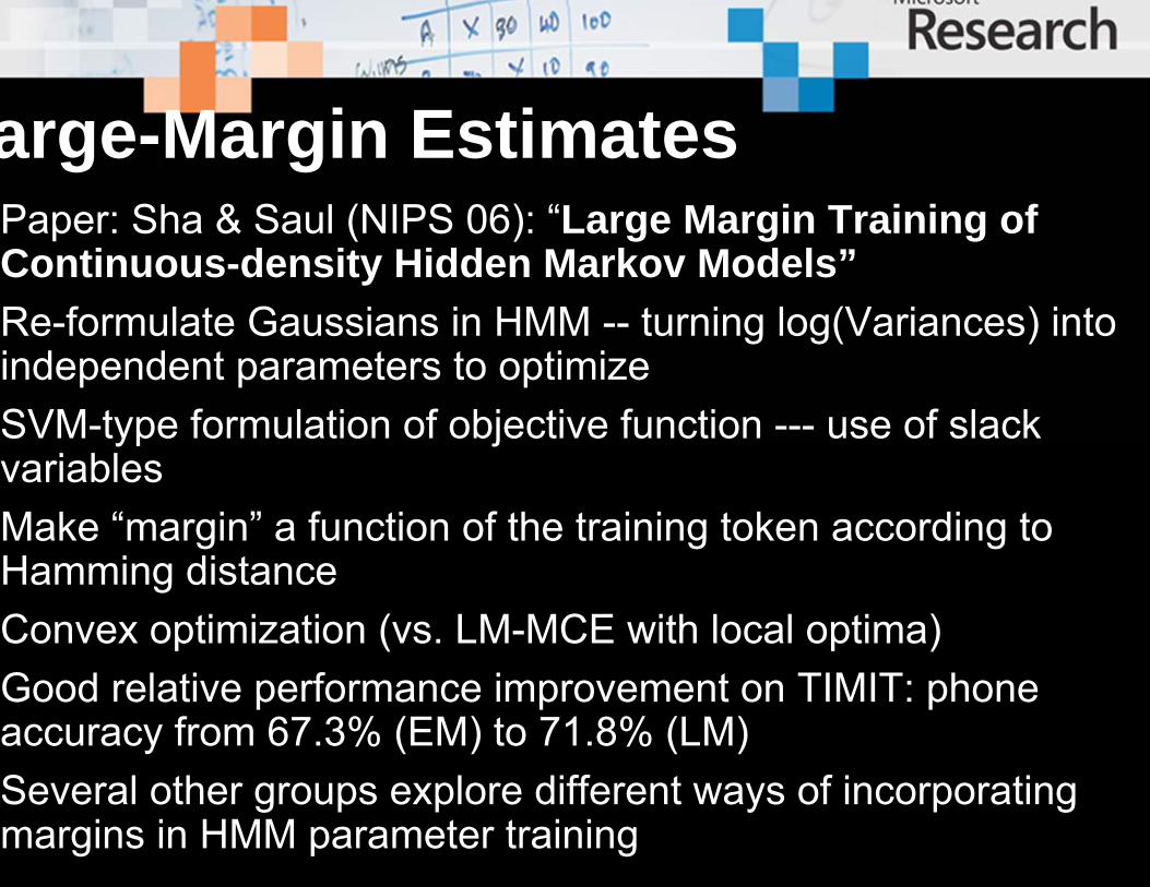
arge-Margin EstimatesPaper: Sha & Saul (NIPS 06): “Large Margin Training of Continuous-density Hidden Markov Models”Re-formulate Gaussians in HMM -- turning log(Variances) into independent parameters to optimizeSVM-type formulation of objective function --- use of slack variablesMake “margin” a function of the training token according to Hamming distanceConvex optimization (vs. LM-MCE with local optima)Good relative performance improvement on TIMIT: phone accuracy from 67.3% (EM) to 71.8% (LM)Several other groups explore different ways of incorporating margins in HMM parameter training

33
MCE in more detailMCE in more detail
OH EIGHT THREE correct label: Sr
OH EIGHT SIX competitor: sr,1
Observation. seq.: Xr x1, x2, x3, x4 ,…, xt ,…, xT
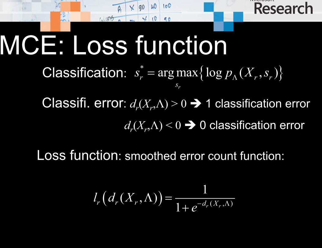
, ,1 ,( , ) log ( ) log ( )r r r r r rd X p X s p X SΛ ΛΛ = −Define misclassification measure:
sr,1: the top one incorrect (not equal to Sr) competing string
the case of using correct and top one incorrect competing tokens)
34
MCE: Loss functionMCE: Loss function
( ) ( , )
1( , )1 r rr r r d Xl d X
e− ΛΛ =+
Loss function: smoothed error count function:
Classification: { }* arg max log ( , )r
r r rs
s p X sΛ=
Classifi. error: dr(Xr,Λ) > 0 1 classification error
dr(Xr,Λ) < 0 0 classification error
35
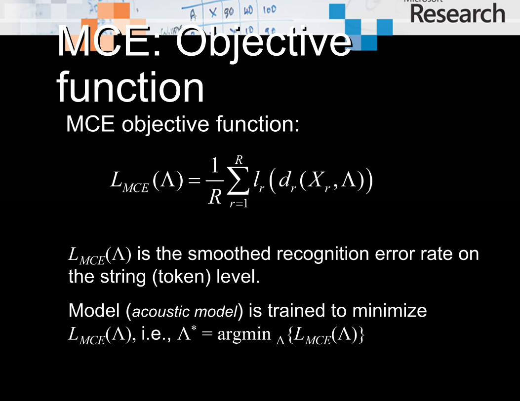
MCE: Objective MCE: Objective function function MCE objective function:
( )1
1( ) ( , )R
MCE r r rr
L l d XR =
Λ = Λ∑
LMCE(Λ) is the smoothed recognition error rate on the string (token) level.
Model (acoustic model) is trained to minimizeLMCE(Λ), i.e., Λ* = argmin Λ{LMCE(Λ)}
36
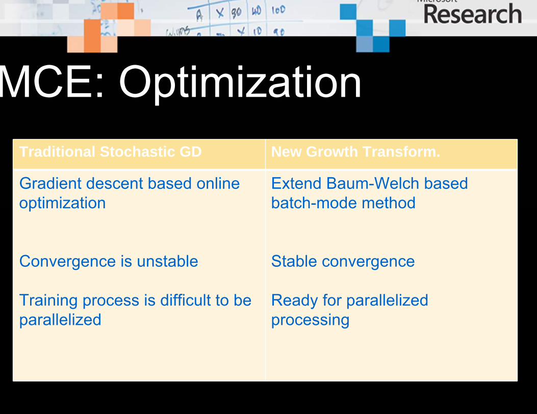
MCE: OptimizationMCE: OptimizationTraditional Stochastic GD New Growth Transform.
Gradient descent based online optimization
Convergence is unstable
Training process is difficult to be parallelized
Extend Baum-Welch based batch-mode method
Stable convergence
Ready for parallelized processing

Introduction to EBW or GT (Part Introduction to EBW or GT (Part I) I) Applied to rational function as the objective fcnt:
Equivalent auxiliary objective fctn (often easier toptimize):
where D is a Λ-independent constant. (see proof in SPM paper)
( )( )( )
GPH
ΛΛ =
Λ
( ; ) ( ) ( ) ( )F G P H D′ ′Λ Λ = Λ − Λ Λ +

Introduction to EBW or GT (Part Introduction to EBW or GT (Part II) II) Applied to the objective fcnt of the form:
Equivalent auxiliary objective fctn (easier to optimize):
(see proof in SPM paper & tech report)

39
MCE: OptimizationMCE: Optimization
MinimizingLMCE(Λ) =
∑ l ﴾d(·)﴿
MaximizingP(Λ) =
G(Λ)/H(Λ)
MaximizingF(Λ;Λ′) =
G-P′×H+D
MaximizingF(Λ;Λ′) =∑ f (·)
MaximizingU(Λ;Λ′) =∑ f ′(·)log f(·)
GT formula∂U(·)/∂Λ = 0
Λ =T(Λ′)
If Λ=T(Λ') ensures P(Λ)>P(Λ'), i.e., P(Λ) grows, then T(·) is called a growth transformation of Λ for P(Λ).
o Growth Transformation based MCE:
““Rational FunctionRational Function”” Form for Form for MEC Objective FunctionMEC Objective Function
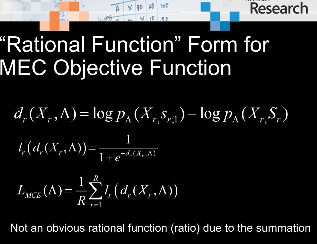
, ,1 ,( , ) log ( ) log ( )r r r r r rd X p X s p X SΛ ΛΛ = −
( ) ( , )
1( , )1 r rr r r d Xl d X
e− ΛΛ =+
( )1
1( ) ( , )R
MCE r r rr
L l d XR =
Λ = Λ∑
Not an obvious rational function (ratio) due to the summation
41
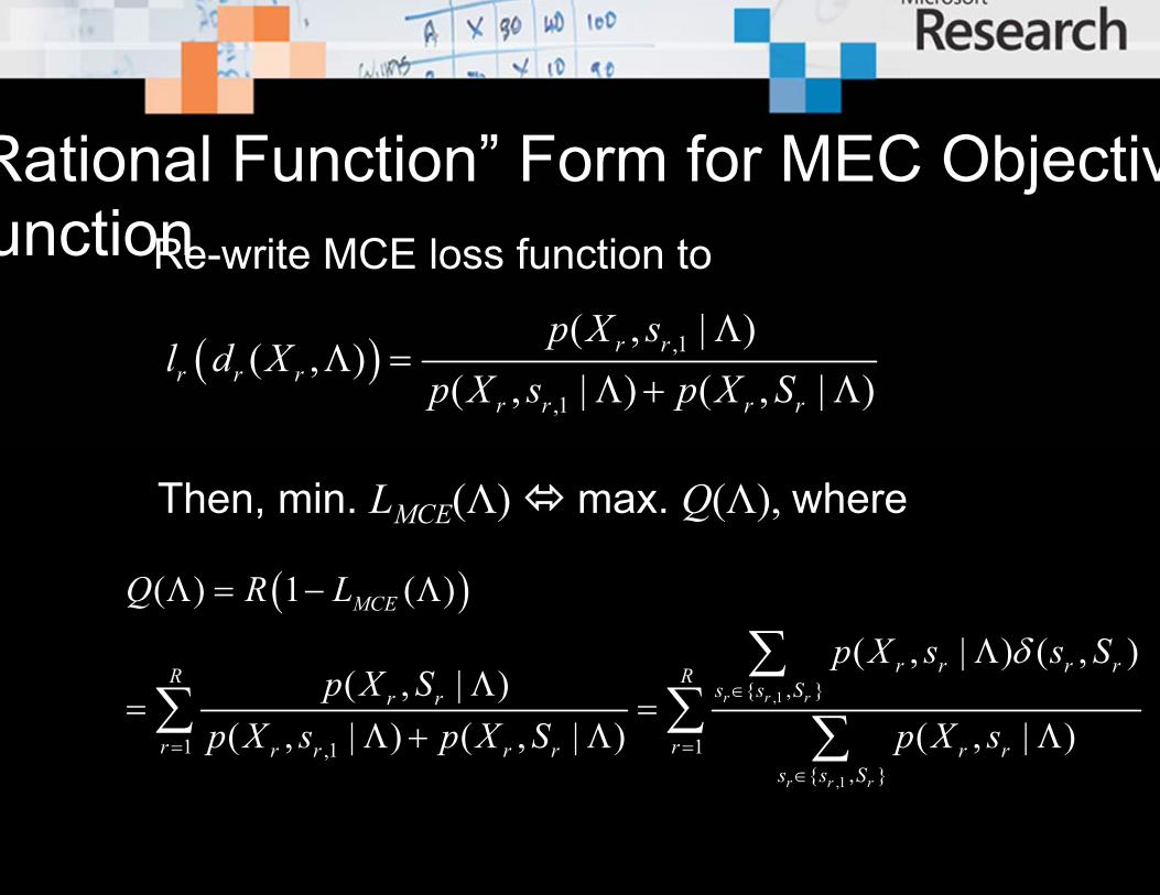
Rational FunctionRational Function”” Form for MEC ObjectivForm for MEC ObjectivunctionunctionRe-write MCE loss function to
Then, min. LMCE(Λ) max. Q(Λ), where
( ) ,1
,1
( , | )( , )
( , | ) ( , | )r r
r r rr r r r
p X sl d X
p X s p X SΛ
Λ =Λ + Λ
( )
,1
,1
{ , }
1 1,1{ , }
( ) 1 ( )
( , | ) ( , )( , | )
( , | ) ( , | ) ( , | )r r r
r r r
MCE
r r r rR Rs s Sr r
r rr r r r r rs s S
Q R L
p X s s Sp X S
p X s p X S p X s
δ∈
= =∈
Λ = − Λ
ΛΛ
= =Λ + Λ Λ
∑∑ ∑ ∑


Unified Objective FunctionUnified Objective FunctionCan do the same trick for MPE/MWEMMI objective function is naturally a rational function (due to logarithm in the MMI definition)Unified form:


45
MCE: Optimization (contMCE: Optimization (cont’’d)d)
( )( )( )
GPH
ΛΛ =
Λ
Coming back to MCE: its objective function can be re-formulated as a single fractional function P(Λ)
1
1
1 11
1 1
( ) ( ,..., , ,..., ) ( , )
( ) ( ,..., , ,..., )R
R
R
R R r rs s r
R Rs s
G p X X s s s S
H p X X s s
δΛ=
Λ
⎡ ⎤Λ = ⎢ ⎥⎣ ⎦Λ =
∑ ∑ ∑
∑ ∑
…
…
where

46
MCE: Optimization (contMCE: Optimization (cont’’d)d)Increasing P(Λ) can be achieved by maximizing
( ; ) ( ) ( ) ( )F G P H D′ ′Λ Λ = Λ − Λ Λ +
[ ]1( )( ) ( ) ( ; ) ( ; )HP P F FΛ
′ ′ ′ ′Λ − Λ = Λ Λ − Λ Λi.e.,
as long as D is a Λ-independent constant.
( ; ) ( , , | )[ ( ) ( )]q s
F p X q s C s P D′ ′Λ Λ = Λ − Λ +∑∑
Substitute G() and H() into F(),
(Λ′ is the parameter set obtained from last iteration)

47
[ ]( , , , ; ) ( ) ( ) ( , | , )f q s d s p q sχ χ′ ′Λ Λ = Γ Λ + Λ
( ; ) ( , , , ; )s q
F f q s dχ
χ χ′ ′Λ Λ = Λ Λ∑∑∫Reformulate F(Λ;Λ') to
where
F(Λ;Λ') is ready for EM-style optimization after applying GT theory (Part II)
( ) ( , ) ( , )[ ( ) ( )]s
X p q s C s Pδ χ′ ′Γ Λ = − Λ∑
1( ) ( , )
R
r rr
C s s Sδ=
=∑
Note: Γ(Λ′) is a constant, and log p(χ, q | s, Λ) is easy to decompose

48
( ) ( , , , ; ) log ( , , , ; )s q
U f q s f q s dχ
χ χ χ′ ′ ′Λ = Λ Λ Λ Λ∑∑∫
Increasing F(Λ;Λ') can be achieved by maximizing
( ) 0 ( )U T∂ Λ ′= ⇒ Λ = Λ∂Λ
So the growth transformation of Λ for CDHMM is:
Use EBM/GT (Part II) for E step.
log f(χ,q,s,Λ;Λ') is decomposable w.r.t Λ, so M step is easy to compute.

49
MCE: HMM estimation MCE: HMM estimation formulasformulasFor Gaussian mixture CDHMM,
, ,
,
( )
( )
m r r t m mr t
mm r m
j t
t x D
t D
γ μμ
γ
′Δ +=
Δ +
∑∑∑∑
, , ,
,
( )( - )( - ) ( - )( - )
( )
T Tm r r t m r t m m m m m m m m
r tm
m r mr t
t x x D D
t D
γ μ μ μ μ μ μ
γ
′ ′ ′⎡ ⎤Δ + Σ +⎣ ⎦Σ =
Δ +
∑∑∑∑
( ),1, ,1 , , , ,( ) ( | , ) ( | , ) ( ) ( )r rm r r r r r m r S m r st p S X p s X t tγ γ γ′ ′Δ = Λ Λ −where
1 12 1( | , ) | | exp ( ) ( )2
Tp x x xμ μ μ− −⎧ ⎫Σ ∝ Σ − − Σ −⎨ ⎬⎩ ⎭
GT of mean and covariance of Gaussian m is

50
MCE: HMM estimation MCE: HMM estimation formulasformulasSetting of Dm
[
],1
, ,1
,1 , ,
( | , ) ( | , ) ( )
( | , ) ( )
r
r
R
m r r r r m r Sr t
r r m r st
D E p S X p S X t
p s X t
γ
γ=
′ ′= ⋅ Λ Λ
′+ Λ
∑ ∑
∑
Theoretically,
set Dm so that f(χ,q,s,Λ;Λ') > 0
Empirically,

MCE: WorkflowMCE: Workflow
51
Training utterances
Last iterationModel Λ′
Recognition
GT-MCETraining transcripts
Competingstrings
New model Λnext iteration

52
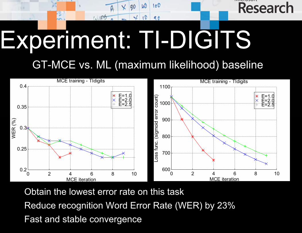
Experiment: TIExperiment: TI--DIGITSDIGITSVocabulary: “1” to “9”, plus “oh” and “zero”
Training set: 8623 utterances / 28329 words
Test set: 8700 utterances / 28583 words
33-dimentional spectrum feature: energy +10 MFCCs, plus ∆ and ∆∆ features.
Model: Continuous Density HMMs
Total number of Gaussian components: 3284
53
Experiment: TIExperiment: TI--DIGITSDIGITS
Obtain the lowest error rate on this taskReduce recognition Word Error Rate (WER) by 23%Fast and stable convergence
GT-MCE vs. ML (maximum likelihood) baseline
E=1.0E=2.0E=2.5
0 2 4 6 8 10600
700
800
900
1000
1100
MCE iteration
Loss
func
. (si
gmoi
d er
ror c
ount
)
MCE training - TIdigits
E=1.0E=2.0E=2.5
0 2 4 6 8 100.2
0.25
0.3
0.35
0.4
MCE iteration
WER
(%)
MCE training - TIdigits
HMM is an underlying model for modern speech recognizersFundamental properties of HMMStrengths and weaknesses of HMM for speech modeling and recognitionDiscriminative training for HMM as the “generative” model Reasonably good theory and practice for HMM discriminative training
Recommended