High-Sensitivity PET using
Optimised Continuous Cylindrical
Shell Nanocomposite and
Transparent Ceramic Scintillators
Keenan Wilson
School of Electrical and Data Engineering
University of Technology Sydney
A thesis presented for the degree of
Doctor of Philosophy
November 25, 2020

Certificate of Authorship /
Originality
I, Keenan Wilson declare that this thesis, is submitted in fulfilment of the require-
ments for the award of Doctor of Philosophy, in the School of Electrical and Data
Engineering at the University of Technology Sydney.
This thesis is wholly my own work unless otherwise referenced or acknowledged. In
addition, I certify that all information sources and literature used are indicated in
the thesis. This document has not been submitted for qualifications at any other
academic institution.
This research is supported by the Australian Government Research Training Pro-
gram.
© Copyright 2020 Keenan Wilson
i

Abstract
Positron emission tomography (PET) systems typically employ 2D or 3D arrays
of discrete monocrystalline rectangular prismatic scintillators, arranged in a ring
around the imaging object. As PET systems have evolved towards higher spatial
resolution and sensitivity, the number of crystals has increased while the dimen-
sions of the crystals have decreased, leading to ever-increasing costs and complexity
- particularly in total-body PET. At the same time, the need for optical isolation
between crystals limits packing efficiency and hence achievable sensitivity. The chief
alternative to discrete-crystal PET - monolithic scintillators with external photode-
tector arrays - introduces its own challenges, since producing large, high quality
scintillator crystals is expensive and technically challenging.
Two new classes of scintillator have recently emerged as alternatives to monocrys-
talline scintillators for gamma detection - nanocomposites, which combine scintillat-
ing nanoparticles with an organic polymer binder - and transparent ceramics. Both
are cheaper and easier to manufacture than monocrystalline scintillators, and can
be more easily formed into complex shapes - however, they are also less transpar-
ent and, in the case of nanocomposites, less dense. Neither has previously been
employed in PET systems to any significant degree.
In this work, a new PET system design is proposed which exploits the properties
of these new scintillators. Instead of discrete crystals or flat monolithic slabs, the
scintillator is formed into a continuous cylindrical shell, tiled on the inner and outer
surfaces with silicon photomultiplier photodetectors. The design aims to achieve
high sensitivity and competitive spatial resolution compared to similar discrete-
crystal PET systems.
Five nanocomposite and four transparent ceramic scintillators are evaluated,
and an optimisation method developed to maximise the probability of locating in-
ii

teractions between 511 keV photons and the scintillator within a given tolerance.
A technique for localising the endpoints of the lines of response in a monolithic
cylindrical shell is developed and evaluated for the best materials of both types.
A coincidence detection method based on deconvolution and spatio-temporal par-
titioning of photon clusters is developed and evaluated. Finally, a simulated PET
scan of several point sources inside the optimised scanner is performed, and im-
ages reconstructed using analytic and iterative algorithms; spatial resolution and
sensitivity are evaluated.
The promising results obtained in this work establish the feasibility of the pro-
posed design and confirm that the design objectives can be achieved. The design
offers a markedly different design envelope to conventional PET, and suggests a new
pathway to lower-cost total-body PET.
iii

Dedication
For my wife, Yukti.
iv

Acknowledgments
First and foremost I wish to thank my supervisor, Dr. Daniel Franklin at The
University of Technology Sydney. It goes without saying that without your guidance
and drive this project would not have been possible. I truly appreciate the sheer
amount of time, effort and caffeine you have contributed. I want to also thank my
co-supervisor, A/Prof Mehran Abolhasan for keeping me on the right track over
the years. Special thank you to Dr. Mitra Safavi-Naeini at ANSTO for her many
insights and contributions to our work. Thank you to A/Prof Justin Lipman and
Dr. Negin Shariati for accommodating me in their lab; it was such a great place
to work and I really enjoyed my time there. I want to also show my gratitude to
UTS for not only their financial support, but for the structural support within the
university, which has carried me to this point. Thank you to Dr. Matt Gaston
and ARCLab; without these resources, this work would literally not have been
possible. I also greatly appreciated receiving financial support from ANSTO and
AINSE for conference funding. My time at UTS would not have been the same
without Roumani Alabd. Thank you, not only for your contribution to this work,
but also for your friendship. All the best for your own PhD!
On a personal note, I would like to thank my family (Wilsons and Srivastavas)
for their love, guidance and especially patience. I especially want to thank my wife,
Yukti for her love, never ending support and belief in me.
Keenan Wilson
Sydney, Australia, 2020.
v

Contents
1 Introduction 1
1.1 Research Objectives and Overview . . . . . . . . . . . . . . . . . . . 5
1.1.1 Additional Research Contributions . . . . . . . . . . . . . . . 9
2 Literature Review 10
2.1 Positron Imaging . . . . . . . . . . . . . . . . . . . . . . . . . . . . . 10
2.1.1 Types of Detected Events . . . . . . . . . . . . . . . . . . . . 12
2.1.2 Photon Interactions with Matter . . . . . . . . . . . . . . . . 14
2.2 PET Radiotracers . . . . . . . . . . . . . . . . . . . . . . . . . . . . . 15
2.2.1 Metabolism . . . . . . . . . . . . . . . . . . . . . . . . . . . . 16
2.2.2 Blood Flow and Regional Perfusion . . . . . . . . . . . . . . . 17
2.2.3 Tumour Proliferation . . . . . . . . . . . . . . . . . . . . . . . 18
2.2.4 Positron Energy . . . . . . . . . . . . . . . . . . . . . . . . . . 18
2.3 PET Detectors . . . . . . . . . . . . . . . . . . . . . . . . . . . . . . 19
2.3.1 Detector Properties . . . . . . . . . . . . . . . . . . . . . . . . 19
2.3.2 Semiconductor Detectors . . . . . . . . . . . . . . . . . . . . . 21
2.3.3 Scintillation Detectors . . . . . . . . . . . . . . . . . . . . . . 21
2.3.4 Photomultiplier Tube . . . . . . . . . . . . . . . . . . . . . . . 23
2.3.5 Avalanche Photodiode . . . . . . . . . . . . . . . . . . . . . . 25
2.3.6 Silicon Photomultiplier . . . . . . . . . . . . . . . . . . . . . . 27
2.3.7 Detector Designs . . . . . . . . . . . . . . . . . . . . . . . . . 28
2.3.8 Alternative Detector Configurations . . . . . . . . . . . . . . . 33
2.3.9 Time-of-Flight PET . . . . . . . . . . . . . . . . . . . . . . . 34
2.4 Scintillation Materials . . . . . . . . . . . . . . . . . . . . . . . . . . 35
2.4.1 Scintillator Properties . . . . . . . . . . . . . . . . . . . . . . 35
vi

2.4.2 Nanocomposite Scintillators . . . . . . . . . . . . . . . . . . . 39
2.4.3 Transparent Ceramic Scintillators . . . . . . . . . . . . . . . . 43
2.5 Image Reconstruction . . . . . . . . . . . . . . . . . . . . . . . . . . . 45
2.5.1 Data Storage . . . . . . . . . . . . . . . . . . . . . . . . . . . 45
2.5.2 Filtered Backprojection . . . . . . . . . . . . . . . . . . . . . . 47
2.5.3 Backproject Then Filter . . . . . . . . . . . . . . . . . . . . . 49
2.5.4 Types of Filters . . . . . . . . . . . . . . . . . . . . . . . . . . 49
2.5.5 3D Image Reconstruction . . . . . . . . . . . . . . . . . . . . 51
2.5.6 Iterative Image Reconstruction . . . . . . . . . . . . . . . . . 53
2.5.7 The System Matrix . . . . . . . . . . . . . . . . . . . . . . . . 54
2.5.8 Iterative Algorithms . . . . . . . . . . . . . . . . . . . . . . . 56
2.5.9 Image Reconstruction Software . . . . . . . . . . . . . . . . . 58
2.6 Conclusion . . . . . . . . . . . . . . . . . . . . . . . . . . . . . . . . . 59
3 Monolithic Nanocomposite and Transparent Ceramic Scintillation
Detectors for use in Positron Emission Tomography 60
3.1 Introduction . . . . . . . . . . . . . . . . . . . . . . . . . . . . . . . . 60
3.2 Materials and Methods . . . . . . . . . . . . . . . . . . . . . . . . . . 63
3.2.1 Performance Metric and Optimisation Algorithm . . . . . . . 63
3.2.2 Simulation Parameters . . . . . . . . . . . . . . . . . . . . . . 65
3.2.3 Detector Geometry . . . . . . . . . . . . . . . . . . . . . . . . 65
3.2.4 GATE Parameters . . . . . . . . . . . . . . . . . . . . . . . . 66
3.2.5 Nanocomposite Loading . . . . . . . . . . . . . . . . . . . . . 67
3.2.6 Scintillation Event Position Determination . . . . . . . . . . . 68
3.2.7 Materials . . . . . . . . . . . . . . . . . . . . . . . . . . . . . 73
3.3 Results and Discussion . . . . . . . . . . . . . . . . . . . . . . . . . . 74
3.3.1 Calculation of the Optimal Scintillator Thickness . . . . . . . 74
3.3.2 Analysis of Photoelectric vs Compton Interactions . . . . . . . 75
3.3.3 Spatial error . . . . . . . . . . . . . . . . . . . . . . . . . . . . 82
3.4 Conclusion . . . . . . . . . . . . . . . . . . . . . . . . . . . . . . . . . 91
4 Localisation of the Lines of Response in a Continuous Cylindrical
Shell PET Scanner 93
vii

4.1 Introduction . . . . . . . . . . . . . . . . . . . . . . . . . . . . . . . . 93
4.2 Materials and methods . . . . . . . . . . . . . . . . . . . . . . . . . . 95
4.2.1 Materials . . . . . . . . . . . . . . . . . . . . . . . . . . . . . 95
4.2.2 Optimisation of scanner geometry . . . . . . . . . . . . . . . . 95
4.2.3 Localisation method . . . . . . . . . . . . . . . . . . . . . . . 98
4.2.4 Simulation . . . . . . . . . . . . . . . . . . . . . . . . . . . . . 100
4.3 Results . . . . . . . . . . . . . . . . . . . . . . . . . . . . . . . . . . . 100
4.3.1 GLuGAG:Ce . . . . . . . . . . . . . . . . . . . . . . . . . . . 101
4.3.2 LaF3:Ce-PS . . . . . . . . . . . . . . . . . . . . . . . . . . . . 105
4.3.3 Detector Sensitivity and Detection Accuracy . . . . . . . . . . 105
4.4 Discussion . . . . . . . . . . . . . . . . . . . . . . . . . . . . . . . . . 109
4.5 Conclusions and future work . . . . . . . . . . . . . . . . . . . . . . . 111
5 Efficient spatio-temporal deconvolution-based pulse pile-up correc-
tion for coincidence detection in monolithic-scintillator PET sys-
tems 112
5.1 Introduction . . . . . . . . . . . . . . . . . . . . . . . . . . . . . . . . 112
5.2 Materials and Methods . . . . . . . . . . . . . . . . . . . . . . . . . . 114
5.2.1 Coincidence Detection Technique . . . . . . . . . . . . . . . . 114
5.2.2 Impulse Response Generation . . . . . . . . . . . . . . . . . . 114
5.2.3 Single, 2-Coincidence and Multiple-Coincidence Detection . . 115
5.2.4 Line of Response Position Estimation . . . . . . . . . . . . . . 118
5.2.5 Geometry . . . . . . . . . . . . . . . . . . . . . . . . . . . . . 121
5.2.6 GATE Simulation Parameters . . . . . . . . . . . . . . . . . . 121
5.3 Results . . . . . . . . . . . . . . . . . . . . . . . . . . . . . . . . . . . 122
5.3.1 Algorithm Detection Efficiency . . . . . . . . . . . . . . . . . 122
5.3.2 Detection Efficiency by Interaction Type . . . . . . . . . . . . 123
5.4 Discussion . . . . . . . . . . . . . . . . . . . . . . . . . . . . . . . . . 123
5.5 Conclusion . . . . . . . . . . . . . . . . . . . . . . . . . . . . . . . . . 124
6 Design and Simulation of a Brain PET Scanner with a Continuous
Cylindrical Shell Monolithic Scintillator 125
6.1 Introduction . . . . . . . . . . . . . . . . . . . . . . . . . . . . . . . . 125
viii

6.2 Materials and Methods . . . . . . . . . . . . . . . . . . . . . . . . . . 127
6.2.1 Simulation Parameters . . . . . . . . . . . . . . . . . . . . . . 127
6.2.2 Image Reconstruction . . . . . . . . . . . . . . . . . . . . . . . 127
6.2.3 Image Correction . . . . . . . . . . . . . . . . . . . . . . . . . 129
6.3 Results . . . . . . . . . . . . . . . . . . . . . . . . . . . . . . . . . . . 134
6.3.1 Image Reconstruction . . . . . . . . . . . . . . . . . . . . . . . 134
6.3.2 Spatial Resolution Measurements . . . . . . . . . . . . . . . . 134
6.4 Discussion . . . . . . . . . . . . . . . . . . . . . . . . . . . . . . . . . 142
6.5 Conclusion . . . . . . . . . . . . . . . . . . . . . . . . . . . . . . . . . 145
7 Conclusion 146
7.1 Summary . . . . . . . . . . . . . . . . . . . . . . . . . . . . . . . . . 147
7.2 Recommendations & Future Work . . . . . . . . . . . . . . . . . . . . 150
7.3 Concluding Remarks . . . . . . . . . . . . . . . . . . . . . . . . . . . 152
A Code Documentation 173
A.1 Nanocomposite & Transparent Ceramic Optimal Thickness Code . . . 173
A.1.1 Code Availability . . . . . . . . . . . . . . . . . . . . . . . . . 173
A.1.2 Software Requirements . . . . . . . . . . . . . . . . . . . . . . 173
A.1.3 GATE Code - How to Run . . . . . . . . . . . . . . . . . . . . 173
A.1.4 MATLAB Code - How to Run . . . . . . . . . . . . . . . . . . 175
A.2 Continuous Cylindrical Shell PET Code . . . . . . . . . . . . . . . . 176
A.2.1 Code Availability . . . . . . . . . . . . . . . . . . . . . . . . . 176
A.2.2 Software Requirements . . . . . . . . . . . . . . . . . . . . . . 176
A.2.3 GATE Code - How to Run . . . . . . . . . . . . . . . . . . . . 177
A.2.4 MATLAB Code - How to Run . . . . . . . . . . . . . . . . . . 179
A.2.5 STIR Code - How to Run . . . . . . . . . . . . . . . . . . . . 185
ix

List of Figures
2.1 Positron annihilation. . . . . . . . . . . . . . . . . . . . . . . . . . . . 11
2.2 Types of detected events: true, random, scatter and multiple. . . . . 13
2.3 Compton angular probability distribution. . . . . . . . . . . . . . . . 15
2.4 Scintillation energy states. . . . . . . . . . . . . . . . . . . . . . . . . 23
2.5 Operation of a photomultiplier tube (PMT). . . . . . . . . . . . . . . 24
2.6 Operation of a avalanche photodiode (APD) . . . . . . . . . . . . . . 26
2.7 Scintillation detector designs featuring depth encoding. . . . . . . . . 31
2.8 Time-of-flight PET . . . . . . . . . . . . . . . . . . . . . . . . . . . . 35
2.9 Scintillator pulse shape. . . . . . . . . . . . . . . . . . . . . . . . . . 37
2.10 Calculated optical and gamma photon attenuation lengths in nanocom-
posite materials. . . . . . . . . . . . . . . . . . . . . . . . . . . . . . . 42
2.11 Construction of a sinogram from projection data. . . . . . . . . . . . 46
2.12 Filter functions used for 2D Filtered Back-Projection. . . . . . . . . . 50
2.13 Iterative image reconstruction: the system matrix. . . . . . . . . . . . 55
2.14 Iterative reconstruction algorithm flow diagram. . . . . . . . . . . . . 57
3.1 Simulated photoelectric interaction captured in GATE. . . . . . . . . 66
3.2 Nanocomposite scintillator loading factor determination. . . . . . . . 69
3.3 Position of interaction estimation: scintillation photon maps. . . . . . 70
3.3 Position of interaction estimation (continued): analytic model fitting. 71
3.4 Geometry of the photon distribution parametric model. . . . . . . . . 72
3.5 Percentage of events detected as a function of scintillator thicknesses:
nanocomposite materials - Gd2O3 PVT & LaBr3:Ce PS. . . . . . . . 76
3.5 Percentage of events detected as a function of scintillator thicknesses
(continued): nanocomposite materials - LaF3:Ce OA & LaF3:Ce PS. . 77
x

3.5 Percentage of events detected as a function of scintillator thicknesses
(continued): nanocomposite materials - YAG:Ce PS. . . . . . . . . . 78
3.6 Percentage of events detected as a function of scintillator thicknesses:
transparent ceramic materials - GAGG:Ce & GLuGAG:Ce . . . . . . 79
3.6 Percentage of events detected as a function of scintillator thicknesses
(continued): transparent ceramic materials - GYGAG:Ce & LuAG:Pr 80
3.7 Estimated position of interaction error (∆X & ∆Y) as a function of
scintillator depth (LaF3:Ce-PS) . . . . . . . . . . . . . . . . . . . . . 86
3.7 Estimated position of interaction error (∆Z & total error) as a func-
tion of scintillator depth (LaF3:Ce-PS)(continued) . . . . . . . . . . . 87
3.8 Estimated position of interaction error (∆X & ∆Y) as a function of
scintillator depth (GLuGAG:Ce) . . . . . . . . . . . . . . . . . . . . . 88
3.8 Estimated position of interaction error (∆Z & total error) as a func-
tion of scintillator depth (GLuGAG:Ce)(continued) . . . . . . . . . . 89
4.1 Geometry of the simulated cylindrical shell scanner . . . . . . . . . . 97
4.2 GLuGAG:Ce: endpoint errors (R and Z) vs depth of penetration. . . 102
4.2 GLuGAG:Ce: endpoint errors (θ and total error) vs depth of pene-
tration. . . . . . . . . . . . . . . . . . . . . . . . . . . . . . . . . . . . 103
4.2 GLuGAG:Ce: LOR error vs depth of interaction. . . . . . . . . . . . 104
4.3 LaF3:Ce-PS: endpoint errors (R and Z) vs depth of penetration. . . . 106
4.3 LaF3:Ce-PS: endpoint errors (θ and total error) vs depth of penetration.107
4.3 GLuGAG:Ce: LOR error vs depth of interaction. . . . . . . . . . . . 108
5.1 Generated impulse responses for five discrete radial bins. . . . . . . . 116
5.2 Coincidence detection: spatial event sorting . . . . . . . . . . . . . . 118
5.3 Coincidence detection by pulse deconvolution. . . . . . . . . . . . . . 119
5.4 Line of response generation . . . . . . . . . . . . . . . . . . . . . . . 120
6.1 Random, normalisation and attenuation corrections in projection and
image space. . . . . . . . . . . . . . . . . . . . . . . . . . . . . . . . . 132
6.2 2D analytic image reconstruction of three 3 MBq 18F sources encap-
sulated in cylindrical water phantoms, using STIR’s FBP2D algorithm.135
xi

6.3 3D analytic image reconstruction of three 3 MBq 18F sources en-
capsulated in cylindrical water phantoms, using STIR’s FBP3DRP
algorithm. . . . . . . . . . . . . . . . . . . . . . . . . . . . . . . . . . 136
6.4 3D iterative image reconstruction of three 3 MBq 18F sources en-
capsulated in cylindrical water phantoms, using STIR’s OSMAPOSL
algorithm. . . . . . . . . . . . . . . . . . . . . . . . . . . . . . . . . . 137
6.5 Intensity profile of the FBP2D-reconstructed image along the X axis. 138
6.6 Intensity profile of the FBP2D-reconstructed image along the Y and
Z axes. . . . . . . . . . . . . . . . . . . . . . . . . . . . . . . . . . . . 139
6.7 Intensity profile of the FBP3DRP-reconstructed image along the X
axis. . . . . . . . . . . . . . . . . . . . . . . . . . . . . . . . . . . . . 140
6.8 Intensity profile of the FBP3DRP-reconstructed image along the Y
and Z axes. . . . . . . . . . . . . . . . . . . . . . . . . . . . . . . . . 141
6.9 Intensity profile of the OSEM-reconstructed image along the X axis. . 142
6.10 Intensity profile of the OSEM-reconstructed image along the Y and
Z axes. . . . . . . . . . . . . . . . . . . . . . . . . . . . . . . . . . . . 143
xii

List of Tables
2.1 PET radioisotopes. . . . . . . . . . . . . . . . . . . . . . . . . . . . . 16
2.2 A comparison of typical photodetector properties. . . . . . . . . . . . 29
2.3 Single crystal scintillation materials. . . . . . . . . . . . . . . . . . . . 36
2.4 Physical and optical properties of nanocomposite scintillators. . . . . 40
2.5 Physical and optical properties of transparent ceramic scintillators. . 44
3.1 Summary of nanocomposite loading factors (by % volume) used in
GATE simulations. . . . . . . . . . . . . . . . . . . . . . . . . . . . . 69
3.2 Summary of optimal scintillator thickness and detection probability
for nanocomposite and transparent ceramic materials. . . . . . . . . . 78
3.3 Distribution of photoelectric and Compton-scattered interactions for
a 1 cm thick scintillator slab. . . . . . . . . . . . . . . . . . . . . . . 83
3.4 Distribution of photoelectric and Compton-scattered interactions for
a 2 cm thick scintillator slab. . . . . . . . . . . . . . . . . . . . . . . 83
3.5 Distribution of photoelectric and Compton-scattered interactions for
a scintillator slab equal to the HVL. . . . . . . . . . . . . . . . . . . . 84
3.6 Distribution of photoelectric and Compton-scattered interactions for
a scintillator slab equal to the optimal thickness. . . . . . . . . . . . . 84
3.7 Mean and median errors in the estimation of the point of interaction
within scintillators of 1 cm thickness. . . . . . . . . . . . . . . . . . . 85
3.8 Mean and median errors in the estimation of the point of interaction
within scintillators of 2 cm thickness. . . . . . . . . . . . . . . . . . . 90
3.9 Mean and median errors in the estimation of the point of interaction
within scintillators of thickness equal to the HVL. . . . . . . . . . . . 90
xiii

3.10 Mean and median errors in the estimation of the point of interaction
within scintillators with thickness equal to the optimum. . . . . . . . 91
4.1 Properties of scintillator materials used in the cylindrical shell PET
scanner. . . . . . . . . . . . . . . . . . . . . . . . . . . . . . . . . . . 95
4.2 Scanner dimensions and expected detection efficiency . . . . . . . . . 96
4.3 GLuGAG:Ce error statistics summary . . . . . . . . . . . . . . . . . . 101
4.4 LaF3:Ce-PS error statistics summary . . . . . . . . . . . . . . . . . . 105
4.5 Fractions of decays yielding usable LORs and accuracy of detected
endpoints. . . . . . . . . . . . . . . . . . . . . . . . . . . . . . . . . . 109
5.1 True, random and missed detections as a percentage of the total num-
ber of decays. . . . . . . . . . . . . . . . . . . . . . . . . . . . . . . . 122
5.2 Detection type and probability of occurrence. . . . . . . . . . . . . . 123
6.1 STIR parameters. . . . . . . . . . . . . . . . . . . . . . . . . . . . . . 130
6.2 Full width at half maximum (FWHM) of the intensity profiles at zero
degrees in the transverse plane (x-axis of the system). . . . . . . . . . 138
6.3 Full width at half maximum (FWHM) of the intensity profiles at 90
degrees in the transverse plane (y-axis of the system). . . . . . . . . . 140
6.4 Full width at half maximum (FWHM) of the intensity profiles at 90
degrees in the coronal plane (z-axis of the system). . . . . . . . . . . 140
xiv
Chapter 1
Introduction
Positron emission tomography (PET) is a widely-used nuclear medical imaging
modality with broad clinical, biological and human health research applications.
In contrast to imaging techniques such as 2D X-ray imaging, X-ray computed to-
mography (CT), some variants of magnetic resonance imaging (Structural MRI and
Diffusion-based MRI), which produce a structural map of the imaging object, PET
is a functional imaging modality, which elucidates biological processes (as opposed
to structures in close to real time). PET is commonly used for cancer diagnosis and
treatment planning, where it delineates regions of tissue with elevated metabolism
(indicating rapid and abnormal cellular growth). It is also a critical tool in biological
research, since by choosing an appropriate radiotracer, a wide variety of different
biological processes can be quantitatively evaluated in living animals.
PET images are either acquired over a period of up to around 30 minutes to
obtain a single static three dimensional image, or acquired in temporal frames with
durations of seconds to minutes to create 4-dimensional spatio-temporal images,
which map the uptake, distribution and excretion of positron-emitting radiotracers
inside the body. Examples of PET applications include measurement of blood flow,
respiration, metabolism, and receptor density and activation in the brain. This
wealth of information is invaluable both for clinical diagnosis and the development
of treatment plans for cancer, and also in the research sphere for studies involving
small and large animals - especially the preclinical evaluation of new drugs.
During PET imaging, a compound known as a radiotracer, which includes a
short-lived positron-emitting radioisotope such as 18F, 15O or 11C, is injected into
1

the patient. The choice of compound depends on the target of interest - for example,
when PET is used for cancer imaging, the most common radiotracer is an analogue
of glucose, 18F-fluorodeoxyglucose (FDG), which functions almost identically to nor-
mal glucose in the body. During the scan, the radiotracer circulates through the
bloodstream, and some fraction interacts biochemically with the target tissue (in
FDG for example, via an intracellular metabolic trapping process). The resulting
physical concentration distribution of the radiotracer therefore corresponds to the
extent to which it is trapped within the target cells. PET is an exceptionally sen-
sitive imaging modality. While other modalities can provide functional information
in a living subject, no imaging technique can approach the sensitivity of PET for
molecular imaging; it is able to determine concentrations of radiopharmaceuticals
at the nmol or even pmol range, allowing for non-invasive imaging, monitoring of
disease and elucidation of biological pathways.
The radioisotope undergoes β+ decay (concentrated at, but not exclusive to the
target cells), and the emitted positron travels a short distance before annihilating
with an electron to convert 100% of their combined rest mass into a pair of 511 keV
gamma photons, radiating away from the point of annihilation in almost exactly
opposite directions (the slight acollinearity is due to the non-zero pre-annihilation
momentum of the positron and electron). The emitted antiparallel gamma photons
simultaneously travel away from the point of annihilation, and due to their high
energy, the majority will exit the body without scattering. These photons may be
detected by an external photon detector array.
Due to the near-antiparallel direction of emission of the annihilation photons,
the detection of two near-simultaneous 511 keV photons enables a line of response
(LOR) to be drawn between the points of detection. The fundamental assumption
in PET is that for most of these coincidences, a decay has occurred somewhere
along this line (or close to it), since the positron only travels a short distance from
the point of radionuclide decay before annihilating (less than 1 mm on average in
the case of 18F). By accumulating many of these LORs over time in a sinogram
(a 3D or 4D histogram of the orientation and position of the LORs in cylindrical
coordinates of (R, θ, φ(t)), where θ and φ are the transaxial azimuth and elevation
of the LOR and R is the minimum distance of the LOR from the z-axis), a unique
2

mathematical representation of the radiotracer distribution can be constructed. A
number of different algorithms, such as filtered backprojection (FBP) or maximum
likelihood expectation maximisation (MLEM) may then be used to transform this
sinogram from projection space into an image domain representation of spatial (or
spatio-temporal) distribution of the radiotracer. Several additional corrective steps
are then applied to compensate for attenuation, scatter, random (false positive)
coincidences and the non-uniform sensitivity of the detector geometry to different
potential lines of response (normalisation).
The number of gamma photons available for potential detection is limited by
the maximum radiotracer dose which can safely be administered to the patient,
and the half-life of the radiotracer. It is therefore very import to have a highly
sensitive detector system that is capable of detecting as many of these photons as
possible, since this is directly related to the quality of the resulting image (in par-
ticular, it determines the achievable signal to noise ratio). The high energy of these
photons makes detection challenging; direct detection sensitivity in semiconductor
detectors (e.g. reverse-biased silicon diode detectors) is extremely low due to the
low density and low effective atomic number (Zeff ) of common semiconductor ma-
terials and the limited thickness of such detectors (around 1 mm is the maximum
feasible thickness which can be achieved). Instead, the normal approach in PET
is to use a scintillator, most commonly a high density inorganic crystal with small
amounts of certain rare-earth dopants, to absorb some or all of the energy of the
gamma photon (depending on the mode of interaction) and re-emit the energy as
a shower of lower-energy optical photons [1]. These photons can be detected and
counted easily using semiconductor photodetectors, and the total energy deposited
by the gamma photon interaction estimated from the number of detected optical
photons. Generating accurate lines of response with full angular coverage requires
that the positron-emitting object be surrounded by a ring (or multiple parallel rings)
of scintillation detectors.
Improving the performance of PET systems for clinical and biological research
applications is a major research problem, driven largely by the need for higher qual-
ity images, and improved cost-effectiveness. Most current PET systems have an
absolute sensitivity for coincidence detection of the order of a few percent only [2,
3
3], which limits the achievable signal-to-noise ratio of the system. More recently,
there has been growing interest in total-body PET, in which the axial field of view
extends to encompass the entire body simultaneously (as opposed to whole-body
PET, in which the patient’s whole body is progressively scanned via successive axial
translations through a short ring of detectors) [3, 4]. While this substantially im-
proves sensitivity by virtue of the improved solid angle coverage around the imaging
object, it comes at an enormous cost due to the huge number of tiny scintillation
crystals and photodetectors required. However, at present, this is the most popular
strategy for increased detection sensitivity in PET.
Silicon photomultipliers (SiPMs) have become a more viable option in PET re-
cently, due to improving responsiveness and probability of detection; adding an
alternate solution to the sensitivity problem - improving timing resolution (when
coupled with fast, high density and bright Lutetium based scintillators). Time-of-
flight PET, as it is known, can improve effective system sensitivity gain by mea-
suring the temporal difference between detections of the two annihilation photons.
The position of the original annihilation event may then be localised to within a
certain range along the LOR and the noise reduced along those particular voxels
(i.e. boosting SNR).
Spatial resolution in PET is limited by a number of factors, including the size
of the scintillator crystals, photon acollinearity and positron range (although the
latter can be largely corrected using image deconvolution methods). Shrinking the
scintillator crystals only works up to a point, beyond which efficient coupling of
the individual crystals to photodetectors becomes impractical due to the interstitial
reflective coatings needed. Scintillation detectors are also inherently expensive and
difficult to manufacture, as a result scintillator crystal itself accounts for a large
proportion of the overall cost of the scanner [5, 6, 4]. An alternative approach
is to use monolithic scintillator slabs coupled to photodetector arrays to analyti-
cally estimate the location of the point of interaction within the slab. Monolithic
slabs have a higher spatial coverage compared to regular block scintillation detec-
tors and are capable of measuring the depth of interaction (which in turn improves
timing resolution [7, 8]). However, the production of large crystals of uniform qual-
ity from high-performance scintillator materials is challenging and very expensive.
4
Furthermore, accurate localisation is challenging when the interaction occurs near
the boundary of the rectangular slabs, and algorithms capable of handling this well
(typically based on neural networks) are computationally expensive.
New approaches which seek to simultaneously address the problems of achiev-
ing high spatial resolution and high sensitivity without greatly inflating the cost
of a scanner would clearly be of enormous value in the field of PET, and would
expand the availability and utility of this important imaging modality both for
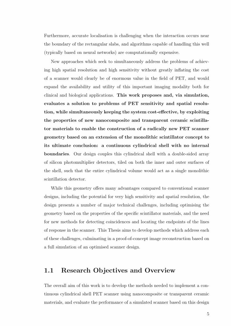
clinical and biological applications. This work proposes and, via simulation,
evaluates a solution to problems of PET sensitivity and spatial resolu-
tion, while simultaneously keeping the system cost-effective, by exploiting
the properties of new nanocomposite and transparent ceramic scintilla-
tor materials to enable the construction of a radically new PET scanner
geometry based on an extension of the monolithic scintillator concept to
its ultimate conclusion: a continuous cylindrical shell with no internal
boundaries. Our design couples this cylindrical shell with a double-sided array
of silicon photomultiplier detectors, tiled on both the inner and outer surfaces of
the shell, such that the entire cylindrical volume would act as a single monolithic
scintillation detector.
While this geometry offers many advantages compared to conventional scanner
designs, including the potential for very high sensitivity and spatial resolution, the
design presents a number of major technical challenges, including optimising the
geometry based on the properties of the specific scintillator materials, and the need
for new methods for detecting coincidences and locating the endpoints of the lines
of response in the scanner. This Thesis aims to develop methods which address each
of these challenges, culminating in a proof-of-concept image reconstruction based on
a full simulation of an optimised scanner design.
1.1 Research Objectives and Overview
The overall aim of this work is to develop the methods needed to implement a con-
tinuous cylindrical shell PET scanner using nanocomposite or transparent ceramic
materials, and evaluate the performance of a simulated scanner based on this design
5

concept, including the development of a complete pipeline for transforming list-mode
data to a corrected 3D image.
The specific research objectives of this Thesis are:
1. To develop methods for objectively comparing the performance of different
nanocomposite and transparent ceramic scintillator materials, including de-
velopment of accurate simulation models for different materials and the devel-
opment of appropriate performance metrics which are relevant to PET perfor-
mance, and evaluate this for a range of promising nanocomposite and trans-
parent ceramic scintillator materials;
2. To develop a technique for optimising the thickness of the cylindrical scin-
tillator shell to maximise the performance metric defined above for a given
scintillator, and find this optimised thickness for each of the evaluated scintil-
lator materials;
3. To adapt an existing approach for localising the point of interaction in a flat
monolithic scintillator to a continuous cylindrical shell;
4. To design a method for coincidence detection suitable for use in the proposed
scanner design; and
5. To implement a simulated scanner using one of the best-performing materials,
optimised according to the developed performance metric, simulate several
simple phantom and/or point source models and evaluate its sensitivity and
spatial resolution.
Each chapter of the Thesis will solve important engineering design questions,
contributing to the overall aim.
Chapter 2 provides a comprehensive review of literature which is relevant to
the overall aim. This includes a broad overview of current PET systems and the
physical interactions taking place within them. The photodetectors, scintillation
materials and system architecture are discussed in detail, including a review of the
root causes of system limitations and how they might be addressed. Finally, image
reconstruction theory is explored, including analytic and iterative algorithms, for
use in quantifying an output. The literature review is the first step in identifying
6

why the system limitations are present, what has already been done to address them
and how we might approach a new solution to the sensitivity and spatial resolution
problems.
Chapter 3 aims to make a determination of which nanocomposite or transparent
ceramic materials might be suitable for use in the proposed system. Since Rayleigh
scattering is a limiting factor for the optical transparency of the nanocomposites /
ceramics, it is also important to find the optimal thickness for the scintillator slab;
finding the maximum probability of gamma detection for a desired position estima-
tion accuracy. Each scintillator material has been simulated as a simple monolithic
block detector with dual-sided readout, using Monte Carlo-based methods over a
range of scintillator thicknesses, with an analytic algorithm used to determine the
point of interaction. Importantly, this chapter defines a critical performance metric
for monolithic scintillators based on the probability with which an interaction can
be localised to within a specified tolerance. This metric is then used to optimise
the scintillator thickness for each of the evaluated materials. A detailed statistical
analysis of the spatial error distributions and fraction of Compton and photoelec-
tric events is performed for each optimised scintillator, and the best-performing
nanocomposite and transparent ceramic materials are identified.
This chapter resulted in the following publications:
� Keenan J. Wilson, Roumani Alabd, Mehran Abolhasan, Mitra Safavi-Naeini,
and Daniel R. Franklin. Optimisation of monolithic nanocomposite and trans-
parent ceramic scintillation detectors for positron emission tomography. Sci
Rep 10, 1409 (2020).
� K. Wilson, IEEE, R. Alabd, IEEE, and D. R. Franklin. Optimisation of
Monolithic Nanocomposite and Ceramic Garnet Scintillator Thickness for PET.
Poster presentation at 2018 IEEE Nuclear Science Symposium and Medical
Imaging Conference (NSS/MIC), Sydney, Australia.
Possible geometries for the fully monolithic, continuous cylindrical shell PET
architecture are presented in Chapter 4. Two geometries are presented, using ma-
terials which were identified to be the most suitable from the previous chapter;
GLuGAG:Ce and LaF3:Ce-polystyrene, each with a shell thickness equivalent to the
7

optimal thickness for a median euclidean distance error of <5 mm. The main aim of
this chapter is to demonstrate that this geometry is potentially feasible for PET, and
successfully generating lines of response from coincident detections, which may then
be used in image reconstruction algorithms. A novel methodology for localisation
of gamma pairs and generation of a line of response is described and a statistical
analysis of the error in measurement of the LORs are presented, as well as an initial
measurement for sensitivity of the scanner. Sensitivity is presented as the fraction
of annihilation events which yield usable LORs.
This work resulted in the following publication:
� Wilson, K.J., Alabd, R., Abolhasan, M., Franklin, D.R. and Safavi-Naeini,
M., 2019, July. Localisation of the Lines of Response in a Continuous Cylindri-
cal Shell PET Scanner. In 2019 41st Annual International Conference of the
IEEE Engineering in Medicine and Biology Society (EMBC) (pp. 4844-4850).
IEEE.
Due to the radical differences between the proposed scanner architecture and
conventional pixellated scanners, existing methods for coincidence detection can-
not be applied. Chapter 5 presents a methodology for coincidence detection by
segmenting the scanner into sub-regions, accumulating events in each as a set of
time-domain signals, and deconvolving them by the scintillator impulse response to
correct for pulse pile-up, and then performing spatio-temporal cluster analysis to
identify probable coincidence events. The results are broken down into the fraction
of true coincidences detected and compared to the fraction of false positives and
false negatives for different types of interactions.
This work has resulted in the preparation of the following paper for submission
to Physics in Medicine and Biology:
� Wilson, K.J., Alabd., R, Safavi-Naeini, M., Franklin, D.R., Efficient spatio-
temporal deconvolution-based pulse pile-up correction for coincidence detec-
tion in monolithic-scintillator PET systems, To be submitted to Physics in
Medicine & Biology
Chapter 6 presents a reconstruction of an image of a number of simulated point
sources placed inside the field of view, using LORs generated by the scanner and
8

the methods described in the previous two Chapters. The aim is to firstly determine
whether or not the scanner can actually produce a reasonable image and secondly,
measure the spatial resolution of the point source image by measuring the full width
at half maximum of the line profile through each point source. Post-processing for
randoms correction and attenuation corrected normalisation of the image is also
demonstrated.
An extended version of the this chapter is currently in preparation as a paper
for submission to IEEE Transactions on Medical Imaging:
� Wilson, K.J., Alabd., R, Safavi-Naeini, M., Franklin, D.R., Characterisation
of a Simulated Continuous Cylindrical Shell PET Scanner with Nanocomposite
and Ceramic Scintillators, To be submitted to IEEE Transactions on Medical
Imaging.
Finally, Chapter 7 summarises the results and implications of this work, and
provides recommended directions for continuation of this work in the future.
1.1.1 Additional Research Contributions
A number of additional research publications and presentations are listed below:
� Alabd, R., Safavi-Naeini, M., Wilson, K.J., Rosenfeld, A.B. and Franklin,
D.R., 2018. A simulation study of BrachyShade, a shadow-based internal
source tracking system for HDR prostate brachytherapy. Physics in Medicine
& Biology, 63 (20), p.205019.
� R. Alabd, K. Wilson, D. R. Franklin. Source Tracking in a Scattering
Medium via Fast Hierarchical Pattern Matching. Oral presentation at 2018
IEEE Nuclear Science Symposium and Medical Imaging Conference (NSS/MIC),
Sydney, Australia.
� A. M. Ahmed, A. Chacon, K. Wilson, D. Franklin, K. Bambery, A. Rosenfeld,
S. Guatelli, M. Safavi-Naeini. Sparse time-of-flight in-beam PET for quality
assurance in particle therapy. Poster presentation at 2019 IEEE Nuclear Sci-
ence Symposium and Medical Imaging Conference (NSS/MIC), Manchester,
United Kingdom.
9

Chapter 2
Literature Review
2.1 Positron Imaging
Positron emission tomography (PET) is a well-established nuclear medical imaging
modality which is seeing clinical use in oncology, neurology and cardiology, as well
as a number of research applications such as the monitoring of disease therapies and
drug effectiveness. Imaging is based on the capture of radiation from an internal
energy source in the form of an injected radio-labelled tracer. When the radiotracer
is injected into the body, it undergoes decay, releasing positrons which combine
with nearby electrons in what is known as an annihilation event ; a complete mass
to energy conversion in accordance with Einstein’s famous equation, E = mc2,
producing two 511 keV gamma photons, travelling in opposing directions from the
point of interaction (See Figure 2.1).
A ring of high density, high effective atomic number scintillation detectors en-
compassing the field of view, are used in the detection of these high energy gamma
photons. An event is stored only if both gamma photons are detected within spe-
cific timing and energy windows; known as a coincidence detection. The original
annihilation event is known to lie somewhere along a line of response between the
two detectors where the scintillation interactions occurred and these stored lines of
response are subsequently used in the reconstruction of the original image, using
either analytic or iterative reconstruction algorithms.
The predetermined time frame is known as a coincidence window and exists
because there will always be some variation in the detection time of the two photons.
10

Field of view
β+
e-
511 keV
511 keV
Figure 2.1: The radiotracer decays to produce a positron which, upon travelling a
short distance inside the patient, annihilates with an electron and produces two 511
keV gamma photons emitted in approximately opposite directions. The detection
of these two gamma photons is said to be a “true” event if they are detected by two
detectors which are set up to be “in coincidence” (indicated by the lines across the
field of view). [9]
This arises due to a number of reasons; primarily, because the event is extremely
unlikely to occur in the precise centre of the detectors, the flight paths will be
different lengths and will therefore arrive at different times. Also, the circuitry
used to detect the photons will be slightly different in each case and hence will
have different signal transit times for each. Otherwise, the characteristics of the
detection system will be responsible for timing resolution; including scintillation
decay time, light yield and photodetector response time. The coincidence timing
window is typically 6-12 ns and the uncertainty in the time stamp of each detection
is generally 1-2 ns [10]. In addition to the timing window the line of response
must also lie within a valid acceptance angle for the scanner and the energy of the
11

detection must be within a particular energy window, in order to demonstrate that
the annihilation photon has not undergone Compton scattering inside the patient.
Because of the large number of annihilation events taking place, it is crucial that the
detection system has sufficient spatial, temporal and energy resolution to determine
that annihilation photon pairs are indeed part of the same event.
2.1.1 Types of Detected Events
Coincidence events satisfying requirements for the acceptance angle, timing and
energy thresholds are not always desirable events; some proportion of these will be
scattered, or the coincidence will originate from two separate annihilation events,
leading to incorrect LORs. Terminology for these events will be discussed below.
See Figure 2.2 [11] for further clarification.
True Events
Events which are largely unaffected by scattering or separate annihilation events,
resulting in a correct LOR are termed true events.
Scatter Events
After an annihilation event, one (or both) of the gamma photons may be Compton
scattered by the patient, the scanner gantry itself or objects outside the field of view,
to then be picked up as an event by the detector. Scattering will result in the loss of
some energy and will usually be filtered out with an energy window; removing the
events which are outside the photopeak. The scatter fraction is generally constant
for the object being imaged and the radioactivity distribution.
Random Events
In certain cases, if two separate annihilation events occur at the same time, they
may be incorrectly identified as a coincidence, if a single gamma photon is detected
from each event (with the others undetected). This may likely lead to the incorrect
LOR. The rate of random events (R) in the system is related to the rate of decay
of the radiotracer, which is modelled to some degree by the relation
12

Random Multiple
True Scatter
Figure 2.2: Types of events occurring in a PET scanner which may trigger a coinci-
dence detection. Scatter, random and multiple events will cause degradation of the
reconstructed image and so need to be controlled [11].
Rab = 2τNaNb (2.1)
Where 2τ is the width of the coincidence timing window and N is the single
event rate incident upon detectors a and b (Na ≈ Nb) [11].
Multiple Events
If multiple annihilation events occur, resulting in more than two singles within the
coincidence timing window, then all of them are discarded. There is generally no
way to be completely sure which of the singles make up the coincidence. This will
obviously become more prevalent with a high count rate or larger timing windows.
13

2.1.2 Photon Interactions with Matter
Electromagnetic radiation, when passing through matter, will either penetrate it
completely or undergo some type of interaction. There are four types of interactions
which are often seen for the photon energies present in nuclear medicine. The
probability of each particular interaction is dependent upon the energy of the photon
and the atomic number of the material.
Photoelectric Effect
The incoming gamma photon energy is completely transferred to an atomic electron.
Part of the energy overcomes the binding energy of the electron, the rest is converted
to kinetic energy as the electron is ejected.
Incoherent (Compton) Scattering
In cases where high energy photons interact with loosely bound orbital electrons
(with low binding energy), only some of the energy is transferred to the electron;
sufficient enough to eject it. The rest remains with the original photon, itself scat-
tered in a new direction θc. The scattering relationship is given by
E′
γ =Eγ
1 +Eγm0c2
(1− cos θc)(2.2)
Where Eγ is the original energy of the photon, E′γ is the energy after scattering,
θc is the angle of scatter, m0 is the rest mass of an electron and c is the speed of
light.
Figure 2.3 shows the the relationship between scattered angle and energy, but also
the differential scattering cross-section (for a 511 keV photon), which is proportional
to the angular probability distribution [12]. We can see then that there is a larger
probability of a small scattering angle, meaning that most Compton scattered events
will be forward scattered.
Pair Production
The photon interacts with the entire nucleus and is converted to a positron-electron
pair. The threshold energy for this interaction is 1.022 MeV (equal to 2 electron
14

Figure 2.3: Angular probability distribution (broken line) given by the Klein-Nishina
equation [12] and resultant energy (solid line) for Compton scattered annihilation
photons [11].
rest masses), so is unlikely to occur in PET.
Coherent (Rayleigh) Scattering
For lower energy photons interacting with the nucleus, the energy transfer to the
atom can be neglected since is has a relatively large rest mass. The momentum
change is very small, resulting in a small change in direction for the photon. This
also extends to interactions with very small particles, which will be covered in greater
detail in chapter 3; where optical photon interactions with nanoparticles are dis-
cussed.
2.2 PET Radiotracers
Since positron emitting radiopharmaceuticals have such short half-lives (see Table
2.1 below), the modality has only quite recently been realized as a viable option
clinically. In particular the discovery in the usefulness of fluorine-18 labelled 2-
15

Radioisotopes Half-lifeβ+ energy (MeV) Range in water (mm)
Average Maximum Average Maximum
11C 20.4 min 0.385 0.960 1.1 4.1
13N 9.96 min 0.492 1.19 1.5 5.1
15O 123 sec 0.735 1.72 2.5 7.3
18F 110 min 0.250 0.635 0.6 2.4
62Cu 9.74 min 1.315 2.94 5.0 11.9
64Cu 12.7 hr 0.278 0.580 0.64 2.9
68Ga 68.3 min 0.836 1.9 2.9 8.2
82Rb 78 sec 1.523 3.35 5.9 14.1
124I 4.18 days 0.686 1.5 2.3 6.3
Table 2.1: Some common positron emitting radiotracers currently used in PET
imaging. Adapted from [15] and [11].
fluoro-2-deoxy-D-glucose (FDG) as a metabolic tracer, with a relatively longer half-
life has pushed the industry to accept full-time PET operation in many hospitals
around the world.
The first three entries into Table 2.1 are elements that are very common in
biological systems and are very useful in tracing biological processes. There are
many different radiotracers based on these particular isotopes. While Fluorine does
not really fit into this category, it has the useful property of being able to replace a
hydrogen atom (or in the case of FDG a hydroxyl in the glucose molecule [13]).
The first four isotopes in Table 2.1 have the additional benefit of producing only
a single positron. Some of the heavier elements will actually produce additional
gamma photons in addition to the positron, which in some cases may interfere with
scintillation cameras, sometimes even registering as false coincidences [14].
2.2.1 Metabolism
FDG is the premier radiotracer used for imaging metabolic processes and is specif-
ically used to measure the speed of metabolism of glucose, the main application
of which is in the detection of cancer and monitoring cancer spreading throughout
16

the body. If the body is in a fasting state (which it is during the PET scan), then
the majority of bodily tissue will consume fatty acids rather than glucose, with the
exception of the brain and some other organs. Cancer cells also have a high glu-
cose metabolism and will uptake and accumulate significant portions of the tracer
at their location within the body. The reason why we don’t simply use radioactive
glucose in this situation is because it is quickly metabolised into lactate and returns
to normal circulation inside the body.
There are some additional isotopes which may become commercially available
as other options for measuring metabolic processes in the future. For example 11C
acetate, which is able to trace the speed of oxidative metabolism (in the brain and
myocardium - the muscular wall of the heart) and also 11C palmitic acid which is
able to trace the metabolism of the fatty acids (again, in myocardium) [16].
2.2.2 Blood Flow and Regional Perfusion
Blood flow and regional perfusion are slightly different in their definitions; blood
flow is the amount of blood (in ml) to be supplied to a particular tissue or organ in
a specific time period. Perfusion is the blood flow, per unit mass (in ml/min/g).
There are a number of radiotracers which are used to measure these, the two most
common being 82Rb chloride and 13N ammonia, both of which are used in myocardial
perfusion. Respectively, the 82Rb+ cation or the NH−4+ ion will substitute for a K+
ion in the red blood cells, to then be carried to the myocardium. In addition, the
NH−4+ ion can actually be taken up by the myocardium itself and become trapped,
when it interacts with glutamine to form glutamate [17]. The rubidium tracer will
need to be transported to the myocardium through a Na+/K+ pump.
Similar to 13N ammonia, 62Cu-labelled pyruvaldehyde bis(N4-methyl)thiosemicar-
bazone (PTSM) has a mechanism where it will be rapidly taken up by cells and then
trapped as it becomes metabolically altered. It is used mainly for tracing blood flows
in myocardium and tumour tissue. Other tracers which are present in the research
arena include Oxygen-15 water, which is freely diffusible across membranes and has
minimal physiological effect on the target tissue or organ. For this reason it is often
used in brain and myocardium blood flow studies [15].
17

2.2.3 Tumour Proliferation
Malignant tumours (cancers) grow very rapidly and as a result will consume signif-
icantly more nucleotides during DNA synthesis, particularly they are a large con-
sumer of thymidine phosphate. By using radiotracers which target this action, we
can observe the growth of a particular cancer. 11C thymidine and 18F labelled 3’-
fluoro-3’-deoxythymidine (FLT) have both been used for this purpose, though the
former does have a relatively short half-life and is affected by the metabolism of the
blood. FLT is much more metabolically stable and is better suited to tracing. Dur-
ing the DNA synthesis process, after FLT has been phosphorylated and incorporated
into DNA, it will become metabolically trapped by the cancer cells.
We can also monitor the proliferation of cancerous tumours by examining the rate
of protein synthesis. This process is reliant upon amino acids, which have been suc-
cessfully labelled with radiotracer [18]. Examples are 11C-L-methionine, 6-18F fluoro-
L-meta-tyrosine (FMT) and 1-amino-3-18F fluorocyclobutane-1-carboxylic acid (FCCA),
which have shown good potential for imaging brain tumours.
2.2.4 Positron Energy
When the positron decays from a particular radionuclide, it will be ejected with a
kinetic energy that is within a spectrum of energies unique to that particular ra-
dionuclide. As may be seen in Table 2.1, the range of the positron is proportional
to its kinetic energy. For example, 18F has a relatively low energy positron (aver-
age 250 keV), which will only travel a short distance (average 0.6 mm in water)
before interacting with a random electron and undergoing annihilation. However,
a positron ejected from 82Rb, with an average kinetic energy of 1.523 MeV, will on
average travel 5.9 mm in water before interacting with an electron. This property
is an important consideration when choosing a radiotracer because it will affect the
overall spatial resolution of the system. A higher positron energy and range will
have a higher probability of the reconstructed image being susceptible to blurring.
18

2.3 PET Detectors
Accurate detection of annihilation gamma rays is key to correctly imaging the in-
jected radiotracer. Many different types of detectors have been explored for appli-
cation in PET systems, though generally there is a common aim to achieve certain
ideal properties [19, 20].
2.3.1 Detector Properties
Stopping Power
Stopping power refers to the probability that the incident gamma photons will be
absorbed by the detector; this property is dependent upon the density (ρ) and
effective atomic number (Zeff ) of the materials used. The effective atomic number
is given by (2.3), where fn is the fraction of the total number of electrons in element
n in the compound and Zn is the atomic number of element n [21]. The power m
depends on gamma radiation energy; for 100-600 keV photons this varies from 3-3.5
[10].
Zeff =m√f1Zm
1 + f2Zm2 + ...+ fnZm
n (2.3)
A detector with high stopping power effectively means it will have a high sensi-
tivity with less scattering effects (which may introduce depth of interaction errors
into the system). Conversely, a high stopping power may allow for more compact
detector design, if required.
Energy Resolution
Refers to the precision of measuring the energy of the incident gamma ray and the
ability to distinguish between other interactions with different energies. This is par-
ticularly important because we need to distinguish between hits which have been
Compton scattered (lower energy) and regular hits on the detector. The energy res-
olution (R) is defined as the full width at half maximum (FWHM) of the photopeak
(∆E), given as a percentage of the photopeak energy (Eγ).
R(%) =∆E
Eγ× 100 (2.4)
19

Timing Resolution
Timing resolution refers to uncertainty in the timing of a coincidence detection,
due to statistical fluctuations in the signal (due to movement of electrons, electron
hole-pairs or scintillation photons) or electronic noise in the circuitry associated
with the timing chain (e.g. the photomultiplier tube (PMT), the constant fraction
discriminator (CFD), and the time to digital converter (TDC) [22]). For a pair of
detectors, this uncertainty is described by a Gaussian distribution, where the timing
resolution is the FWHM of the curve.
Good timing resolution will reduce statistical noise from random coincidences
and, in time-of-flight PET, enable more precise localisation of the positron annihila-
tion along the line of response. In scintillation-based detectors, the timing resolution
is dependent on the rise and decay times of the optical emission from the scintillator
material itself, as well as jitter in the photodetector response.
Spatial Resolution
Spatial resolution refers to the ability of the detector system to distinguish between
point sources that are in very close proximity. If we are to image a source that is
much smaller than the resolution of the system, then there will be a blurring of the
image, known as the spread function. Depending on the type of source, this may
either be a point spread function (for a point source) or a line spread function (for
a line source). This can usually be approximated as a Gaussian function, where the
spatial resolution is defined as the FWHM. Spatial resolution may be affected in
part by the properties of the detectors; including width, spacing, stopping power,
depth of interaction and angle of incident gamma rays. (Of course there are some
other causes not related to the detectors, such as positron range, non-collinearity
of gamma rays, number of angular samples and image reconstruction parameters as
well) [23, 24].
Cost
While not specifically a property of a detector, it is still ideal (commercially at least)
for a detector system to be cheap. This is mostly a product of the materials used
or degree of difficulty of the manufacturing processes.
20

2.3.2 Semiconductor Detectors
Semiconductor detectors operate via direct detection of the incident radiation; upon
absorption, the radiation causes excitation of the valence electrons in the material
and the formation of electron-hole pairs. When electrodes are placed either side
of the semiconductor material and an electric field is applied, these electron hole
pairs flow toward the cathode and anode respectively, causing a current pulse which
may be measured. The magnitude of the pulse is proportional to the number of
electron-hole pairs and hence energy deposited by the radiation.
This is perhaps the most energy efficient mode of detection for gamma rays,
though the semiconductor materials used for this application must be extremely
dense, high purity and (desirably) operational at room temperature. For these
reasons, traditional semiconducting materials such as silicon and germanium are
typically unsuitable for gamma ray detection; they are relatively low density, mean-
ing they will have low stopping power, but also suffer from thermally induced noise
current when operated (and stored) at room temperature.
Two particular materials which have been identified as having properties suitable
in PET imaging are Cadmium telluride (CdTe) and cadmium zinc telluride (CZT)
[25]. These were both found to have exceptional properties for useful application
in gamma ray detection; excellent stopping power (due to high ρ and Zeff ), good
energy and spatial resolution and stable performance at room temperature. Though
as with all semiconductor materials, purity is often a problem during fabrication.
Impurities in the material will often impede electron flow and hence reduce the
effectiveness of the detector significantly. Growing large volumes of CdTe or CZT
is usually very difficult and extremely expensive and for this reason these detectors
are usually not employed in fully body PET imaging systems. Though they can be
used in smaller systems requiring very high spatial resolution; for example, targeted
scans or small animal systems used in pre-clinical research.
2.3.3 Scintillation Detectors
Unlike the semiconductor detector, scintillation detectors operate via indirect detec-
tion of gamma photons. The high ρ, high Zeff volume of scintillator material is used
to absorb the high energy incident gamma photons and convert their energy into
21

a shower of lower energy optical photons, which may be efficiently detected by an
optically coupled photo-detector, such as a photomultiplier tube (PMT), avalanche
photodiode or silicon photomultiplier (SiPM). The signal is then amplified and con-
verted to an electrical signal for coincidence processing.
Figure 2.4 describes the scintillation process as electrons move between energy
states in the crystal; upon interaction, the energy deposited by the gamma photon
excites electrons in the valence band of the crystal to overcome the energy gap (Eg)
and move into the conduction band. Since this state is unstable, electrons decay
back to the valence band, releasing energy in the form of optical scintillation pho-
tons. This process is known as luminescence and generally, the scintillation photons
produced are in the ultraviolet wavelength range and are emitted isotropically from
the point of interaction [11]. By doping the crystal with impurities, it is possible
to raise the ground state of the electrons at the impurity sites, to just above the
valance band and also produce excited states just below the conduction band, ef-
fectively reducing the energy gap. This is of interest because we know from the
Plank-Einstein relation
E = hν (2.5)
The quantum energy (E) will be proportional to frequency (ν) and hence in-
versely proportional to wavelength (since h = Plank’s constant). This means that
by doping the scintillation crystal it is possible to manipulate the wavelength of the
scintillation photons; producing an output in the visible range, which may be more
efficiently detected by photodetectors at room temperature. Usually, the amount
of dopant in the crystal will only be a small percentage, so as to keep photon re-
absorption in the dopant to a minimum.
Scintillation detectors are currently used in almost all clinical PET systems.
While they do not have the energy efficiency or sharpness in energy resolution of the
semiconductor examples mentioned previously, generally scintillators have compara-
ble (and in some cases superior) density and Zeff , translating to excellent stopping
power. Additionally, the scintillators themselves are grown as single crystals using
either of the Czochralski, Kyropoulos or Bridgman-Stockbarger methods [26, 27],
which involve complex fabrication processes using very high temperature furnaces
22

Conduction Band (empty)
Valence Band (full)
Energy
Gap (Eg)Optical Photon
e-
Figure 2.4: Shows the excitation of a valence electron to the conduction band in
a scintillation crystal. Upon moving back to the stable state, optical photons are
produced which can be detected by PMTs or photodiodes [11].
for extended periods. Although these processes can be quite costly and purity is
still a concern, the production yield is generally much better then for CdTe or CZT,
translating to an overall lower cost.
2.3.4 Photomultiplier Tube
Most current commercial detector systems use solid-state photodetectors (SiPMs)
for readout, though PMTs are still in use, both in legacy systems and novel research-
based scanners [28]. PMTs have demonstrated responsiveness to single photon in-
teractions, they have very good energy (15-25% - coupled to LSO arrays [29, 30])
and timing resolution (475 ps - again coupled to LSO [31]).
The structure of the PMT may be seen in Figure 2.5 - it consists of a photo-
cathode at the entrance window (which will be coupled to a volume of scintillator
material) and an electron multiplier arrangement, set in a vacuum inside a glass
tube. Scintillation photons incident on the photocathode may produce a photoelec-
tron (via the photoelectric effect), which is guided by a focusing grid to the nearest
dynode. The dynode is able to attract this primary photoelectron via an applied
positive potential, relative to the photocathode (usually 200-400 V [10]). The dyn-
odes are coated with materials having similar characteristics to the photocathode
and upon interaction with the incident photoelectron, release multiple secondary
photoelectrons. Each successive dynode has a linear increase in potential difference,
23

Optical Photon
Entrance
window
Photocathode
Photoelectron
Focusing grid
Dynodes
Glass
envelope Vacuum
Anode
Output
signalC R
Voltage dropping resistors
Power supply
Figure 2.5: Components and basic operating principles of a photomultiplier tube
(PMT) [10].
producing a multiplier effect to increase the amount of photoelectrons exponentially
as they are directed toward the anode. It is here that they are collected and output
as current pulse.
The multiplication factor (m) is dependent upon the energy of the primary pho-
toelectron, which is itself dependent upon the potential difference between each ele-
ment (by definition potential energy is the product of charge and Voltage: UE = qV ).
The total gain at the anode is given by
gain = mn (2.6)
Where n is the number of dynodes. PMTs have quite high gain in practice;
typically 106-107 [29], which in turn provides a very good signal to noise ratio for
the system. Typically though, the quantum efficiency (QE) of the detector is not
very strong (the ratio of the number of generated photoelectrons to the number of
incident scintillation photons, expressed as a percentage); the typical QE for a PMT
is approximately 20-30% [32].
For traditional full-body PET systems PMTs perform well, though trends in the
commercial space have tended towards hybrid modality scanners; where functional
PET imaging is combined with the anatomical imaging capabilities of CT and MRI.
PMTs are not ideal in this regard, especially with the latter modality, where the large
magnetic fields involved interfere with internal electron movement of the PMT. In
24

the research field, there is strong interest in developing novel, targeted PET designs
using considerably smaller geometries, where the overall bulk of these detectors
becomes a problem.
2.3.5 Avalanche Photodiode
The first hybrid PET/MRI system capable of simultaneous acquisitions was made
commercially available in 2010 by Siemens Healthcare [33] - the PET detector system
is based on avalanche photodiodes (APD), due to their insensitivity to magnetic
fields. Their size has also led to incorporation into several small animal PET systems
[29, 34, 35, 36].
The operation of an APD is very similar to a regular PIN photodiode (a layered
p-type, intrinsic, n-type semiconductor configuration), with the difference that it has
an additional layer / structure; a p-n junction. There are many types of structures
for an APD, one of which may be seen in Figure 2.6; where P+ denotes the positively
doped region, N+ the negatively doped region and P− the intrinsic or depleted region.
The region P is a lightly doped p-region (the avalanche layer), which forms the p-n
junction.
When scintillation photons penetrate through into the intrinsic region of the
detector, the interactions create electron-hole pairs (similar to the direct detection
semiconductor detector). A very large reverse bias (several volts per µm) is applied
across the regions, which results in an especially large electric field at the p-n junc-
tion. Electrons drifting toward the p-n junction become greatly accelerated by this
electric field and gain sufficient energy to ionize further electrons when a collision
occurs with the crystal lattice. Similarly, these new electrons are also accelerated by
the electric field and cause further impact ionization - effectively producing a gain
for the output pulse. The internal gain of a typical APD is approximately 102-103
[29], which is significantly less than a PMT.
APDs have some obvious strengths in their compact design and resistance to
magnetic fields. They also have a comparable energy resolution to the PMT (16.2
% @ 511 keV, room temperature [35]) and a very high quantum efficiency (> 80 %
[37], typically in the 500-600 nm range). Though there are still some drawbacks;
typically the signal will have a relatively slow rise time compared to a PMT, meaning
25

-
---- ++
++
-- ----- ++++++++++
++++
-- -
-P-
P
N+
High voltage
P+
Avalanchelayer
Figure 2.6: Components and basic operating principles of an avalanche photodi-
ode (APD) [39]. Shows doping of semiconductor layers and gain occurring in the
avalanche layer.
that APDs will exhibit slower timing resolution (∼26-43 ns [38]) and are generally
unsuitable for TOF PET. There is also some concern with pulse fluctuations as the
stability of the gain is a function of both the applied bias voltage and the operating
temperature. Both must be adequately controlled when used in imaging systems.
In some cases cooling may be required to achieve adequate SNR.
In normal operation mode the APD does not have the gain required for a re-
sponse to single photons, though if the reverse bias is increased significantly, then
this may be accomplished. This is known as Geiger mode and APDs operating
in this particular configuration are known as single-photon avalanche photodiodes
(SPAD). In this mode the gain is increased to reach parity with the PMT (106-106)
and becomes completely independent of the energy of the incident radiation. The
SPAD is the basis of the next evolution in semiconductor detectors - the silicon
photomultiplier (SiPM).
26
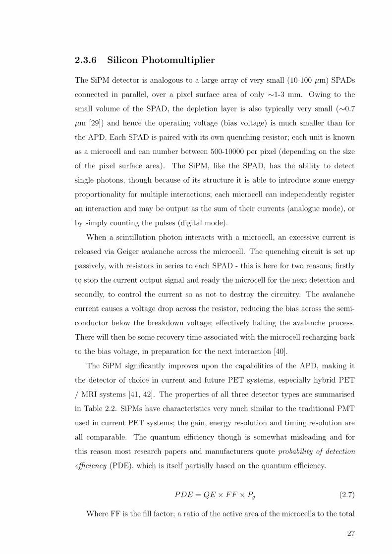
2.3.6 Silicon Photomultiplier
The SiPM detector is analogous to a large array of very small (10-100 µm) SPADs
connected in parallel, over a pixel surface area of only ∼1-3 mm. Owing to the
small volume of the SPAD, the depletion layer is also typically very small (∼0.7
µm [29]) and hence the operating voltage (bias voltage) is much smaller than for
the APD. Each SPAD is paired with its own quenching resistor; each unit is known
as a microcell and can number between 500-10000 per pixel (depending on the size
of the pixel surface area). The SiPM, like the SPAD, has the ability to detect
single photons, though because of its structure it is able to introduce some energy
proportionality for multiple interactions; each microcell can independently register
an interaction and may be output as the sum of their currents (analogue mode), or
by simply counting the pulses (digital mode).
When a scintillation photon interacts with a microcell, an excessive current is
released via Geiger avalanche across the microcell. The quenching circuit is set up
passively, with resistors in series to each SPAD - this is here for two reasons; firstly
to stop the current output signal and ready the microcell for the next detection and
secondly, to control the current so as not to destroy the circuitry. The avalanche
current causes a voltage drop across the resistor, reducing the bias across the semi-
conductor below the breakdown voltage; effectively halting the avalanche process.
There will then be some recovery time associated with the microcell recharging back
to the bias voltage, in preparation for the next interaction [40].
The SiPM significantly improves upon the capabilities of the APD, making it
the detector of choice in current and future PET systems, especially hybrid PET
/ MRI systems [41, 42]. The properties of all three detector types are summarised
in Table 2.2. SiPMs have characteristics very much similar to the traditional PMT
used in current PET systems; the gain, energy resolution and timing resolution are
all comparable. The quantum efficiency though is somewhat misleading and for
this reason most research papers and manufacturers quote probability of detection
efficiency (PDE), which is itself partially based on the quantum efficiency.
PDE = QE × FF × Pg (2.7)
Where FF is the fill factor; a ratio of the active area of the microcells to the total
27

area of the SiPM and accounts for the dead space present between micropixels. Is
intrinsically linked to the geometrical design of the microcell array; typical values
range from 20-80% [29, 43, 44]. Pg is the probability of an electron-hole pair causing
an avalanche event and is dependent upon the location of the interaction (and hence
primary electron-hole pair) and the electrical field shape [45] - typical values range
between 0.5-1 [29, 46]. Generally, the combination of these factors leads to an
overall PDE of much less than 100 %, especially for shorter wavelengths (since QE
is strongly wavelength dependent). Usually this will be in the vicinity of 30-40%,
though has been reported as high as 55% at 420 nm [23, 47, 48] - interestingly still
higher than PMTs.
TOF PET is a very active area of research at present and SiPMs have proven
to be aligned to this goal [7]. There are certain traits which are being explored
further to improve the intrinsic timing resolution. Improving the PDE is one avenue;
higher detection probability means that there is a higher chance that the very first
scintillation photons will be detected. Reduction in the SiPM capacitance is another
avenue; a large SiPM capacitance increases both the rise and decay times of the
pulse. This is actually tied to the size of the microcell surface area, though simply
decreasing the size of the microcells presents a compromise in PDE, as the proportion
of dead space between pixels will be increased. Progress is being made on new
fabrication techniques which are being used to reduce the gap between microcells,
while minimising the amount of optical crosstalk (this is itself a problem, as a photon
detection can effectively be doubled by neighbouring microcells) [23, 48, 49]. SiPMs
are already very competitive, if not superior to both PMTs and APDs, despite their
relatively short time in the field - further improvement of their performance as well
as reductions in fabrication cost will mean it is only be a matter of time before other
photodetectors are completely supplanted.
2.3.7 Detector Designs
Block Scintillation Detectors
Modern PET systems in the current clinical environment incorporate a block scin-
tillation detector design. Traditional scintillation detectors have aimed to locate the
position of the annihilation photon by restricting the scatter of scintillation photons
28

Properties PMT APD SiPM
QE (%) 20-30 >80 >80
PDE(%) 30 @320 nm 74 @600 nm 55@ 420 nm
Single Photon Response Yes No Yes
Gain 106-107 102-103 106-107
Temp. Dependence Low High Medium
B Field interaction Yes No No
Energy Resolution (%) 15-25 16.2 19-25
Timing Resolution (ns) 0.475 26-43 0.24
Table 2.2: A comparison of typical photodetector properties.
within a small volume. In this case, the spatial resolution is therefore proportional to
the size of the detector. The block detector reduces the size of the crystal elements
by cutting the block into a grid array and then filling the gap with highly reflective
material to stop optical photons being transmitted to neighbouring elements.
Before the block detector was introduced each detector element would have it’s
own PMT, but costs could quickly blow out if this method were continued whilst
trying to reduce detector size. The solution was to use a number of PMTs for each
block (for example using a 2×2 array of PMTs for a block of 8×8 crystal elements),
then using Anger logic to locate the position of the annihilation event. This system
has been further improved by using quadrant sharing, which uses larger sized PMTs
to overlap adjacent blocks allowing the number of PMTs to be further reduced.
More recent systems have incorporated digital SiPMs rather than PMTs.
Problems with this design still remain though; there is still an element of inter-
crystal light scatter, especially for high resolution systems where crystal size is very
small (on the order of 1 cm length by 1 mm×1 mm face). There is also a compromise
between having good depth of interaction (DOI) information (short crystals) or high
sensitivity (long crystals). There are some designs that have attempted to address
this, but generally there will be a cost involved as other performance parameters are
reduced [50]. Figure 2.7 shows a number of alternative designs which use depth en-
coding to address the DOI issue, though in most of these designs (all except for (d)
- the monolithic detector, and (a) in some cases [51, 52]) estimation of the position
29

of interaction is somewhat limited; being localised to only two possible depths. A
high DOI uncertainty leads to what is known as parallax error or DOI blurring in
the acquired images; the LOR may be drawn incorrectly from the inner face of the
scintillator material, rather than the actual position. This problem becomes more
pronounced the further the LOR is from the central axis of the detector, meaning
that there will be non-uniform spatial resolution across the field of view.
The subfigures in Figure 2.7 provide depth encoding via a number of methods;
(a) simply by stacking two (or more) crystal / photodetector units and reading each
layer independently [53, 54, 55], (b) dual-end photodetectors which provide DOI in-
formation by analysing the difference in light intensity at each end (simultaneously)
[56, 57, 35, 58], (c) Phoswich configurations which use layers of crystals with differ-
ent decay characteristics and determine DOI via pulse shape discrimination [59, 60,
61], (d) monolithic crystals which use statistical modelling of light maps incident
on the detector surface [62, 50, 63, 64, 65], or (e-f) dual-layer crystals with offset
positions or mixed shapes, which have different light output profiles [66, 67]. More
recently, other solutions to depth encoding have emerged which utilize a light guide
at the entrance face of the scintillator crystal. These light guides mimic a dual-sided
detector readout by redirecting light travelling away from the photodetector back
towards it, along non-primary elements [68, 69, 70].
The sensitivity of the system is reduced because of the dead space introduced by
the reflective material between detector elements. And although it is not related to
performance, the cost of manufacture will increase for smaller sized crystals, due to
the complexity and scale of machining needed.
Monolithic Scintillation Detectors
One particularly interesting solution to DOI blurring is monolithic scintillators.
These use the light intensity and spread of scintillation photons on the photode-
tector pixels to estimate the position of the scintillation event and unlike the block
detector, the spatial resolution is not dependent on the size of the crystal. They also
have improved gamma photon capture efficiency, and have good spatial and energy
resolution [72, 73, 62].
Many different methods have been proposed to determine the point of interac-
30

(a) (b) (c)
(d) (e) (f)
Figure 2.7: Detector designs seeking to improve upon the DOI capabilities of the
block detector. (a) Dual-crystal photodetector(s) layers. (b) Single-crystal layer
with photodetectors at each end. (c) Phoswich design with two types of scintillation
materials. (d) Statistical positioning with a monolithic crystal block. (e) Dual-layer
crystals with offset positions. (f) Dual-layer crystals of mixed shapes. [71].
tion between an incident gamma photon and a monolithic scintillators based on
analysis of the distribution of optical photons detected on one or more surfaces of
the monolithic slab.
Statistical algorithms such as maximum likelihood (ML) [74, 75], chi-squared
(χ2) [72] or k-nearest-neighbour kNN [72, 62, 76] have been used to fit the optical
photon distribution, as measured by the optical photodetector, to a set of previously-
measured reference profiles, and thereby estimate the 3D point of interaction within
the crystal. These algorithms have been shown to work well; however, the calibration
of the localisation systems (i.e. the production of the reference profiles) requires
either laborious experimental measurements or extensive Monte Carlo simulations,
31

since a large number of events must be recorded over a range of known positions
and angles of incidence. This work would also need to be repeated for monolithic
slabs with different dimensions or material properties.
An alternative to the statistical methods is to fit an analytic function to the
observed optical photon distribution, using an optimisation algorithm which aims to
minimise the mean squared error between the observed distribution and the analytic
model [63, 77]. Where an exact analytic model is difficult or impractical to derive
due to complex optical properties of the material or the presence of high levels
of Rayleigh scatter, neural networks may offer superior performance as they can
intrinsically account for non-linearities in the relationship between the observed
photon distribution and the point of interaction in the slab, particularly near slab
boundaries. [78].
The optical photon distribution observed at the detector surface may be affected
by internal reflections from the sides of the slab, and may be truncated near its edges
and corners, which will impair the performance of analytic-model-based position
determination algorithms unless incorporated into the model. Covering the non-
detector faces of the scintillator slab with an absorptive coating, such that optical
photons reaching the edges of the slab will be absorbed rather than reflected, allows
the model to be simplified, at the cost of some sensitivity. Such coatings are known
to degrade energy resolution to some extent; however, this can be mitigated if the
scintillator has a high scintillation yield [72, 77].
The optical photon distribution which will be observed depends on the nature
of the interaction of the gamma photon with the scintillator. For cases where the
photon is photoelectrically absorbed, all of the optical photons will be emitted from
a single point, with the number of optical photons proportional to the energy of
the gamma photon. A similar outcome will result from Compton interactions where
the scattered photon escapes from the scintillator slab; in this case, the number of
photons emitted at the point of interaction will be proportional to the difference
in energy between the incident and scattered photon. These two cases will be the
easiest to localise due to the simplicity of the interaction; the scintillation event
may be treated as an isotropic point source [77, 78]. In a scattering medium, it is
necessary to also introduce an attenuative factor due to the imperfect transparency
32

of the material [79]. This is described by (2.8)
J =ε
4πR2e−kR (2.8)
where J is the flux density of optical photons at distance R from a source emitting
ε photons following a scintillation event. The scatter-induced losses are modelled
by k.
In the event of multiple points of energy deposition within the scintillator (for ex-
ample, a Compton interaction followed by photoelectric absorption of the scattered
photon), the optical photon distribution becomes much more diffuse, and accurately
fitting an analytic model to the observed optical photon distribution becomes a much
more difficult problem. If individual pulses can be discriminated, it may be possible
to estimate each location where energy was deposited in the scintillator. For PET,
only the first of these is important, since this will define the endpoint of the line of
response. This is most likely to be the shallowest observed scintillation event.
2.3.8 Alternative Detector Configurations
Typical PET scanners used in the clinical environment feature 4-5 full rings of block
scintillation detectors, surrounding the patient. The axial field of field of view is
typically 15-25 cm [2]. Several groups have attempted to expand the axial or solid
angle coverage of PET scanners to improve the sensitivity of the system and hence
the image signal to noise ratio. Cherry et. al. are developing perhaps the most
high profile system regarding this: the “EXPLORER” project is a long axial “total
body” system, capable of imaging the entire body at once [4].
Other attempts to improve the solid angle coverage include the development of
full body truncated spherical systems [80], or partial spherical or polyhedral systems
for targeted brain scans[81, 82]. Though most of these designs have proven difficult
to construct and have remained theoretical studies.
Systems consisting entirely of monolithic scintillation detectors [65] reduce the
amount of dead space, while simultaneously improving DOI estimation. A small
animal system featuring a continuous cylindrical slab of LYSO scintillator has been
constructed [83], which has been shown to achieve good spatial resolution and sen-
sitivity. Though the method of construction has been achieved by boring a hole in
33

the centre of a single crystal ingot, so scalability may prove challenging.
Increasing the geometric coverage of the scanner will positively influence the
signal-to-noise ratio, spatial resolution and reduce scan time (or alternatively the
radiation burden on the patient). Generally though, an increase in component cost
scales with the increase in coverage [23].
2.3.9 Time-of-Flight PET
In recent years there have been significant advances in the timing resolution of PET
detectors, thanks to the discovery of fast scintillation materials (such as LSO, LYSO
and LaBr3) and the advancement of photodetectors (especially SiPMs) [84, 7]. In
modern PET systems, timing resolution has reached below the nanosecond range,
with detectors now able to distinguish between singles events which are hundreds
of picoseconds apart. The measured time difference (∆t) between the two singles
correlates to the position (∆x) of the annihilation event with respect to the central
axis of the ring structure (see Figure 2.8), according to the equation [85]
∆x =c∆t
2(2.9)
Theoretically, if coincidence timing were exactly precise, it would be possible to
pinpoint the exact location of the annihilation event and there would be absolutely
no need for image reconstruction. In reality, a fast timing resolution is able to
reduce the size of the LOR to a probable range. The time difference (∆t) is blurred
by variance σ2∆t, which corresponds to a blurring of the estimated position by σ2
∆t
(this variance is show in Figure 2.8).
More certainty in the position of the annihilation event, along the LOR translates
to less influence from random and scatter events and an overall improvement of
the signal-to-noise ratio [23, 86]. Also beneficial, is an increased accuracy of the
attenuation map and the possibility of generating an attenuation map based on
emission data [87, 88, 89, 90, 91].
Time-of-flight detectors, which also use depth encoding to provide DOI infor-
mation, can actually improve the timing resolution further by adding a timing cor-
rection to the signal, accounting for the propagation time of scintillation photons
through the medium [7, 92]. Monolithic scintillation detectors have an additional
34
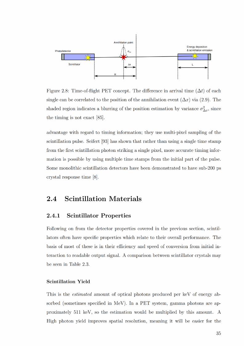
D x
R
s D x
S ci ntill at or
P h ot o d et e ct or
A n ni hil ati o n p oi nt
E n er g y d e p o siti o n
& s ci ntill ati o n e mi s si o n
L
Fi g ur e 2. 8: Ti m e- of- fli g ht P E T c o n c e pt. T h e di ff er e n c e i n arri v al ti m e ( ∆ t) of e a c h
si n gl e c a n b e c orr el at e d t o t h e p ositi o n of t h e a n ni hil ati o n e v e nt ( ∆ x ) vi a ( 2. 9). T h e
s h a d e d r e gi o n i n di c at es a bl urri n g of t h e p ositi o n esti m ati o n b y v ari a n c e σ 2∆ x , si n c e
t h e ti mi n g is n ot e x a ct [ 8 5].
a d v a nt a g e wit h r e g ar d t o ti mi n g i nf or m ati o n; t h e y us e m ulti- pi x el s a m pli n g of t h e
s ci ntill ati o n p uls e. S eif ert [ 9 3] h as s h o w n t h at r at h er t h a n usi n g a si n gl e ti m e st a m p
fr o m t h e first s ci ntill ati o n p h ot o n stri ki n g a si n gl e pi x el, m or e a c c ur at e ti mi n g i nf or-
m ati o n is p ossi bl e b y usi n g m ulti pl e ti m e st a m ps fr o m t h e i niti al p art of t h e p uls e.
S o m e m o n olit hi c s ci ntill ati o n d et e ct ors h a v e b e e n d e m o nstr at e d t o h a v e s u b- 2 0 0 ps
cr yst al r es p o ns e ti m e [ 8].
2. 4 S ci n till a ti o n M a t e ri al s
2. 4. 1 S ci n till a t o r P r o p e r ti e s
F oll o wi n g o n fr o m t h e d et e ct or pr o p erti es c o v er e d i n t h e pr e vi o us s e cti o n, s ci ntil-
l at ors oft e n h a v e s p e ci fi c pr o p erti es w hi c h r el at e t o t h eir o v er all p erf or m a n c e. T h e
b asis of m ost of t h es e is i n t h eir e ffi ci e n c y a n d s p e e d of c o n v ersi o n fr o m i niti al i n-
t er a cti o n t o r e a d a bl e o ut p ut si g n al. A c o m p aris o n b et w e e n s ci ntill at or cr yst als m a y
b e s e e n i n T a bl e 2. 3.
S ci n till a ti o n Yi el d
T his is t h e e sti m at e d a m o u nt of o pti c al p h ot o ns pr o d u c e d p er k e V of e n er g y a b-
s or b e d (s o m eti m es s p e ci fi e d i n M e V). I n a P E T s yst e m, g a m m a p h ot o ns ar e a p-
pr o xi m at el y 5 1 1 k e V, s o t h e esti m ati o n w o ul d b e m ulti pli e d b y t his a m o u nt. A
Hi g h p h ot o n yi el d i m pr o v es s p ati al r es ol uti o n, m e a ni n g it will b e e asi er f or t h e
3 5

ScintillatorDensity Yield Decay Peak λ R
Zeff Hygro Refs.(gcc) (/keV) (ns) (nm) (%)
NaI:Tl 3.67 45 230 415 7.1 50 Yes [94, 10]
BGO 7.13 8 300 490 11 73 No [95, 10]
LSO:Ce 7.4 27 40 420 7.9 66 No [96]
LYSO:Ce 7.1 34 41 397 8.1 65 No [97]
GSO:Ce 6.7 12.5 56 430 7 59 No [96]
LuAp:Ce 8.34 11.4 16.5 365 9.3 65 No [95]
LaBr3:Ce 5.1 63 16 380 2.6 46 Yes [98]
LaF3:Ce 5.9 4.5 30 330 16 - Yes [94]
YAG:Ce 4.57 24 88 550 11.1 32 No [99]
Plastic* 1.03 10 2 Various - 12 No [10]
Table 2.3: Some common scintillation materials used in PET detectors. * Indicates
typical values — there are many different types of plastic scintillators. Energy
resolution (R) is measured at a reference energy of 662 keV. Some scintillators are
identified by their acronyms: Bi3Ge4O12 (BGO), Gd2SiO5:Ce (GSO:Ce), Lu2SiO5:Ce
(LSO:Ce), LuAlO5:Ce (LuAP:Ce), Lu1.8Y0.2SiO5:Ce (LYSO:Ce)
.
exact location of the hit to be determined. This is especially useful in PET sys-
tems where the scintillation photons are spread between multiple photo-detectors,
or in monolithic scintillation detectors where a high photon yield translates to high
statistical accuracy [77].
Decay Time
Refers to the amount of time required for light photons to be produced by the
scintillator. A fast decay time is necessary for timing precision (and is a requirement
for TOF PET) and also ensures that events do not “pile up” on top of one another,
causing dead time in the detector. A good scintillator is able to process events at
high count rates, while reducing the amount of random coincidences. As a general
rule of thumb, for a scintillator decay time τ , the maximum event rate that the
scintillator can handle is1
2τ[10].
36

Am
plitu
de
Time
tscintillator decay
Figure 2.9: Typical scintillator pulse shape. [85].
It is also important to note that for systems dependant upon very precise timing
resolution (i.e. TOF PET), the rise time of the scintillator is also a very important
consideration. Time stamping of a coincidence event will generally happen when
optical photon detection reaches above a certain threshold, which is achieved during
the rising portion of the pulse (see Figure 2.9). Fast crystals, such as LSO, LYSO
and LaBr3, tend to have both fast rise and decay times.
Emission Wavelength
The frequency spectrum of the scintillation photons should be matched to the spec-
tral efficiency of the photodetector. For example, a typical photomultiplier tube
with a bi-alkali photocathode has an optimal spectral peak between 350 nm – 475
nm. If the peak is too far below 350 nm (i.e. UV range), then there is a chance
that the scintillation photons will be absorbed into the glass in the entrance of the
photodetector.
37

Index of Refraction
This parameter is important for coupling light from the scintillator to the photode-
tector. Ideally, the refractive index of the scintillator needs to match the refractive
index of the glass on the photodetector to reduce internal reflections. This is also
relative to the emission wavelength of the scintillation photons.
Optical Attenuation Length
This is somewhat different to the stopping power mentioned previously in the section
on detector properties. For high energy gamma photons, a material possessing a
low attenuation length (high stopping power) is desirable, so there is maximum
probability of the photon interacting with the material (this depends on ρ and
Zeff ). In the optical range however, the reverse is true. Scintillators with a long
optical attenuation length are preferred for better energy resolution, or in the case
of monolithic detectors; to more accurately execute positioning algorithms.
The attenuation length (λ) is defined as the length of penetration (y) where the
irradiance (I(y)) has dropped to 1/e of the incident irradiance (I0). Often material
datasheets will specify an attenuation or absorption coefficient (α), rather than an
attenuation length - though this is just the inverse (i.e. λ = 1/α). (2.10) shows the
relation in terms of the attenuation coefficient [100]
I(y) = I0e−αy (2.10)
It should easily be seen that for y = 1/α, the irradiance has dropped to e−1 of I0.
In addition to these properties it is most desirable for scintillators to be rugged, cheap
to manufacture and non-hygroscopic (meaning it will not absorb water molecules).
There are many different types of scintillation materials which have been used
in PET systems, though in almost all cases these will be inorganic crystals, owing
mostly to superior stopping power and scintillation yield (despite expensive and
time consuming fabrication processes). Plastic scintillators, such as polystyrene,
polyvinyltoluene (PVT) or polymethylmethacrylate (PMMA) with an added fluor
can produce acceptable yield and exceptional timing resolution for PET applications,
they are also easily shaped and cheap to produce. However, the stopping power is
38

much too low comparatively and they are particularly susceptible to damage from
high energy gamma photons [101].
2.4.2 Nanocomposite Scintillators
Nanocomposite scintillators are a relatively new class of materials for radiation de-
tection applications. They consist of a mixture of nanometre-scale (most commonly
inorganic) scintillating particles, uniformly mixed with a transparent polymer or
other organic matrix. The matrix can either be non-scintillating, such as oleic acid
(OA), or a polymer scintillator, such as polystyrene (PS) or polyvinyltoluene (PVT).
Because the gaps between scintillator nanoparticles are filled with a material with
a refractive index closer to that of the scintillator than air (or vacuum), scattering
is limited and light transmission is improved compared to the use of a compressed
bulk powder [102]. Nevertheless, no matrix material has a refractive index which
perfectly matches that of the nanocrystal; therefore, scattering remains a significant
performance-limiting factor, particularly in comparison to monocrystalline scintilla-
tor materials. For hygroscopic materials, the matrix offers the additional advantage
of providing a degree of protection for the nanoparticles against moisture ingress.
Some examples of nanocomposites which may be feasible for PET have been sum-
marised in Table 2.4.
Accurately modelling the optical and physical properties of a nanocomposite is
considerably more complex than for a homogeneous material. Scattering may be
approximated as Mie scattering, but since the particle size is normally much smaller
than the nanocrystal scintillator’s emission wavelength, it may be assumed that each
particle will see an approximately uniform electric field. Therefore, scattering can
be approximated as purely Rayleigh to a high degree of accuracy [94].
Most useful nanoscintillator particles will be of a size such that scattering is
essentially purely Rayleigh (i.e., satisfying the criteria m · x < 1, where m = np/nm
is the ratio of the refractive index of the scintillator particles to that of the matrix,
and x = 2πr/λ and λ = λ0/nm where λ0 is the peak emission wavelength of the
scintillator [105]). If this condition is satisfied, then the transmission of scintillation
39

Nanoparticle LaBr3:Ce Gd2O3 LaF3:Ce LaF3:Ce YAG:Ce
Matrix PS PVT OA PS PS
Load (% Vol.) 19 4.6 34 50 50
Peak λ (nm) 380 550 334 334 550
Yield (ph/keV) 63 22 4.5 4.5 20.3
R (% @662 keV) 2.6 11.4 16 16 11.1
Decay (ns) 16 17 30 30 87.9
ρ (g/cm3) 1.81∗ 1.34∗ 2.59∗ 3.47∗ 2.81∗
n (@peak λ) 1.69∗ 1.56∗ 1.52∗ 1.65∗ 1.72∗
α (cm−1) 2.00∗ 0.09∗ 2.05∗ 0.15∗ 0.95∗
Refs. [98, 103] [21, 103] [104, 94, 103] [104, 94, 103] [99, 103]
Table 2.4: Physical and optical properties of a range of proposed nanocomposite
materials. Most properties listed are found from the literature; several parameters,
marked with an ∗, have been estimated from the volume fractions listed, assuming
a 1 cm thick slab with 9 nm diameter nanoparticles. R is the loading factor. PS is
polystyrene; PVT is polyvinyl toluene; OA is oleic acid.
photons may then be calculated via (2.11) [94, 21, 106, 107]:
T =I
I0
= exp
{−4π4d
3Lfpn4m
λ4
(m2 − 1
m2 + 2
)2}
(2.11)
Where I/I0 is the ratio of the output light intensity (I) to the emission light
intensity (I0), d is the diameter of the nanoparticle, fp is the volume fraction of
particles, L is the average path length and λ is the wavelength of the scintillation
photons. This expression assumes that the diameter of nanoparticles is uniform,
there is no agglomeration of particles in the matrix, also that the photons emitted
during scintillation are of exactly the same wavelength.
In practice, none of these assumptions is strictly accurate. Particle agglom-
eration is of particular concern where the nanocomposite loading factor is high,
potentially creating additional scattering losses [108]. If there is some overlap be-
tween the absorption spectrum of the matrix and the luminescence spectrum of the
nanoscintillator, self-absorption of scintillation photons may occur; some polymer
matrix materials are known to exhibit this behaviour, especially in the UV region
40
[21, 109]. Despite these limitations, (2.11) provides a good approximation of optical
transmission of scintillation photons for the majority of nanocomposite materials.
The refractive index of the nanocomposite (nc) is a function of the nanoparticle
loading factor - in fact, much research has been conducted into the problem of using
inorganic nanoparticles to effectively tune the refractive index of an organic material.
Generally, an effective medium model based on Maxwell-Garnett theory (or variants
of it) can be used to estimate the composite refractive index using an additive linear
approximation, as shown in (2.12) [110, 111, 112]
nc = nmfm + npfp (2.12)
Where nm and np are the refractive indices of the matrix and nanoparticles re-
spectively and fm and fp represent the fractions of each material, by volume. It
is important to note that while a large number of inorganic-organic nanocomposite
scintillator materials are known to follow this linear relationship between volume
fraction and overall refractive index, others do not. There are a number of different
factors which affect the refractive index; unfortunately, there is no general theoreti-
cal model which can be applied to all combinations of materials. Instead, it is often
necessary to employ empirical methods. For instance, a TiO2-polystyrene nanocom-
posite synthesised by Rao et. al [113] is best described by a quadratic equation.
The authors hypothesise that strong chemical bonding between the two materi-
als changed the polarisability of the polymer, resulting in the observed behaviour.
Other factors which can impact upon the refractive index include the diameter of
the nanoparticles; for PbS-gelatine, there was a significant drop in refractive index
compared to the bulk material when the mean diameter of the nanoparticle compo-
nent was less than 25 nm [112]. Also, if a surfactant coating with a lower refractive
index than the nanoparticle is applied to improve the uniformity of the nanocom-
posite, it may significantly contribute to the overall volume [114] and hence alter
the refractive index.
Using (2.11) and (2.12), it is possible to get a sense of the desirable properties
for suitable bulk scintillator and matrix materials. Ideally, closely matching scintil-
lator and matrix refractive indices, small nanoparticle size (< 10 nm), long emission
wavelength and non-overlapping emission and absorption spectra will help to max-
41

(a) Calculated optical attenuation length from Rayleigh scattering, using (2.11).
(b) Calculated gamma HVL thickness as a function of scintillator loading factor.
Figure 2.10: (a) All nanoparticles are assumed to be spherical and uniformly dis-
tributed, with a constant diameter of 9 nm (for comparison). (b) Calculated using
data from the National Institute of Standards and Technology [103].
42

imise transmission of the scintillation light. For the bulk scintillator material, high
light yield per MeV of incident photon energy, good energy resolution, and a short
time constant are also desirable for most applications.
In addition to these desirable properties, the nanocomposite needs to exhibit a
high linear attenuation coefficient so as to maximise its sensitivity to high-energy
gamma radiation. This requires the nanocomposite to have as high a density and
effective atomic number as possible. Since these properties are generally quite low
for the matrix material, it is necessary to use a high-ρ, high-Zeff bulk scintillator
material at a high loading factor. Unfortunately, a high loading factor also has
the effect of reducing the optical transmittivity of the nanocomposite. This can
be more easily seen in Figure 2.10(a), which uses (2.11) to calculate the optical
attenuation length of for a number of potential nanocomposite materials, and Figure
2.10(b), which compares the half-value layer (HVL, sometimes referred to as half
value thickness, defined as the thickness required to reduce the intensity of incident
gamma radiation by 50%) for each material as a function of loading factor (volume
fraction of scintillator).
2.4.3 Transparent Ceramic Scintillators
Doped synthetic garnet materials, such as yttrium aluminium garnet (YAG) and
lutetium aluminium garnet (LuAG) have been been used for decades in monocrys-
talline forms in photonics applications such as optically pumped lasers. Monocrys-
talline synthetic garnet scintillators have also been proposed for use in a variety of
medical imaging applications such as PET due to their high density, high scintilla-
tion yield and good optical transparency. Recent progress in fabrication techniques
has enabled the synthesis of certain garnets as optically transparent polycrystalline
ceramics. Such ceramics retain many of the properties of the equivalent monocrys-
talline material (in particular, the high density and linear attenuation coefficient),
and may offer a higher scintillation yield in some cases [115]). The principal benefit
of multicrystalline transparent ceramics is easier and more cost-effective fabrication,
and the flexibility of being able to form the precursor powder into arbitrary shapes
and structures prior to sintering - a near-impossibility with single-crystal materials.
The optical and scintillation properties of transparent ceramics are heavily in-
43

Ceramic GYGAG:Ce GLuGAG:Ce GAGG:Ce LuAG:Pr
Peak λ (nm) 550 550 530 310
Yield (ph/keV) 50 48.2 70 21.8
R (%) 4.9 7.1 4.9 4.6
1st Decay (ns) 100 84 90 21.4
2nd Decay (ns) 500 148 194 771
ρ (g/cm3) 5.8 6.9 6.63 6.73
n (@peak λ) 1.82 1.92 1.90? 2.03?
α (cm−1) 0.10 2.00 3.13∗ 2.86∗
refs. [119, 120, 121] [118, 84] [115, 122] [117, 122]
Table 2.5: Properties of several transparent ceramic scintillator materials proposed
for radiation detection applications. Properties listed with ∗ have been calcu-
lated, while those with ? were obtained from literature pertaining to the equivalent
monocrystalline form of the material.
fluenced by the specific manufacturing process used. Usually, the ceramic is formed
by the sintering method, where a precursor material is calcinated and milled into
nanoparticles (∼100-200 nm) before being pressed into a green body (unfired ce-
ramic) and sintered at around 1500-1700◦C [116, 117]. The resulting solid may then
undergo hot isostatic pressing (HIP) to reduce porosity, followed by annealing and
polishing to create a highly transparent solid [118, 119]. The atmosphere in which
the sintering and annealing steps are performed has a significant effect on the trans-
parency of the resulting ceramic, and its propensity to exhibit afterglow effects [120].
The properties of several examples of ceramic garnet scintillators are listed in Table
2.5.
Compared to the Czochralski, Kyropoulos or Bridgman-Stockbarger methods
used to grow large single-crystal scintillators, the process of creating transparent ce-
ramic scintillators is much more amenable to the production of complex geometries
and scaling up to large volumes. Growth of high-quality defect-free monocrystalline
scintillators with consistent characteristics requires extremely high, uniform and
well-regulated temperatures and atmospheric conditions. Additionally, the maxi-
mum dimensions of monocrystalline scintillators are limited by both the maximum
44

dimensions of the ampoules (in the Bridgman-Stockbarger method) and by the diffi-
culty in maintaining a stable, uniform thermal gradient across a wide crystallisation
zone [26, 27]. The ability of the ceramics to be pressed into different moulded shapes
eliminates most of these problems, and the lower temperatures involved mean that
material losses are able to be more easily controlled since there is no risk of evapo-
ration of the melt.
One of the most significant challenges of producing ceramic garnet scintillators is
achieving high optical transparency in the finished product. Cherepy et al. proposed
a method to reduce the residual porosity of the ceramic with hot isostatic pressing,
greatly improving optical transparency [121]. Optical properties are also improved
through the selection of high purity precursor materials with cubic / isotropic crystal
structures (i.e. no birefringence), which reduces optical scatter caused by grain
boundaries and secondary phases [121].
2.5 Image Reconstruction
A major underlying problem with PET is that the radiotracer distribution inside
the patient cannot be directly imaged. Instead, the image must be reconstructed
by first taking the measured LOR data and then applying an algorithm to convert
1D projection data (or list-mode data) into a 2D or 3D image. There are two broad
groups of algorithms used for image reconstruction: analytic image reconstruction,
which is based on a mathematical analysis of the Radon transform, or iterative re-
construction which is based on least squares or expectation maximization algorithms
converging to an image.
2.5.1 Data Storage
Sinograms
In image processing, it is generally accepted to describe lines in the image space in
terms of normal parameterisation [123], so the LORs used for the projection data
p(s, φ) will often be defined as shown in Figure 2.11. The parallel LORs at a singular
projection angle φ (the angle subtended by the normal to the LOR with respect to
the x-axis), are shown as the dashed lines a distance s from the origin; described in
45

Sinogram
s
φ
φ
x
y
sp(s, φ)
f(x, y)
Integration along allLORs at fixed φ
Figure 2.11: Construction of a sinogram from projection data [125]. The dashed
lines are measured lines of response from a particular projection angle. The Radon
transform is then used to obtain a 1D intensity distribution, which is then stored in
the sinogram as a function of distance and projection angle.
this coordinate system by the equation
x cosφ+ y sinφ = s (2.13)
The projection p(s, φ) is obtained by taking a line integral along each LOR, to
give an intensity profile at that particular angle. This operation is known as the
(2-D) Radon transform [124], or the x-ray transform and is written as
p(s, φk) =
∞∫−∞
∞∫−∞
f(x, y) δ(x cosφ+ y sinφ− s) dx dy (2.14)
Where f(x, y) is the object being imaged; in this case the radiotracer distribution
inside the patient. Essentially, integration across the object only occurs when the
argument of the delta function (x cosφ+y sinφ) is equal to zero (i.e. for a particular
s value corresponding to a measured LOR). In Figure 2.11 represents a continuous
function, though in real world applications, the projections will be discretised as
they are dependent upon discrete LORs. It is therefore more appropriate in this
case to describe the projections as double sum equations, rather than integrals.
46
Each of these projections are then stored in a sinogram, as shown in Figure 2.11.
Each row of the sinogram corresponds to a particular projection, with each point
along the s plane represented by a particular intensity value. This is then repeated
for each projection angle until the entire 180° range of measurements are covered (the
LORs extend in both directions, so measurements > 180° will be redundant). Each
point of the object’s radiotracer intensity distribution is represented as a sinusoid.
List Mode Data
An alternative to sinogram storage is list mode data collection. Rather than plot
each projection on a graph, each capture is simply listed as an entry into a data
file. The advantage of this methodology is that parameters other than position may
be recorded at the same time. It is especially useful to record energy and timing
information of coincidences, for simplicity in filtering scattered photons and random
coincidences, through the application of energy and timing windows. In fact, this
methodology has produced improvements in spatial and temporal accuracy [87, 126,
127]. Additionally, timing information may be used for TOF PET. This method does
require a large amount of storage space however, especially for data capture in high
resolution, high sensitivity systems, where each event requires a separate data entry.
As hard drive storage naturally is becoming cheaper and faster, this should be less
of a problem moving forward.
2.5.2 Filtered Backprojection
Analytic image reconstruction attempts to find the solution to the inverse Radon
transform, for each projection. The result of simple backprojection will look like a
“smearing” of the projection across the 2-D image space, with each of the projection
intensity values being spread uniformly over the image pixels which lie along the
LOR at that particular angle. As each of the backprojections are overlaid onto the
pixels, they will overlap, causing a blurring of the image from oversampling. This
effect is commonly known as 1/r blurring, where r represents the distance from the
object of interest.
The blurring may be understood by looking first at how the projection data
relates back to the final image. The central section theorem tells us that the 1D
47

Fourier Transform (FT) of a projection at angle, φ, will equal the cross section of the
2D FT of the image at the same orientation [9]. Therefore, the 2D FT of the image
will have a superposition of all 1D FT projection data and will be oversampled about
the centre (looking like spokes on a wheel). A Fourier analysis reveals that a filter
function is required for correction. The image f(x, y) of the radiotracer distribution
of the original object may be described as
f(x, y) =
π∫0
∞∫−∞
|νs|P (νs, φ)ej2πsνs dνs dφ (2.15)
The inner integral in (2.15) is therefore simply the inverse Fourier transform
of P (νs, φ) multiplied by a filter function with frequency response |νs|. This is
called filtered backprojection. Reconstructing the entire image from these filtered
back projections requires integration of all filtered backprojections over the range
0 < φ < π.
In practice, the process for filtered backprojection is as follows [128]:
� Take the 1D Fourier transform of each projection p(s, φ) to give P (νs, φ).
� Multiply P (νs, φ) by the filter function |νs|.
� Take the 1D inverse Fourier transform.
� Integrate over the range 0 < νs < π to get a reconstruction of f(x, y) (simple
backprojection).
The filter function |νs| we are talking about here is a ramp function, which is
actually not absolutely integrable; as the integral would tend towards infinity. Also,
because |νs| = 0 at νs = 0, some information may be lost at this point of the
algorithm. Often this value will be scaled or a simple guess to account for this. A
number of functions have been developed to address these issues, perhaps the most
basic of which is the“Ram-Lak” filter [129], which is essentially a ramp function that
has been band limited to the maximum frequency measurable in a projection (see
Figure 2.12). That is, we use a windowed filter function.
The maximum frequency of the filter is known as the Nyquist frequency and may
be easily determined if the pixel size is known for a particular detector. Because the
48

acquisition data are discrete, the maximum number of peaks possible in a projection
would be in a situation in which peaks and valleys occur in every alternate pixel
[130]. The Nyquist frequency can then be determined by the simple formula
Nyquist Frequency =0.5 cycles
pixel size (cm)(2.16)
If sampling is coarser than the Nyquist rate, then too many of the higher spatial
frequencies may be cut out leading to image artefacts, known as aliasing.
2.5.3 Backproject Then Filter
Another technique which attempts to remove 1/r blurring is the Backproject Then
Filter algorithm (BPF). This is similar to FBP, but the filter is applied at a different
stage in the process; whereas in FBP the filter is applied before backprojection, in
BPF it is applied after.
This can overcome some of the added complexity of FBP in terms of necessary
rebinning and interpolation, but generally the images are poorer in quality and
the process is more computationally intensive. This is primarily caused by the
backprojection process generating an image that is beyond the original matrix size;
the 2D blurred image must be truncated to the size of the original, losing data in
the process [131]. Using 2D Fourier transforms with a cone filter may also produce
periodic convolution, causing wrap around effects [132]. For these reasons FBP has
proven to be much more popular for implementing image reconstruction.
The algorithm for BF is as follows:
� Reconstruct the image using simple backprojection.
� Take the 2D Fourier transform of the backprojected image.
� Multiply by the filter function |νs|
� Take the 2D inverse Fourier transform.
2.5.4 Types of Filters
Filtered Back-Projection and Backproject then Filter are both highly susceptible to
high frequency noise and unfortunately the Ram-Lak filter will only accentuate this.
49

0 0.1 0.2 0.3 0.4 0.5 0
0.2
0.4
0.6
0.8
1
Frequency (cycles/pixel)
Am
plitu
de
Ramp
Hann
Hamming
Parzen
Shepp-Logan
Figure 2.12: Some common examples of band-limited filter functions used in Filtered
Back-Projection image reconstruction. [130]
The sharp boundaries at the edges of the filter also causes the spatial domain filter
kernel to become oscillatory and introduces ringing artefacts into the reconstructed
image [131]. Attempting to reduce the influence of these issues on the image has led
to a number of different filter functions being used, many of which are based on the
Ram-Lak and multiplied with another function. For example, the “Shepp-Logan”
filter is the Ram-Lak filter multiplied by a sinc function.
Figure 2.12 shows a number of different low-pass filters, which aim to reduce the
high frequency noise and ringing artefacts associated with the ramp function. There
is somewhat of a trade-off between filtering the noise (smoothing the reconstructed
function) and spatial resolution; obviously, the more data that is suppressed, the
more detail is lost from the reconstructed function. So, the Parzan filter will be
very good at smoothing the function (i.e. improving the SNR) at the cost of spatial
resolution, while the Shepp-Logan will have a much softer impact on these factors.
We are able to vary the properties of each of these filters somewhat further by
varying the cutoff frequency (νc); the lower the value of νc, the more noise can be
50

removed (again, at the expense of spatial resolution). This is important in certain
cases where νc needs to be adjusted for particularly noisy data, such as the imaging
of obese patients, or low count density studies [130].
There is no one particular function that excels for all applications and this is the
reason why there are still so many filters used for nuclear medicine. Investigations
into a methodology for determining filter choice and cutoff frequency, based on de-
sired image properties have been conducted [133], but have unfortunately not proven
to be suitable. The choice of filter function and the associated cut-off frequency are
still chosen empirically based on a small number of sample images.
2.5.5 3D Image Reconstruction
Until this point, consideration has only been made for image reconstruction in a
single detector ring. In practice, PET scanners will often use several rings of scintil-
lation detectors. Image reconstruction in this case may be performed in 2D mode;
using attenuating plates called septa to separate detector rings, ensuring that only
direct LORs are captured. Images may then be “stitched” together afterwards along
the axial dimension. This mode is acceptable for image reconstruction, though a
significant portion of data is lost to the septa.
Removing the septa and exposing detectors to oblique angle detections, may
complicate the process somewhat, though if handled correctly, can potentially im-
prove the sensitivity of the scanner and improve the SNR. Two processes and their
variations will be discussed.
Rebinning Algorithms
Rebinning algorithms are used to take the oblique angle data (from different axial
rings) and sort them into sinograms for each transaxial slice, allowing 2D reconstruc-
tion algorithms to be used for each detector ring. The simplest method is Single
Slice Rebinning (SSRB) [134], which assigns the oblique angle LOR to the sinogram
at it’s midpoint. This does result in position dependent image blurring for objects
which are displaced from the central region of the scanner and for larger apertures
[135], so further variations have been developed.
Multi-Slice Rebinning (MSRB) [136] is similar to SSRB, though rather than
51

rebinning to the sinogram of a single axial slice, MSRB will use a stack of consecutive
sinograms, then axially filter to reduce blurring. MSRB improves accuracy of the
reconstruction, though has some susceptibility to noisy data and is computationally
more costly. Lastly, perhaps the most useful algorithm, is Fourier Rebinning (FORE)
[137], which uses an approximation between the oblique and direct sinograms in
Fourier space. Because this is only an approximation, computational processing is
somewhat reduced compared to exact method 3D reprojection algorithms.
3D Reprojection
3D FBP is achieved similarly to what has been previously described for 2D image
reconstruction, though using a Colsher Filter [138] in place of the ramp filter, for
dealing with 2D parallel projections. The problem with this method in a real system
is in the truncation of the oblique angle projection data at each end of the scanner.
To account for this, the 3D reprojection (3DRP) algorithm [139] is used before
attempting 3D FBP. It is known that the 2D FBP of direct projections have sufficient
data for a full reconstruction of the image (the oblique data is redundant), so this
may be used to provide an estimate for the missing data. By calculating the line
integrals along the estimated image, the projections from the missing LORs can be
merged with the rest of the measured data. The entire process is outlined as [140,
128]:
� Reconstruction of direct projections using 2D FBP (outlined in 2.5.2)
� Forward projection from image estimate to construct missing line integrals.
� Take the Fourier transform of each 2D parallel projection.
� Multiply by the Colsher filter.
� Inverse 2D Fourier transform.
� Backproject
The 3DRP algorithm is the best performing analytic reconstruction method in
terms of image quality, though does require significant computational resources for
the estimation of missing projection data [135].
52

2.5.6 Iterative Image Reconstruction
Iterative reconstruction is a methodology that has gained significant traction in
the clinical environment in recent years, due to its ability to account for the noise
structure in the observed data. The images produced are generally superior to those
produced by analytical reconstruction methods, since they are based on a more
realistic model of the system. The main drawback is that the algorithms used are
much more complex and require a great deal more processing power, hence why they
are becoming feasible in modern computing systems.
The iterative method seeks to work toward an outcome to the image recon-
struction problem by first estimating a solution, then successively improving the
estimation by repeatedly comparing it to the measured data. Commonly, the first
estimate is the forward projection of either a uniform matrix of 0 or 1 (depending on
whether the algorithm is additive or multiplicative) [141]. This forward projection
will result in a sinogram, which may then be compared (as a ratio) to the measured
sinogram on a pixel-by-pixel basis. The result is then used as the new estimate
to then again be compared to the measured data, continuing for a set number of
iterations, or until the image comes within some tolerated error.
There are five necessary components needed for iterative image reconstruction
[142] [128]:
1. A vector of the measured data (m) - obtained by finding the lines of
response.
2. A vector of parameters (n) - representing an estimation of the radiotracer
distribution in the image domain, as pixels (2D) or voxels (3D). This is the
image we wish to find.
3. The system matrix (A) - relates the measured data (m) to the unknown
image vector (n). The system matrix will actually model the mean of the data
vector, < m > (so noise is removed).
4. An objective function - Provides a measure of the agreeability of the pa-
rameters with the measured data. The objective function is a definition of
the “best” image, usually expressed mathematically as a cost function. In
53

PET image reconstruction this is usually either a variation of a least squares
function (can be either weighted, with or without a penalty term) or, more
commonly in iterative reconstruction, maximum likelihood or maximum a pos-
teriori (MAP). The last case is interesting, in that initial conditions desired
in the final image are provided as a priori information, which will guide the
iterative reconstruction process to an image with the desired features. Often
this may be structural information (gained from MRI or CT scans), smooth-
ness or boundary parameters. A weighting in the objective function balances
the a priori term with the measured data.
5. An Algorithm - To achieve an optimisation of the cost function and produce
the best image estimate.
2.5.7 The System Matrix
The system matrix is the link between our estimate of the parameters (i.e. our
estimate of the values of our pixels or voxels in image space) and the mean of the
measured data. This relationship is shown by
< m >= q = An (2.17)
Where vector q is the mean value of the measured data, A is the system matrix
and vector n is the estimated parameters. Unfortunately the size of the system ma-
trix is often extremely large (often > 108 elements) and it’s dimensions are irregular
(for an image of N × N dimensions, the system matrix A = aN × N2, where a is
the number of projection angles) [143], hence it is computationally impractical to
solve 2.17 analytically. Instead, we multiply the estimated set of parameters to the
system matrix and compare the output to the actual measured data, then adjust
the parameters accordingly.
Each element of the system matrix aij corresponds to the probability that an
emission from pixel (or voxel) j will be detected along the unique LOR between
detector pair of index i. Each row of the system matrix will therefore correspond to
image vectors, from each line of response through the field of view. Similarly, each
column of the system matrix corresponds to the system response (i.e. the sinogram
54

Example column of system matrix
(for line-integral model). This is <m>
for a point source.
Example row of
system matrix (for
line integral model),
which is a sampled
version of ps,φ(r)
4 1 5 3 2 9 0 6 1 6
0 9 2 5 3 4 2 6 6 6
9 9 7 5 4 1 8 3 4 8
9 5 1 8 2 2 0 3 7 8
4 0 6 7 8 4 9 9 7 5
4 2 1 6 1 5 7 0 9 1
3 3 3 3 2 2 4 8 8 2
9 8 6 8 1 6 5 9 3 8
3 0 7 5 2 7 2 7 6 0
1 0 0 3 4 2 4 0 1 4
7 1 9 9 3 1 9 2 0 1
3 6 7 8 9 2 5 3 7 9
2 7 4 5 4 3 5 6 5 7
4 6 4 6 1 4 2 1 4 5
0 4 4 5 9 5 4 7 9 4
A =
Figure 2.13: The columns of the system matrix directly relate to the mean measured
data for a point source, that is, each sinogram is rearranged from a matrix to a vector.
The rows of the system matrix correspond to each of the sinogram bins, which are
obtained by considering line integrals through the FOV. Each column has the same
number of elements as the measured data, and each row has the same number of
elements as the number of parameters to estimate. [146].
with mean data < q >) for a particular point source emitter. Figure 2.13 shows this
in more detail.
In practice, constructing the system matrix can be accomplished in a number
of ways; either using an analytic model, using a Monte Carlo simulation [144], or
actually measuring point sources at various locations in the field of view and mapping
each result [145].
55
2.5.8 Iterative Algorithms
There are two main classes of iterative algorithms: statistical and algebraic. Al-
gebraic algorithms such as ART [147] are based around solving systems of linear
equations to iteratively correct each pixel on a projection ray. ART and its variants
have seen a small amount of use in PET, though by far the most common algorithms
in use are the statistical algorithms, which are based on the maximum likelihood
expectation maximisation (ML-EM) algorithm and it’s many variations. For this
reason, the statistical algorithms will be the main focus.
Maximum Likelihood Expectation Maximisation
The maximum likelihood expectation maximisation (ML-EM) algorithm, introduced
by Shepp and Vardi [148], uses a Poisson model for the data which is indicative of
the random nature of nuclear decay. The cost function in this case is of course the
maximum likelihood function, which converges to a solution based on expectation
maximisation. The well known equation may be written in matrix form as [148,
149, 135]
nk+1 =nk
AT1AT
m
Ank + b(2.18)
This expression describes how the next estimate of the image, nk+1, is based on
the current estimated parameters, nk. The process flow in Figure 2.14 can aid in
the explanation.
� An initial estimate c0 is made (which is generally a matrix of constant value).
� Forward project by applying the system matrix (Ank).
� Add a background term, consisting of scatters and randoms (b).
� Compare the estimated data to the measured data (m
Ank + b).
� Backproject using the transpose of the system matrix (AT ).
� Multiply by the current estimate to get the next image update (normalised by
the term AT1, where 1 is a constant vector of all elements set to one).
56
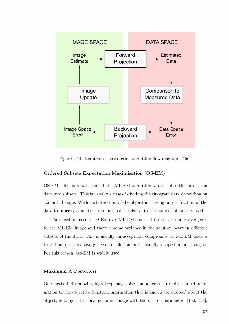
IMAGE SPACE DATA SPACE
Image SpaceError
ForwardProjection
BackwardProjection
ImageUpdate
Comparison toMeasured Data
Data SpaceError
ImageEstimate
EstimatedData
Figure 2.14: Iterative reconstruction algorithm flow diagram. [150].
Ordered Subsets Expectation Maximisation (OS-EM)
OS-EM [151] is a variation of the ML-EM algorithm which splits the projection
data into subsets. This is usually a case of dividing the sinogram data depending on
azimuthal angle. With each iteration of the algorithm having only a fraction of the
data to process, a solution is found faster, relative to the number of subsets used.
The speed increase of OS-EM over ML-EM comes at the cost of non-convergence
to the ML-EM image and there is some variance in the solution between different
subsets of the data. This is usually an acceptable compromise as ML-EM takes a
long time to reach convergence on a solution and is usually stopped before doing so.
For this reason, OS-EM is widely used.
Maximum A Posteriori
One method of removing high frequency noise components is to add a priori infor-
mation to the objective function; information that is known (or desired) about the
object, guiding it to converge to an image with the desired parameters [152, 153].
57
This is similar to implementing a penalty term in each iteration, to influence the
smoothness or edges of the images. Anatomical information from hybrid PET/MRI
or PET/CT may also be used to guide the structure of the image [154, 155], which
overcomes a loss in spatial resolution. These methods add a lot of complexity to the
reconstruction and are often unused in the clinical environment due to the difficulty
in choosing the correct parameters.
2.5.9 Image Reconstruction Software
STIR
The Software for Tomographic Image Reconstruction (STIR) library [156] is an open
source software (written in C++), focused on 3D PET iterative image reconstruc-
tion, though 3D analytic algorithms are also supported. The software has been
made available since 2000, originating from the PARAPET project and is some of
the most widely used reconstruction software within the field. STIR includes li-
braries for image and projection data manipulation, file format conversions as well
as the algorithms for reconstruction. Both sinograms and list mode data are sup-
ported. The current stable version of the library is v3.0.
CASToR
Customizable and Advanced Software for Tomographic Reconstruction (CASToR)
[157] is a much more recent software package (written in C++) for iterative image
reconstruction with PET, SPECT and CT. Includes tools for general image pro-
cessing and data processing, including a conversion of ROOT data to the CASToR
format. Analytical algorithms are not yet implemented. The current stable version
is v2.1.
MIRT
The Michigan Image Reconstruction Toolbox (MIRT) [158] is a collection of open
source algorithms written in Mathwork’s MATLAB language. Included are a number
of iterative and analytic algorithms for PET, SPECT, x-ray, CT and MRI.
58

2.6 Conclusion
This chapter presents an overview of PET operation and the many areas of active
research within the field. Of particular interest are the different approaches to
improve sensitivity, spatial resolution and signal-to-noise ratio of the image. The
first route is to employ faster scintillation materials and photodetectors to improve
the timing resolution, the second is to improve the geometrical coverage of the
scanner - both of these likely require an increase in the cost of componentry.
A potential solution is to use lower cost nanocomposite or transparent ceramic
scintillation materials, to shape a scanner which is geometrically efficient; a mono-
lithic continuous cylindrical shell architecture. Silicon photomultipliers seem the
obvious choice for coupling to the shell; they are physically small enough to be used
both outside and inside the ring and have superior detection capabilities compared
to PMTs or APDs (mass production should also see an improvement in cost).
This geometry leads to several important design questions. For an optically
translucent material, what is the optimum thickness at which to make the shell? It
is assumed that detections may be lost if the scattering is too great. There are also
many different materials available - which of these has the superior performance for
this application? Before reaching full image reconstruction, methods for determining
coincidence detection and generating lines of response must also be explored.
59

Chapter 3
Monolithic Nanocomposite and
Transparent Ceramic Scintillation
Detectors for use in Positron
Emission Tomography
3.1 Introduction
Detection and characterisation of high-energy photons is an inherently challenging
task due to their highly penetrating nature. Semiconductor detectors are unable to
directly detect such photons with high efficiency, due to the limited detector thick-
ness, low density and low effective atomic number of most semiconductor materials
[32]. To increase the probability of detecting high energy photons, in most appli-
cations it is necessary to optically couple an optical photodetector to a scintillator.
When a high-energy photon interacts with a scintillator, the energy deposited is
absorbed by atoms in the scintillator (commonly cerium, europium or thallium) and
re-radiated as multiple lower-energy photons, typically in the optical range, which
are easily detected by the photodetector. Many scintillator materials now exist,
including some with very high stopping power due to their very high density and
effective atomic number. The best of these also provide high light output, high
energy resolution and fast decay time, and emit wavelengths which are well-suited
to detection by solid-state silicon detectors or photomultiplier tubes.
60

Good scintillator materials are nearly transparent at the emission wavelength,
and so can be made as thick as desired to achieve the required detection probability.
The overwhelming majority of high-performance scintillator materials in use today
are inorganic crystals, which offer high stopping power and good light output at
wavelengths compatible with solid-state detectors and photomultiplier tubes. While
they offer many excellent scintillation properties, crystal scintillators are intrinsi-
cally challenging to manufacture, requiring lengthy growth periods at very high and
carefully regulated temperatures [26, 27]. Although some materials can be grown
to quite large crystal sizes, they are generally brittle and difficult to cut or machine
to anything other than relatively simple shapes (such as polyhedral blocks or occa-
sionally cylinders); some materials which have many good optical and scintillation
properties are also hygroscopic, requiring careful protection of the crystal to avoid
degradation.
For applications requiring position sensitivity, the dominant approach is to op-
tically couple discrete scintillator crystals to individual photodetector pixels in an
optical photodetector array to form a detector block. Naturally, the most common
crystal shape for this application is a rectangular prism. High-resolution and long
axial field of view PET systems may utilise many tens of thousands of such crystals;
if the scanner is capable of discerning depth of interaction, these crystals may be
present in multiple layers. In a discrete-crystal PET system, each crystal is normally
optically isolated from the others, and covered with a reflective coating on five of
its six sides. Assembling the arrays needed for a large PET system rapidly becomes
more difficult as the crystal size decreases and the scanner dimensions increase, with
the scintillator arrays representing a substantial fraction of the cost of the scanner
[5, 6, 4]. Furthermore, since a cylindrical shell cannot be divided into a finite number
of equal-sized rectangular prisms without introducing gaps, sensitivity varies with
respect to the angle of rotation around the central axis. This problem is even worse
for PET systems which are intended to have a spherical or D-shaped geometry.
For PET, an alternative to arrays of discrete scintillator crystals is for each de-
tector block to use a monolithic slab of scintillator material coupled to a pixellated
photodetector array. The distribution of optical photons arriving at the detector can
then be used to estimate the point of interaction within the crystal. This signifi-
61

cantly complicates the task of coincidence detection, but offers the major advantage
of simplified manufacturing compared to the discrete-crystal model. Monolithic
scintillators are normally fabricated as rectangular prisms. However, growing large
crystals of uniformly high quality remains technically challenging, and the materials
are still not easily fabricated into non-rectangular shapes.
Two new classes of materials have recently emerged as lower-cost alternatives
to single-crystal scintillators, particularly where complex shaping of the scintillator
is required: nanocomposites [102] and transparent ceramics [159]. Nanocomposites
are a uniform mixture of inorganic scintillator nanocrystals and a polymer binder
or matrix, which itself may also be a scintillating material. Although the nanocom-
posite has a lower density and effective atomic number (and hence stopping power)
compared to the single-crystal solid form of its inorganic scintillator component,
these parameters are still significantly higher than those of pure polymer scintillator
materials. Other important parameters, such as optical photon yield and wave-
length, are also similar (but not identical) to those of the bulk material. On the
other hand, transparent ceramic/garnet scintillators are chemically related to exist-
ing single-crystal scintillator materials, but with a polycrystalline structure. Many
of the desirable properties of comparable single-crystal scintillators are retained (in
particular, high stopping power and light output), however, they can be fabricated
more rapidly at much lower temperatures, and formed into complex shapes much
more easily than monocrystalline scintillator materials.
A common shortcoming of both nanocomposites and transparent ceramic scin-
tillators is their lower optical transparency compared to single-crystal scintillators.
In the case of nanocomposites, the difference between the refractive indices of the
nanocrystal scintillator and the matrix polymer leads to Rayleigh scattering and
reduced transmittivity. A similar problem also exists to some extent in ceramic
garnet scintillators due to the presence of grain boundaries in the material. Slabs of
single-crystal scintillator material can be made as thick as necessary to achieve the
desired sensitivity, due to the low optical attenuation of the material. However, this
is not the case for either nanocomposites or ceramics, as beyond a certain optimal
thickness, scattering and attenuation degrade the optical signal to the point where
it is no longer useful in providing an accurate estimate of the point of interaction
62

within the scintillator. Therefore, determining the optimal thickness for the scin-
tillator is an important design question for those wishing to utilise these materials
in PET systems and other radiation detection applications. In this context, opti-
mal refers to that thickness which maximises the number of photons whose point
of interaction can be estimated within a specified threshold of accuracy. Too thin,
and the probability of detection will be too low; too thick and many of the optical
photons may be absorbed before reaching the optical photodetector, resulting in an
inaccurate position estimation.
This work proposes a general method for determining optimal thickness of a
monolithic scintillator slab, given the physical properties of the scintillator mate-
rial, based on cubic spline interpolation between results obtained from a set of
Monte Carlo simulations. The method is demonstrated by applying it to provide
a quantitative comparison between a range of promising nanocomposite and trans-
parent ceramic scintillators. Section 3.2 discusses the specific methods to be used in
this work and introduces the proposed thickness-optimisation technique; Section 3.3
presents results comparing scintillator performance with two fixed thicknesses plus
the optimal thickness for each material, and discusses the key implications. Finally,
the outcomes of this research are summarised in Section 3.4.
3.2 Materials and Methods
In this section, a Monte Carlo-based approach to the optimisation of monolithic scin-
tillator slab thickness for a given material is described. The method is applicable to
any material with accurately characterised physical and optical properties. Simu-
lations are performed using version 8.0 of the Geant4 Application for Tomographic
Emission (GATE), which extends the well-known Geant4 Monte Carlo framework
to enable complex simulations of the interaction of radiation and matter to be con-
structed via text-based descriptions of geometry and materials [160, 161, 162].
3.2.1 Performance Metric and Optimisation Algorithm
In scintillator-based imaging systems such as PET, the probability of detecting an
emitted photon is limited by thickness of the scintillator and the radiation length in
63

the scintillator material at the wavelength (or wavelengths) of interest. For imaging
systems based on monolithic scintillators, detection probability must be defined
more specifically, also taking into account the accuracy of detection - that is, the
probability that the location of a the first energy-depositing interaction within the
scintillator can be estimated to within a certain tolerance of the true location inside
the scintillator. Using this metric, “optimal thickness” of a large rectangular slab of
scintillator material may be defined as the thickness which enables the greatest
fraction of incident photons to be localised to within a specified distance
of the true point of interaction. It is reasonable to expect that such an optimum
exists; if the scintillator is too thin, detection efficiency will be very low due to the
small number of primary photons which will interact with it (although they can
be localised very precisely within the slab), while if it is too thick, the optical
attenuation of the scintillator will cause too many of the scintillation photons to be
absorbed for accurate determination of the point of interaction, and the probability
of multiple Compton scatter events (which manifest as a multi-point emission within
the scintillator) increases.
To determine the optimal monolithic scintillator thickness for each material, for
a given gamma photon energy, a series of GATE simulations of a given scintillator
material are performed with different slab thicknesses. An exhaustive evaluation
may be performed for a range of potential thicknesses; however, for most materials
this is not necessary. The optimal thickness may be determined by the following
procedure:
1. Choosing the desired threshold of detection accuracy suitable for the proposed
application;
2. Simulating photon interactions with the scintillator with a small number of
thicknesses;
3. Applying the chosen location-determination algorithm to the observed optical
photon maps on both sides of the scintillator;
4. Determining the probability of being able to estimate the first point of inter-
action of the incident gamma photons to within the chosen threshold for each
simulation; and
64

5. Apply cubic spline interpolation between the measured points and determine
its maximum from the first derivative.
This approach will work with any position estimation algorithm, such as several
of those described in Section 2.4. In this work, we utilise an error-minimisation
method to fit the location and emission intensity parameters of a simple analytic
model to the observed patterns of photon emission on both the front and back side
of the scintillator.
3.2.2 Simulation Parameters
To evaluate the chosen performance metric and develop a model for its optimisation,
a series of GATE simulations were performed, using the basic geometry in Figure
3.1. The depth of the scintillator slab (in the z dimension - for a PET scanner,
this would be the radial dimension) was varied - between 5 mm and 35 mm in
steps of 5 mm for the transparent ceramics, and between 10 mm and 70 mm in
steps of 10 mm for the nanocomposites. Each simulation consisted of 20000 primary
photons.
3.2.3 Detector Geometry
The geometrical design of the scintillation detector (3.1) is very similar to the
monolithic detector model previously described in [163] and simulated in Geant4
and GATE [164]. In this study, the scintillator volume of width×height×depth =
20 mm×20 mm×t; Figure 3.1 shows an example where t = 10 mm.
The detectors are arranged in a double-sided readout (DSR) configuration, a
design which supports accurate localisation of the point of interaction over a wider
range of scintillator thicknesses compared to either front-only or back-only readout
systems [62]. This is particularly important for the lower density nanocomposite
materials discussed here. The detectors themselves are modelled as a simple silicon
photodiode; the pixellated detector planes are coupled to the scintillator via thin
layers of Meltmount and epoxy (0.05 mm and 0.1 mm respectively), while the exte-
rior surface is covered by a 1 mm polymer/metal layer representing the electronics
in the detector. Non-detector faces of the scintillator are covered with non-reflective
65

(a) (b)
Figure 3.1: A single photoelectric interaction, captured using a dual photodetector
configuration with a 10 mm thick GYGAG:Ce scintillator slab. The incoming γ
photon (red) interacts with the scintillator (blue) and emits a shower of 550 nm
optical photons (shown in green). Note that the only a small fraction of the optical
photon paths are shown for clarity. Subfigures (a) and (b) provide two different
views of the same interaction.
black paint. Detector pixels are 1 mm×1 mm (with zero assumed dead space).
3.2.4 GATE Parameters
The following parameters were used with GATE version 8.0 and Geant4 version
10.2.2.
System
A GATE optical system is implemented for accurate optical tracking of the scin-
tillation photons and modelling the relevant physics, including optical attenuation,
scattering and surface properties.
Physics
GATE uses the Geant4 low background experiment (LBE) physics list, as it is recom-
mended for simulations incorporating optical photon transportation and scintillation
processes [165]. Compton scattering and photoelectric processes have been added
66

for gamma photon interactions, along with all processes relating to optical interac-
tions, including bulk absorption, Rayleigh scattering, Mie scattering and boundary
processes.
Surface Properties
The UNIFIED model was used to define the optical surface properties of the in-
terfaces between materials. To simulate the absorptive black paint covering the
scintillator material, the ground-front-painted finish was used; the reflectivity is set
to zero so that optical photons are not internally reflected. The optical roughness of
surfaces can be specified by altering the σα value (defined as the standard deviation
of the Gaussian distribution of micro-facets around the average surface normal);
however, it has previously been shown that for the scintillator-Meltmount-detector
interfaces, this parameter has a minimal influence on the accuracy of estimation of
the point of interaction due to the large size of detector pixels relative to the micro-
facets [62, 166]. Therefore, this parameter has been set to σα = 0.1 (corresponding
to a polished surface). The interface between the detector and the Meltmount layer
has been specified as perfect-apd, which assumes perfect flatness and 100% efficiency.
Source
The source is a simple monochromatic 511 keV photon gun. Since the focus of this
work is providing a mechanism to compare optimal thicknesses of different scintilla-
tor materials, rather than the localisation algorithm itself, all photons are directed
at the centre of the scintillator slab, parallel to the z axis. For optimal thickness
determination, 20000 primary (γ) photons have been fired at the detector for each
evaluated combination of scintillator thickness and material. For determination of
spatial error and analysis of scatter composition, 200000 primary (γ) photons were
used.
3.2.5 Nanocomposite Loading
Figure 2.10(a) and 2.10(b) demonstrate that for nanocomposite materials, optical
transmittivity and stopping power are both strongly influenced by the scintillator
loading fraction; however, the effects are in opposition to one another. Higher
67

loading (i.e. a higher fraction of nanoscintillator compared to the matrix material)
results in a higher average density and effective atomic number (and hence stopping
power); however, optical attenuation is increased, limiting the benefits of a high
loading factor since many of the scintillation photons are scattered and/or absorbed
before they can be detected.
To ensure that enough scintillation photons can be detected for an accurate esti-
mate of the point of interaction to be determined, a reasonable approach to choosing
an appropriate loading factor is to balance the optical attenuation length equally
against the gamma radiation attenuation length. If a DSR detector configuration is
being used with this approach, the thickness of the scintillator which satisfies this
criterion is doubled compared to a single-sided readout design (i.e. for DRS, the
maximum distance away from any detector is only half of the scintillator thickness).
The scintillator loading volume fraction may be found by considering Figure 2.10(a).
For example, a 2 cm thick nanocomposite detector made from LaF3:Ce nanoscin-
tillator material in an oleic acid matrix (with double-sided readout) would require
a 1 cm optical attenuation length (half the length of the scintillator) to satisfy the
condition. A 1 cm attenuation length for LaF3:Ce is equal to approximately 17%
scintillator loading by volume.
Alternatively, if a specific attenuation length is required - for example, 50% at-
tenuation of 511 keV gamma photons (the half value layer or HVL) - then a suitable
loading factor and thickness can be computed such that the gamma radiation at-
tenuation length equals the optical attenuation length. In the case of a single-sided
detector, the point of intersection of the curves in Figure 2.10(a) and 2.10(b) can
be found; for the DSR configuration, the optical attenuation length only needs to
be equal to half of the HVL. This may be more easily seen in figure 3.2, which
shows both of these plots overlaid for LaF3:Ce OA. The scintillator volume fraction
satisfying the condition in this case is ∼5%, at the point of intersection. All of the
loading factors used in the simulations are shown in Table 3.1.
3.2.6 Scintillation Event Position Determination
Estimation of the most likely coordinates of the first point of interaction for each
(interacting) primary event is performed in Matlab through analysis of the “Hits”
68

Figure 3.2: Overlaid plots of optical attenuation and HVL / 2 for LaF3:Ce oleic
acid. The point of intersection between these curves is used to determine appro-
priate scintillator loading factor for the nanocomposite; in this case, the point of
intersection occurs at ∼5%.
Nanoparticle LaBr3:Ce Gd2O3 LaF3:Ce LaF3:Ce YAG:Ce
Matrix PS PVT OA PS PS
1 cm load (%) 19 4.6 34 50 50
2 cm Load (%) 9 4.6 17 50 50
HVL Load (%) 3 4.6 5 50 28
T. Opt. (%) 7 4.6 12 50 37
Table 3.1: A summary of the loading factors by % volume, used in these simulations.
Calculated as described, using figures 2.10(a) and 2.10(b). The loading factor for
optimal thickness (denoted T. Opt.) was chosen based on a 3 cm thick slab, using
the same methodology.
69

(a) Detected photons (front)
(b) Detected photons (back)
Figure 3.3: An analytic model of the expected photon map is jointly fitted to the
photon distributions observed on both the front and back of the scintillator. The
calculated parameters for the function are then used to estimate the position of
interaction of the initial gamma photon and the number of scintillation photons
emitted.
70

(c) Fitted model (front)
(d) Fitted model (back)
Figure 3.3: (Continued from previous page). The optical photon distribution on the
front and back detector and shown in Figure 3.3(a) and 3.3(b) respectively, while
Figure 3.3(c) and 3.3(d) show the analytic functions fitted to these distributions
using (3.1) and (3.2).
71

γ photon
Jb(xd, yd, 0)
J0(xs, ys, zs)T
Jf(xd, yd, T )
z
xy
Figure 3.4: The incident γ photon strikes the scintillator slab at point (xs, ys, zs),
with intensity J0. The optical photon intensity detected on pixels (of dimensions
∆x×∆y) at position (xd, yd) on the back and front faces of the detector are given
by Jb (3.1) and Jf (3.2) respectively.
list-mode data recorded during the simulation. This file records the location of
all photon interactions with the scintillator and detector (both gamma and optical
photons). The true 3D points of interaction with the scintillator, as well as the
number of photoelectric, Compton and Rayleigh scatter events which occur inside
the scintillator material for each interacting primary (γ) photon are logged, together
the 3D coordinates at which any scintillation photons interact with the detector
surface. The time of each interaction and deposited energy are also logged. An
example of the detected photon distributions is shown in Figure 3.3(a) and 3.3(b).
Detected optical photons are isolated into those associated with an individual
primary via a timing window (chosen to suit the time constants of each scintillator
material). The optical photon distributions on the surface of each detector are
binned into 1 mm×1 mm pixels.
A parametric model of the predicted photon distribution (as a function of lo-
cation within the scintillator slab) is derived from (2.8), and fitted to the discrete
photon map via the Levenberg-Marquardt minimisation algorithm. The geometry
is described in Figure 3.4. For a scintillation event occurring at position (xs, ys, zs),
the number of photons arriving at a pixel of dimensions (∆x×∆y) located at (xd, yd)
72

on the back face is given by:
Jb(x, y) =J0zp∆x∆ye−
√(xs−xd)2+(ys−yd)2+z
2s
λ
4π ((xs − xd)2 + (ys − yd)2 + z2s)
32
(3.1)
where J0 is the number of emitted scintillation photons, and λ is the radiation
attenuation length. Similarly, on the front face (i.e. the first face through which
the incident photon passes), the expected number of photons arriving at the same
pixels is given by:
Jf (x, y) =J0(T − zp)∆x∆ye−
√(xs−xd)2+(ys−yd)2+(T−zs)2
λ
4π ((xs − xd)2 + (ys − yd)2 + (T − zs)2)32
(3.2)
where T is the thickness of the scintillator slab.
To account for total internal reflection within the scintillator slab, Jb is set to
zero anywhere outside a circle of radius
Rb = zsnmm
n2s − n2
mm
(3.3)
where nmm is the refractive index of Meltmount (the optical coupling compound)
and ns is the scintillator’s refractive index. Similarly Jf is set to zero outside of a
circle of radius
Rf = (T − zs)nmm
n2s − n2
mm
(3.4)
An example of the fitted analytic model is shown in Figure 3.3(c) and 3.3(d).
3.2.7 Materials
Scintillator properties were taken from the literature where possible (see Table 2.4
and 2.5) or, for the case of the nanocomposites, calculated via the methods described
in Section 2.4 (see (2.11) and (2.12)). Several of the optical and physical properties,
including the density, refractive index and optical absorption length are dependent
upon the loading factor of the nanoscintillator relative to the binder. The scintil-
lation spectrum is assumed to be monochromatic at the peak emission wavelength,
so refractive index and absorption length are single values (calculated for the peak
wavelength).
The silicon and epoxy layers use the default parameters found in the GATE ma-
terial database, while Meltmount has been created using the chemical composition
described by Van der Laan et al. [164].
73

As a reference material, equivalent simulations were also conducted using Lu2SiO5
(LSO), which is a well known scintillation material, common in many PET systems.
3.3 Results and Discussion
3.3.1 Calculation of the Optimal Scintillator Thickness
The relationship between scintillator thickness and the number of events detected is
shown in Figure 3.5 and 3.6 for the nanocomposite and transparent ceramic scintilla-
tors, respectively. These plots include separate curves for detections whose estimated
point of interaction has been correctly detected within spatial error limits of 1 mm,
2 mm, 3 mm, 4 mm, 5 mm and all detections regardless of accuracy; ∆D is the total
spatial error (∆D =√
∆x2 + ∆y2 + ∆z2). The location of the maxima of each of
these curves is summarised in Table 3.2.
Of the nanocomposite materials evaluated, LaF3:Ce-polystyrene offers the max-
imum probability of detection for ∆D ≥ 3 mm, and is only slightly worse than
YAG:Ce-PS at ∆D ≤ 2 mm; in all cases, this sensitivity is achieved by LaF3:Ce-
polystyrene with a much thinner slab of scintillator than for the other materials.
This is chiefly due to the high loading factor (and hence high density and Zeff ) rel-
ative to the other nanocomposite materials. As previously discussed, however, the
loading factor cannot be increased without compromising the transmittivity of the
nanocomposite. YAG:Ce-polystyrene offers a fair compromise between sensitivity
and accuracy of interaction localisation. It has the highest probability of detection
(of the nanocomposites) for ∆D ≤ 1 mm and ∆D ≤ 2 mm and offers sensitivity
which is comparable to LaF3:Ce-PS for ∆D ≤ 3 mm.
With their high density and Zeff , the transparent ceramics offer a much higher
probability of detection at any given slab thickness compared to the nanocomposite
materials. As with the nanocomposites, the key differences between the different
ceramic materials related to detection efficiency and accuracy of position estimation
are their emission wavelengths and their optical transmittivity. GAGG:Ce, GLu-
GAG:Ce and LuAG:Pr all have similar attenuation coefficients at 511 keV, however
GYGAG:Ce has by far the highest optical transmittivity, allowing a higher pro-
portion of the the scintillation photons to reach the detectors. While GYGAG:Ce
74

achieves the highest overall probability of detection, the thickness required for this
to occur is ≥45 mm and a high proportion of events are localised with an error
∆D > 5 mm. As for the nanocomposites, a higher scintillator thickness increases
the impact of coherent optical photon scattering, making it increasingly difficult for
the localisation algorithm to accurately estimate the point of interaction. The ben-
efits of high optical transparency are therefore limited if density and Zeff are such
that a very thick slab of scintillator is required, since although a large fraction of
photons will be detected, their point of interaction cannot be accurately localised.
GLuGAG:Ce provides the highest probability of detection for all finite ∆D lim-
its. This is the most dense material while being marginally more transparent than
GAGG:Ce and LuAG:Pr. If the scanner is to be optimised for accuracy rather than
sensitivity, an optimal thickness for GLuGAG:Ce would be approximately 20 mm,
yielding detection of about 46% of photons to within 1 mm of their true point of
interaction, and 62.5% of photons within 5 mm. On the other hand, increasing the
scintillator thickness to around 27.5 mm will increase the latter figure of merit to
67.5% while reducing the former to around 43% - demonstrating that further in-
creases in scintillator thickness will capture more photons, but with progressively
decreasing accuracy. The maximum sensitivity of GAGG:Ce and LuAG:Pr are some-
what lower, peaking at around 48% and 60% of incident photons, respectively (for
events localised to within 5 mm of the true location).
In summary, while all transparent ceramic scintillator materials significantly out-
perform the evaluated nanocomposite materials, there may be price points at which
certain nanocomposite materials offer sufficient performance to justify their use in
a PET scanner design.
3.3.2 Analysis of Photoelectric vs Compton Interactions
The probability of photoelectric, single and multiple Compton interactions in each
scintillator type is shown in Tables 3.3, 3.4, 3.5 and 3.6 for 1 cm, 2 cm, half-value
layer thickness and optimal thickness monolithic slabs. LSO has been used as a
benchmark scintillator for comparison with these materials, as may be seen in Tables
3.3, 3.4 and 3.5, which show the percentage and composition of events detected for
scintillators of 1 cm, 2 cm and the HVL of each material, respectively.
75

(a) Gd2O3 PVT (4.6 % loading)
(b) LaBr3:Ce PS (7 % loading)
Figure 3.5: Percentage of events detected to a specified accuracy of 1 mm, 2 mm,
3 mm, 4 mm, 5 mm and all detections as a function of scintillator thicknesses for
nanocomposite materials. Median values with interquartile ranges are shown.
76
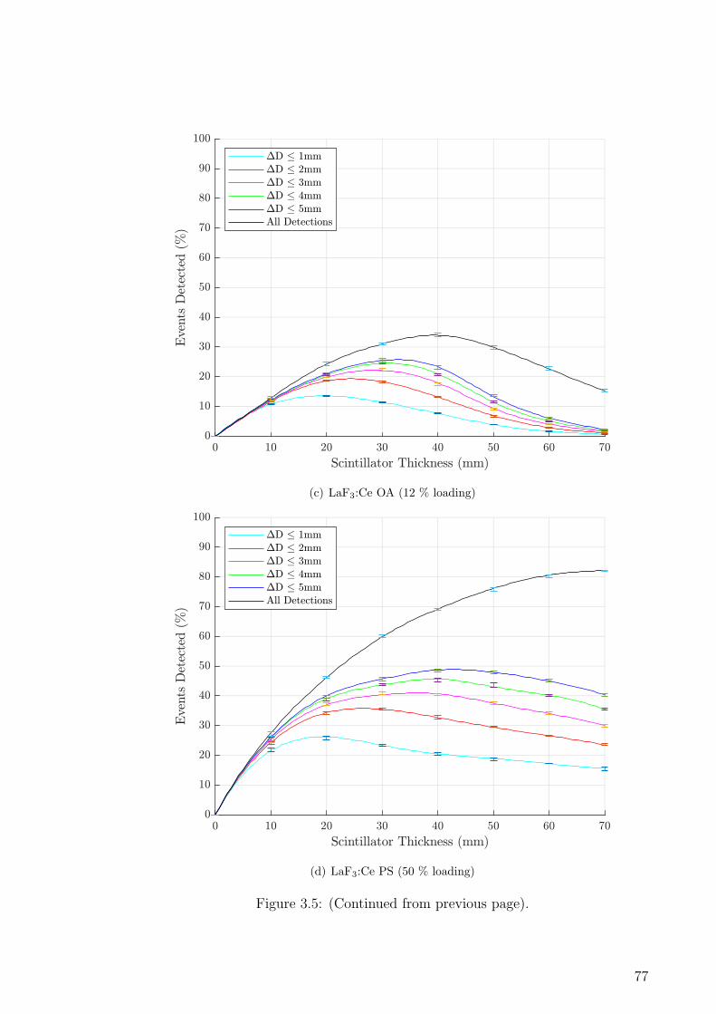
(c) LaF3:Ce OA (12 % loading)
(d) LaF3:Ce PS (50 % loading)
Figure 3.5: (Continued from previous page).
77

(e) YAG:Ce PS (37 % loading)
Figure 3.5: (Continued from previous page).
Scintillator
∆D ≤ 1 mm ∆D ≤ 2 mm ∆D ≤ 3 mm ∆D ≤ 4 mm ∆D ≤ 5 mm All Detections
T. Opt.(mm)
P. D.(%)
T. Opt.(mm)
P. D.(%)
T. Opt.(mm)
P. D.(%)
T. Opt.(mm)
P. D.(%)
T. Opt.(mm)
P. D.(%)
T. Opt.(mm)
P. D.(%)
Gd2O3 PVT 32.91 19.84 48.18 27.93 52.71 32.52 57.18 35.15 62.61 37.21 - -
LaBr3:Ce PS 34.56 23.02 44.13 28.88 49.33 32.67 51.61 35.36 53.78 36.70 61.33 45.45
LaF3:Ce OA 19.58 13.58 24.26 19.33 28.50 22.15 30.78 24.58 32.66 25.73 39.42 33.97
LaF3:Ce PS 19.21 26.23 26.61 35.73 36.35 40.95 39.41 45.66 42.60 48.83 - -
YAG:Ce PS 27.91 27.72 37.12 36.28 41.13 40.43 44.61 43.76 46.79 45.63 52.43 58.69
GAGG:Ce 12.58 37.17 13.57 42.66 13.85 45.04 13.91 46.73 13.98 47.95 14.53 54.46
GLuGAG:Ce 19.25 46.33 25.25 56.48 26.70 62.37 27.39 65.71 27.54 67.82 28.08 79.94
GYGAG:Ce 29.78 44.13 31.13 52.78 40.54 59.09 41.68 63.67 42.63 66.75 - -
LuAG:Pr 15.69 42.28 18.31 51.26 18.78 55.50 18.81 58.08 18.96 59.95 19.52 69.09
Table 3.2: Optimum scintillator thickness (denoted T. Opt.) and corresponding
probability of detection (P. D.) within a limit of 1, 2, 3, 4, 5 and all detections.
∆D is the total error in position estimation for the point of interaction, for both
nanocomposite and transparent ceramic scintillator materials.
78

(a) GAGG:Ce
(b) GLuGAG:Ce
Figure 3.6: Percentage of events detected to a specified accuracy of 1 mm, 2 mm,
3 mm, 4 mm, 5 mm and all detections as a function of scintillator thicknesses for
transparent ceramic materials. Median values with interquartile ranges are shown.
79

(c) GYGAG:Ce
(d) LuAG:Pr
Figure 3.6: (Continued from previous page). Note that the x-axis is slightly longer
for GYGAG.
80

The analytic function used for estimating the location of the point of interaction
assumes that all interactions are photoelectric. In reality, many interactions involve
one or more Compton (incoherent) scatter events, which potentially results in more
than one point of energy deposition within the scintillator slab. Since energy is lost in
each Compton interaction, the probability of photoelectric absorption increases with
each subsequent scatter. The result is a more spread-out (and, in general, irregular)
projection of optical photons on the detector surface following a multi-interaction
event compared to a simple photoelectric interaction or a Compton interaction where
the scattered photon does not undergo any further interaction with the scintillator.
The cross-sections determining the probability of interaction via photoelectric
absorption and Compton scattering are complex functions of the electronic structure
of the atoms in the photon path. Photoelectric absorption cross-section is approxi-
mately proportional to the 4th or 5th power of Zeff and proportional to the 3.5th
power of wavelength. By contrast, Compton cross-section is approximately propor-
tional to the density of the material and wavelength. At 511 keV, the dominant
process is Compton scattering for both nanocomposite and ceramic scintillators,
although a substantial minority of photons are absorbed photoelectrically in both
cases (much more so for the ceramics). The majority of cases for the evaluated
scintillator materials listed in Tables 3.3-3.6 involve either purely photoelectric in-
teractions, single or double Compton scatter events (more heavily weighted towards
photoelectric and single-Compton events in the case of the ceramic materials).
The high loading factor of LaF3:Ce-PS makes it the best-performing nanocom-
posite in terms of the proportion of photoelectric interactions. All of the transparent
ceramic materials offer performance which is much more similar to the benchmark
performance of the LSO than even the LaF3:Ce-PS nanocomposite, both in terms
of the total proportion of events detected and the percentage of these interactions
which are photoelectric. In terms of scattering composition, LuAG:Pr has char-
acteristics most similar to the LSO with only ∼4% difference in the number of
photoelectric interactions recorded, though GLuGAG:Ce and GAGG:Ce still have
respectable numbers (∼10% and 13% difference respectively). GYGAG:Ce has less
then half the photoelectric count of LSO, again due to a lower density. Interest-
ingly, LuAG:Pr has the highest percentage of events detected at 1 cm scintillator
81

thickness, but as this is increased to 2 cm all other ceramics have a higher rate of
increase (with GLuGAG:Ce increasing the most).
Multi-interaction events degrade the accuracy of the fitting algorithm, which
assumes all energy is deposited at a single location. Fortunately, since the fraction
of photon energy deposited is related to the angle of scatter, the magnitude of this
degradation is smaller than at first may appear. If the first interaction deposits
a large fraction of the gamma photon’s energy, the angle of scatter will also be
large - but the reduction in photon energy reduces the mean free path length of
the scattered photon compared to the initial 511 keV gamma photon. Therefore,
the resulting optical photon distribution will be dominated by the first point of
interaction, with only a minor impact on the position of the endpoint of the line
of response. If the amount of energy deposited at the first point of interaction is
small, the angle of scatter will also be small. Therefore, subsequent interactions will
follow a trajectory through the scintillator which is not very different to that of the
original photon. If the next interaction is photoelectric (which is now more likely as
the photon energy has been reduced), the resulting line of response will only deviate
slightly from the true line of response (and will be slightly pulled back towards the
true LOR by whatever energy was deposited at the first point of interaction). The
largest error introduced by such events will be in the radial direction (depth). The
intermediate case - an initial or secondary Compton scatter which deposits some
non-trivial amount of energy, followed by further multiple Compton interactions,
results in the largest errors in the placement of the line of response.
3.3.3 Spatial error
The mean and median errors in each dimension of the estimated positions of gamma
photon interactions (where the ground truth is defined as the first point of interac-
tion in the scintillator slab) together with their interquartile ranges (central 50% of
errors) and standard deviations are summarised in Tables 3.7-3.10, for scintillator
thicknesses of 1 cm, 2 cm, the HVL thickness and optimal thickness, respectively.
These results include all event types (both pure photoelectric events and events in-
cluding one or more Compton scatters). Monocrystalline LSO has again been used
as a benchmark scintillator for comparison with each of the materials.
82

ScintillatorPhotoelectric/Compton scatter composition Total events
detected (%)PE (%) C1 (%) C2 (%) C3 (%) C4 (%) C5+ (%)
Gd2O3 PVT 1.58 87.98 9.37 0.91 0.14 0.02 11.70
LaBr3:Ce PS 2.47 84.04 11.63 1.62 0.22 0.02 15.17
LaF3:Ce OA 6.55 76.00 14.46 2.51 0.41 0.07 20.81
LaF3:Ce PS 9.75 71.17 15.41 3.05 0.56 0.07 27.02
YAG:Ce PS 1.89 78.67 15.47 3.23 0.62 0.12 21.68
GAGG:Ce 26.95 53.13 15.73 3.51 0.57 0.11 45.12
GLuGAG:Ce 24.34 55.14 16.33 3.55 0.57 0.07 48.50
GYGAG:Ce 14.08 61.98 18.33 4.57 0.86 0.17 40.14
LuAG:Pr 30.09 52.47 14.16 2.84 0.39 0.04 49.79
LSO 34.85 49.36 13.11 2.34 0.31 0.03 55.57
Table 3.3: Distribution of photoelectric and Compton-scattered interactions for a
1 cm thick scintillator slab, expressed as the percentage of events of this type which
are detected out of the total number of primary photons incident on the detector.
CN denotes N Compton scatter interactions prior to either final photoelectric ab-
sorption or escape from the scintillator. Monocrystalline LSO is also included as a
reference benchmark.
ScintillatorPhotoelectric/Compton scatter composition Total events
detected (%)PE (%) C1 (%) C2 (%) C3 (%) C4 (%) C5+ (%)
Gd2O3 PVT 1.34 83.90 12.56 1.90 0.22 0.07 21.29
LaBr3:Ce PS 1.11 83.99 12.72 1.84 0.28 0.06 22.08
LaF3:Ce OA 3.32 77.77 15.57 2.76 0.49 0.10 26.09
LaF3:Ce PS 9.84 64.15 19.87 4.96 0.95 0.23 45.09
YAG:Ce PS 1.86 71.85 19.76 4.95 1.21 0.37 37.82
GAGG:Ce 30.41 41.14 20.79 6.15 1.28 0.23 41.18
GLuGAG:Ce 24.33 49.12 19.88 5.39 1.06 0.21 71.59
GYGAG:Ce 14.14 54.38 22.75 6.84 1.56 0.34 62.65
LuAG:Pr 31.20 45.98 17.76 4.18 0.77 0.10 67.50
LSO 34.86 45.00 15.95 3.53 0.58 0.08 78.85
Table 3.4: Distribution of photoelectric and Compton-scattered interactions for a
2 cm thick scintillator slab.
83

ScintillatorPhotoelectric/Compton scatter composition Total events
detected (%)Thickness
HVL (mm)PE (%) C1 (%) C2 (%) C3 (%) C4 (%) C5+ (%)
Gd2O3 PVT 0.92 77.69 17.49 3.19 0.60 0.12 39.56 53.10
LaBr3:Ce PS 0.14 79.93 16.77 2.65 0.43 0.08 40.30 64.40
LaF3:Ce OA 0.28 81.42 15.45 2.47 0.33 0.05 26.92 64.90
LaF3:Ce PS 10.06 63.76 19.99 4.98 1.01 0.21 46.25 21.20
YAG:Ce PS 1.11 71.55 20.98 4.92 1.10 0.33 43.26 39.50
GAGG:Ce 26.91 53.04 15.80 3.52 0.64 0.08 46.64 10.60
GLuGAG:Ce 24.34 55.14 16.33 3.55 0.57 0.07 48.50 10.00
GYGAG:Ce 14.39 58.90 20.06 5.30 1.11 0.24 48.52 13.10
LuAG:Pr 30.13 52.73 14.02 2.74 0.34 0.04 47.30 9.29
LSO 35.14 50.59 12.04 1.96 0.26 0.02 48.10 7.99
Table 3.5: Distribution of photoelectric and Compton-scattered interactions for a
scintillator thickness equal to the half value layer for each scintillator material.
ScintillatorPhotoelectric/Compton scatter composition Total events
detected (%)Thickness
Opt. (mm)PE (%) C1 (%) C2 (%) C3 (%) C4 (%) C5+ (%)
Gd2O3 PVT 0.79 76.72 18.51 3.24 0.60 0.14 43.23 62.61
LaBr3:Ce PS 0.32 79.76 16.65 2.71 0.45 0.10 40.57 53.78
LaF3:Ce OA 1.20 79.75 15.83 2.64 0.48 0.09 30.84 32.66
LaF3:Ce PS 11.51 55.73 23.62 7.08 1.69 0.38 60.21 42.60
YAG:Ce PS 1.64 68.30 22.42 5.76 1.42 0.46 50.43 49.79
GAGG:Ce 22.17 52.64 19.34 4.81 0.90 0.14 53.03 13.98
GLuGAG:Ce 25.15 46.13 21.07 6.17 1.23 0.24 78.38 27.54
GYGAG:Ce 15.30 47.61 25.34 8.83 2.36 0.56 79.72 42.63
LuAG:Pr 31.61 46.25 17.24 4.08 0.71 0.11 67.61 18.96
Table 3.6: Distribution of photoelectric and Compton-scattered interactions for a
scintillator thickness equal to the optimal thickness for each scintillator material.
84

Scintillatorx error (mm) y error (mm) z error (mm) Total error (mm)
Med. Mean IQR SD Med. Mean IQR SD Med. Mean IQR SD Med. Mean IQR SD
Gd2O3 PVT 1× 10⁻⁵ 4× 10⁻³ 0.1 0.5 −3× 10⁻⁴ −3× 10⁻³ 0.1 0.5 −1× 10⁻¹ −6× 10⁻² 0.2 0.7 0.2 0.4 0.2 0.9
LaBr3:Ce PS −5× 10⁻⁴ −7× 10⁻⁴ 0.1 0.6 −3× 10⁻⁴ −3× 10⁻⁴ 0.1 0.6 −1× 10⁻¹ −4× 10⁻² 0.1 0.9 0.2 0.5 0.2 1.2
LaF3:Ce OA 1× 10⁻³ 3× 10⁻³ 0.3 1.0 −2× 10⁻³ −6× 10⁻⁴ 0.3 1.0 −1× 10⁻¹ 6× 10⁻² 0.4 1.3 0.5 1.0 0.6 1.6
LaF3:Ce PS −6× 10⁻⁴ −4× 10⁻³ 0.3 1.0 8× 10⁻⁴ 3× 10⁻³ 0.3 1.0 −1× 10⁻¹ 3× 10⁻² 0.3 1.2 0.4 0.9 0.5 1.6
YAG:Ce PS −4× 10⁻⁴ −6× 10⁻³ 0.1 0.6 4× 10⁻⁵ −2× 10⁻³ 0.1 0.6 −1× 10⁻¹ 6× 10⁻³ 0.4 1.0 0.3 0.6 0.3 1.2
GAGG:Ce 2× 10⁻⁵ −4× 10⁻³ 0.2 1.2 −3× 10⁻⁴ −2× 10⁻³ 0.2 1.2 −1× 10⁻¹ 1× 10⁻¹ 0.4 1.4 0.3 1.0 0.6 1.9
GLuGAG:Ce −2× 10⁻⁴ −2× 10⁻³ 0.1 1.1 −4× 10⁻⁴ 2× 10⁻³ 0.1 1.1 −1× 10⁻¹ 2× 10⁻¹ 0.4 1.4 0.3 1.0 0.6 1.8
GYGAG:Ce −7× 10⁻⁵ 1× 10⁻³ 0.1 1.1 −8× 10⁻⁵ 1× 10⁻³ 0.1 1.0 −1× 10⁻¹ 1× 10⁻¹ 0.3 1.3 0.3 0.9 0.5 1.8
LuAG:Pr 2× 10⁻⁵ 4× 10⁻³ 0.2 1.1 −5× 10⁻⁴ 4× 10⁻⁴ 0.2 1.1 −1× 10⁻¹ 2× 10⁻¹ 0.5 1.4 0.4 1.1 0.7 1.8
LSO −3× 10⁻⁴ −7× 10⁻³ 0.1 1.1 9× 10⁻⁵ 1× 10⁻³ 0.1 1.1 −1× 10⁻¹ 3× 10⁻¹ 0.4 1.4 0.3 1.0 0.7 1.8
Table 3.7: Mean and median errors in the estimation of the point of interaction
within a 1 cm thick scintillator slab, in each dimension and overall. Standard de-
viations and interquartile ranges (the spread of the middle 50% of errors) are also
listed.
The mean and median errors in each dimension are very small for all materials
at thicknesses of 1 and 2 cm, indicating that the localisation method introduces
minimal bias. The spread of error in x and y is smaller than the depth dimension,
with the difference becoming much more pronounced for thicker scintillator slabs
due to two factors: the increased probability of multiple interactions, and increased
Rayleigh scattering and attenuation prior to optical photon detection.
Figure 3.7 and 3.8 show a set of scatterplots showing position estimation dis-
tribution error in each dimension and in total as a function of depth for optimised
slabs of LaF3:Ce-PS and GLuGAG:Ce, respectively (Note that the threshold of
the colour scale is only approximately ∼10 % of the absolute maximum bin count,
to show greater detail in lower count bins). For these materials, the majority of
errors in each dimension are within < ±1 mm, with the majority of interactions oc-
curring within 5 mm of the detector surfaces. The outliers mostly corresponding to
multi-interaction events. The greatest lateral error (x and y) occurs around the half-
thickness of the scintillator slab, since this point is the furthest from either front or
back detector and therefore most susceptible to scatter and attenuation. The higher
density of the ceramic results in a larger fraction of events being detected close to
the front surface compared to the nanocomposite, resulting in an overall superior
performance for this material. These general observations also apply to the other
nanocomposite and ceramic scintillators.
85

(a) x
(b) y
Figure 3.7: Distributions of error in position estimation in each dimension as a func-
tion of depth for a LaF3:Ce-PS monolithic scintillation detector, at the calculated
optimal thickness. Figure 3.7(d) shows the distribution of total Euclidean error.
86

(c) z (depth)
(d) Total error
Figure 3.7: (Continued from previous page).
87

(a) x
(b) y
Figure 3.8: Distributions of error in position estimation in each dimension as a func-
tion of depth for a GLuGAG:Ce monolithic scintillation detector, at the calculated
optimal thickness. Figure 3.7(d) shows the distribution of total Euclidean error.
88

(c) z (depth)
(d) Total error
Figure 3.8: (Continued from previous page).
89

Scintillatorx error (mm) y error (mm) z error (mm) Total error (mm)
Med. Mean IQR SD Med. Mean IQR SD Med. Mean IQR SD Med. Mean IQR SD
Gd2O3 PVT 4× 10⁻⁴ 4× 10⁻³ 0.3 0.8 −4× 10⁻⁴ −6× 10⁻³ 0.3 0.8 −1× 10⁻¹ 0.3 0.3 2.3 0.4 1.0 0.4 2.4
LaBr3:Ce PS −2× 10⁻⁴ 1× 10⁻³ 0.2 0.8 −1× 10⁻⁴ −7× 10⁻⁴ 0.2 0.8 −1× 10⁻¹ 0.2 0.2 1.9 0.3 0.8 0.3 2.1
LaF3:Ce OA −2× 10⁻⁴ −7× 10⁻³ 0.6 1.4 2× 10⁻³ −2× 10⁻³ 0.6 1.4 −1× 10⁻¹ 0.5 0.8 2.8 0.9 1.8 1.3 2.9
LaF3:Ce PS −1× 10⁻⁴ 2× 10⁻³ 0.6 1.4 −2× 10⁻⁵ −2× 10⁻³ 0.6 1.4 −9× 10⁻² 0.6 0.7 3.0 0.8 1.9 1.4 3.1
YAG:Ce PS 1× 10⁻⁵ 4× 10⁻³ 0.3 1.0 −1× 10⁻³ −1× 10⁻³ 0.3 1.0 −1× 10⁻¹ 0.4 0.9 2.4 0.6 1.4 1.0 2.5
GAGG:Ce 6× 10⁻⁴ 1× 10⁻² 0.8 1.9 9× 10⁻⁴ 1× 10⁻² 0.8 1.9 −2× 10⁻² 0.8 1.4 3.4 1.2 2.7 2.7 3.5
GLuGAG:Ce 6× 10⁻⁵ −4× 10⁻³ 0.4 1.5 −3× 10⁻⁴ −4× 10⁻³ 0.4 1.5 −9× 10⁻² 0.7 0.8 2.8 0.6 1.9 1.6 3.1
GYGAG:Ce 2× 10⁻⁴ 3× 10⁻³ 0.3 1.5 −1× 10⁻⁴ −4× 10⁻³ 0.3 1.5 −1× 10⁻¹ 0.7 0.6 2.9 0.4 1.8 1.6 3.2
LuAG:Pr −7× 10⁻⁴ −3× 10⁻³ 0.5 1.5 −4× 10⁻⁴ 3× 10⁻⁴ 0.5 1.5 −6× 10⁻² 0.7 1.0 2.7 0.8 2.0 1.6 2.9
LSO 1× 10⁻⁴ 2× 10⁻³ 0.3 1.4 2× 10⁻⁴ −2× 10⁻³ 0.3 1.4 −9× 10⁻² 0.9 0.8 2.8 0.4 1.8 1.6 3.0
Table 3.8: Mean and median errors in the estimation of the point of interaction
within a 2 cm thick scintillator slab, in each dimension and overall. Standard de-
viations and interquartile ranges (the spread of the middle 50% of errors) are also
listed.
Scintillatorx error (mm) y error (mm) z error (mm) Total error (mm)
Med. Mean IQR SD Med. Mean IQR SD Med. Mean IQR SD Med. Mean IQR SD
Gd2O3 PVT −1× 10⁻³ −2× 10⁻³ 0.8 1.7 2× 10⁻³ 1× 10⁻² 0.8 1.7 −1× 10⁻¹ 1.3 0.9 6.8 1.2 2.9 2.1 6.7
LaBr3:Ce PS 4× 10⁻⁴ 2× 10⁻³ 0.7 1.7 5× 10⁻⁴ −2× 10⁻³ 0.7 1.7 −1× 10⁻¹ 0.5 0.9 4.1 1.2 2.3 2.3 4.2
LaF3:Ce OA 4× 10⁻³ 6× 10⁻³ 2.3 3.3 3× 10⁻⁴ 4× 10⁻³ 2.4 3.3 −4× 10⁻² 1.7 4.0 9.3 4.3 6.8 7.1 8.1
LaF3:Ce PS −1× 10⁻³ 5× 10⁻⁴ 0.6 1.5 −2× 10⁻⁴ −6× 10⁻³ 0.6 1.5 −1× 10⁻¹ 0.7 0.8 3.3 0.8 2.1 1.5 3.4
YAG:Ce PS −7× 10⁻⁴ −2× 10⁻³ 0.6 1.4 −8× 10⁻⁴ −2× 10⁻³ 0.6 1.4 −1× 10⁻¹ 0.6 0.8 4.0 0.9 2.0 1.4 4.0
GAGG:Ce −2× 10⁻⁶ 5× 10⁻⁴ 0.2 1.2 −2× 10⁻⁴ −2× 10⁻⁴ 0.2 1.2 −1× 10⁻¹ 0.2 0.4 1.5 0.3 1.1 0.7 1.9
GLuGAG:Ce −2× 10⁻⁴ −2× 10⁻³ 0.1 1.1 −4× 10⁻⁴ 2× 10⁻³ 0.1 1.1 −1× 10⁻¹ 0.2 0.4 1.4 0.3 1.0 0.6 1.8
GYGAG:Ce −1× 10⁻⁴ −3× 10⁻⁴ 0.2 1.2 2× 10⁻⁴ −6× 10⁻³ 0.2 1.2 −1× 10⁻¹ 0.3 0.4 1.8 0.3 1.2 0.8 2.2
LuAG:Pr 5× 10⁻⁴ 2× 10⁻³ 0.2 1.0 −3× 10⁻⁴ 1× 10⁻³ 0.2 1.0 −1× 10⁻¹ 0.1 0.5 1.3 0.4 1.0 0.6 1.7
LSO 3× 10⁻⁴ 3× 10⁻³ 0.1 1.0 −1× 10⁻⁴ −8× 10⁻⁴ 0.1 1.0 −1× 10⁻¹ 0.1 0.3 1.1 0.3 0.9 0.5 1.5
Table 3.9: Mean and median errors in the estimation of the point of interaction
within a scintillator slab with thickness equal to the half-value layer (HVL), in each
dimension and overall. Standard deviations and interquartile ranges (the spread of
the middle 50% of errors) are also listed.
90

Scintillatorx error (mm) y error (mm) z error (mm) Total error (mm)
Med. Mean IQR SD Med. Mean IQR SD Med. Mean IQR SD Med. Mean IQR SD
Gd2O3 PVT 2× 10⁻⁴ 7× 10⁻³ 1.0 2.0 1× 10⁻³ 6× 10⁻³ 1.0 2.0 −1× 10⁻¹ 0.9 1.2 5.7 1.6 3.0 2.9 5.7
LaBr3:Ce PS −6× 10⁻⁴ −4× 10⁻³ 0.7 1.6 4× 10⁻⁴ 5× 10⁻³ 0.7 1.6 −1× 10⁻¹ 0.4 1.0 3.7 1.2 2.3 2.3 3.7
LaF3:Ce OA −2× 10⁻³ 2× 10⁻⁴ 1.2 2.1 9× 10⁻⁴ 2× 10⁻³ 1.2 2.1 −7× 10⁻² 0.7 1.5 4.2 1.7 3.1 2.7 4.2
LaF3:Ce PS 1× 10⁻³ 1× 10⁻³ 1.2 2.1 4× 10⁻⁶ 4× 10⁻⁵ 1.2 2.1 −7× 10⁻² 1.1 1.6 5.3 1.8 3.4 3.2 5.1
YAG:Ce PS 2× 10⁻⁴ 6× 10⁻³ 0.8 1.7 −7× 10⁻⁴ −6× 10⁻³ 0.8 1.7 −1× 10⁻¹ 0.7 1.1 4.5 1.3 2.7 2.4 4.4
GAGG:Ce 4× 10⁻⁴ 2× 10⁻³ 0.3 1.4 −6× 10⁻⁴ −8× 10⁻³ 0.3 1.4 −1× 10⁻¹ 0.3 0.6 2.0 0.5 1.5 1.1 2.4
GLuGAG:Ce −2× 10⁻⁴ −1× 10⁻³ 0.6 1.7 5× 10⁻⁴ −1× 10⁻³ 0.5 1.7 −7× 10⁻² 1.0 1.1 3.6 0.8 2.3 2.0 3.7
GYGAG:Ce −1× 10⁻⁴ −4× 10⁻³ 0.7 1.8 −7× 10⁻⁵ 2× 10⁻³ 0.7 1.8 −8× 10⁻² 1.5 1.3 5.8 1.0 3.2 2.8 5.7
LuAG:Pr 9× 10⁻⁴ 8× 10⁻³ 0.5 1.5 7× 10⁻⁴ −9× 10⁻⁵ 0.5 1.4 −6× 10⁻² 0.6 0.9 2.6 0.7 1.9 1.5 2.8
Table 3.10: Mean and median errors in the estimation of the point of interaction
within a scintillator slab with thickness equal to the calculated optimal thickness,
in each dimension and overall. Standard deviations and interquartile ranges (the
spread of the middle 50% of errors) are also listed.
3.4 Conclusion
A general method for optimising the thickness of a monolithic scintillator detec-
tor via Monte Carlo simulations was developed and demonstrated with a range of
nanocomposite and transparent ceramic scintillator materials. The optimisation cri-
terion which is maximised is the probability of detecting and localising the position
of gamma interactions with the scintillator volume to within a specified margin of
error. The method enables the optimisation process to be tuned according to the
required minimum acceptable localisation accuracy, and can be adapted to a vari-
ety of monolithic scintillator localisation techniques beyond those discussed in this
work. Importantly, this work demonstrates that for monolithic scintillator materi-
als, determination of ‘optimal thickness’ is more complex than considering only the
linear attenuation coefficient of the scintillator material.
Of the evaluated materials, the most promising nanocomposite scintillator for
PET is LaF3:Ce-polystyrene, which is largely due the high loading factor which can
be achieved without compromising its optical transparency at the scintillation emis-
sion wavelength. The best-performing ceramic scintillator was GLuGAG:Ce due to
its higher optical transmittivity relative to the other evaluated ceramics; however,
due to their high density, the ceramic scintillators all offered a higher achievable
sensitivity compared to the nanocomposites. Each of these materials could poten-
tially be used in PET applications, however the trade-off between sensitivity and
91

the accuracy in determining the endpoints of the lines of response is different in each
case and must also be balanced against the cost of each material.
The developed technique can be extended to any new nanocomposite or ceramic
scintillator material, provided the physical and optical properties can be accurately
measured.
The following Chapters of this Thesis explore the application of these materials
in the construction of a continuous monolithic cylindrical shell PET scanner, and the
development of the line of response endpoint localisation and coincidence detection
algorithms needed to acquire meaningful projection data and reconstruct an image.
92

Chapter 4
Localisation of the Lines of
Response in a Continuous
Cylindrical Shell PET Scanner
4.1 Introduction
One of the challenges in increasing the availability of clinical and research positron
emission tomography (PET) is the substantial capital expense of the scanner. A
major fraction of these costs is due to the scintillator crystals, used for the de-
tection of coincident 511 keV photons emitted from the annihilation of positrons
within the subject [5, 6, 4]. There is growing interest in new scintillator materi-
als with less-stringent manufacturing requirements and greater geometric flexibility
compared to the discrete monocrystalline materials presently used in PET. These
materials include the polycrystalline transparent ceramic garnets and scintillator-
polymer nanocomposites discussed in Chapter 3. The lower cost of these materials
must be weighed against their typically inferior physical properties, which include
lower optical transmittivity and, in the case of nanocomposites, lower density and
effective atomic number. A PET scanner utilising such scintillator materials there-
fore offers a fundamentally different set of engineering trade-offs compared to those
employing monocrystalline scintillators.
The geometric flexibility offered by these new materials includes the potential
for creating novel structures and geometries which would be difficult or expensive
93
to fabricate with monocrystalline materials. One such geometry is a continuous
monolithic cylindrical shell, with photodetectors tiled both on the inner and outer
surface. In a monolithic scintillator, the optical photon distribution detected on one
or both sides of the scintillating layer is used to estimate the 3D location of the
endpoints of the line of response (LOR) between both halves of a coincidence pair.
Compared to a traditional pixellated detector design, a continuous cylindrical shell
offers numerous advantages, including uniform gap-free angular coverage around
the centre of the field of view (FOV) and intrinsically high-resolution estimation of
depth of interaction (DOI), which is expected to provide good uniformity of spatial
resolution.
Several authors have proposed methods for localising the point of interaction of a
gamma photon in a planar scintillator slab, including error-minimising optimisation
approaches based on an analytic model of photon distribution within the slab, and
neural network-based approaches which are adept at dealing with the non-uniformity
of scintillator response near the edge of the slab [63, 77, 78]. In this Chapter, we
describe an adaptation of one of these methods to a continuous cylindrical shell PET
scanner, and present the first quantitative simulation results for a continuous-shell
cylindrical PET system. The methods proposed in Chapter 3 are applied to opti-
mise the thicknesses of the best-performing ceramic and nanocomposite scintillator
materials identified in that Chapter - GLuGAG:Ce and LaF3:Ce-PS, respectively. A
Monte Carlo simulation model of a cylindrical-shell PET scanner utilising these ma-
terials is then created in the Geant4 Application for Tomographic Emission (GATE;
[160, 161]), in which a point source is positioned at three different locations within
the scanner field of view (at the centre of scanner, at an offset of 50% of the inner
radius and at an offset of 75% of the inner radius). The error in locating the end-
points of the line of response in the radial, axial, tangential dimensions, together
with the overall error and the error in placement of the line of response itself, is
evaluated.
Section 4.2 briefly describes the optimisation method used to determine the scan-
ner geometry; it also discusses the localisation technique and lists the key properties
of the simulated scintillator materials. Section 4.3 presents the results of the sim-
ulation study, with the key implications discussed in Section 4.4. Section 4.5 sum-
94

Material GLuGAG:Ce LaF3:Ce-PS
Type Ceramic Nanocomposite
Peak λ (nm) 550 334
Primary decay time (ns) 84 30
Light yield (ph/MeV) 48200 4500
ρ 6.9 3.47
n(λp) 1.92 1.65*
Table 4.1: Scintillator properties. All values are taken from the literature unless
indicated with *, in which case the parameter was theoretically calculated based on
other previously-published material properties [110, 111, 112].
marises the findings from this work and their implications for the image acquisition
and reconstruction work to be performed in the subsequent Chapters.
4.2 Materials and methods
4.2.1 Materials
The scintillator materials used in this study have been identified as excellent candi-
dates for monolithic scintillators in PET systems due to their combination of good
optical transmittivity at the emission wavelength and moderate to high linear atten-
uation coefficient for 511 keV gamma photons. GLuGAG:Ce is a synthetic garnet,
which can be fabricated as a polycrystalline ceramic with similar physical properties
to the crystalline form [167]. LaF3:Ce-PS is one of the best-performing nanocom-
posite scintillator materials, since the close match between the refractive index of its
constituent components results in good optical transmittivity at its emission wave-
length, even with a high loading factor (50% in this work) [104, 168, 169]. The key
optical properties of the scintillators are listed in Table 4.1.
4.2.2 Optimisation of scanner geometry
The scanner is designed for small animal or human head imaging. To allow the sim-
ulated photodetectors to be tiled to the inner and outer surface of the scintillating
95

Material GLuGAG:Ce LaF3:Ce-PS
Length (mm) 296 296
Inner radius rin(mm) 233.3145 233.3145
Inner faces 104 104
Inner face width (mm) 14.442 14.442
Outer radius rout (mm) 258.2385 276.1885
Average thickness (mm) 24.919 42.874
Outer faces 116 124
Outer face width 14.2 14.2
Detection efficiency (%) 67.82 48.83
Photoelectric fraction (%) 24.33 9.95
Table 4.2: Scanner dimensions and expected detection efficiency
cylinder, the cylindrical shell is approximated as the difference between two polyg-
onal prisms. The geometry is shown in Figure 4.1. Each inner and outer face can
accommodate an axial row of 21 square pixellated silicon detectors, each comprising
a 14×14 array of 1 mm×1 mm pixels.
For each material, the specific thickness of the scintillator shell has been deter-
mined using an approach which maximises the efficiency of accurate endpoint local-
isation. In summary, a small number of Monte Carlo simulations are conducted in
which 511 keV photons were directed perpendicularly into a slab of the material un-
der test, and localisation was performed by parametrically fitting an analytic model
of the expected optical photon distribution to the observed photon maps (a simpler
version of the method described in Section 4.2.3). The probability of estimating the
location of the point of interaction to within a threshold of 5 mm was computed
(total error, in three dimensions), and a polynomial fit performed to identify the
thickness which will maximise this probability.
For GLuGAG:Ce and LaF3:Ce-PS, this resulted in the average thicknesses listed
in Table 4.2; the expected detection efficiency (expressed as a percentage of incident
normal 511 keV gamma photons) and percentage of interactions which are purely
photoelectric for the given dimensions is also listed.
96

Figure 4.1: Geometry of the simulated scanners (GLuGAG:Ce is shown; the ap-
proximated cylindrical shell is slightly thicker with LaF3:Ce-PS. Optical photons
are shown in green.
97

4.2.3 Localisation method
The localisation technique described in this work assumes all optical photon events
can be detected and timestamped with temporal resolution of the order of 10 ns or
better (easily achievable with digital SiPM detectors [170]), and logged in list mode.
The localisation method is a cylindrical-shell extension to the methods introduced
by Li et al., which aim to fit an analytic model of optical photon distribution within
a planar monolithic scintillator slab to the observed optical photon distribution [63,
77].
A suspected gamma interaction with the scintillator is considered for coincidence
analysis if a spatio-temporal cluster of more than Nmin optical photons are detected
on both the inner and outer detector arrays (Nmin ≥ 10 is sufficient for satisfactory
localisation for almost all detected events) within a timing window τd (inner and
outer peak photon detection should be almost simultaneous; τd may be of the order
of half the decay time constant of the scintillator). A potential coincidence is two
double-sided clusters occurring within a coincidence timing window τc > τd (in this
work, τd is set to the primary decay time constant of the scintillator, which is much
greater than the maximum cross-scanner time of flight of approximately 1.84 ns).
Figure 4.1 shows a typical detected coincidence and the resulting showers of optical
photons.
The polar coordinates (rout, θout, z) of each pixel on the outer surface are con-
verted to Cartesian coordinates (rout, y = routθout, z), where z and y are the axial
and tangential displacements, respectively. The polar coordinates of each pixel on
the inner surface are similarly converted to Cartesian coordinates, with y = routθin
scaled using the outer radius such that the cylindrical shell is ‘unrolled’ into a rect-
angular slab in which both inner and outer surfaces have the same tangential width.
The computed y and z coordinates of each pixel are stored in a pair of look-up
tables.
A coincidence event will appear as two approximately simultaneous clusters of
non-zero pixels, with cluster peaks separated by a minimum angle related to the
maximum size of the subject. Clusters will not physically overlap unless the coinci-
dence is due to randoms or scattering of an emitted photon; such cases are rejected.
The localisation algorithm requires the cylindrical shell to be cut in two places to
98

separate each half of the coincidence pair. To do this, the inner and outer pixel
arrays are first added together, then summed axially, resulting in a one-dimensional
signal featuring two peaks. The higher of the two peaks is first located, and then
excised from the 1D signal based on the maximum theoretical radius of the cluster.
Then, the smaller peak is located in the residual signal. The unrolled pixel maps are
then cut half-way between the smaller and larger angles separating these two peaks,
resulting in a pair of two-sided images of the pixel clusters. The size of each of these
arrays is reduced by shrinking a rectangular region around each cluster, excluding
all contiguous rectangular regions with no optical photon detections from the ar-
rays. The remaining cluster regions and their corresponding axial and tangential
coordinates are then passed to the fitting algorithm.
Analytic expressions for the expected inner and outer photon distributions are
given by the attenuated Cauchy distributions in (3.1) and (3.2), respectively.
Jo(zd, yd) =J0(rout − rs)∆z∆ye−
√(zs−zd)2+(ys−yd)2+(rout−rs)2
λ
4π ((zs − zd)2 + (ys − yd)2 + (rout − rs)2)32
(4.1)
Ji(zd, yd) =J0(rs − rin)∆z∆ye−
√(zs−zd)2+(ys−yd)2+(rs−rin)2
λ
4π ((zs − zd)2 + (ys − yd)2 + (rs − rin)2)32
(4.2)
where yd and zd are the a point on the respective detector surfaces, the point
of scintillation is (rs, ys, zs), ∆z and ∆y are the (scaled) pixel dimensions, J0 is the
number of emitted scintillation photons, λ is the radiation attenuation length, and
rin and rout are the inner and outer radius of the cylindrical shell, respectively.
To account for total internal reflection within the scintillator slab1, Jb is set to
zero anywhere outside a circle of radius
Ro = zsnmm
n2s − n2
mm
(4.3)
where nmm is the refractive index of Meltmount (the optical coupling compound)
and ns is the scintillator’s refractive index. Similarly Jf is set to zero outside of a
circle of radius
1Only a small minority of scintillation photons are internally reflected; most of these are ab-
sorbed by the scintillator before reaching a detector.
99

Ri = (T − zs)nmm
n2s − n2
mm
(4.4)
The estimated coordinates of the endpoints of the line of response are calculated
by jointly minimising the error between (3.1) and (3.2) and the observed photon
map using the Levenberg-Marquardt algorithm. Finally, the endpoints of the LOR
are converted back into cylindrical coordinates and logged.
Energy windowing is straightforward with this detection model as the number
of optical photons emitted by the interaction may be estimated from the observed
photon maps; detection of scattered photons may be discarded if this number is
below an arbitrary threshold.
4.2.4 Simulation
GATE 8.1/Geant4 10.4p02 are used for all simulations. GATE has been built with
full optical photon tracking turned on. Optical properties of the materials are based
on values obtained from the literature [167, 168, 169, 104]. The scintillator ring is
optically coupled to the array of ideal silicon photodetectors with Meltmount optical
epoxy [164].
A cylindrical 18F source (radius = 1 mm, height = 2 mm) is placed at the
centre of the field of view, encased in a cylindrical water phantom (radius = 5 mm,
height = 10 mm). Simulations have been conducted with 50000 decays for each
scintillator material. For each interaction with the scintillator, the true coordinates
of the endpoints were logged together with the coordinates of each interaction of
the optical photons with the photodetectors. The optical photon coordinates are
rebinned to 1 mm×1 mm pixels and processed with the coincidence logic, and the
error in each dimension together with the overall error for accuracy of endpoint
estimation computed. Finally, the distance of the LOR from the centre of the true
source location is computed for each detected coincidence.
4.3 Results
The accuracy of LOR endpoint localisation is visualised using hexagonal-cell heatmaps
of the error scatterplots in the radial, axial and rotational dimensions, plus an overall
100

ErrorSource Centre Source 50% Inner Radius Source 75% Inner Radius
Q1 Median Q3 Q1 Median Q3 Q1 Median Q3
∆θ (Deg.) -0.15 -0.0082 0.13 -0.14 -0.0063 0.13 -0.15 -0.0074 0.13
∆r (mm) -1.66 -0.40 0.02 -1.66 -0.40 0.02 -1.64 -0.40 0.02
∆z (mm) -0.29 0.0009 0.29 -0.29 0.0003 0.29 -0.29 -0.00001 0.27
∆d (mm) 0.68 1.40 3.44 0.68 1.42 3.62 0.68 1.42 3.91
∆LoR (mm) 0.60 1.27 4.17 0.71 1.48 5.18 0.77 1.62 6.59
Table 4.3: GLuGAG:Ce error statistics summary
error and the error in placement of the line of response, as a function of increasing
depth of interaction for both evaluated materials.
4.3.1 GLuGAG:Ce
Figure 4.2(a), 4.2(b) and 4.2(c) illustrate the errors in each dimension for GLu-
GAG:Ce. Overall error in endpoint location is shown in Figure 4.2(d), while Figure
4.2(e) shows the minimum distance from the estimated LOR to the nominal centre
of the radioactive source. Figure 4.2(f) shows three slices through the LOR error
heat-map (Figure 4.2(e)); the first at 10% of the scintillator thickness (measured
from the inner detector surface, R ≈ 237.8 mm), the second at 50% of the scintil-
lator thickness (R ≈ 247.8 mm) and the third at 90% of the scintillator thickness
(R ≈ 257.8 mm). A Gaussian function has been fitted to each slice to indicate the
accuracy of the LOR at these positions. The Gaussians have been offset in Y to
account for baseline noise. The R position on the horizontal axis of each figure is
the absolute radial distance from the centre of the scanner; the range shown in the
plots begins at the inner detector surface and ends at the outer detector surface.
Results for the offset source are very similar.
A summary of the statistical range of the errors (first quartile, median and third
quartile) for GLuGAG:Ce with the source at the centre and at radial offsets of 50%
and 75% of the inner radius of the scintillator shell are presented in Table 4.3. An
additional metric is introduced in the table; total spatial error (∆d).
101

(a) GLuGAG:Ce: radial endpoint error vs. depth of interaction
(b) GLuGAG:Ce: axial endpoint error vs. depth of interaction
Figure 4.2: GLuGAG:Ce: endpoint errors in each dimension and overall vs depth
of penetration.
102

(c) GLuGAG:Ce: rotational endpoint error vs depth of interaction
(d) GLuGAG:Ce: total endpoint error vs depth of interaction
Figure 4.2: (Continued from previous page).
103
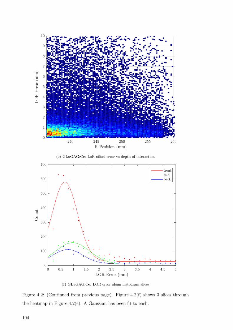
(e) GLuGAG:Ce: LoR offset error vs depth of interaction
(f) GLuGAG:Ce: LOR error along histogram slices
Figure 4.2: (Continued from previous page). Figure 4.2(f) shows 3 slices through
the heatmap in Figure 4.2(e). A Gaussian has been fit to each.
104

ErrorSource Centre Source 50% Inner Radius Source 75% Inner Radius
Q1 Median Q3 Q1 Median Q3 Q1 Median Q3
∆θ (Deg.) -0.26 -0.0019 0.25 -0.27 -0.0038 0.26 -0.28 -0.0029 0.27
∆r (mm) -3.07 0.33 1.22 -3.06 -0.33 1.21 -2.84 -0.31 1.11
∆z (mm) -0.92 -0.0050 0.93 -0.93 0.0038 0.99 -1.02 -0.0030 0.97
∆d (mm) 1.35 3.52 8.33 1.34 3.57 9.26 1.23 3.49 10.87
∆LoR (mm) 1.22 3.12 11.78 1.43 3.59 16.60 1.50 4.13 24.10
Table 4.4: LaF3:Ce-PS error statistics summary
4.3.2 LaF3:Ce-PS
Figure 4.3(a), 4.3(b) and 4.3(c) illustrate the error in radial, axial and rotational
dimensions for LaF3:Ce-PS. Overall error in endpoint location is shown in Figure
4.3(d), while Figure 4.3(e) shows the minimum distance from the estimated LOR
to the nominal centre of the radioactive source. Figure 4.3(f) shows three slices
through the LOR error heat-map (Figure 4.3(e)); the first at 10% of the scintillator
thickness (measured from the inner detector surface, R ≈ 239.4 mm), the second
at 50% of the scintillator thickness (R ≈ 256.7 mm) and the third at 90% of the
scintillator thickness (R ≈ 274.5 mm). A Gaussian function has been fitted to each
slice to indicate the accuracy of the LOR at these positions. The Gaussians have
been offset in Y to account for baseline noise. The R position on the horizontal
axis of each figure is the absolute radial distance from the centre of the scanner; the
range shown in the plots begins at the inner detector surface and ends at the outer
detector surface. Again, results for the offset source location are very similar.
A summary of the statistical range of the errors (first quartile, median and third
quartile) for LaF3:Ce-PS with the source in the same three positions (centre and
offset at 50% and 75% of inner shell diameter) is presented in Table 4.4. Statistics
for the total spatial error (∆d) have also been included.
4.3.3 Detector Sensitivity and Detection Accuracy
Table 4.5 presents a summary of the overall sensitivity of the two designs for each
source position, expressed as a fraction of positron annihilations which result in
detection of both endpoints, and the fraction of estimated endpoint locations which
105

(a) LaF3:Ce-PS: radial endpoint error vs depth of interaction
(b) LaF3:Ce-PS: axial endpoint error vs depth of interaction
Figure 4.3: LaF3:Ce-PS: endpoint errors in each dimension and overall vs. depth of
penetration.
106

(c) LaF3:Ce-PS: rotational endpoint error vs depth of interaction
(d) LaF3:Ce-PS: Total endpoint error vs depth of interaction
Figure 4.3: (Continued from previous page).
107

(e) LaF3:Ce-PS: LOR offset error vs depth of penetration
(f) LaF3:Ce-PS: LOR error along histogram slices
Figure 4.3: (Continued from previous page). Figure 4.3(f) shows 3 slices through
the heatmap in Figure 4.3(e). A Gaussian has been fit to each.
108
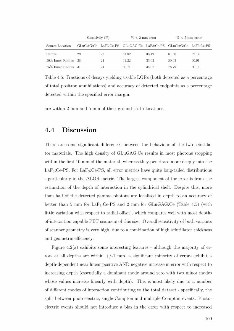
Sensitivity (%) % < 2 mm error % < 5 mm error
Source Location GLuGAG:Ce LaF3:Ce-PS GLuGAG:Ce LaF3:Ce-PS GLuGAG:Ce LaF3:Ce-PS
Centre 29 22 61.82 33.49 81.60 62.14
50% Inner Radius 28 21 61.22 33.62 80.43 60.91
75% Inner Radius 31 24 60.71 35.07 78.79 60.14
Table 4.5: Fractions of decays yielding usable LORs (both detected as a percentage
of total positron annihilations) and accuracy of detected endpoints as a percentage
detected within the specified error margin.
are within 2 mm and 5 mm of their ground-truth locations.
4.4 Discussion
There are some significant differences between the behaviour of the two scintilla-
tor materials. The high density of GLuGAG:Ce results in most photons stopping
within the first 10 mm of the material, whereas they penetrate more deeply into the
LaF3:Ce-PS. For LaF3:Ce-PS, all error metrics have quite long-tailed distributions
- particularly in the ∆LOR metric. The largest component of the error is from the
estimation of the depth of interaction in the cylindrical shell. Despite this, more
than half of the detected gamma photons are localised in depth to an accuracy of
better than 5 mm for LaF3:Ce-PS and 2 mm for GLuGAG:Ce (Table 4.5) (with
little variation with respect to radial offset), which compares well with most depth-
of-interaction capable PET scanners of this size. Overall sensitivity of both variants
of scanner geometry is very high, due to a combination of high scintillator thickness
and geometric efficiency.
Figure 4.2(a) exhibits some interesting features - although the majority of er-
rors at all depths are within +/-1 mm, a significant minority of errors exhibit a
depth-dependent near linear positive AND negative increase in error with respect to
increasing depth (essentially a dominant mode around zero with two minor modes
whose values increase linearly with depth). This is most likely due to a number
of different modes of interaction contributing to the total dataset - specifically, the
split between photoelectric, single-Compton and multiple-Compton events. Photo-
electric events should not introduce a bias in the error with respect to increased
109

depth, however, Compton-scattered events arriving at an oblique angle will tend
to scatter in approximately the angle of incidence. Therefore, if multiple energy
depositions occur they will tend to skew the estimated location, either positively or
negatively, depending on the precise nature of the scatter event.
A large part of the error is due to the implicit assumption that all detected
events are purely photoelectric, which is not true in practice. For both materials,
our simulations show that more than three quarters of all interactions between in-
cident gamma photons and the scintillator will be Compton-scattered, some more
than once (see Table 4.2). However, some of the scattered photons go on to entirely
escape the scintillator, while the subsequent interactions of many others often occur
close to the initial interaction. In these cases, if a non-trivial amount of energy is de-
posited, the fitting process will still work very well, since the total energy deposition
is one of the degrees of freedom of the optimiser. For multi-Compton interactions,
since scattering is biased towards the forward direction, it is more probable than
not that further interactions with the scintillator occur more deeply in the scintil-
lator shell, leading to more optical attenuation of the resulting scintillation photons
than for those produced during the initial interaction. This results in the observed
optical photon pattern being typically dominated by the first and shallowest inter-
action. The parametric fit to the analytic model is therefore quite similar to the
pure photoelectric case in many instances.
As expected for a PET system with high resolution DOI estimation capabilities,
degradation in localisation performance with increased radial displacement is quite
moderate, with the median error in LOR placement increasing from 1.27 mm to
1.62 mm between the centre and 75% of the inner radius of the cylindrical shell for
GLuGAG:Ce, and 3.12 mm to 4.13 mm in the case of LaF3:Ce-PS.
A direct comparison of the two materials suggests that GLuGAG:Ce is the su-
perior material. However, this does not account for economic factors which also
influence scanner design. The nanocomposite material has many desirable physical
and mechanical properties. If the performance is adequate for the targeted applica-
tion, it may very well be the more attractive material.
110

4.5 Conclusions and future work
This work established the feasibility of a continuous cylindrical shell PET scanner
based on either optically transparent ceramic garnet or inorganic scintillator/poly-
mer nanocomposite materials. Initial simulations for a point source located at three
positions within the scanner’s field of view are presented, yielding promising results
for the accuracy of detection of the endpoints of the line of response.
In the following chapters, we will develop a coincidence detection algorithm for
the proposed monolithic cylindrical shell scanner, and build a complete simulation
and STIR-based image reconstruction pipeline. We will evaluate the coincidence
detection sensitivity of the system and perform image reconstructions with point
sources at several different locations within the scanner’s field of view. The median
LOR displacement errors of 1.27-1.62 mm for GLuGAG:Ce and 3.12-4.13 mm for
LaF3:Ce-PS obtained in this study are suggestive of good performance in the next
phase of the project.
111

Chapter 5
Efficient spatio-temporal
deconvolution-based pulse pile-up
correction for coincidence
detection in monolithic-scintillator
PET systems
5.1 Introduction
In PET scanners utilising a continuous cylindrical shell of scintillator material, the
task of coincidence detection is necessarily very different to that in classical PET.
Rather than a situation in which most or all optical photons resulting from gamma
photon energy deposition will be collected by a small subset of pixels in the photode-
tector array (depending on the optical coupling between scintillator and photode-
tectors), where a simple time-windowed binary AND-gate approach can be used for
coincidence detection, coincidences in a continuous cylindrical shell scanner manifest
as near-simultaneous bursts of optical photons which are detected on the inner and
outer surface of the scintillator shell across a variable number of pixels. The produc-
tion of these photons is not instantaneous; rather, following the interaction, they are
progressively emitted with an emission intensity that rapidly rises and slowly decays
according to a a multi-exponential function of time. The onset of these photon bursts
112
is determined by the time of flight of each half of the coincidence; depending on the
activity in the object being imaged and the decay time of the scintillator, unrelated
individual optical photon showers have a certain probability of overlapping, both
in space and time. If it is possible to isolate and cluster individual photon showers
as belonging to a single annihilation based on the spatio-temporal relation of the
arriving optical photons, then it should be possible to utilise the methods presented
in Chapter 4 to localise the endpoints of the line of response and incorporate it into
the projection sinogram [171].
The problem of resolving individual photon showers in monolithic PET systems
is analogous to the one-dimensional problem of pulse pile-up in classical nuclear
spectroscopy, which has previously been addressed via temporal deconvolution of
the composite signal by the impulse response of the scintillator to resolve the piled-
up pulses as a string of quasi-instantaneous impulses (Dirac delta functions) [172].
In fact, if the signals from multiple individual photodetectors are added together, the
ensemble can be thought of as a large single-channel detector. Due to the limited
scintillator thickness (typically less than 30 mm), the specific depth of the point
of interaction within the slab has a minimal impact on the pulse shape (since the
maximum realistic optical photon path in the scintillator will be traversed in about
100-200 ps, compared to a minimum decay time in LSO of 20-50 ns [173, 174]).
The pulse amplitude depends on the amount of energy deposited by the interaction,
but the shape is always essentially the same. Therefore, it should be possible to
successfully deconvolve the summation signal by a representative temporal impulse
response to achieve good temporal pulse resolution.
This Chapter introduces a deconvolution-based method for identifying coinci-
dences in continuous-shell cylindrical PET scanners. Statistical results from the
application of this method to a Monte Carlo simulation are calculated and com-
pared to the ground truth coincidence data obtained directly from the simulation.
By implementing this method for coincidence detection in combination with the line-
of-response endpoint localisation algorithm described in the previous Chapter, all
of the essential infrastructure required for constructing PET lines of response and
hence generating data for image reconstruction is available for a continuous-shell
cylindrical PET system.
113

5.2 Materials and Methods
The methods described in this Section can be applied to any scanner with a con-
tinuous cylindrical shell and two-sided (inner and outer surface) optical detection.
The specific geometry used for the Monte Carlo simulation evaluation of the pro-
posed technique, and the simulation parameters themselves, are described in detail
in Section 5.2.5 and 5.2.6, respectively. It is assumed that the optical photon counts
in each pixel (both on the inside and outside of the shell) are periodically read out
digitally, logged and reset via a synchronous clock signal which is simultaneously
distributed to all detector modules via equal-length transmission paths.
5.2.1 Coincidence Detection Technique
The inner and outer detector surfaces are each divided into an integral number of
sectors, with equal angular coverage in each sector (see Figure 5.2). The identity of
any photodetector pixel in which a non-zero number of optical photons is detected
in each clock cycle is converted into a cylindrical coordinate system and assigned to
one of these sectors; in the specific geometry evaluated in this work, 16 sectors, each
of 22.5°, were used. To capture interactions which may fall along the edges of the
angular sections, the same data was also assigned to a second set of “offset sectors”,
which are the same size but offset by half of the sector width. Photon showers which
lie on a sector boundary in one sector set will therefore be in the centre of a sector
in the alternate set.
5.2.2 Impulse Response Generation
A centrally located periodic 10 MBq 18F-like pseudo-source was simulated, and a
sample of 1000 decays was generated. Photoelectric interactions were then identified
via the amount of energy deposited by primary gamma photons, and the optical
scintillation photons resulting from these primaries were grouped together as they
arrived at the photodetectors, summed and logged at each time sample, resulting in
a single time-domain waveform for each. The depth of interaction was also recorded
for each photoelectric interaction; the radial dimension of the ring in this case was
quantised into five 5 bins, with the minimum and maximum allowable positions
114
being the apothem of the inner and the radius of the outer polygon surfaces. The
resulting time-domain waveforms were separately averaged for each of the five depth
ranges, resulting in a representative mean impulse response at each depth (see Figure
5.1). The impulse responses were also amplitude-normalised (since interactions in
the middle of the cylindrical shell will tend to result in smaller-amplitude optical
pulses compared to those interacting near the inner or outer surface of the shell).
As expected, due to the relatively short photon propagation time relative to
the scintillator decay constants, little variation is observed between photoelectric
impulse responses at different depths (Compton events where some part of the initial
photon energy escapes will also have a similar shape, but lower amplitude). This
impulse response is used as the deconvolution kernel for the coincidence detection
algorithm.
5.2.3 Single, 2-Coincidence and Multiple-Coincidence De-
tection
Synchronous readout from any pixels registering hits is performed at 10 ns intervals
(comparable to the typical timing window of 6-12 ns in conventional PET systems
[10, 175, 176]) and summed in each sector and offset sector to yield a set of time-
domain signals (32 signals for this specific geometry). Each signal is deconvolved
with the mean scintillator impulse response (see Figure 5.3), greatly reducing the
pulse pile-up and cleanly separating most of the impulses.
In each time slice, a threshold of 5% of the maximum amplitude of a single
photoelectric impulse is applied to each of the deconvolved waveforms. The type of
event may then be distinguished by the number of channels where the amplitude
exceeds the threshold. If only a single channel exceeds the threshold, the event
is logged for potential use in the randoms correction procedure. If exactly two
channels register, then the event is considered a potential coincidence and logged
for further analysis. If more than two channels exceed the threshold, the event is
recorded as a ‘multiple-interaction event’ but not used for image reconstruction as
it is not possible to determine which two events should be used as the endpoints of
the line of response. The choice of 5% for the threshold is largely arbitrary, and the
method still works over a wide range of threshold values; however, this is a tunable
115

(a) Impulse response generation: raw intensity
(b) Impulse response generation: normalised intensity
Figure 5.1: The generated impulse responses for five discrete radial bins. The bins
are numbered 1 (closest to inner detector surface) to 5 (closest to outer detector
surface).
116

parameter which may be adjusted if desired (a higher threshold will result in a lower
rate of false positives, but lower overall sensitivity). Importantly, if one particular
channel registers an event, and either (or both) of its immediate half-sector-offset
neighbours also registers an event, the smaller event/events is/are ignored as it/they
are assumed to be due to the same event (since the imaging object cannot fill the
entire field of view, and it would need to almost touch the ring if it were to register
a true coincidence in adjacent half-sectors).
The time samples in which a potential coincidence event has been identified
signify the onset of the event, since the deconvolution process fully equalises the
impulse response of the scintillation process - ideally, concentrating the energy of
the event into a single instant (the time of arrival of the original gamma photon).
The next step is temporal segmentation of the original optical photon arrival signals
to the interval surrounding each event, and spatial segmentation to identify the
location of the point of interaction.
Following identification of the onset of an event in the deconvolved waveforms at
time tc, the original (i.e. not deconvolved) signals from each detector are extracted
between tc ≤ t ≤ tc + τ , where τ is the duration of the impulse response (time to
fall to 5% of the maximum value; approximately 3 time constants) and summed in
the time dimension, resulting in a two-layered cylindrical image of all photons cap-
tured within the emission timing window. The global maximum is located, and the
circular (or part-circular, for maxima near the axial extrema of the image) region
surrounding this maximum with a radius determined by (4.3) and (4.4) is copied
and then masked out (zeroed) on both layers. This process is then repeated (post-
masking) as required, depending on the number of simultaneous events which have
been identified as occurring within this sample period (i.e. based on the number of
deconvolved signal channels exceeding the threshold), since the only remaining max-
imum should correspond to the other end of the line of response. The mask is also
applied to the complete dataset, preventing the decaying pulses which commenced
in the current sample from registering again in the samples immediately following,
since the decaying pulse may still exceed the amplitude of these subsequent pulses.
Depending on the number of photon clusters thus identified, the image subsets are
copied into one of the time-ordered vectors of either single, coincidence and multiple
117
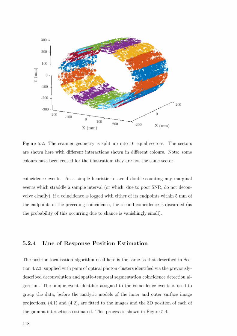
Figure 5.2: The scanner geometry is split up into 16 equal sectors. The sectors
are shown here with different interactions shown in different colours. Note: some
colours have been reused for the illustration; they are not the same sector.
coincidence events. As a simple heuristic to avoid double-counting any marginal
events which straddle a sample interval (or which, due to poor SNR, do not decon-
volve cleanly), if a coincidence is logged with either of its endpoints within 5 mm of
the endpoints of the preceding coincidence, the second coincidence is discarded (as
the probability of this occurring due to chance is vanishingly small).
5.2.4 Line of Response Position Estimation
The position localisation algorithm used here is the same as that described in Sec-
tion 4.2.3, supplied with pairs of optical photon clusters identified via the previously-
described deconvolution and spatio-temporal segmentation coincidence detection al-
gorithm. The unique event identifier assigned to the coincidence events is used to
group the data, before the analytic models of the inner and outer surface image
projections, (4.1) and (4.2), are fitted to the images and the 3D position of each of
the gamma interactions estimated. This process is shown in Figure 5.4.
118

(a) Coincidence detection: unprocessed signal
Coincidence
Coincidences
Single
Singles SingleSingle
(b) Coincidence detection: deconvolved signal
Figure 5.3: Deconvolution is used to reduce pulse pile-up between events and prop-
erly resolve coincidence pairs. A coincidence pair is recorded if two peaks are within
the same 10 ns sample interval and intensity is above 5%-of-maximum threshold
(dashed line). The different colours correspond to different sections of the cylinder.
119

Figure 5.4: Line of response generated from a single coincidence detection, using
optical photon distributions captured on the inner and outer detector surfaces. Each
face of the inner and outer surfaces of these pseudo-cylindrical polyhedral shells
represents a row of 21 SiPM detectors, with scintillator material sandwiched between
the inner and outer detectors. The dark blue and orange points correspond to the
annihilation photons detected on the inner surface and outer surfaces, respectively.
The three small black cylinders inside the ring represent 18F sources and water
phantoms. The source generating the LOR is positioned at the centre of the field of
view, while the other two are offset in the radial dimension by 50% and 75% of the
inner surface radius.
120
5.2.5 Geometry
The geometry of the scanner is the same as that which is described in Section 4.2.2.
Only the GLuGAG:Ce ceramic scintillator is used in these simulations, since this
material was previously shown to offer the best performance amongst the evalu-
ated scintillators - however, a scanner can be designed with an optimal scintillator
thickness using any of the ceramic or nanocomposite materials. In summary, the
scintillator is a polygonal (pseudo-cylindrical) shell, where the inner polygon has 104
14.442 mm faces and the outer polygon has 110 14.2 mm faces. Each of the polygon
faces is optically coupled to a row of 21 12×12 pixel SiPM arrays (the geometry is
shown in Figure 4.1). The pixel pitch of the SiPM arrays is 1 mm in both dimen-
sion (with an assumed 100% fill factor in the array), while a 1 mm insensitive area
surrounds the array, with an additional axial separation between SiPMs of 0.1 mm,
resulting in a total axial length of 296 mm.
3 MBq 18F sources were placed at three positions inside the scanner: one in the
centre of the field of view, and two more offset in the radial dimension by 50% and
75% of the inner surface radius. The axial position in each case was at the centre
of the scanner. The sources were each cylindrical with a radius of 1 mm and height
of 2 mm, and were each placed within a cylindrical water phantom of radius 5 mm,
height 10 mm.
Separate simulations were performed for scanner normalisation; these are de-
scribed in Chapter 6.
5.2.6 GATE Simulation Parameters
GATE version 8.1 [160, 161] and Geant4 version 10.4p02 [162] are used for all sim-
ulations. Full optical photon tracking was enabled on all simulations.
The polyhedral prismatic scintillator shell was designed in OpenSCAD and ex-
ported as a stereolithography (STL) file. It was then included in the GATE sim-
ulation using the “tessellated” volume option, which allows an STL file to be used
as a geometric object. Optical properties for GLuGAG:Ce and meltmount optical
coupling epoxy were taken from the literature [118, 167, 164]. Other physical compo-
nents in the simulation employed standard GATE materials and surface properties.
The simulation was performed with the scintillator as a ‘sensitive volume’, so that
121

True Detections (%) 17.42 ± 0.13
Random Detections (%) 2.08 ± 0.07
Missed Detections (%) 15.37 ± 0.30
Total Interactions (%) 32.79 ± 0.21
Table 5.1: The proportion of true (true positive), random (false positive) and missed
(false negative) detections as a percentage of the total number of decays. Results
are expressed as the mean and standard error of the mean, after five repeats of the
simulation.
the exact location and type of each interaction between the gamma photons and the
scintillator could be absolutely determined. This allows the number of apparent
coincidences (as detected by the coincidence detection algorithm) to be compared
against the ground truth (cases where both photons interacted with the scintillator
volume) such that false positives (randoms) and false negatives (missed true coin-
cidences) can be quantified. An event (identified by a unique event ID) is classified
as a true coincidence if two primaries are produced with different “track IDs” but
with a “parent ID” equal to 1 (the ID of the original positron particle). Coinci-
dences may also be classified as photoelectric-photoelectric (PE-PE), photoelectric-
Compton scattered (PE-CS) or Compton scattered-Compton scattered (CS-CS) to
determine the impact of the interaction type on the accuracy of the classification
algorithm. Due to the resources involved in tracking optical photons in such a
large sensitive volume, the number of primary decays is limited to 9000, and the
simulation was repeated five times.
5.3 Results
5.3.1 Algorithm Detection Efficiency
Table 5.1 shows the proportion of true, random and missed coincidence detections
as a percentage of the total number of positron decays.
True coincidences detected are 53.13% of the total number of interactions which
actually occur. The random fraction is 0.1062.
122

PE-PE PE-CS CS-CS
Type of Interaction (%) 6.24 ± 0.22 37.71 ± 0.50 56.04 ± 0.36
Interactions Detected (%) 52.71 ± 1.38 53.27 ± 0.80 53.06 ± 0.57
Table 5.2: The proportion of each detection type as a percentage of the total number
of true detections and the detection percentage. Random events are not included.
5.3.2 Detection Efficiency by Interaction Type
Table 5.2 shows the proportion of coincidence detections which are photoelectric-
photoelectric (PE-PE), photoelectric-Compton scattered (PE-CS) and Compton
scattered-Compton scattered (CS-CS), by ground truth knowledge from GATE. The
detection rate of each type is also calculated. All three types of events are quite
similar (certainly within the error margin of each other), with PE-PE being the
lowest at 52.71% and PE-CS the highest at 53.27%.
5.4 Discussion
The shape of the scintillator impulse response is very consistent, regardless of the
depth of interaction within the crystal. However, the amplitude strongly depends on
the nature of the interaction (either deposition of all of the gamma photon energy
via photoelectric interactions, or partial energy deposition via Compton interactions)
and the depth at which the energy is deposited (due to scattering and attenuation
in the scintillator). The amplitude of the impulse response is a minimum for inter-
actions whose depth is half the thickness of the cylindrical shell. These observations
confirm the basic validity of the proposed approach.
The solid angle coverage of the simulated scanner geometry limits the proportion
of decays which can be detected as a true coincidence to ∼32%, which is in close
agreement with the results presented in table 4.5. Of this fraction of potentially
detectable coincidences (which could be improved with increased solid angular cov-
erage), including coincidences in which one or both interactions scatter following
Compton interactions in the scintillator and which only deposit a small fraction of
the incident photon’s energy there, a little over half are classified as coincidences
by the proposed algorithm, and hence will contribute to the sinogram, while the
123

others deposit too little energy in one or both halves of the coincidence to register.
In a comparable discrete-crystal PET system, most coincidences which fail to be
detected here would also be outside of the scanner’s energy window and therefore
not contribute to the sinogram.
In Chapter 3 the proportion of interactions which were photoelectric was ∼24%
for the GLuGAG:Ce ceramic scintillator, so figures quoted in the first row of table
5.2 are close to the expected values (PE-PE coincidences are expected to occur with
a probability of 0.24 × 0.24 or about 6%, PE-CS or CS-PE coincidences 0.24 ×
(1 − 0.24) × 2 or about 36% and CS-CS coincidences (1 − 0.24)2 or about 58%).
The probability of detecting a true coincidence is better than 50% for all types of
interaction. The failed detections usually correspond to cases in which either there
was a multiple interaction at one endpoint (and hence the event was discarded,
as would be the case in a classical pixellated-scintillator system), or one or both
interactions near one end of the cylindrical scintillator shell, in which case too many
photons may be lost for reliable classification.
5.5 Conclusion
This work introduced a spatio-temporal deconvolution and segmentation algorithm
for PET systems based on large monolithic scintillators. When applied to a novel
cylindrical-shell monolithic PET architecture, it was found that more than half
of the potentially detectable true coincidence events could be correctly identified
detected, with a random fraction of 10.62%. It was also found that both Compton-
photoelectric and Compton-Compton coincidence pairs could be detected with a
sensitivity approximately equivalent to that for photoelectric-photoelectric interac-
tions.
The proposed algorithm identifies a sufficient fraction of true LORs to enable
practical image reconstruction; the next Chapter will describes how these LORs
are used to reconstruct a 3D image using a range of analytic techniques and image
reconstruction algorithms.
124

Chapter 6
Design and Simulation of a Brain
PET Scanner with a Continuous
Cylindrical Shell Monolithic
Scintillator
6.1 Introduction
Clinical PET scanners currently in use tend towards a common design structure
- they use rectangular blocks of discrete scintillator crystal arrays, optically cou-
pled to either photomultiplier tubes or silicon photomultipliers (SiPMs), completely
surrounding the patient in a ring. This configuration has worked well for decades,
although a major limitation still exists: the spatial resolution of the system is fun-
damentally tied to the dimensions of the elements in the scintillation detector array.
A “hit” is recorded on a detector element if an interaction triggers a light yield
above a certain energy threshold, though there is no way to explicitly determine
exactly where the interaction occurred within the scintillator volume, only that it
did occur. If two detector elements are triggered at approximately the same time,
then a coincidence is said to occur and a line of response can be drawn between the
two elements. A typical system might contain scintillation crystals approximately
4 mm×4 mm×22 mm [2], hence most modern systems achieve a spatial resolution
somewhere in the vicinity of 3-5 mm for full body systems and 1-2 mm for small
125

animal systems [23].
A high spatial resolution is important in both diagnostic imaging and biologi-
cal research applications of PET, since more image detail in fine structures is re-
vealed, allowing for more conclusive diagnoses and stronger scientific conclusions to
be drawn from an image. A key hypothesis for the development of a fully mono-
lithic, cylindrical PET detector architecture, was that the design would allow for the
spatial resolution to be improved because it is no longer limited by the dimensions
of the scintillator crystal; rather it is based on the statistical methods which esti-
mate the position at which the emitted gamma photon interacts with the detector
(as described in Chapter 3.2). Each location is estimated by analysing an optical
photon map and fitting an analytic function to the data to find the most likely three
dimensional position for the location of the interaction. After exploring solutions to
coincidence detection and LOR determination for such a radical architecture in the
previous two Chapters, it is now possible to combine each of the proposed meth-
ods with several standard image reconstruction techniques to generate a complete
image, with all necessary corrections applied.
In this Chapter a full optical simulation of three 3 MBq 18F radioactive sources
is performed using the Geant4 Application for Tomographic Emission (GATE) [160,
161]. For the first time, image reconstruction is achieved using several image recon-
struction methods implemented in the well-known Software for Tomographic Image
Reconstruction (STIR) package [156]. A number of standard corrections were first
applied before the spatial resolution is estimated via measurement of the FWHM
for each source in each dimension. This work aims to provide a basic proof of con-
cept and validate the entire end-to-end signal processing pathway for the proposed
scanner design.
Section 6.2 describes the methodology used for image reconstruction and correc-
tion, as well as the specific parameters and algorithms used; the parameters used
in the optical simulation, which has generated the data for the reconstruction, are
also discussed. Section 6.3 presents the results of the image reconstructions, with
important observations discussed in Section 6.4. Finally, Section 6.5 concludes the
chapter by summarising the key findings and outlining possible next steps for the
continuation of the study.
126

6.2 Materials and Methods
6.2.1 Simulation Parameters
The fully monolithic continuous cylindrical shell scanner geometry is exactly the
same as previously described in Section 4.2.2 and Section 5.2.5. GLuGAG:Ce ce-
ramic garnet is again used as the scintillation material and meltmount has been
modelled as the material used for optical coupling to the silicon photomultiplier ar-
rays. Physical properties of the scintillator and other optical components have been
obtained from the literature [118, 167, 164].
The simulation has again been performed in GATE version 8.1 [160, 161] with
Geant4 version 10.4p02 [162]. Full optical tracking was enabled for all simulations,
with the exception of the simulation used to generate normalisation data. In the
main simulation, three 3 MBq 18F sources were used, each modelled as a short cylin-
drical source with a diameter of 2 mm and height of 2 mm, positioned at the centre
of the scanner FOV and offset in the radial dimension by 50% and 75% of the inner
surface radius. Each of these sources were contained in a cylindrical water phantom
with a radius of 5 mm and a height of 10 mm, to ensure all emitted positrons would
annihilate but without inducing significant amounts of scattering. List-mode data
was acquired with these sources over a period of 3 seconds of simulation time, giving
a total of approximately 27 million decays.
For normalisation, a phantom of radius 233.315 mm and height 296 mm filled
with a solution of 18F in water is situated in the centre of the FOV of the scanner.
Five billion events were simulated as primaries only (data collection and storage for
an optical system is much too great for such a large number of events). The reasons
for this approach will be discussed in detail in subsequent sections.
6.2.2 Image Reconstruction
STIR version 3.0 [156] was used for all image reconstructions. Since the geometry
of the scanner is quite different to that normally used with STIR, some additional
preprocessing steps are needed to convert the listmode data into a format which
can be read by STIR and properly processed. The first tool [177] generates a pixel-
lated cylindrical map of virtual detector locations within the scanner, based upon
127

input geometrical specifications, using a similar approach to that of Li et al., and
Scheins et al. [52, 178]. The map is essentially a zero-thickness virtual cylinder;
the two intersection points of each LOR are calculated, quantised and then mapped
to the pixels of each virtual detector surface. This approach enables the continu-
ous depth of interaction (DOI) estimate produced by the LOR endpoint estimator
to be mapped to a single layer for image reconstruction, speeding up image recon-
struction and greatly reducing memory consumption compared to a multi-layer DOI
quantisation approach. The pixel dimensions in the virtual cylinder are arbitrarily
chosen according to the desired trade-off between spatial resolution and signal to
noise ratio (and image reconstruction time - a higher resolution virtual cylinder will
greatly extend the time and memory required for image reconstruction, particularly
for iterative algorithms).
In this work, the size of the virtual ring is equal to the length of the scanner
(296 mm), with radius equal to the inner face of the detector ring (apothem of the
inner polygon = 233.31 mm). There were 77 virtual rings along the axial length of
the scanner, each containing 384 detector elements around the circumference. The
number of voxels used in image space was 245×245×153 (in x, y, and z dimensions,
respectively). The dimensions of each voxel are 1.922 mm×1.922 mm×1.922 mm.
Once mapped, the data is converted from ASCII text into SAFIR listmode
format- a custom binary format which has been integrated into the STIR library for
conversion into Interfile sinogram format [179, 180]. Re-sampling the LOR data in
this manner requires an input sinogram header, which specifies the scanner param-
eters. The parameters used for this scanner geometry are listed in Table 6.1, and
have been generated via STIR’s inbuilt create projdata template function. Once the
sinogram was produced, both analytic and iterative reconstruction algorithms were
applied; specifically 2-D Filtered Back Projection (with single-slice rebinning), 3-D
Filtered Backprojection with Reprojection and the Ordered Subsets Maximum A
Posteriori - One Step Late (OSMAPOSL) algorithm, configured as simple OSEM
(i.e. there was no a priori image and instead a flat image of zeros was used). OSEM
was configured to operate with 8 subsets and 30 sub-iterations. The ramp filter used
in FBP2D had an alpha parameter of 1 and cut-off frequency of 0.5. The Colsher
filter used in FBP3DRP similarly used an alpha value of 1 and cut-off frequency of
128

0.5 in both the axial and planar dimensions.
All images presented in this Chapter have been produced using AMIDE to display
image-domain Interfile data. AMIDE was also used to produce line profiles and
measure the full width at half maximum (FWHM) from the point source images.
The FWHM is measured for all sources in three dimensions, using zero as a reference
point for the measurement (the analytic reconstructions produced small negative
values in some instances).
6.2.3 Image Correction
Various corrections have been applied to the reconstructed images. Most of these
operations are performed in the projection (sinogram) space, then the selected re-
construction algorithm is applied to the corrected sinogram afterwards. Equation
(6.1) details the process by which the raw sinogram is generated and which should
be corrected to restore the forward-projected emission sinogram as accurately as
possible (and hence enable proper image reconstruction in the spatial domain):
sinogram (uncorrected) =fwd(emission) + (norm× ACF × (random+ scatter))
norm× ACF(6.1)
where fwd(emission) is the exact forward projection of the emission image,
norm is the attenuation-corrected sinogram acquired from a uniformly-filled phan-
tom (or equivalently, generated using a component-based normalisation scheme),
ACF is the attenuation correction factor sinogram, and random and scatter are
the uncorrected sinograms resulting from random coincidences and scatter events,
respectively.
To recover an accurate estimate of the forward-projected emission sinogram, the
uncorrected sinogram is first multiplied element-by-element by a smoothed normal-
isation sinogram which encompasses the entire FOV of the scanner, and the ACF
sinogram (which, in practice, is computed by converting the Hounsfeld units of
a CT image into an estimated attenuation coefficient at 511 keV). The additive
contributions from random and scattered events are then corrected by subtracting
their normalised and attenuation-corrected sinograms; random correction is nor-
mally performed using a delayed coincidence channel (which can completely exclude
129

Material GLuGAG:Ce
Number of detectors per ring 384
Number of rings 77
Default tangential Positions 245
Inner ring radius (mm) 234.97
Average DOI (mm) 0.01
Ring spacing (mm) 3.84
Tangential bin size (mm) 1.92
Intrinsic tilt (degrees) 0
Transaxial blocks per bucket 1
Axial blocks per bucket 1
Axial crystals per block 1
Transaxial crystals per block 1
Axial crystals per singles unit 1
Transaxial crystals per singles unit 1
Detector layers per block 1
Mash factor 1
Arc corrected No∗
Tangential positions 245
Span value 1
Max. ring difference 76
Table 6.1: Parameters used in STIR’s create projdata template. ∗ indicates that arc
correction will be done later as part of the FBP2D or FBP3DRP algorithms. The
Interfile code used for this particular scanner is included in Appendix A.2.
130

the possibility of any true coincidences being present) while scatter correction can be
performed by performing a tail-fitting procedure on the image or by energy window-
ing to restrict the photons used in image reconstruction to non-scattered photons).
The sinograms used for normalisation, attenuation and randoms correction and
their reconstructed images are shown in Figure 6.1. Each have been reconstructed
using FBP3DRP. For the specific point-source simulations performed in this work,
only a very small volume of water surrounds each point source (to ensure that
the positrons annihilate); therefore, scattering is negligible and not included here
(although the standard methods for scatter correction are applicable).
Each of the correction terms is discussed in more detail in the following sections,
with the exception of scatter correction, which is not performed.
Random Correction
Random correction is performed on the data using a variation of the well-known de-
layed window technique [181]. Once single events, coincidence events and multiple
events have been identified and classified into their own respective datasets using the
coincidence identification technique discussed in the previous Chapter, the singles
dataset is used to generate random coincidence data, using a variation of the coin-
cidence detection method described previously in Section 5.2.1. To implement the
delayed-coincidence method, we consider ‘random’ coincidences to be those where
detected singles are separated by a number of timing bins equal to a time greater
than the decay time of the scintillator. Specifically, the fixed separation time be-
tween pulses is equal to the time taken for the photoelectric impulse response to
decay to less than 5% of its maximum energy; for GLuGAG:Ce this is 300 ns or 30
10 ns bins (rounded up to the nearest bin).
A logical array (with axes of sector number and timing bin) is once again used
to identify coincidences. In the ‘true’ coincidence detection method, a coincidence
was identified when two sections flagged an event in the same timing bin. Using a
delayed window means that a single event in one timing bin must be paired with
another which is both in a different sector and exactly delayed by a fixed interval
of 300 ns. The method used was to duplicate the array, offset it by the decay time
and then add the two arrays together, again looking for coincidences which were in
131

(a) Projection space: randoms correction. (b) Image space: randoms correction.
(c) Projection space: normalization correc-
tion.
(d) Image space: normalization correc-
tion.
(e) Projection space: attenuation correction. (f) Image space: attenuation correction.
Figure 6.1: Sinograms (a), (c), (e) and Transaxial image slices (b), (d), (f) of the
correction factors. Images reconstructed using the FBP3DRP analytic algorithm.
132

different sectors. These may then be processed as normal with the LOR position
estimation algorithm. The resulting LORs are then processed in the same manner
as outlined in Section 6.2.2, to produce the required sinogram.
Attenuation Correction
An attenuation map (or mu-map) must be generated based on the structure and
composition of the imaging object. This can be done entirely within the STIR en-
vironment by using the generate image function. Each of the three 18F sources
is completely contained within a compact cylindrical water phantom; the atten-
uation map equals 0.096 cm−1 within the water volume and 0 cm−1 everywhere
else (for the air inside the FOV). The output image file contains voxels of size
245×245×153 (in x, y and z dimensions, respectively), which are each approximately
1.922 mm×1.922 mm×1.922 mm in size. Once the attenuation map is constructed,
it is used as an argument in STIR’s calculate attenuation coefficients function with
the –ACF option flagged, to calculate the attenuation correction factor for each of
the voxels on the attenuation map. This last step outputs a sinogram, in Interfile
format, which is then used to perform attenuation correction on the image in the
projection (sinogram) domain.
Normalisation
Due to the computational workload of conducting a simulation of sufficient fidelity of
a flood-filled source with full optical photon tracking is not feasible. This would not
be an issue for a physical scanner (where a normalisation scan must be performed
periodically as a routine part of scanner maintenance); however, for this work, it is
necessary to obtain the normalisation sinogram via an expedited simulation. There-
fore, a cylindrical phantom, filled with an 18F solution and encompassing almost
the entire FOV of the scanner, is simulated in GATE with optical photon tracking
disabled.
The exact locations of the first points of interaction between all 511 keV photons
and the scintillator volume are recorded. Coincidences were identified by examining
the “Event ID” number of these photons to identify pairs of annihilation photons
originating from the same annihilation event. The two lowest “Track IDs” were used
133

to find the locations and times corresponding to the the first points of interaction
(disqualifying cases where Track ID equalled the Parent ID of another interaction
of the same event ID - these are subsequent interactions of the same photon). After
the two endpoints of the LOR are found, they are recorded in a format which
may be processed using the image reconstruction procedure outlined in Section
6.2.2. Following reconstruction, the normalisation sinogram essentially resembles
that which would be obtained if a full optical simulation were performed, with the
chief difference being that due to the exactness with which the points of interaction
are known, the signal to noise ratio (SNR) of the resulting sinogram will be higher
for the number of simulated decays. Since a normalisation sinogram should have as
high an SNR as possible, this is beneficial to the image reconstruction process.
6.3 Results
6.3.1 Image Reconstruction
Figures 6.2, 6.3 and 6.4 are the reconstructed images of the three 18F sources, using
2D-FBP, 3D-FBPRP and OSEM algorithms respectively. In each figure, subfigures
(a), (c) and (e) are the raw (uncorrected) reconstructions in the transverse (x −
y), coronal (x − z) and sagittal (y − z) planes, while subfigures (b), (d) and (f)
are the corresponding images following normalisation and random and attenuation
corrections.
6.3.2 Spatial Resolution Measurements
Figures 6.5 and 6.6 are line profiles taken from Figure 6.2. Figure 6.5 depicts an
intensity profile of the line of voxels running horizontally through the centre of the
transverse plane (x dimension), while the subfigures in Figure 6.6 correspond to
pixels running through the centre of each source, vertically through the transverse
plane (y dimension) and vertically through the coronal plane (z dimension). Simi-
larly, Figures 6.7 and 6.8 are line profiles taken from Figure 6.3, and Figures 6.9 and
6.10 are line profiles taken from Figure 6.4. Profiles of both the raw (uncorrected)
images as well as the corrected data sets (normalised, and corrected for randoms and
134

(a) Uncorrected transverse plane (b) Corrected transverse plane
(c) Uncorrected coronal plane (d) Corrected coronal plane
(e) Uncorrected sagittal plane (f) Corrected sagittal plane
Figure 6.2: 2D analytic image reconstruction of three 3 MBq 18F sources encapsu-
lated in cylindrical water phantoms, using STIR’s FBP2D algorithm.
135
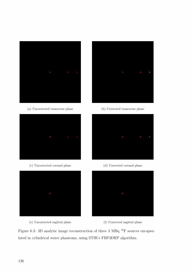
(a) Uncorrected transverse plane (b) Corrected transverse plane
(c) Uncorrected coronal plane (d) Corrected coronal plane
(e) Uncorrected sagittal plane (f) Corrected sagittal plane
Figure 6.3: 3D analytic image reconstruction of three 3 MBq 18F sources encapsu-
lated in cylindrical water phantoms, using STIR’s FBP3DRP algorithm.
136

(a) Uncorrected transverse plane (b) Corrected transverse plane
(c) Uncorrected coronal plane (d) Corrected coronal plane
(e) Uncorrected sagittal plane (f) Corrected sagittal plane
Figure 6.4: 3D iterative image reconstruction of three 3 MBq 18F sources encapsu-
lated in cylindrical water phantoms, using STIR’s OSMAPOSL algorithm.
137

Figure 6.5: Intensity profile of the FBP2D-reconstructed image. The slice is taken
along the x axis in the transverse plane of the scanner.
attenuation) have been overlaid for comparison. Tables 6.2, 6.3 and 6.4 summarise
the FWHMs of each of the source intensities in x, y, and z dimensions, respectively.
Each table compares all image reconstruction algorithms and the effect of image
corrections on the results.
Recon.Algorithm
FWHM - Centre (mm) FWHM - 50% Rad. (mm) FWHM - 75% Rad. (mm)
Uncorr. Corr. Uncorr. Corr. Uncorr. Corr.
2D-FBP 3.50 ± 0.52 3.71 ± 0.33 3.85 ± 0.81 3.88 ± 0.33 3.50 ± 0.99 3.10 ± 0.38
3D-FBP 3.29 ± 0.71 3.27 ± 0.50 4.09 ± 1.43 4.03 ± 0.76 3.69 ± 1.62 3.48 ± 0.61
OSEM 3.38 ± 0.32 3.36 ± 0.23 3.95 ± 0.59 3.95 ± 0.35 3.94 ± 0.75 3.84 ± 0.30
Table 6.2: Full width at half maximum (FWHM) of the intensity profiles at zero
degrees in the transverse plane (x-axis of the system).
138

(a) Centre source (y-axis) (b) Centre source (z-axis)
(c) 50% rad. source (y-axis) (d) 50% rad. source (z-axis)
(e) 75% rad. source (y-axis) (f) 75% rad. source (z-axis)
Figure 6.6: Intensity profile of the FBP2D-reconstructed image. The slices are taken
along the y and z axes, vertically, in the transverse and coronal planes of the scanner,
respectively.
139
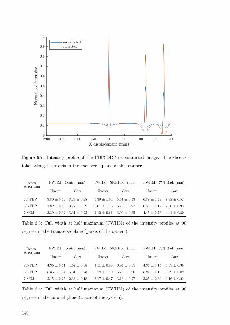
Figure 6.7: Intensity profile of the FBP3DRP-reconstructed image. The slice is
taken along the x axis in the transverse plane of the scanner.
Recon.Algorithm
FWHM - Centre (mm) FWHM - 50% Rad. (mm) FWHM - 75% Rad. (mm)
Uncorr. Corr. Uncorr. Corr. Uncorr. Corr.
2D-FBP 3.80 ± 0.52 3.23 ± 0.28 5.39 ± 1.04 5.51 ± 0.43 6.88 ± 1.43 8.32 ± 0.52
3D-FBP 3.82 ± 0.85 3.77 ± 0.59 5.61 ± 1.76 5.76 ± 0.97 6.35 ± 2.19 7.30 ± 0.93
OSEM 3.39 ± 0.32 3.31 ± 0.22 4.10 ± 0.61 3.99 ± 0.35 4.45 ± 0.76 4.41 ± 0.30
Table 6.3: Full width at half maximum (FWHM) of the intensity profiles at 90
degrees in the transverse plane (y-axis of the system).
Recon.Algorithm
FWHM - Centre (mm) FWHM - 50% Rad. (mm) FWHM - 75% Rad. (mm)
Uncorr. Corr. Uncorr. Corr. Uncorr. Corr.
2D-FBP 4.35 ± 0.61 4.52 ± 0.38 4.11 ± 0.88 3.94 ± 0.35 4.36 ± 1.15 4.39 ± 0.39
3D-FBP 5.35 ± 1.04 5.31 ± 0.73 5.78 ± 1.79 5.75 ± 0.96 5.94 ± 2.19 5.89 ± 0.89
OSEM 2.45 ± 0.25 2.36 ± 0.18 3.17 ± 0.47 3.16 ± 0.27 3.25 ± 0.60 3.16 ± 0.23
Table 6.4: Full width at half maximum (FWHM) of the intensity profiles at 90
degrees in the coronal plane (z-axis of the system).
140

(a) Centre source (y-axis) (b) Centre source (z-axis)
(c) 50% rad. source (y-axis) (d) 50% rad. source (z-axis)
(e) 75% rad. source (y-axis) (f) 75% rad. source (z-axis)
Figure 6.8: Intensity profile of the FBP3DRP-reconstructed image. The slices are
taken along the y and z axes, vertically, in the transverse and coronal planes of the
scanner, respectively.
141

Figure 6.9: Intensity profile of the OSEM-reconstructed image. The slice is taken
along the x axis in the transverse plane of the scanner.
6.4 Discussion
The uncorrected images exhibit a substantial variation in brightness from the inner
to the outer point source. With corrections applied, the brightness of the sources
has become much more uniform, with those positioned at 50% and 75% of the inner
radius of the scanner more closely matching the brightness of the central point
source. This is especially apparent when comparing Subfigures (a)-(b) or (c)-(d)
in Figures 6.2, 6.3 or 6.4. In terms of brightness only, 2D FBP is almost perfectly
normalised, although the 50% radius source is somewhat under-corrected in 3D FBP
and OSEM (see Figures 6.5, 6.7 and 6.9). There is quite a large amount of noise
present in the normalisation image (despite the simulation of 5 billion primaries),
which may explain the non-uniformity to some degree. This may be able to be
improved if resources were available to store and process a much larger number of
events, which will be investigated further in future studies.
The two off-centre sources have become somewhat elongated in the y-dimension
when analytically reconstructed. This is likely due to a geometric effect, caused by
142

(a) Centre source (y-axis) (b) Centre source (z-axis)
(c) 50% rad. source (y-axis) (d) 50% rad. source (z-axis)
(e) 75% rad. source (y-axis) (f) 75% rad. source (z-axis)
Figure 6.10: Intensity profile of the OSEM-reconstructed image. The slices are
taken along the y and z axes, vertically, in the transverse and coronal planes of the
scanner, respectively.
143

under-sampling at the periphery (simulations had quite a short acquisition time due
to computational load and sensitivity will be generally lower at these two sources,
compared to the middle of the scanner). Artefacts, which can be predominantly
observed along the y-dimension, are unfortunately exaggerated by normalisation
(particularly for 2D-FBP), suggesting that the simplified approach to generation of
the normalisation sinogram has introduced some systemic bias. It is substantially
mitigated by the use of an iterative reconstruction algorithm. The effect is especially
apparent in the results listed in Table 6.3 (FWHM in tangential direction), where
the 75%-radius point source (with a physical diameter of 2 mm diameter) expands to
8.32 mm for the 2D-FBP reconstruction. By contrast, the tangential diameter of the
point source in the image reconstructed via OSEM is 4.41 mm, which is much closer
to the diameter in the radial direction (of 3.84 mm). The OSEM algorithm produced
the most uniform reconstruction in all dimensions, with the majority of values for
the FWHM well within 4 mm resolution (right down to 2.36 mm for the central
source on the z axis). In almost all other cases, the applied corrections reduced
the FWHM of the intensity curves and hence improved the spatial resolution of the
system. The mean positron range for 18F in water is approximately 0.8 mm with
an absolute maximum of 2.4 mm; therefore, a reconstructed FWHM of the order of
4 mm for a 2 mm diameter source is quite reasonable.
OSEM clearly produces the best quality image of all reconstruction methods,
although this comes at the cost of greatly increased reconstruction time. With all
but one reconstructed point source having a FWHM of less than 4 mm, the spatial
resolution is at least on par with, if not superior to current full body PET systems
using discrete scintillation detectors. The voxel size used in this system was set
as 1.922 mm×1.922 mm×1.922 mm (which is comparable to the diameter of the
point sources), however, this choice is fully configurable depending on the param-
eters specified for the virtual ring used in reconstruction. With a larger number
of recorded annihilation events it may possible to further reduce the virtual voxel
size, although this will require a cleaner normalisation image to avoid degradation of
the SNR of the corrected image. To fully evaluate this idea, one possible approach
is simulating using primaries only and then introducing a deliberate error into the
recorded position to properly model the localisation algorithm, using a statistical
144

model based on the error distributions presented in Section 3.3.3. This approach
will be the subject of future work.
6.5 Conclusion
A continuous cylindrical shell PET system using the coincidence detection methods
proposed in Chapter 5 and the LOR localisation techniques introduced in Chapter
4 was simulated with three point sources placed at different radial positions within
the scanner’s FOV. This work establishes the capability of the presented system
in reconstructing a simple test image and thereby demonstrated the feasibility of
the system. Three reconstruction algorithms were used to transform the image
from sinogram space into image space; all three algorithms, 2D-FBP, 3D-FBP and
OSEM, produced an image which clearly displayed the three sources with good
spatial resolution, although artefacts produced by the analytic algorithms degraded
the image somewhat along its y-axis. OSEM produced the highest-quality images,
exhibiting good spatial resolution, with almost all measurements of the intensity
profiles being less than <4 mm FWHM in width. This Chapter has demonstrated
the basic process for image reconstruction; however, further work will be required
to fully optimise the spatial resolution of the scanner design.
145

Chapter 7
Conclusion
At the beginning of this work, two critical aspects of PET were identified as poten-
tial opportunities for improvement: sensitivity to the high energy gamma photons
produced during annihilation events and the spatial resolution of the reconstructed
images. This work sought to develop an alternative pathway towards cost-effective
improvements to both of these attributes.
The sensitivity of PET scanners is largely a function of both the solid angle
coverage of the scintillation detectors as well as the thickness of the scintillator [23],
while spatial resolution is based on a number of physical factors (chiefly positron
range and acollinearity) as well as properties of the scanner architecture (e.g. di-
mensions of discrete crystal scintillators and the bore radius) [23, 24]. In this work,
we hypothesised that a cylindrical-shell monolithic scintillator fabricated from either
nanocomposite or transparent ceramic scintillator materials would enable the use of
a thick scintillation layer with no dead space due to pixellation or block boundaries,
which is able to capture a large fraction of emitted photons. Position estimation in
the monolithic slab is accomplished by analysing scintillation photon distributions,
rather than simply measuring the yield in a discrete detector. Consequently, spa-
tial resolution is no longer limited by crystal dimensions - only by intrinsic physical
properties of the positron annihilation process (range and acollinearity). In addi-
tion, a completely continuous ring would not suffer from the edge effects that can
degrade position estimation in conventional flat monolithic scintillator slabs.
Section 7.1 of this Chapter briefly summarises how the aims of this Thesis were
accomplished and lists the key findings of each step in the process, from initial
146

concept to architecture design, operation and finally performance characterisation.
Section 7.2 discusses several potential future directions for this work.
7.1 Summary
Chapter 2 reviewed the underlying physics behind PET, and explored current de-
velopments in PET photodetectors, scintillator materials and image reconstruction
techniques. It was apparent that inorganic scintillator / polymer matrix nanocom-
posites and transparent ceramic garnet scintillators have not previously been applied
to any significant extent in PET, and that their flexible physical properties made
them excellent candidates for application in a continuous cylindrical shell PET sys-
tem. With many varieties and formulations of these materials available, the range of
possible designs for a PET scanner utilising them was very large and quite different
from those based on conventional scintillator materials. The physical properties of a
nanocomposite could vary substantially based on scintillator loading factor, size of
the nanoparticles, doping concentration and fabrication processes. These materials
were also found to be highly susceptible to optical scattering due to Rayleigh effects
and grain boundaries (for nanocomposites and ceramics respectively), which sug-
gested that the usefulness of the materials for position-sensitive gamma detection
(in monolithic scintillation detectors) may deteriorate if the slab thickness increased
beyond some optimum value. Therefore, to effectively utilise these new materials
in the proposed continuous cylindrical shell PET scanner, it was necessary to first
model and simulate suitable materials, and then develop a systematic approach to
optimising the slab thickness to maximise its usefulness in this application. The
literature review also indicated that the most appropriate photodetectors for the
proposed PET system would be silicon photomultipliers (SiPMs), which are fast,
have high enough gain for accurate and sensitive photon counting, and are physi-
cally small enough to be used on both the inner and outer surfaces of the cylinder.
A critical question in the design of PET system is the choice of scintillation
material. This question is even more complex if the choice is to be made amongst
nanocomposite or transparent ceramic materials, as the optical scattering and atten-
uation of the scintillator cannot be ignored (particularly for designs using monolithic
147

scintillators) as it is for PET systems utilising discrete monocrystalline scintillators.
In particular, it is necessary to determine the optimal thickness for each material,
where ‘optimal’ is defined in terms of a metric specifically relevant to monolithic
PET. A range of promising scintillation materials, including five nanocomposites
and four transparent ceramic garnets, were simulated in Chapter 3 using GATE
[160, 161]. A general method was developed for finding the optimal thickness -
which we defined as the thickness which enables the greatest fraction of incident
photons to be localised to within a specified distance to the true point of interac-
tion. The method can potentially be adapted to any localisation algorithm and any
nanocomposite / ceramic scintillator material (even regular crystal scintillators if
desired) and allows the user to tune the process to the required level of accuracy.
The position estimation algorithm used in this work is similar to other analytic al-
gorithms which use least-squares fitting [63, 77], although for these materials it was
necessary to introduce a scattering term to correctly model the photon distribution
at the photodetector surface.
In general, the performance of the transparent ceramic garnet scintillators was
superior to that of the nanocomposites due to their relatively high density and
effective atomic number, despite having relatively short optical attenuation lengths.
In particular, GLuGAG:Ce stood out as having the best overall characteristics.
LaF3:Ce with a polystyrene matrix was the best performing nanocomposite thanks
to a high loading factor. It also had a good refractive index match between the
nanoparticle and matrix materials, leading to better optical transmittivity compared
to the other nanocomposites. These materials became the focus for the remaining
simulation work in this Thesis.
The next stages of the project involved the design and simulation of the con-
tinuous cylindrical shell PET scanner in GATE, using the materials identified in
Chapter 3 (GLuGAG:Ce and LaF3:Ce / polystyrene), with the cylindrical shells
modelled at the corresponding optimal thicknesses (optimised for maximum proba-
bility of interaction localisation to within 5 mm of the true position) and the inner
and outer diameters adjusted to fit an integer number of photodetectors on each
surface. Three point sources were simulated; one at the centre of the FOV and
two others offset by 50% and 75% of the inner radius of the scanner. The general
148

principles used to localise the endpoints of the LORs is described in detail in Chap-
ter 3, however, the method needs to be adapted for the cylindrical shell geometry.
Therefore, in Chapter 4 the localisation technique was extended from a planar slab
to a full cylindrical ring. The median error of the LOR position was 1.27-1.62 mm
for GLuGAG:Ce (depending on the location of the source) and 3.12-4.13 mm for
LaF3:Ce / polystyrene indicating that the architecture is indeed feasible and the
degradation of performance with increased radial displacement is moderate.
At practical activity rates, the likelihood of multiple temporally-overlapping
events across the entire scintillator volume rapidly increases. Chapter 5 deals with
this issue, introducing a deconvolution-based method for coincidence detection which
aims to separate these overlapping events. Scintillation photons are released with a
fast rise time and relatively slow decay, causing some uncertainty over the location of
events which are produced in quick succession (i.e. the decaying photon burst from
one event may overlap - either in space or time - with another event). To overcome
this problem, Chapter 5 details how pixels are first grouped spatially to produce
a reduced number of time-domain optical flux signals, which are then temporally
deconvolved by the impulse response of the scintillator, resulting in an impulse train
where each impulse indicates the onset of a scintillation event. Coincidences were
identified when two of these impulses occurred in the same timing bin and different
spatial regions of the cylinder. Photon maps were then gathered around the most
highly populated areas in the potential coincidence event. The percentage of events
able to be detected by the scanner architecture was 32.79%, which is a limitation
imposed by the solid angle coverage of the geometry of the specific scanner that
was simulated. After implementing the proposed coincidence timing algorithm, the
proportion of true events (total positron annihilations) actually able to be detected
was 17.42%, the percentage of missed detections (false negatives, typically due to
insufficient energy deposition leading to a weak optical signal) was 15.37% , and
the percentage of randoms (false positives) was 2.08% . From this, it is observed
that the sensitivity of the scanner is quite good, considering that most ‘whole body’
scanners have a coincidence detection sensitivity of ∼2% [2]. The potential certainly
exists for further reductions in the number of false negatives; however, the essential
result of this work is that the algorithm is good enough to generate data for image
149

reconstruction.
Finally, in Chapter 6 the image reconstruction capabilities of the scanner ar-
chitecture are demonstrated. The algorithms used are from STIR [156]. Several
corrections are made on the output sinogram before reconstructing, including nor-
malisation, attenuation and random correction. Good image reconstruction was
achieved with two analytic algorithms (2D filtered backprojection and 3D FBP with
reprojection (3DFBPRP)) and one iterative algorithm (OSEM). The FWHM of the
2 mm diameter sources was measured to be less than 4 mm in almost all cases for
OSEM (in x, y, and z dimensions), but with a slight smearing evident in the y
dimension for the analytic algorithms. It is expected that this could be significantly
reduced if a deconvolution method was applied to correct for positron range.
These results indicate a clear improvement in sensitivity while achieving good
spatial resolution compared to typical preclinical whole-body PET scanners. Simu-
lating a PET system in GATE using full optical tracking produces a huge volume of
data and requires a very large amount of computational resources over an extended
period of time, which limits the number of events that could be used in the recon-
structions presented in this Thesis. The reconstructed images shown in Chapter 6
are essentially a product of only 3 seconds of simulated scan time for three 3 MBq
18F sources.
7.2 Recommendations & Future Work
This Thesis has established the basic premise that a continuous cylindrical shell
monolithic-scintillator PET system utilising transparent ceramic garnet or nanocom-
posite scintillators is feasible. However, the problem is by no means completely
solved, and considerable opportunities for further research and development remain.
The most logical next step in the evolution of this scanner would be a full per-
formance characterisation using NEMA 2008 standard testing [182]. The primary
reason this has not yet been done is due to the processing and storage resources
needed for a fully optical simulation with the parameters outlined in the standard.
It would perhaps be more manageable to perform this testing using primaries only.
This could potentially be achieved using a statistical model of the localisation al-
150

gorithm performance with a particular scintillator material which can degrade the
exact points of interaction with the scintillator as recorded by GATE, essentially by
adding a random 3D vector generated using statistical distributions based on the
tables in Section 3.3.3. This method could also be used to generate a much higher
quantity of data for the image reconstruction, potentially allowing for the voxel size
to be reduced (since it is reliant on a virtual cylinder only) and theoretically at
least, a higher SNR and spatial resolution than what has been presented here. This
approach would need to be validated against fully optical simulations to confirm
that it does not introduce additional errors or result in an overestimation of the
reconstructed image quality.
The deconvolution-based coincidence detection method presented in Chapter 5
was successful in minimising pulse pile-up in our detector architecture and allowed
for a sufficient fraction of coincidences to be identified for image reconstruction.
However, coincidence time-stamping is limited by our temporal sampling of the
signal (with a relatively course 10 ns resolution) and is therefore not currently time-
of-flight capable. Future work would potentially seek to enhance the algorithm to
improve timing capability to sub-nanosecond resolution (and therefore become TOF
capable); using fully 3D pulse shape analysis (2 dimensions spatial and 1 dimension
temporal), to jointly estimate these parameters.
Chapter 6 only presented results for a single material (again, chiefly due to
processing time). Evaluation of simulated scanners optimised to use other evaluated
materials would also be of great value, since in practice economic considerations may
dominate the material selection criteria rather than strictly technical considerations.
We have demonstrated the geometrical flexibility of the materials used with a
fully monolithic cylindrical shell. An interesting alternative to the cylindrical shell
geometry (especially for brain imaging) might be a partially truncated spherical shell
system. Several spherical PET system designs based on discrete crystal scintillators
or even liquid scintillators have been previously proposed [80, 131, 183, 82] however,
few truly spherical PET systems have been actually implemented. Nanocomposites
or ceramics may be a good solution for this geometry, as they can be formed into
complex shapes relatively easily. A lot of the methods presented in this work may
also be applied to a spherical geometry - the algorithms used for position estimation,
151

LOR determination and coincidence detection via deconvolution could all be adapted
to a monolithic spherical shell and the most appropriate materials and corresponding
thicknesses have already been discussed.
To date, this work has only been evaluated via simulations and would need to
be experimentally validated. The first step would be to confirm that the materials
evaluated in Chapter 3 perform as expected and that the optimal thickness of each
agree with our modelling. The practical engineering aspects of a physical imple-
mentation of the proposed scanner design present significant technical challenges,
but should be within the capabilities of modern non-planar circuit fabrication tech-
niques; nevertheless, creating a physical embodiment of the proposed scanner would
be a major research project in its own right.
7.3 Concluding Remarks
In summary, the feasibility of a continuous cylindrical shell PET scanner fabricated
with nanocomposite or transparent ceramic scintillators has been established and
shows great promise as a pathway towards high sensitivity whole-body or total-body
PET with good spatial resolution. We believe that with the radically simplified
scintillator fabrication enabled by this geometry, the costs of our proposed design
will be substantially lower than for a conventional approach based on discrete crystal
scintillators.
152

Bibliography
[1] Gordon L Brownell. “A history of positron imaging”. In: Physics Research
Laboratory, Massachusetts General Hospital, MIT (1999), p. 1.
[2] Piotr J Slomka, Tinsu Pan, and Guido Germano. “Recent advances and fu-
ture progress in PET instrumentation”. In: Seminars in nuclear medicine.
Vol. 46. 1. Elsevier. 2016, pp. 5–19.
[3] Simon R. Cherry et al. “Total-Body PET: Maximizing Sensitivity to Create
New Opportunities for Clinical Research and Patient Care”. In: Journal of
Nuclear Medicine 59.1 (Sept. 2017), pp. 3–12. doi: 10.2967/jnumed.116.
184028. url: https://doi.org/10.2967/jnumed.116.184028.
[4] Simon R Cherry et al. “Total-body imaging: Transforming the role of positron
emission tomography.” In: Science translational medicine 9.381 (2017).
[5] S Surti, M E Werner, and J S Karp. “Study of PET scanner designs using
clinical metrics to optimize the scanner axial FOV and crystal thickness”.
In: Physics in Medicine and Biology 58.12 (May 2013), pp. 3995–4012. doi:
10.1088/0031-9155/58/12/3995.
[6] S Surti and J S Karp. “Impact of detector design on imaging performance of
a long axial field-of-view, whole-body PET scanner”. In: Physics in Medicine
and Biology 60.13 (June 2015), pp. 5343–5358. doi: 10.1088/0031-9155/
60/13/5343.
[7] Stefaan Vandenberghe et al. “Recent developments in time-of-flight PET”.
In: EJNMMI physics 3.1 (2016), p. 3.
[8] Herman T Van Dam et al. “Sub-200 ps CRT in monolithic scintillator PET
detectors using digital SiPM arrays and maximum likelihood interaction time
estimation”. In: Physics in Medicine & Biology 58.10 (2013), p. 3243.
153

[9] Habib Zaidi. Quantitative analysis in nuclear medicine imaging. Springer,
2006.
[10] Simon R Cherry, James A Sorenson, and Michael E Phelps. Physics in nuclear
medicine e-Book. Elsevier Health Sciences, 2012.
[11] Dale L Bailey et al. Positron emission tomography. Springer, 2005.
[12] Oskar Klein and Yoshio Nishina. “The scattering of light by free electrons
according to Dirac’s new relativistic dynamics”. In: Nature 122.3072 (1928),
p. 398.
[13] T Ido et al. “Labeled 2-deoxy-D-glucose analogs. 18F-labeled 2-deoxy-2-
fluoro-D-glucose, 2-deoxy-2-fluoro-D-mannose and 14C-2-deoxy-2-fluoro-D-
glucose”. In: Journal of Labelled Compounds and Radiopharmaceuticals 14.2
(1978), pp. 175–183.
[14] Hossein Jadvar and J Anthony Parker. Clinical PET and PET/CT. Springer
Science & Business Media, 2005.
[15] S. Guhlke, A.M. Verbruggen, and S. Vallabhajosula. “Radiochemistry and
Radiopharmacy”. In: Clinical Nuclear Medicine. Ed. by H.J. Biersack and
L.M. Freeman. Springer, 2007. Chap. 2, pp. 34–72.
[16] Anatoliy Granov, Leonid Tiutin, and Thomas Schwarz. Positron emission
tomography. Springer Science & Business Media, 2013.
[17] Heinrich R Schelbert et al. “N-13 ammonia as an indicator of myocardial
blood flow.” In: Circulation 63.6 (1981), pp. 1259–1272.
[18] P L Jager et al. “Radiolabeled amino acids: basic aspects and clinical appli-
cations in oncology.” In: Journal of nuclear medicine 42.3 (2001), pp. 432–
445.
[19] Tom K Lewellen. “Recent developments in PET detector technology”. In:
Physics in Medicine & Biology 53.17 (2008), R287.
[20] Thomas K Lewellen. “The challenge of detector designs for PET”. In: Amer-
ican Journal of Roentgenology 195.2 (2010), pp. 301–309.
154

[21] Wen Cai et al. “Synthesis of bulk-size transparent gadolinium oxide–polymer
nanocomposites for gamma ray spectroscopy”. In: Journal of Materials Chem-
istry C 1.10 (2013), pp. 1970–1976.
[22] William W Moses and Marcus Ullisch. “Factors influencing timing resolu-
tion in a commercial LSO PET camera”. In: IEEE Transactions on Nuclear
Science 53.1 (2006), pp. 78–85.
[23] Eric Berg and Simon R Cherry. “Innovations in instrumentation for positron
emission tomography”. In: Seminars in nuclear medicine. Vol. 48. 4. Elsevier.
2018, pp. 311–331.
[24] Ciprian Catana. “Development of dedicated brain PET imaging devices: re-
cent advances and future perspectives”. In: Journal of Nuclear Medicine 60.8
(2019), pp. 1044–1052.
[25] Stefano Del Sordo et al. “Progress in the development of CdTe and CdZnTe
semiconductor radiation detectors for astrophysical and medical applications”.
In: Sensors 9.5 (2009), pp. 3491–3526.
[26] Paul Lecoq, Alexander Gektin, and Mikhail Korzhik. “Inorganic scintillators
for detector systems: physical principles and crystal engineering”. In: 2nd ed.
Springer, 2016. Chap. 8, pp. 289–311.
[27] A. Gektin. “Bulk Crystal Growth of Electronic, Optical and Optoelectronic
Materials”. In: John Wiley & Sons, 2005. Chap. 12, pp. 357–386.
[28] Eric Berg et al. “Development and evaluation of mini-EXPLORER: a long
axial field-of-view PET scanner for nonhuman primate imaging”. In: Journal
of Nuclear Medicine 59.6 (2018), pp. 993–998.
[29] Emilie Roncali and Simon R Cherry. “Application of silicon photomultipliers
to positron emission tomography”. In: Annals of biomedical engineering 39.4
(2011), pp. 1358–1377.
[30] Simon R Cherry et al. “MicroPET: a high resolution PET scanner for imag-
ing small animals”. In: IEEE Transactions on Nuclear Science 44.3 (1997),
pp. 1161–1166.
155

[31] William W Moses and SE Derenzo. “Prospects for time-of-flight PET using
LSO scintillator”. In: IEEE Transactions on Nuclear Science 46.3 (1999),
pp. 474–478.
[32] Glenn F Knoll. Radiation detection and measurement. John Wiley & Sons,
2010.
[33] Gaspar Delso et al. “Performance measurements of the Siemens mMR inte-
grated whole-body PET/MR scanner”. In: Journal of nuclear medicine 52.12
(2011), pp. 1914–1922.
[34] Melanie Bergeron et al. “Performance evaluation of the LabPET APD-based
digital PET scanner”. In: IEEE Transactions on Nuclear Science 56.1 (2009),
pp. 10–16.
[35] Yongfeng Yang et al. “A prototype PET scanner with DOI-encoding detec-
tors”. In: Journal of Nuclear Medicine 49.7 (2008), pp. 1132–1140.
[36] Sibylle I Ziegler et al. “A prototype high-resolution animal positron tomo-
graph with avalanche photodiode arrays and LSO crystals”. In: European
journal of nuclear medicine 28.2 (2001), pp. 136–143.
[37] Kanai S Shah et al. “Position-sensitive avalanche photodiodes for gamma-ray
imaging”. In: IEEE Transactions on Nuclear Science 49.4 (2002), pp. 1687–
1692.
[38] A Tapfer et al. “Comparison of three approaches for timing optimization of
a dual layer LSO-APD small animal PET scanner”. In: World Congress on
Medical Physics and Biomedical Engineering, September 7-12, 2009, Munich,
Germany. Springer. 2009, pp. 533–536.
[39] Si APD (Avalanche Photodiode) Selection Guide - March 2019. KAPD0001E08.
Hamamatsu Photonics K.K. Mar. 2019.
[40] Introduction to SiPM Technical Note. Rev. 6.0. SensL Technologies, Ltd. Feb.
2017.
156

[41] Peter M Duppenbecker et al. “Development of an MRI compatible digital
SiPM based PET detector stack for simultaneous preclinical PET/MRI”.
In: 2012 IEEE Nuclear Science Symposium and Medical Imaging Conference
Record (NSS/MIC). IEEE. 2012, pp. 3481–3483.
[42] B Dolgoshein et al. “Status report on silicon photomultiplier development and
its applications”. In: Nuclear Instruments and Methods in Physics Research
Section A: Accelerators, Spectrometers, Detectors and Associated Equipment
563.2 (2006), pp. 368–376.
[43] Marcelo F Di Carli et al. “Clinical myocardial perfusion PET/CT”. In: Jour-
nal of Nuclear Medicine 48.5 (2007), pp. 783–793.
[44] Claudio Piemonte et al. “Recent developments on silicon photomultipliers
produced at FBK-irst”. In: 2007 IEEE Nuclear Science Symposium Confer-
ence Record. Vol. 3. IEEE. 2007, pp. 2089–2092.
[45] William G Oldham, Reid R Samuelson, and Paolo Antognetti. “Triggering
phenomena in avalanche diodes”. In: IEEE Transactions on electron devices
19.9 (1972), pp. 1056–1060.
[46] Claudio Piemonte. “A new silicon photomultiplier structure for blue light
detection”. In: Nuclear Instruments and Methods in Physics Research Section
A: Accelerators, Spectrometers, Detectors and Associated Equipment 568.1
(2006), pp. 224–232.
[47] Fabio Acerbi et al. “NUV silicon photomultipliers with high detection effi-
ciency and reduced delayed correlated-noise”. In: IEEE transactions on Nu-
clear Science 62.3 (2015), pp. 1318–1325.
[48] Claudio Piemonte et al. “Performance of NUV-HD silicon photomultiplier
technology”. In: IEEE Transactions on Electron Devices 63.3 (2016), pp. 1111–
1116.
[49] Alberto Gola et al. “SiPM optical crosstalk amplification due to scintillator
crystal: effects on timing performance”. In: Physics in Medicine & Biology
59.13 (2014), p. 3615.
157

[50] Marnix C Maas et al. “Monolithic scintillator PET detectors with intrin-
sic depth-of-interaction correction”. In: Physics in Medicine & Biology 54.7
(2009), p. 1893.
[51] K Li et al. “A feasibility study of PETiPIX: an ultra high resolution small
animal PET scanner”. In: Journal of Instrumentation 8.12 (2013), P12004.
[52] K Li et al. “A new virtual ring-based system matrix generator for itera-
tive image reconstruction in high resolution small volume PET systems”.
In: Physics in Medicine and Biology 60.17 (Aug. 2015), pp. 6949–6973. doi:
10.1088/0031-9155/60/17/6949. url: https://doi.org/10.1088/0031-
9155/60/17/6949.
[53] Craig S Levin. “Design of a high-resolution and high-sensitivity scintillation
crystal array for PET with nearly complete light collection”. In: IEEE Trans-
actions on Nuclear Science 49.5 (2002), pp. 2236–2243.
[54] Frances WY Lau et al. “Analog signal multiplexing for PSAPD-based PET
detectors: simulation and experimental validation”. In: Physics in Medicine
& Biology 55.23 (2010), p. 7149.
[55] A Vandenbroucke et al. “Performance characterization of a new high reso-
lution PET scintillation detector”. In: Physics in Medicine & Biology 55.19
(2010), p. 5895.
[56] WW Moses et al. “A room temperature LSO/PIN photodiode PET detec-
tor module that measures depth of interaction”. In: IEEE Transactions on
Nuclear Science 42.4 (1995), pp. 1085–1089.
[57] Yongfeng Yang et al. “Depth of interaction resolution measurements for a
high resolution PET detector using position sensitive avalanche photodi-
odes”. In: Physics in Medicine & Biology 51.9 (2006), p. 2131.
[58] Junwei Du, Xiaowei Bai, and Simon R Cherry. “A depth-of-interaction en-
coding PET detector module with dual-ended readout using large-area sili-
con photomultiplier arrays”. In: Physics in Medicine & Biology 63.24 (2018),
p. 245019.
158

[59] E Costa, E Massaro, and L Piro. “A BGO-CsI (Tl) phoswich: A new detector
for X-and γ-ray astronomy”. In: Nuclear Instruments and Methods in Physics
Research Section A: Accelerators, Spectrometers, Detectors and Associated
Equipment 243.2-3 (1986), pp. 572–577.
[60] J-B Mosset et al. “Development of an optimized LSO/LuYAP phoswich de-
tector head for the Lausanne ClearPET demonstrator”. In: IEEE transac-
tions on nuclear science 53.1 (2006), pp. 25–29.
[61] Chen-Ming Chang, Joshua W Cates, and Craig S Levin. “Time-over-threshold
for pulse shape discrimination in a time-of-flight phoswich PET detector”.
In: Physics in Medicine & Biology 62.1 (2016), p. 258.
[62] Marnix C Maas et al. “Experimental characterization of monolithic-crystal
small animal PET detectors read out by APD arrays”. In: IEEE Transactions
on Nuclear Science 53.3 (2006), pp. 1071–1077.
[63] Zhi Li et al. “Nonlinear least-squares modeling of 3D interaction position
in a monolithic scintillator block”. In: Physics in Medicine & Biology 55.21
(2010), p. 6515.
[64] Peter Bruyndonckx et al. “Neural network-based position estimators for PET
detectors using monolithic LSO blocks”. In: IEEE Transactions on Nuclear
Science 51.5 (2004), pp. 2520–2525.
[65] Valerio Tabacchini et al. “Improved image quality using monolithic scintil-
lator detectors with dual-sided readout in a whole-body TOF-PET ring: a
simulation study”. In: Physics in Medicine & Biology 62.5 (2017), p. 2018.
[66] Nan Zhang et al. “Anode position and last dynode timing circuits for dual-
layer BGO scintillator with PS-PMT based modular PET detectors”. In:
IEEE Transactions on Nuclear Science 49.5 (2002), pp. 2203–2207.
[67] Christopher Thompson et al. “Comparison of single and dual layer detec-
tor blocks for pre-clinical MRI–PET”. In: Nuclear Instruments and Methods
in Physics Research Section A: Accelerators, Spectrometers, Detectors and
Associated Equipment 702 (2013), pp. 56–58.
159

[68] Andy LaBella et al. “Prism Mirror Light Guide for Enhanced Gamma Ray
Localization in PET”. In: 2019 IEEE Nuclear Science Symposium and Med-
ical Imaging Conference (NSS/MIC). IEEE, pp. 1–4.
[69] Andy LaBella et al. “High Resolution Depth-Encoding PET Detector Module
with Prismatoid Light Guide Array”. In: Journal of Nuclear Medicine (2020),
jnumed–119.
[70] Andy LaBella et al. “Prismatoid light guide array for enhanced gamma ray
localization in PET: a Monte Carlo simulation study of scintillation photon
transport”. In: Physics in Medicine & Biology (2020).
[71] Hao Peng and Craig S. Levin. “Recent Developments of High-Performance
PET Detectors”. In: Medical Imaging: Technology and Applications. Ed. by
Troy Farncombe and Kris Iniewski. Boca Raton: CRC Press, 2013. Chap. 12,
pp. 301–333.
[72] P Bruyndonckx et al. “Performance study of a PET detector module based
on a continuous scintillator”. In: IEEE transactions on nuclear science 53.5
(2006), pp. 2536–2542.
[73] D Clement et al. “Development of a 3D position sensitive scintillation detec-
tor using neural networks”. In: Nuclear Science Symposium, 1998. Conference
Record. 1998 IEEE. Vol. 3. IEEE. 1998, pp. 1448–1452.
[74] Jinhun Joung, Robert S Miyaoka, and Thomas K Lewellen. “cMiCE: a high
resolution animal PET using continuous LSO with a statistics based posi-
tioning scheme”. In: Nuclear Instruments and Methods in Physics Research
Section A: Accelerators, Spectrometers, Detectors and Associated Equipment
489.1-3 (2002), pp. 584–598.
[75] T Ling, TK Lewellen, and RS Miyaoka. “Depth of interaction decoding of a
continuous crystal detector module”. In: Physics in Medicine & Biology 52.8
(2007), pp. 2213–2228.
[76] Herman T van Dam et al. “Improved nearest neighbor methods for gamma
photon interaction position determination in monolithic scintillator PET de-
tectors”. In: IEEE Transactions on Nuclear Science 58.5 (2011), pp. 2139–
2147.
160

[77] Jorge Cabello et al. “Simulation study of PET detector limitations using con-
tinuous crystals”. In: Physics in Medicine & Biology 60.9 (2015), pp. 3673–
3694.
[78] P Conde et al. “Determination of the interaction position of gamma photons
in monolithic scintillators using neural network fitting”. In: IEEE Transac-
tions on Nuclear Science 63.1 (2016), pp. 30–36.
[79] LA Galin. “A point source of luminous radiation in a scattering medium”.
In: Journal of Applied Mathematics and Mechanics 23.2 (1959), pp. 428–435.
[80] ZH Cho, KS Hong, and SK Hilal. “Spherical positron emission tomograph
(S-PET) I-performance analysis”. In: Nuclear Instruments and Methods in
Physics Research 225.2 (1984), pp. 422–438.
[81] David C Ficke, John T Hood, and Michel M Ter-Pogossian. “A spheroid
positron emission tomograph for brain imaging: a feasibility study”. In: Jour-
nal of Nuclear Medicine 37.7 (1996), pp. 1219–1225.
[82] Nayerehalsadat Mortazavi Moghaddam et al. “Preliminary design and simu-
lation of a spherical brain PET system (SBPET) with liquid xenon as scin-
tillator”. In: Nukleonika 54.1 (2009), pp. 33–38.
[83] Siwei Xie et al. “LOR-PET: a novel PET camera constructed with a mono-
lithic scintillator ring”. In: 2017 IEEE Nuclear Science Symposium and Med-
ical Imaging Conference (NSS/MIC). IEEE. 2017, pp. 1–3.
[84] Suleman Surti and Joel S Karp. “Advances in time-of-flight PET”. In: Physica
medica 32.1 (2016), pp. 12–22.
[85] Virginia Ch Spanoudaki and Craig S Levin. “Photo-detectors for time of
flight positron emission tomography (ToF-PET)”. In: Sensors 10.11 (2010),
pp. 10484–10505.
[86] Suleman Surti. “Update on time-of-flight PET imaging”. In: Journal of Nu-
clear Medicine 56.1 (2015), pp. 98–105.
[87] Brian F Hutton, Kjell Erlandsson, and Kris Thielemans. “Advances in clinical
molecular imaging instrumentation”. In: Clinical and Translational Imaging
6.1 (2018), pp. 31–45.
161
[88] Maurizio Conti. “Why is TOF PET reconstruction a more robust method in
the presence of inconsistent data?” In: Physics in Medicine & Biology 56.1
(2010), p. 155.
[89] Abolfazl Mehranian and Habib Zaidi. “Impact of time-of-flight PET on quan-
tification errors in MR imaging–based attenuation correction”. In: Journal of
Nuclear Medicine 56.4 (2015), pp. 635–641.
[90] Michel Defrise, Ahmadreza Rezaei, and Johan Nuyts. “Time-of-flight PET
data determine the attenuation sinogram up to a constant”. In: Physics in
Medicine & Biology 57.4 (2012), p. 885.
[91] Ahmadreza Rezaei, Michel Defrise, and Johan Nuyts. “ML-reconstruction
for TOF-PET with simultaneous estimation of the attenuation factors”. In:
IEEE transactions on medical imaging 33.7 (2014), pp. 1563–1572.
[92] Kengo Shibuya et al. “Timing resolution improvement using DOI information
in a four-layer scintillation detector for TOF-PET”. In: Nuclear Instruments
and Methods in Physics Research Section A: Accelerators, Spectrometers, De-
tectors and Associated Equipment 593.3 (2008), pp. 572–577.
[93] Stefan Seifert, Herman T van Dam, and Dennis R Schaart. “The lower bound
on the timing resolution of scintillation detectors”. In: Physics in Medicine
& Biology 57.7 (2012), p. 1797.
[94] Markus P. Hehlen et al. “Nanocomposite Scintillators”. In: Nanocomposite,
Ceramic, and Thin Film Scintillators. Ed. by Martin Nikl. Singapore: Pan
Stanford Publishing Pte. Ltd., 2017. Chap. 2, pp. 25–77.
[95] M Moszynski et al. “Properties of the new LuAP: Ce scintillator”. In: Nu-
clear Instruments and Methods in Physics Research Section A: Accelerators,
Spectrometers, Detectors and Associated Equipment 385.1 (1997), pp. 123–
131.
[96] CL Melcher et al. “Crystal growth and scintillation properties of the rare
earth oxyorthosilicates”. In: Proceedings of the International Conference on
Inorganic Scintillators and their Applications SCINT95, Delft University
Press, The Netherlands. 1996, p. 309.
162

[97] Ludivine Pidol et al. “High efficiency of lutetium silicate scintillators, Ce-
doped LPS, and LYSO crystals”. In: IEEE Transactions on Nuclear Science
51.3 (2004), pp. 1084–1087.
[98] Saint-Gobain Crystals: Lanthanum Bromide and Enhanced Lanthanum Bro-
mide. 2017. url: https://www.crystals.saint-gobain.com/sites/imdf.
crystals.com/files/documents/lanthanum-material-data-sheet.pdf
(visited on ).
[99] M. Moszynski et al. “Properties of the YAG:Ce scintillator”. In: Nuclear
Instruments and Methods in Physics Research Section A: Accelerators, Spec-
trometers, Detectors and Associated Equipment 345.3 (1994), pp. 461–467.
[100] Eugene Hecht. Optics. 4th ed. San Francisco: Addison Wesley, 2002.
[101] C Zorn. “A pedestrian’s guide to radiation damage in plastic scintillators”.
In: Nuclear Physics B-Proceedings Supplements 32 (1993), pp. 377–383.
[102] Edward A. McKigney et al. “Nanocomposite scintillators for radiation de-
tection and nuclear spectroscopy”. In: Nuclear Instruments and Methods in
Physics Research Section A: Accelerators, Spectrometers, Detectors and As-
sociated Equipment 579.1 (2007), pp. 15–18.
[103] M.J. Berger et al. XCOM: Photon Cross Section Database (version 1.5).
https://physics.nist.gov/PhysRefData/Xcom/html/xcom1.html. 2010.
(Visited on ).
[104] Russell K. Feller et al. “Large-scale synthesis of CexLa1-xF3 nanocompos-
ite scintillator materials”. In: Journal of Materials Chemistry 21.15 (2011),
pp. 5716–5722.
[105] C. F. Bohren and D. R. Huffmann. “Absorption and Scattering of Light by
Small Particles”. In: Weinheim: WILEY-VCH Verlag GmbH & Co. KGaA,
1998. Chap. 5, pp. 130–157.
[106] Changli Lu and Bai Yang. “High refractive index organic–inorganic nanocom-
posites: design, synthesis and application”. In: Journal of Materials Chem-
istry 19.19 (2009), pp. 2884–2901.
163

[107] Walter Caseri. “Nanocomposites of polymers and inorganic particles: prepa-
ration, structure and properties”. In: Materials Science and Technology 22.7
(2006), pp. 807–817.
[108] Mei Chee Tan, Swanand D. Patil, and Richard E. Riman. “Transparent
Infrared-Emitting CeF3 :Yb-Er Polymer Nanocomposites for Optical Appli-
cations”. In: ACS applied materials & interfaces 2.7 (2010), pp. 1884–1891.
[109] Tong Li, Chunlin Zhou, and Ming Jiang. “UV absorption spectra of polystyrene”.
In: Polymer bulletin 25.2 (1991), pp. 211–216.
[110] Walter Caseri. “Nanocomposites”. In: The Chemistry of Nanostructured Ma-
terials. Ed. by Peidong Yang. Singapore: World Scientific Publishing Co. Pte.
Ltd., 2003. Chap. 13, pp. 359–386.
[111] D.V. Szabo and T. Hanemann. “Polymer nanocomposites for optical appli-
cations”. In: Advances in Polymer Nanocomposites - Types and Applications.
Ed. by Fengge Gao. Cambridge: Woodhead Publishing Ltd., 2012. Chap. 17,
pp. 567–604.
[112] Tasoula Kyprianidou-Leodidou, Walter Caseri, and Ulrich W Suter. “Size
variation of PbS particles in high-refractive-index nanocomposites”. In: The
Journal of Physical Chemistry 98.36 (1994), pp. 8992–8997.
[113] YuanQiao Rao and Samuel Chen. “Molecular composites comprising TiO2
and their optical properties”. In: Macromolecules 41.13 (2008), pp. 4838–
4844.
[114] Mustafa M Demir and Gerhard Wegner. “Challenges in the preparation of
optical polymer composites with nanosized pigment particles: a review on
recent efforts”. In: Macromolecular Materials and Engineering 297.9 (2012),
pp. 838–863.
[115] Takayuki Yanagida et al. “Comparative study of ceramic and single crystal
Ce: GAGG scintillator”. In: Optical Materials 35.12 (2013), pp. 2480–2485.
[116] Xianqiang Chen et al. “Preparation and optical properties of transparent (Ce,
Gd) 3Al3Ga2O12 ceramics”. In: Journal of the American Ceramic Society
98.8 (2015), pp. 2352–2356.
164
[117] Takayuki Yanagida et al. “Scintillation properties of transparent ceramic Pr:
LuAG for different Pr concentration”. In: IEEE Transactions on Nuclear
Science 59.5 (2012), pp. 2146–2151.
[118] Yuntao Wu et al. “Single crystal and optical ceramic multicomponent garnet
scintillators: A comparative study”. In: Nuclear Instruments and Methods
in Physics Research Section A: Accelerators, Spectrometers, Detectors and
Associated Equipment 780 (2015), pp. 45–50.
[119] N.J. Cherepy et al. “Comparative gamma spectroscopy with SrI 2 (Eu), GY-
GAG (Ce) and Bi-loaded plastic scintillators”. In: Nuclear Science Sympo-
sium Conference Record (NSS/MIC), 2010 IEEE. IEEE. 2010, pp. 1288–
1291.
[120] N.J. Cherepy et al. “High energy resolution with transparent ceramic garnet
scintillators”. In: Hard X-Ray, Gamma-Ray, and Neutron Detector Physics
XVI. Vol. 9213. International Society for Optics and Photonics. 2014, p. 921302.
[121] NJ Cherepy et al. “Transparent ceramic scintillators for gamma spectroscopy
and MeV imaging”. In: Hard X-Ray, Gamma-Ray, and Neutron Detector
Physics XVII. Vol. 9593. International Society for Optics and Photonics.
2015, 95930P.
[122] Furukawa. Datasheet on Ce:GAGG and Pr:LuAG scintillator crystal. http:
//www.furukawa-denshi.co.jp/cgi-bin/pdfdata/20140428162950.pdf.
2015. (Visited on ).
[123] Richard O Duda and Peter E Hart. Use of the Hough transformation to detect
lines and curves in pictures. Tech. rep. SRI INTERNATIONAL MENLO
PARK CA ARTIFICIAL INTELLIGENCE CENTER, 1971.
[124] Johann Radon. “On the determination of functions from their integral val-
ues along certain manifolds”. In: IEEE transactions on medical imaging 5.4
(1986), pp. 170–176.
[125] Adam Alessio, Paul Kinahan, et al. “PET image reconstruction”. In: Nuclear
medicine 1 (2006), pp. 1–22.
165

[126] Lucas Parra and Harrison H Barrett. “List-mode likelihood: EM algorithm
and image quality estimation demonstrated on 2-D PET”. In: IEEE trans-
actions on medical imaging 17.2 (1998), pp. 228–235.
[127] Andrew J Reader et al. “Fast accurate iterative reconstruction for low-statistics
positron volume imaging”. In: Physics in Medicine & Biology 43.4 (1998),
p. 835.
[128] Reader A. Medical image reconstruction techniques [Video file]. The Biomed-
ical & Life Sciences Collection, Henry Stewart Talks. 2010. url: https:
//hstalks.com/bs/1663/.
[129] GN Ramachandran and AV Lakshminarayanan. “Three-dimensional recon-
struction from radiographs and electron micrographs: application of convolu-
tions instead of Fourier transforms”. In: Proceedings of the National Academy
of Sciences 68.9 (1971), pp. 2236–2240.
[130] Gopal B Saha. Basics of PET imaging: physics, chemistry, and regulations.
Springer, 2015.
[131] Zang-Hee Cho. Foundations of medical imaging. Wiley-Interscience, 1993.
[132] J Fessler. “Analytical tomographic image reconstruction methods”. In: Image
Reconstruction: Algorithms and Analysis 66 (2009), p. 67.
[133] TH Farquhar et al. “An investigation of filter choice for filtered back-projection
reconstruction in PET”. In: IEEE transactions on nuclear science 45.3 (1998),
pp. 1133–1137.
[134] Margaret E Daube-Witherspoon and Gerd Muehllehner. “Treatment of ax-
ial data in three-dimensional PET”. In: Journal of nuclear medicine 28.11
(1987), pp. 1717–1724.
[135] Andrew J Reader and Habib Zaidi. “Advances in PET image reconstruction”.
In: PET clinics 2.2 (2007), pp. 173–190.
[136] Robert M Lewitt, Gerd Muehllehner, and Joel S Karp. “Three-dimensional
image reconstruction for PET by multi-slice rebinning and axial image filter-
ing”. In: Physics in Medicine & Biology 39.3 (1994), p. 321.
166

[137] Michel Defrise et al. “Exact and approximate rebinning algorithms for 3-D
PET data”. In: IEEE transactions on medical imaging 16.2 (1997), pp. 145–
158.
[138] James G Colsher. “Fully-three-dimensional positron emission tomography”.
In: Physics in Medicine & Biology 25.1 (1980), p. 103.
[139] Paul E Kinahan and JG Rogers. “Analytic 3D image reconstruction using
all detected events”. In: IEEE Transactions on Nuclear Science 36.1 (1989),
pp. 964–968.
[140] C Labbe et al. Description of the STIR implementation of FBP 3DRP. http:
//stir.sourceforge.net/documentation/STIR-FBP3DRP.pdf. Accessed:
2019-06-02. 2008.
[141] Philippe P Bruyant. “Analytic and iterative reconstruction algorithms in
SPECT”. In: Journal of Nuclear Medicine 43.10 (2002), pp. 1343–1358.
[142] Jeffrey A Fessler. “Penalized weighted least-squares image reconstruction for
positron emission tomography”. In: IEEE transactions on medical imaging
13.2 (1994), pp. 290–300.
[143] Damian Borys, Katarzyna Szczucka-Borys, and Kamil Gorczewski. “System
matrix computation for iterative reconstruction algorithms in SPECT based
on direct measurements”. In: International Journal of Applied Mathematics
and Computer Science 21.1 (2011), pp. 193–202.
[144] Habib Zaidi. “Relevance of accurate Monte Carlo modeling in nuclear medical
imaging”. In: Medical physics 26.4 (1999), pp. 574–608.
[145] Vladimir Y Panin et al. “Fully 3-D PET reconstruction with system matrix
derived from point source measurements”. In: IEEE transactions on medical
imaging 25.7 (2006), pp. 907–921.
[146] Andrew J Reader. “The promise of new PET image reconstruction”. In: Phys-
ica Medica 24.2 (2008), pp. 49–56.
167

[147] Richard Gordon, Robert Bender, and Gabor T Herman. “Algebraic recon-
struction techniques (ART) for three-dimensional electron microscopy and
X-ray photography”. In: Journal of theoretical Biology 29.3 (1970), pp. 471–
481.
[148] Lawrence A Shepp and Yehuda Vardi. “Maximum likelihood reconstruction
for emission tomography”. In: IEEE transactions on medical imaging 1.2
(1982), pp. 113–122.
[149] Jorge Llacer. “Tomographic image reconstruction by eigenvector decompo-
sition: Its limitations and areas of applicability”. In: IEEE transactions on
medical imaging 1.1 (1982), pp. 34–42.
[150] Ana Iriarte et al. “System models for PET statistical iterative reconstruc-
tion: A review”. In: Computerized Medical Imaging and Graphics 48 (2016),
pp. 30–48.
[151] H Malcolm Hudson and Richard S Larkin. “Accelerated image reconstruction
using ordered subsets of projection data”. In: IEEE transactions on medical
imaging 13.4 (1994), pp. 601–609.
[152] Peter J Green. “Bayesian reconstructions from emission tomography data
using a modified EM algorithm”. In: IEEE transactions on medical imaging
9.1 (1990), pp. 84–93.
[153] Guobao Wang and Jinyi Qi. “Penalized likelihood PET image reconstruction
using patch-based edge-preserving regularization”. In: IEEE transactions on
medical imaging 31.12 (2012), pp. 2194–2204.
[154] Bing Bai, Quanzheng Li, and Richard M Leahy. “Magnetic resonance-guided
positron emission tomography image reconstruction”. In: Seminars in nuclear
medicine. Vol. 43. 1. Elsevier. 2013, pp. 30–44.
[155] Kjell Erlandsson et al. “MR imaging–guided partial volume correction of
PET data in PET/MR imaging”. In: PET clinics 11.2 (2016), pp. 161–177.
[156] Kris Thielemans et al. “STIR: software for tomographic image reconstruction
release 2”. In: Physics in Medicine & Biology 57.4 (2012), p. 867.
168

[157] Thibaut Merlin et al. “CASToR: a generic data organization and processing
code framework for multi-modal and multi-dimensional tomographic recon-
struction”. In: Physics in Medicine & Biology 63.18 (2018), p. 185005.
[158] J Fessler. Michigan Image Reconstruction Toolbox. https://web.eecs.
umich.edu/~fessler/code/. (Visited on ).
[159] Takayuki Yanagida et al. “Evaluation of properties of YAG (Ce) ceramic
scintillators”. In: IEEE transactions on nuclear science 52.5 (2005), pp. 1836–
1841.
[160] Sebastien Jan et al. “GATE: a simulation toolkit for PET and SPECT”. In:
Physics in Medicine & Biology 49.19 (2004), pp. 4543–4561.
[161] S. Jan et al. “GATE V6: a major enhancement of the GATE simulation plat-
form enabling modelling of CT and radiotherapy”. In: Physics in Medicine
& Biology 56.4 (2011), pp. 881–901.
[162] Sea Agostinelli et al. “GEANT4—a simulation toolkit”. In: Nuclear instru-
ments and methods in physics research section A: Accelerators, Spectrome-
ters, Detectors and Associated Equipment 506.3 (2003), pp. 250–303.
[163] Marnix C Maas et al. “Model of the point spread function of monolithic
scintillator PET detectors for perpendicular incidence”. In: Medical physics
37.4 (2010), pp. 1904–1913.
[164] DJ Jan van der Laan et al. “Optical simulation of monolithic scintillator
detectors using GATE/GEANT4”. In: Physics in Medicine & Biology 55.6
(2010), p. 1659.
[165] Dennis Wright and Sebastien Incerti. A SHORT GUIDE TO CHOOSING
PHYSICS LISTS. 2011. url: http://geant4.in2p3.fr/IMG/pdf_PhysicsLists.
pdf (visited on ).
[166] DJ Van Der Laan et al. “Using Cramer-Rao theory combined with Monte
Carlo simulations for the optimization of monolithic scintillator PET detec-
tors”. In: IEEE Transactions on Nuclear Science 53.3 (2006), pp. 1063–1070.
169

[167] Yimin Wang et al. “Properties of transparent (Gd, Lu)3(Al, Ga)5O12:Ce
ceramic with Mg, Ca and Ce co-dopants”. In: Medical Applications of Radia-
tion Detectors V. Ed. by H. Bradford Barber, Lars R. Furenlid, and Hans N.
Roehrig. SPIE, Aug. 2015. doi: 10.1117/12.2187123.
[168] R E Del Sesto et al. Development of nanocomposite scintillators. https:
//www.researchgate.net/profile/Ross_Muenchausen/publication/
265669239 _ Development _ of _ nanocomposite _ scintillators / links /
566996aa08ae430ab4f72b73/Development-of-nanocomposite-scintillators.
pdf. 2007. (Visited on ).
[169] M. Osinski et al. “Lanthanide-halide-based nanoscintillators for portable ra-
diological detectors”. In: Optics and Photonics in Global Homeland Security
V and Biometric Technology for Human Identification VI. Vol. 7306. Pro-
ceedings of SPIE. May 2009, p. 730617. doi: 10.1117/12.819018.
[170] Stefan Seifert et al. “First characterization of a digital SiPM based time-of-
flight PET detector with 1 mm spatial resolution”. In: Physics in Medicine
and Biology 58.9 (Apr. 2013), pp. 3061–3074. doi: 10.1088/0031-9155/58/
9/3061.
[171] Keenan J Wilson et al. “Localisation of the Lines of Response in a Continuous
Cylindrical Shell PET Scanner”. In: 2019 41st Annual International Confer-
ence of the IEEE Engineering in Medicine and Biology Society (EMBC).
IEEE. 2019, pp. 4844–4850.
[172] Weijun Guo, Robin P. Gardner, and Charles W. Mayo. “A study of the
real-time deconvolution of digitized waveforms with pulse pile up for digital
radiation spectroscopy”. In: Nuclear Instruments and Methods in Physics
Research Section A: Accelerators, Spectrometers, Detectors and Associated
Equipment 544.3 (June 2005), pp. 668–678. doi: 10.1016/j.nima.2004.12.
036. url: https://doi.org/10.1016/j.nima.2004.12.036.
[173] M. Kapusta et al. “Comparison of the scintillation properties of LSO:Ce man-
ufactured by different laboratories and of LGSO:Ce”. In: IEEE Transactions
on Nuclear Science 47.4 (2000), pp. 1341–1345. doi: 10.1109/23.872975.
url: https://doi.org/10.1109/23.872975.
170

[174] S. Gundacker et al. “Precise rise and decay time measurements of inorganic
scintillators by means of X-ray and 511 keV excitation”. In: Nuclear Instru-
ments and Methods in Physics Research Section A: Accelerators, Spectrome-
ters, Detectors and Associated Equipment 891 (May 2018), pp. 42–52. doi:
10.1016/j.nima.2018.02.074. url: https://doi.org/10.1016/j.nima.
2018.02.074.
[175] FD Popota et al. “Monte Carlo simulations versus experimental measure-
ments in a small animal PET system. A comparison in the NEMA NU 4-2008
framework”. In: Physics in Medicine & Biology 60.1 (2014), p. 151.
[176] David Guez et al. “Counting rates modeling for PET scanners with GATE”.
In: IEEE Transactions on Nuclear Science 55.1 (2008), pp. 516–523.
[177] R. Shopa. Converting list mode of events to STIR (interfile) sinograms.
GitHub repository, https://github.com/rshopa/listmode-to-safir.
2017. (Visited on ).
[178] J.J. Scheins, F. Boschen, and H. Herzog. “Analytical calculation of volumes-
of-intersection for iterative, fully 3-D PET reconstruction”. In: IEEE Trans-
actions on Medical Imaging 25.10 (Oct. 2006), pp. 1363–1369. doi: 10.1109/
tmi.2006.880679. url: https://doi.org/10.1109/tmi.2006.880679.
[179] Robert Becker et al. “The SAFIR experiment: Concept, status and perspec-
tives”. In: Nuclear Instruments and Methods in Physics Research Section A:
Accelerators, Spectrometers, Detectors and Associated Equipment 845 (2017),
pp. 648–651.
[180] J Fischer. Custom input file format class for reading arbitrary crystal po-
sitions into STIR. IEEE Satellite Workshop on Open Source Software in
Medical Imaging. presentation. San Diego, CA, USA, Nov. 2015. url: http:
//stir.sourceforge.net/MIC2015UsersMeeting/STIR_UM2015_Fischer_
SAFIRInputFileFormat.pdf.
[181] Steven R Meikle and Ramsey D Badawi. “Quantitative techniques in PET”.
In: Positron Emission Tomography. Springer, 2005, pp. 93–126.
171

[182] NEMA Standard Publication NU4-2008: Performance Measurements of Small
Animal Positron Emission Tomographs. National Electrical Manufacturers
Association. Rosslyn, VA, 2008.
[183] Han Shi et al. “Design study of dedicated brain PET with polyhedron geom-
etry”. In: Technology and Health Care 23.s2 (2015), S615–S623.
[184] G Bean. bean-matlab-toolkit. https://github.com/brazilbean/bean-
matlab-toolkit. (Visited on ).
172

Appendix A
Code Documentation
A.1 Nanocomposite & Transparent Ceramic Op-
timal Thickness Code
A.1.1 Code Availability
All GATE and MATLAB scripts used in Chapter 3 for simulation and analysis of
the optimal thickness experiments are available here:
https://bitbucket.org/keenanwilson/nanocomposite_ceramic_thickness_
optimisation.git
A.1.2 Software Requirements
� GATE scripts are confirmed working with GATE version 8.0 and Geant4 ver-
sion 10.2.2 (Below version 8.0 may require rearrangement of the code). GATE
is required to be built with optical tracking turned ON.
� MATLAB code is confirmed working with version 2019b.
A.1.3 GATE Code - How to Run
The repository has been set up so that each material and thickness combination
used in the experiments has its own directory which has everything needed to run
it. These include:
173

� .mac file: The actual GATE script specifying parameters for the simulation.
� GateMaterials.db: the materials database containing physical information
for the simulation (e.g. density, atomic number, state of matter).
� Surfaces.xml: containing information for optical interactions between medi-
ums.
� Materials.xml: containing optical information properties of each material
(e.g. refractive index, optical attenuation length, scintillation yield.)
Currently these are all symbolically linked to master files in nanocomposite_
ceramic_thickness_optimisation/GATE_sim_scripts, so should be altered there
if required. Two parameters which I would suggest playing with in the .mac are
firstly, setTotalNumberOfPrimaries (the second last line), which should be set to a
small number if initially testing the system. Secondly, visualisation can be enabled
by commenting out /vis/disable at the beginning of the script.
GATE should be run via command line, with all of these scripts available in the
same path, via:
Gate scriptName . mac
It will output a .root file, which can be analysed as is (using ROOT software),
or as in our case, converted to ASCII format using a program called read root, for
input into the MATLAB scripts.
read root
The read root program requires compilation first (instructions can be found inside
the actual C++ script). For conversion of the output data use:
r e ad roo t v4 rootOutput . root
This will output a Hits.dat file, which logs information on all photon interactions
within the sensitive detector region of the system (i.e. the scintillator and pixel
volumes).
174
A.1.4 MATLAB Code - How to Run
All scripts required to run the MATLAB code are in nanocomposite_ceramic_
thickness_optimisation/MATLAB_analysis_code. All Hits.dat files will need to
be in the same location. The main script is the function concatData SD twosided
and requires a numerical input for the number of primaries in the simulation. Other
parameters have been hardcoded into the script and need to be changed depending
on the material and thickness under test. These include:
� det dim pix: number of pixels in X and Y dimensions. Written as a vector
[x y], e.g. [20 20] is a 20 pixel × 20 pixel detector.
� det dim mm: size of the pixel array in mm. Written as a vector [x y], e.g.
[20 20] is an array of 20 mm × 20 mm.
� atten length: optical attenuation length of the scintillation material (see
Materials.xml).
� slab thickness: thickness of scintillator slab. Will usually add 0.3 mm to
include the thickness of the meltmount / epoxy layer.
� fastmode: set as 0/1 depending on whether visualisation is required (1 = no
visualisation).
� n scint: refractive index of the scintillator (see Materials.xml).
� n epoxy: refractive index of the epoxy (see Materials.xml).
� yield: scintillation yield of the scintillator material (see Materials.xml).
The concatData SD twosided script will cycle through each Hits.dat file in the
directory, apply the photonfit smallDetector twosided function to it and then con-
catenate all of the output text files. Without going in to too much detail, the
photonfit algorithm will estimate the position of the first primary interaction using
optical photon maps captured by the pixellated detector array. We can then find
the error in this position from the ground truth interaction position, as recorded by
GATE. Additional (sub-)functions needed for photonfit to operate include:
175
� pointsourceattenuative twosided : the function fit to the data to estimate the
position of the primary.
� gen psa twosided : a function handle for pointsourceattenuative twosided.
� curvefitting : function used to actually fit pointsourceattenuative twosided us-
ing least squares.
� plot PS : visualisation function.
Finally, locationError SD twosided will output a scatter plot visualisation of the
error in X, Y, Z dimensions as well as a “total error”, D. A histogram of primary
particle first hit location error is also returned. A second script called location-
Error SD hexscatter has been included which has a slightly different visualisation
for the scatter plots (this requires hexscatter to run [184]). Additional utility func-
tions have also been included (but are not required):
� detectorstats : provides some statistical analysis on the output.
� scatterCount : script to add 2 extra variables to the table output by concat-
Data SD twosided ; the number of primary interactions for each event and the
amount of energy deposited.
A.2 Continuous Cylindrical Shell PET Code
A.2.1 Code Availability
All GATE, MATLAB and STIR scripts used in Chapters 4, 5 and 6 for simulation,
coincidence detection, LOR determination and image reconstruction of the contin-
uous cylindrical shell PET system are available here:
https://bitbucket.org/keenanwilson/cylindrical_monolithic_PET.git
A.2.2 Software Requirements
� GATE scripts are confirmed working with GATE version 8.0 and Geant4 ver-
sion 10.2.2 (Below version 8.0 may require rearrangement of the code). GATE
is required to be built with optical tracking turned ON.
176

� MATLAB code is confirmed working with version 2019b.
� STIR scripts confirmed working with version 3.0.
� listmode-to-safir, available at https://github.com/rshopa/listmode-to-
safir [177].
A.2.3 GATE Code - How to Run
Optical Simulations
Similar to Section A.1.3, each particular experiment has been set up with all of
the necessary scripts present in each directory. In addition to all of the scripts
listed in Section A.1.3 an .stl file is also required to describe the geometry of the
scintillator volume. This file may be generated with the python scripts found in
cylindrical_monolithic_pet/GATE/optical/scint_template. The main script
(polygonPET optical.py) requires input variables which are currently hard-coded at
the beginning of the script; these need to be changed depending on the desired
configuration of the scanner. These are:
� SiPM dim: SiPM dimensions in mm. [Width, length, thickness]
� num sides in: number of sides on the inner surface of the polygon volume.
� num sides out: number of sides on the outer surface of the polygon volume.
� num SiPM Z: number of SiPMs along axial length of scintillator.
� min SiPM spacing: spacing on each side of SiPM.
� scint material: String. Must match entries in GateMaterials.db and Mate-
rials.xml files.
� epoxy thickness: thickness of epoxy between scintillator volume and SiPM
volume.
Two templates are present in the directory: polygonPET template.scad and poly-
gonPET template optical.mac, which are used by the python scripts to auto-generate
an .stl file for the scintillator volume (depending on the input parameters) and a
177

corresponding GATE .mac file. All other volume in GATE .mac file will vary de-
pending on the size and shape of the scintillator volume.
Three .mac scripts exist for each optical simulation, each with a different source
position; at the centre, 50% of the distance to the inner radius of the cylinder and
75% of the inner radius of the cylinder. These have been run separately with the out-
put being concatenated afterwards. Note that in cylindrical_monolithic_pet/
GATE/optical/timingWindow/GLuGAGCe/ there are two mac files in each directory;
one contains sensitiveScint, which means that the scintillator volume is a sensitive
detector and is able to record the true point of interaction of the gamma photon. The
other script containing 10kbq3sec forgoes the sensitive volume for faster simulation,
allowing for the high event count simulations used in image reconstruction.
Normalisation Scripts
Normalisation has been performed without optical photon tracking in GATE. Sep-
arate python scripts and templates have been included for this as well.
read root
Each read root program requires compilation first (instructions can be found in-
side the actual C++ script). There are four scripts each with a different output,
depending on what is required by the MATLAB code.
� read root bin: outputs to binary. Used in cylindrical_monolithic_
pet/MATLAB/timingWindow/non-sensitive_detector_scripts MATLAB
scripts for image reconstruction in Chapter 6.
� read root compt : outputs to binary. Used in cylindrical_monolithic_pet/
MATLAB/timingWindow/sensitive_detector_scripts(compton) MATLAB
scripts for coincidence detection in Chapter 5.
� read root norm: outputs to binary. Used in cylindrical_monolithic_pet/
MATLAB/normalisation MATLAB scripts for normalisation of the image in
Chapter 6.
� read root v5 : outputs to ASCII. Used in cylindrical_monolithic_pet/
178

MATLAB/LOR_determination MATLAB scripts for LOR determination in
Chapter 4.
A.2.4 MATLAB Code - How to Run
LOR Determination Scripts
The code used for LOR determination in Chapter 4 may be found in cylindrical_
monolithic_pet/MATLAB/LOR_determination. Again, ensure that the relevant
Hits.dat files are located in the same directory (from read root v5 ). Run the code us-
ing the main script concatData polygonPET.m. Currently, the variables used in the
script are hard-coded at the beginning and need to be changed manually, depending
on the type of material used and the geometry of the scanner. These include:
� fastmode: set as 0/1 depending on whether visualisation is required (1 = no
visualisation).
� num pix Z: number of pixels on each SiPM along the axial dimension of the
scanner (in Chapter 4 we call this z ).
� num pix C: number of pixels on each SiPM along the tangential dimension
of the scanner (in Chapter 4 we call this y).
� dim pix: dimensions of each SiPM pixel in mm, written as a vector [y, z ].
� num sipm Z: number of SiPMs in axial (z ) dimension.
� num sipm out: number of SiPMs on the outer surfaces of the ring (equals
the number of outer faces of the polyhedron).
� num sipm in: number of SiPMs on the inner surface of the ring (equals the
number of inner faces of the polyhedron).
� border wdth: thickness of the passive area, bordering the active pixel area
of the SiPM, in mm.
� sipm space out: gap between SiPMs on the outer surface of the scintillator
volume, in mm.
179

� sipm space in: gap between SiPMs on the inner surface of the scintillator
volume, in mm.
� n 1: refractive index of the scintillator (see Materials.xml).
� n 2: refractive index of the epoxy (see Materials.xml).
� thickness scint: scintillator thickness (the difference between radius of the
inner and outer polygons). This should be output by the python scripts men-
tioned in Section A.2.3.
� atten length: optical attenuation length of the scintillator, in mm (see Ma-
terials.xml).
� yield: scintillation yield (see Materials.xml).
� wavelength: wavelength of the scintillation photons.
The structure of the script hierarchy is very similar to the code in Section A.1.4.
Each .dat file will be called in sequentially and processed by photonfit polygonPET,
which executes the fitting algorithms discussed in Chapter 4. The function structure
is basically as follows:
� concatData polygonPET
– SiPM binning
– gen psa twosided cylindrical
* pointsourceattenuative twosided cylindrical
– photonfit polygonPET
* coinMidpoint
* histoSplit
* dataSubset
* curvefitting cylindrical
The basic hierarchy is: main script (•) which contains the experimental parame-
ters and calls in the data, second level functions (−) are executed automatically by
the main function and third level functions (∗) which are automatically executed by
180

the second layer. Since it is not really necessary to explain exactly how each function
works to run the scripts, we will keep the explanation at a high level. In reality,
photonfit polygonPET will output a text file containing (among other things) the
endpoints of the LOR for each coincidence event, as well as the error in the LOR
from the ground truth recorded by GATE . The other second level functions are
only needed to calculate input data for photonfit polygonPET. The main script will
then concatenate all of the output data.
Other scripts have been included as utilities:
� polygonPET errorStats GLuGAGCe: for statistical analysis and visualisation
(requires hexscatter). Specific to the GLuGAG:Ce scanner.
� polygonPET errorStats LaF3CePS : for statistical analysis and visualisation
(requires hexscatter). Specific to the LaF3:Ce-polystyrene scanner.
Deconvolution Coincidence Detection Scripts
The scripts used for coincidence detection in Chapters 5 and 6 are slightly different,
but are essentially run using the same methodology, so they will be covered together.
The scripts are located in cylindrical_monolithic_pet/MATLAB/timingWindow.
Input binary files with a .dat extension are required; particular read root programs
used to produce these are explained in SectionA.2.3.
The first step is to run rearrangeDataTimeSlice bin (non-sensitive detector) or
rearrangeDataTimeSlice compton (sensitive detector). This is splitting the data up
into a format which is manageable for system memory, splitting it into time bins. it
requires three inputs:
� time step: length of time allocated to a single output file. Controls the
number of files output.
� max time: stop time of the GATE simulation (i.e. total simulation time).
� set num: unique integer if running multiple sets of data in parallel (to make
sure event ID is not duplicated).
If there were multiple sets of data processed in parallel (giving multiple sets of
the same timing bins), then they need to be combined via concatenation. This
181

can be done with combineTimeSliceData binary (it may need to be altered slightly
depending on the number of data sets), or just in the shell command line.
The output is another binary file which is then input into the next function:
coincidenceSorting polygonPET binary/compton. Note that the files must be pro-
cessed sequentially in terms of timing bin, so they need to be named accordingly
(e.g. name data2 as data02, so it is processed before data10).
Both functions essentially have the same hierarchy:
� coincidenceSorting polygonPET
– SiPM binning
– impulseResponse
– findTimeSection
* fdeconv
* coincidence sorting
– groupRandoms
– coincidence sorting
The algorithm will process the input binary files, sorting them into separate
output files of coincidences, singles and randoms using the procedure outlined in
Chapter 5. There are a number of inputs required for the script:
� filename impulse: Impulse response data. Can use
Hits 10MBq cleaned impulseRef.dat provided.
� fastmode: set as 0/1 depending on whether visualisation is required (1 = no
visualisation).
� num pix Z: number of pixels on each SiPM along the axial dimension of the
scanner (in Chapter 4 we call this z ).
� num pix C: number of pixels on each SiPM along the tangential dimension
of the scanner (in Chapter 4 we call this y).
� dim pix: dimensions of each SiPM pixel in mm, written as a vector [y, z ].
182

� num sipm Z: number of SiPMs in axial (z ) dimension.
� num sipm outer: number of SiPMs on the outer surfaces of the ring (equals
the number of outer faces of the polyhedron).
� num sipm inner: number of SiPMs on the inner surface of the ring (equals
the number of inner faces of the polyhedron).
� border wdth: thickness of the passive area, bordering the active pixel area
of the SiPM, in mm.
� sipm space out: gap between SiPMs on the outer surface of the scintillator
volume, in mm.
� sipm space in: gap between SiPMs on the inner surface of the scintillator
volume, in mm.
� n 1: refractive index of the scintillator (see Materials.xml).
� n 2: refractive index of the epoxy (see Materials.xml).
� thickness scint: scintillator thickness (the difference between radius of the
inner and outer polygons). This should be output by the python scripts men-
tioned in Section A.2.3.
� wavelength: wavelength of the scintillation photons
� num bins DOI: number of bins used for characterising the impulse response.
Default 5.
� bin size time: time sample size for histogram binning, in ns. Used in the
deconvolution algorithm.
� num sections: number of spatial sections / sectors we are splitting the cylin-
der into. Used in the deconvolution algorithm
� thresh peak frac: peak threshold for system to detect an event, as a per-
centage of the maximum peak.
� time slice: time slice corresponding time step in rearrangeDataTimeSlice.
183

The output binary files containing coincidences or randoms may then be input
into the next function, concatData polygonPET timingWindow, in order to deter-
mine the endpoints of the LORs, producing a list mode text file as output. A
number of variables for this function have been hard-coded (at the beginning as
before); all of these have been previously discussed. The argument dataType is a
string and can be specified as either ‘coincidences’ or ‘randoms’, corresponding to
the input data. The functions needed for concatData polygonPET timingWindow
are as follows:
� concatData polygonPET timingWindow
– gen psa twosided cylindrical
* pointsourceattenuative twosided cylindrical
– photonfit polygonPET timingWindow
* coinMidpoint
* histoSplit
* dataSubset
· findBoundaries
* curvefitting cylindrical
The final step is to convert the output text file of listmode LOR data into a
format which can actually be read by STIR, using the aptly named convertTo-
STIRListMode, which also requires intersectLineCylinderVec. This will basically
draw a virtual cylinder of zero thickness within the centre of the cylinder and calcu-
late the point of interaction of each LOR with that cylinder. The logged positions
will be used in the SAFIR STIR scripts. Make sure that the name of the input file
and the parameters for the detector geometry correctly reflect your own scanner.
Normalisation Scripts
Normalisation scripts are somewhat simpler, as they don’t require any optical fitting
algorithms, but they essentially will perform the same task as the scripts described
in the last section. Though in this case we are simply finding the location of the
first interaction points of known coincidences and then recording these in list mode.
184

The script has been set up to make use of parallel computing where possible. The
arguments for coincidence sorting norm are:
� filename: binary file name (string).
� num events: total number of events simulated in individual data file.
� num subsets: how many times we want to split up the main data file (to
run faster) e.g. for 50M events, we might split the data into 50 blocks to be
processed.
� num workers: used for a parallel pool. Set depending on number of cores
available.
� fastmode: set as 0/1 depending on whether visualisation is required (1 = no
visualisation).
Upon completion, convertToSTIRListMode must again be used to convert the
output text file into a format which can be read by STIR.
A.2.5 STIR Code - How to Run
All STIR files may be found in the following directory cylindrical_monolithic_
pet/stir. Required input files are the “coincidences”, “randoms” and “normali-
sation” data, output by the MATLAB function convertToSTIRListMode. Firstly,
a crystal map of the scanner architecture must be generated. We have included
one in the repository, though if the geometry is to be changed (with new values in
polygonPET geometry), then run the following with the updated .par file:
GenerateCrystalMapJPET −p polygonPET geometry . par −o
crystal map polygonPET . txt
This creates a virtual ring inside the scanner geometry and maps a grid of virtual
detector surfaces in Cartesian space. In the next step, we will map our own list-mode
data to these virtual detectors. Navigate to each of the directories - stir/true_
random, stir/randoms and stir/normalisation and run the following process in
each:
185

ConvertToMUPET − i stir table GLuGAG . txt −p
polygonPET geometry . par −o output polygonPET GLuGAG . clm .
s a f i r
lm to pro jda ta lm to projdata polygonPET . par
The first command converts the list mode data to SAFIR form and the second
converts to interfile format; producing sinogram files, .hs (header) and .s (data).
The parameter file in this last step also points to another interfile pair (poly-
gonPET.hs/.s), which specifies the parameters of the scanner (this can be created
with STIR’s create projdata template).
At this point, any of these generated sinogram files can be reconstructed us-
ing STIR’s image reconstruction algorithms. For example, the following code will
produce an interfile image (.hv/.v) - raw data which may be viewed using AMIDE
software.
FBP2D FBP2D. par
Though any algorithm could be used with the corresponding .par file. To gen-
erate the attenuation image, change directory to stir/attenuation and run
. / generate image . sh
This is a shell script to generate an interfile image of three attenuation maps,
corresponding to the three water phantoms encompassing the 18F sources, using
STIR’s generate image. To correct the raw coincidence sinogram data, all generated
sinogram files will need to be moved to the stir/correction directory. From this
directory run:
. / r u n c o r r e c t i o n . sh
This will perform a number of stir math operations using Equation 6.1, to pro-
duce a final corrected interfile sinogram called output precorrected.hs/.s. Any of
STIR’s image reconstruction algorithms (e.g. FBP2D, FBP3DRP, OSMAPOSL)
may then be used to reconstruct the image, provided that the .par file is present,
producing a final corrected image.
186
Recommended


![Stay Fit Optimised[1]](https://img.pdfslide.net/doc/110x75/577d34ea1a28ab3a6b8f27ce/stay-fit-optimised1.jpg)