Incentives Work: Getting Teachers to Come to School∗
Esther Duflo, Rema Hanna, and Stephen P. Ryan†
November 11, 2008
Abstract
We use a randomized experiment and a structural model to test whether monitoring
and financial incentives can reduce teacher absence and increase learning in rural India.
In treatment schools, teachers’ attendance was strictly monitored using cameras, and
their salaries were made a nonlinear function of attendance. In the treatment schools,
absenteeism by teachers fell by 21 percentage points relative to the control group, and
children’s test scores increased by 0.17 standard deviations. A structural dynamic
labor supply model estimated in the treatment group closely predicts behavior in the
control group, and is used to compute cost-minimizing compensation policies.
∗This project is a collaborative exercise involving many people. Foremost, we are deeply indebted toSeva Mandir, and especially to Neelima Khetan and Priyanka Singh, who made this evaluation possible. Wethank Ritwik Sakar and Ashwin Vasan for their excellent work coordinating the fieldwork. Greg Fischer,Shehla Imran, Callie Scott, Konrad Menzel, and Kudzaishe Takavarasha provided superb research assistance.For their helpful comments, we thank Abhijit Banerjee, Rachel Glennerster, Michael Kremer and SendhilMullainathan. For financial support, we thank the John D. and Catherine T. MacArthur Foundation.
†The authors are from MIT (Department of Economics and J-PAL), the Kennedy School of Governmentof Harvard University and J-PAL, and MIT (Department of economics)
1
1 Introduction
Over the past decade, many developing countries have expanded primary school access.
However, these improvements in school access have not been accompanied by improvements
in school quality. For example, in India, a nationwide survey found that 65 percent of
children enrolled in grades 2 through 5 in government primary schools could not read a simple
paragraph (Pratham, 2006). These poor learning outcomes may be due, in part, to teacher
absenteeism. Using unannounced visits to measure attendance, a nationally representative
survey found that 24 percent of teachers in India were absent during normal school hours
(Chaudhury, et al., 2005a, b).1 Improving attendance rates may be the first step needed to
make “universal primary education” a meaningful term.
Solving the absentee problem poses a significant challenge (see Banerjee and Duflo (2005)
for a review). One solution—championed by many, including the 2004 World Development
Report—is to involve the community in teacher oversight, including the decisions to hire
and fire teachers. However, in many countries, teachers are a powerful political force, and
may resist attempts to curb their influence. As such, many governments have begun to
shift from hiring government teachers to instead hiring “para-teachers.” Para-teachers are
teachers that are hired on short, flexible contracts to work in primary schools and in non-
formal education centers (NFEs) run by non governmental organizations (NGOs) and local
governments. Unlike government teachers, it may be feasible to implement greater oversight
and incentives for para-teachers since they do not form a entrenched constituency, they are
already subject to yearly renewal of their contract, and there is a long queue of qualified
job applicants. Thus, providing para-teachers with incentives may be an effective way to
improve the quality of education, provided that para-teachers can teach effectively.
In this paper, we use both experimental and structural methods to empirically test
whether the direct monitoring of the attendance of para-teachers (referred to simply as
teachers in the rest of the paper), coupled with high-powered incentives based on their at-
tendance, improves school quality.
The effect of incentives based on presence is theoretically ambiguous. While simple labor
supply models would predict that incentives should increase effort, the incentives could fail
for a variety of reasons. First, the incentives may not be high enough. Second, the incentive
schemes may crowd out the teacher’s intrinsic motivation to attend school (Benabou and
Tirole, 2006). Finally, some teachers, who previously believed that they were required to
1Although teachers do have some official non-teaching duties, this absence rate is too high to be fullyexplained by this particular story.
2

work every day, may decide to stop working once they have reached their target income for
the month (Fehr and Gotte, 2002).
Even if incentives increase teacher attendance, it is unclear whether child learning levels
will actually increase. Teachers may multitask (Holmstrom and Milgrom, 1991), reducing
their efforts along other dimensions.2 Such schemes may also demoralize teachers, resulting
in less effort (Fehr and Schmidt, 2004), or may harm teachers’ intrinsic motivation to teach
(Kreps, 1997). On the other hand, incentives can improve learning levels if the main cost of
working is the opportunity cost of attending school and, once in school, the marginal cost of
teaching is low. In this case, an incentive system that directly rewards presence would stand
a good chance of increasing child learning. Thus, whether or not the incentives can improve
school quality is ultimately an empirical question.
We study a teacher incentive program run by the NGO Seva Mandir. Seva Mandir runs
single-teacher NFEs in the rural villages of Rajasthan, India. Teacher absenteeism is high,
despite the threat of dismissal for repeated absences. In our baseline study (August 2003),
the absence rate was 44 percent. The program began in September 2003. In 57 randomly
selected program schools, Seva Mandir gave teachers a camera, along with instructions to
have one of the students take a picture of the teacher and the other students at the start and
close of each school day. The cameras had tamper-proof date and time functions, allowing for
the collection of precise data on teacher attendance that could be used to calculate teachers’
salaries. Each teacher was then paid according to a nonlinear function of the number of
valid school days for which they were actually present, where a “valid” day was defined as
one for which the opening and closing photographs were separated by at least five hours and
both photographs showed at least eight children. Specifically, they received Rs 500 if they
attended fewer than 10 days in a given month, and Rs 50 for any additional day (up to a
maximum of 25 or 26 days depending on the month). In the 56 comparison schools, teachers
were paid a fixed rate for the month, and were told (as usual) that they could be dismissed
for repeated, unexcused absences.
The program resulted in an immediate and long-lasting improvement in teacher atten-
dance rates in treatment schools, as measured through monthly unannounced visits in both
treatment and comparison schools. Over the 30 months in which attendance was tracked,
teachers at program schools had an absence rate of 21 percent, compared to 44 percent
2This is a legitimate concern as other incentive programs (based on test scores) have been subject to mul-titasking (Glewwe, Ilias and Kremer, 2003), manipulation (e.g., Figlio and Winicki, 2002; Figlio and Getzler,2002) or outright cheating (Jacob and Levitt, 2003). On the other hand, Lavy (2002) and Mulharidharanand Sundaraman (2006) find very positive effects of similar programs.
3

baseline and the 42 percent in the comparison schools.
While the reduced form results inform us that this program was effective in reducing
absenteeism, it does not tell us what the effect of another scheme with a different payment
structure would be. Moreover, it does not allow us to disentangle the effect of the monitoring
from the effect of the incentives, since the comparison school teachers were not monitored. To
answer these questions, we exploit the nonlinear nature of the incentive scheme to estimate
a dynamic labor supply model using the daily attendance data in the treatment schools.
The identification exploits the fact that the incentive for a teacher to attend school on a
single day changes as a function of the number of days they attend school in the month,
and the number of days left in the month. This is because they have to attend at least
10 days in a month to begin to receive the incentive (by working in the beginning of the
month, the teacher builds up the option to work for Rs 50 per day at the end of the month).
Indeed, regression discontinuity design estimates show that teachers work significantly more
at the beginning of the month than at the end of the previous month, when they had not
accumulated at least 10 days of work in that month.
We use this fact to estimate the teachers’ marginal utility of money. We allow serial
correlation in the opportunity cost of attending school and heterogeneity in teachers’ outside
option, and we use the method of simulated moments to estimate the parameters. Allowing
for serial correlation and heterogeneity considerably complicates the estimation procedure,
but we show that these features are very important in this application. To our knowledge, our
paper is one of the few papers to estimate dynamic labor supply decisions with unobserved
heterogeneity and a serially correlated error structure.3 Other papers combining randomized
experiments and structural models include Wise (1985), Lise, Seitz and Smith (2004), Card
and Hyslop (2008), Ferrall (2008), Todd and Wolpin (2006), and Attanazio, Meghir, and
Santiago (2006).
We find that teachers are responsive to the financial incentives: our preferred estimates
suggest that the elasticity of labor supply with respect to the level of the financial bonus
is 0.306. Furthermore, decreasing the number of days that workers must work until they
are eligible for the incentive by a single day increases the expected number of days worked
by about 1.29 percent. We do not use the data from the control group in our structural
model. This allows us to use the data to test whether the model accurately predicts teacher
presence in the control group. The model that includes both serial correlation and teacher
3The only other paper we know of that allows for both of these factors is the working paper of Bound,Stinebrickner, and Waidman (2005), which examines the retirement decisions of older men.
4

heterogeneity does well in these out of sample tests: when we set the incentive to zero, it
predicts the difference in attendance in the treatment and the control group, as well as the
number of days worked under a new incentive system initiated by Seva Mandir after the
experiment. We use the parameters of the model to compute the optimal incentive scheme.
Although we find that teachers are sensitive to the financial incentives, we see no evi-
dence of multitasking. When the school was open, teachers were as likely to be teaching in
treatment as in comparison schools, suggesting that the marginal costs of teaching are low
conditional on attendance. Student attendance when the school was open was similar in
both groups, so that the students in the treatment group received more days of instruction.
A year into the program, test scores in the treatment schools were 0.17 standard deviations
higher than in the comparison schools. Two and a half years into the program, children from
the treatment schools were also 10 percentage points (or 62 percent) more likely to transfer
to formal primary schools, which requires passing a competency test. The program’s impact
and cost are similar to other successful education programs.
The paper is organized as follows. Section 2 describes the program and evaluation strat-
egy. The results on teacher attendance are presented in Section 3, while the estimates from
the dynamic labor supply model are presented in Section 4. Section 5 presents the results
on other dimensions of teacher effort, as well as student outcomes. Section 6 concludes.
2 Experimental Design and Data Collection
2.1 Non-formal Education Centers
Since the enactment of the National Policy on Education in 1986, non-formal education
centers (NFEs) have played an important role in India’s drive toward universal primary
education. They have been the main instrument for expanding school access to children in
remote and rural areas. They have also been used to transition children who may otherwise
not attend school into a government school. As of 1997, 21 million children were enrolled
in NFEs across India (Education for All Forum, 2000). Similar informal schools operate
throughout most of the developing world (Bangladesh, Kenya, etc.).
Children of all ages may attend the NFE, though, in our sample, most are between 7 and
10 years of age. Nearly all of the children are illiterate when they enroll. In the setting of
our study, the NFEs are open six hours a day and have about 20 students each. All students
are taught in one classroom by one teacher, who is recruited from the local community and
who has, on average, a 10th grade education. Instruction focuses on basic Hindi and math
5

skills. The schools only have one teacher; thus, when the teacher is absent, the school is
closed.
2.2 The Incentive Program
Seva Mandir runs about 150 NFEs in the tribal villages of Udaipur, Rajasthan. Udaipur
is a sparsely populated, hard to access region. Thus, it is difficult to regularly monitor the
NFEs, and absenteeism is high. A 1995 study (Banerjee et al., 2005) found that the absence
rate was 40 percent, while our baseline (in August 2003) found that the rate was 44 percent.
To reduce teacher absenteeism, Seva Mandir implemented an external monitoring and
incentive program starting in September 2003. They chose 120 schools to participate, with
60 randomly selected schools serving as the treatment group and the remaining 60 as the
comparison group.4 In the treatment schools, Seva Mandir gave each teacher a camera, along
with instructions for one of the students to take a photograph of the teacher and the other
students at the start and end of each school day. The cameras had a tamper-proof date and
time function that made it possible to precisely track each school’s openings and closings.5
Camera upkeep (replacing batteries, and changing and collecting the film) was conducted
monthly at regularly scheduled teacher meetings. If a camera malfunctioned, teachers were
instructed to call the program hotline within 48 hours. Someone was then dispatched to
replace the camera, and teachers were credited for the missing day. Rolls were collected
every two months, and payments were distributed every two months.
At the start of the program, Seva Mandir’s monthly base salary for teachers was Rs 1000
($23 at the real exchange rate, or about $160 at PPP) for at least 20 days of work per month.
In the treatment schools, teachers received a Rs 50 ($1.15) bonus for each additional day
they attended in excess of the 20 days (where holidays and training days, or about 3 days
per month on average, are automatically credited as working days), and they received a Rs
50 fine for each day of the 20 days they skipped work. Seva Mandir defined a “valid” day as
one in which the opening and closing photographs were separated by at least five hours and
at least eight children were present in both photos to indicate that the school was actually
functioning. Due to ethical and political concerns, Seva Mandir capped the fine at Rs 500.
4After randomization but prior to the announcement of the program, 7 of these schools closed. Theclosures were equally distributed amount the treatment and controls schools, and were not due to theprogram. We thus have 57 treatment schools and 56 comparison schools.
5The time and date buttons on the cameras were covered with heavy tape, and each had a seal that wouldindicate if it had been tampered with. Fines would have been imposed if cameras had been tampered with(this did not happen) or if they had been used for another purpose (this happened in one case).
6

Thus, salaries ranged from Rs 500 to Rs 1,300 (or $11.50 to $29.50). In the 56 comparison
schools, teachers were paid the flat rate of Rs 1,000, and were informed that they could
be dismissed for poor attendance. However, this happens very rarely, and did not happen
during the span of the evaluation.6
2.3 Data Collection
An independent evaluation team led by Vidhya Bhawan (a consortium of schools and teacher
training institutes) and J-PAL collected the data. We have two sources of attendance data.
First, we collected data on teacher attendance through one random unannounced visit per
month in all schools. By comparing the absence rates obtained from the random checks across
the two types of schools, we can determine the program’s effect on absenteeism.7 Second,
Seva Mandir provided us with access to the camera and payment data for the treatment
schools.
We collected data on teacher and student activity during the random check. For schools
that were open during the visit, the enumerator noted the school activities: how many
children were sitting in the classroom, whether anything was written on the blackboard, and
whether the teacher was talking to the children. While these are crude measures of teacher
performance, they were chosen because each could be easily observed before the teachers
could adjust their behavior. In addition, the enumerator also conducted a roll call and noted
whether any of the absent children had left school or had enrolled in a government school,
and then updated the evaluation roster to include new children.
To determine whether child learning increased as a result of the program, the evaluation
team, in collaboration with Seva Mandir, administered three basic competency exams to
all children enrolled in the NFEs in August 2003: a pre-test in August 2003, a mid-test in
April 2004, and a post-test in September 2004. The pre-test followed Seva Mandir’s usual
testing protocol. Children were given either a written exam (for those who could write) or
an oral exam (for those who could not). For the mid-test and post-test, all children were
given both the oral exam and the written exam; those unable to write, of course, earned a
zero on the written section. The oral exam tested simple math skills (counting, one-digit
addition, simple division) and basic Hindi vocabulary skills, while the written exam tested
6Teachers in the control schools knew that the camera program was occurring, and that some teacherswere randomly selected to be part of the pilot program.
7Teachers understood that the random checks were not linked with an incentive. We cannot rule out thefact that the random check could have increased attendance in comparison schools. However, we have noreason to believe that they would differentially affect the attendance of comparison and treatment teachers.
7

for these competencies plus more complex math skills (two-digit addition and subtraction,
multiplication and division), the ability to construct sentences, and reading comprehension.
Thus, the written exam tested both a child’s ability to write and his ability to handle material
requiring higher levels of competency relative to the oral exam.
2.4 Baseline and Experiment Integrity
Given that schools were randomly allocated to the treatment and comparison groups, we
expected school quality to be similar across groups prior to the program onset. Before
the program was announced in August 2003, the evaluators were able to randomly visit
41 schools in the treatment group and 39 in the comparison.8 Panel A of Table 1 shows
that the attendance rates were 66 percent and 64 percent, respectively. This difference is
not statistically significant. Other measures of school quality were also similar prior to the
program: in all dimensions shown in Table 1, the treatment schools appear to be slightly
better than comparison schools, but the differences are always small and never significant.
Finally, to determine the joint significance of the treatment variable on all of the outcomes
listed in Panels B through D, we estimated a Seemingly Unrelated Regression (SUR) model.
The F-statistic is 1.21, with a p-value of 0.27, implying that the comparison and treatment
schools were similar to one another at the program’s inception.
Baseline academic achievement, as measured by the pre-test, was the same for students
across the two types of schools (Table 1, Panel E). On average, students in both groups
appeared to be at the same level of preparedness before the program. There is no significant
difference in either probability to take the written test or scores on the written tests.
3 Results: Teacher attendance
3.1 Reduced form results: Teacher Behavior
The effect on teacher absence was both immediate and long lasting. Figure 1 shows the
fraction of schools found open on the day of the random visit, by month. Between August
and September 2003, teacher attendance increased in treatment schools relative to the com-
parison schools. Over the next two and a half years, the attendance rates in both types of
8Due to time constraints, only 80 randomly selected schools of the 113 were visited prior to the program.There was no significant (or perceivable) difference in the characteristics of the schools that were not observedbefore the program. Moreover, the conclusion of the paper remains unchanged when we restrict all thesubsequent analysis to the 80 schools that could be observed before the program was started.
8

schools followed similar seasonal fluctuations, with treatment school attendance systemati-
cally higher than comparison school attendance.
As Figure 1 shows, the treatment effect remained strong even after the post-test, which
marked the end of the formal evaluation. Since the program had been very effective, Seva
Mandir maintained it. However, at the end of the study, they only had enough resources to
keep the program operating in the treatment schools. The random checks conducted after
the post-test showed that the higher attendance rates persisted at treatment schools even
after the teachers knew that the program was permanent, suggesting that teachers did not
alter their behavior simply for the duration of the evaluation.
Table 2 presents a detailed breakdown of the program effect on absence rates for different
time periods. On average, the teacher absence rate was 21 percentage points lower (or
about half) in the treatment than in the comparison schools (Panel A).9 The effects on
teacher attendance were pervasive—teacher attendance increased for both low and high
quality teachers. Panel B reports the impact for teachers with above median test scores on
the teacher skills exam conducted prior to the program, while Panel C shows the impact
for teachers with below median scores.10 The program impact on attendance was larger for
below median teachers (a 24 percentage point increase versus a 15 percentage point increase).
However, this was due to the fact that the program brought below median teachers to the
same level of attendance as above median teachers (78 percent).
The program reduced absence everywhere in the distribution. Figure 2 plots the observed
density of absence rates in the treatment and comparison schools for 25 random checks. The
figure clearly shows that the program shifted the entire distribution of absence for treatment
teachers.11 Not one of the teachers in the comparison schools was present during all 25
observations. Almost 25 percent of teachers were absent more than half the time. In contrast,
5 of the treatment teachers were present on all days, 47 percent of teachers were present on
21 days or more, and all teachers were present at least half the time. Thus, the program
was effective on two margins: it eliminated very delinquent behavior (less than 50 percent
attendance), and increased the number of teachers with high attendance records.
9This reduction in school closures was comparable to that of a previous Seva Mandir program which triedto reduce school closures by hiring a second teacher for the NFEs. In that program, school closure only fellby 15 percentage points (Banerjee, Jacob and Kremer, 2005), both because individual teacher absenteeismremained high and because teachers did not coordinate to come on different days.
10Teacher test scores and teacher attendance are correlated: In the control group, below median teacherscame to school 53 percent of the time, while above median teachers came to school 63 percent of the time.
11We also graphed the estimated cumulative density function of the frequency of attendance, assumingthat the distribution of absence follows a beta-binomial distribution (not shown for brevity). The results aresimilar to that of Figure 2.
9
A comparison of the random check data and the camera data suggests that, for the most
part, teachers did not “game” the system. Out of the 1337 cases where we have both camera
data and a random check for a day, 80 percent matched. In 13 percent of the cases, the
school was found open during the random check, but the photos indicated that the day was
not considered “valid”, often because the photos were not separated by five hours. There are
88 cases (7 percent) in which the school was closed and the photos were valid, but only 54
(4 percent of the total) of these were due to teachers being absent in the middle of the day
during the random check and shown as present both before and after. In the other cases,
the data did not match because the random check was completed after the school had closed
for the day, or there were missing data on the time of the random check or photo.
One interesting question is whether the effect of the program would be very different
in the long run, because the program would induce different teachers to join schools with
cameras. As of October 2008, the program is still in place in the same schools (Seva Mandir
will soon extend it to all schools). We monitored the schools during a year from September
2006 to September 2007. Several teachers were new at that time, and new teachers hired in
cameras schools have somewhat higher test scores than those hired in non cameras schools.
After four years, teacher attendance was still significantly higher in the camera schools (72
percent versus 61 percent). Thus, this program seems to have a very long lasting effect on
teacher attendance.
3.2 The Impact of Financial Incentives: Preliminary Evidence
The program had two components: the daily monitoring of teacher attendance and an
incentive that was linked to attendance. Ideally, to disentangle these effects, we would
have provided different monitoring and incentive schemes in different, randomly selected
schools. Some teachers could have been monitored, but without receiving incentives. Some
could have received a small incentive, while others could have received a larger one. This was
not feasible for a variety of reasons. However, the nonlinear nature of the incentive scheme
provides us with an opportunity to try to isolate the effect of the financial incentives, if we
are willing to assume that the effect of the threat of monitoring does not follow exactly the
same time pattern. Consider a teacher who, because he was ill, was unable to attend school
on most of the first 20 days of the 26 days of the month. By day 21, assuming he has attended
only 5 days so far, he knows that, if he works every single day remaining in the month, he
will have worked only 10 days. Thus, he will earn Rs 500, the same amount he would earn if
he did not work any other days that month. Although he is still monitored (and may worry
10

that if he does not attend at all in a month he may be punished), his monetary incentive
to work in these last few days is zero. At the start of the next month, the clock is re-set.
He now has incentive to start attending school again, since by attending at the beginning of
the month he can hope to be “in the money” by the end of the month, thereby benefiting
from the incentive. Consider another teacher who has worked 10 days by the 21st day of the
month. For every day he works in the five remaining days, he earns Rs 50. By the beginning
of the next month, his incentive to work is no higher. In fact, it could even be somewhat
lower since he may not benefit from the work done the first day of the month if he does not
work at least 10 days in that month.
This leads to a simple regression discontinuity design test for whether financial incentives
matter, under the assumption that the direct monitoring effect of the camera (or any shock
to the outside option of the teachers) does not have the same monthly discontinuity. Figure
3 gives a graphical representation of the approach. It shows a regression of the probability
that a teacher works if she is in the money by day 21 of the month (with 4 days left), in
the last 10 days of that month and the first 10 days of the next month. We fit a third order
polynomial on the left and the right of the change in month. The figure shows a jump up
for teachers who were not in the money, and no jump for those who were in the money. This
is exactly what we would expect: the change in incentive at the beginning of a month is
important for teachers who were not in the money since, in the data, we see that 65 percent
of the teachers who are out of the money in a month will be in the money the following
month. The teachers who were in the money, however, have a 95 percent chance to be in
the money again. In addition, these teachers value the fact that the first days worked help
them work toward the 10 days threshold. Correspondingly, we do not see a sharp drop in
presence for the teachers who had been in the money the previous month.
Table 3 presents these results in regression form. Specifically, for teachers in the treat-
ment group, we created a dataset that contains their attendance records for the last and the
first day of each month. The last day of each month and the next day of the following month
form a pair, indexed by m. We run the following equation, where Workitm is a dummy
variable equal to 1 if teacher i works in day t in the pair of days m (t is either 1 or 2):
Workitm = α +β1im(d > 10)+ γF irstdayt +λ1im(d > 10) ∗Firstdayt + υi +μm + εitm, (1)
where 1im(d > 10) is a dummy equal to 1 for both days in the pair m if the teacher had worked
more than 10 days in the month of the first day of the pair, and 0 otherwise. Firstdayt is a
dummy that indicates that this is the first day of month (i.e. the second day of the pair).
11
We estimate this equation treating υi and μm as either fixed effects or random effects. If
the teachers are sensitive to financial incentives, we expect β to be positive (teachers should
work more when they are in the money than out of the money), γ to be positive (a teacher
who is out of the money in a given month should work more in the first day of the following
month) and λ to be negative and as large as γ (there is no increase in incentive for teachers
who had worked at least 10 days before).12
The results clearly show that teachers are more likely (46 percentage points in the random
effect specification in Column 3) to attend school at the beginning of a month if they were
not in the money in the previous month, which we do not see for teachers who were in the
money. This holds after controlling for teacher fixed effects (Column 4), and even if we
restrict the sample to the first and last day of the month (Columns 1 and 2).
These results imply that teachers are responsive to the financial incentives, unless there
are other factors affecting teachers that happen to have exactly the same structure. Shocks
to teachers’ outside options are unlikely to change discontinuously when the calendar month
changes, as no other teacher activity is linked to the calendar month. The direct effect of
being monitored with the camera (over and above the financial incentive) is also unlikely
to vary with the day of the month. Seva Mandir does not make use of daily attendance
records: the payment software just calculates the attendance for the month. They care
about overall attendance, not about how it varies with the calendar day in the month. In
fact, in the control group, we find no relationship between the calendar day in the month
and the chance that we see a teacher at work.13 Of course, if teachers thought that Seva
Mandir’s probability to fire them changed discontinuously every month that their attendance
was less than 10 days (and that 2 days was no worst than 10 days) it would be impossible
to separate that from the incentives, since it would have exactly the same time-structure as
the incentive. It is not likely to be the case, however. Seva Mandir’s official policy is that
teachers should attend at least 20 days per month (although they know that few teachers
reach that performance). They do not consider that 10 days is a satisfactory performance:
the fine is capped to provide insurance to the teacher in months when they have a bad shock.
12Note that even with teacher fixed effects, β does not have a causal interpretation, because shocks maybe auto-correlated. For example, a teacher who has been sick the entire month, and thus has worked lessthan 10 days, may also be less likely to work the first day of the next month. However, because when amonth starts and finishes is arbitrary and should not be related to the underlying structure of shocks, apositive γ indicates that teachers are sensitive to financial incentives, unless there is a common “first day ofthe month” effect unrelated to the incentives. A negative λ will be robust even to this effect, since it wouldsuggest that only teachers who are “out of the money” experience a “first day of the month” effect.
13Result available from the authors.
12

Thus, these findings suggest that teachers do respond to incentives. However, without
more structure, it is not possible to conclude whether the effect of the program is entirely
due to incentives. To do so, we need to estimate the marginal utility of the incentive to
the teacher, and therefore the marginal value of working on the first day of the month. To
analyze this problem, we set up a dynamic labor supply model and we use the additional
restrictions that the model provides to estimate its parameters.
4 A Dynamic Model of Labor Supply
We propose and estimate a simple partial equilibrium model of dynamic labor supply, which
incorporates the teacher response to the varying incentives over a month.
Each month, there are T periods, where T is the number of days in the month.14
In each period, each teacher decides whether or not to attend school. Teachers are risk
neutral and maximize expected utility. For the teachers in the treatment group the decision
problem is dynamic, as the pay they receive at the end of the month is linked to how many
days they worked in that month. Other than that, we assume that the game is the same in
every period. We also assume that there is no discounting within the month.
There are three components to the model: the state space, the per-period payoff function,
and the transitions between states. We denote the state space by s, where s = (t, d), where
t = 1, . . . , T is the current time and d is the days worked previously in the current month.
It follows that d ≤ t− 1 in our notation. The transition process between states is trivial. At
the end of each day, t increases by one, unless t = T , in which case it resets to t = 1. If a
teacher has worked in that period d increases by one, otherwise it remains constant.
The payoff function consists of two parts: utility from not working and utility from the
financial payoff at the end of the month. In each period the agent faces a binary decision to
attend work or not. If the teacher does not go to work at time t, she receives a utility of:
μ + εt, (2)
where μ is the average utility of not working and εt is a shock. If the teacher goes to work,
she receives nothing.
14T is 25 in most months. Note that out of the 25 days, there are also several days of training and holidays,which are automatically credited as days worked for the teachers by the payment algorithm. Our estimationprocedure follows the same rule, but when we report the number of days worked, we report it out of thedays where teachers actually had to make a decision, which is on average 22 days per month.
13
At the conclusion of the month T , the teachers in the treatment group also receive a
financial payment that is a function of the number of days worked in the current month:
π(d) = 500 + max{0, d − 10} · 50. (3)
Each teacher gets at least Rs 500, and for every day over 10 that a teacher works in the
current month, he or she receives a bonus of Rs 50. The parameter β converts the financial
payment into utility terms, so that the utility of the payment is βπ(d). Teachers in the
control group receive π(d) = 1000 regardless of their attendance in that month.
Teachers in the treatment group are utility maximizers facing a dynamic programming
problem, as working today does not give an immediate payoff but may result in higher
utility at the end of the month. Given this payoff structure, for t < T , we can write the
value function for each teacher as follows:
V (t, d) = max{μ + εt + EV (t + 1, d), EV (t + 1, d + 1)}. (4)
At time T , we have:
V (T, d) = max{μ + εT + βπ(d) + EV (1, 0), βπ(d + 1) + EV (1, 0)}. (5)
Note that the term EV (1, 0) enters into both sides of the maximum operator in Equation
5. Since the expectation of this term is independent of any action taken today, without loss
of generality we can ignore any dynamic considerations that arise in the next month when
making decisions in the current month. This is useful since we can think about solving
the value function by starting at time T and working backward, which breaks an infinite-
horizon dynamic program into a repeated series of independent finite-time horizon dynamic
programs. Teachers in the control group do not face dynamic incentives but much simpler
repeated binary choice problem, where the model predicts they will go to work on days where
μ + ε < 0.15
Equation 5 also motivates several normalizing assumptions. First, the choice between
working and not working only depends on the difference in utilities; thus, we set the payoff
to attending school to be equal to zero. Second, the mean of the shock and the mean level
15This embodies the assumption that the only reason why there are dynamic incentives in this model isbecause of the financial incentives. As discussed in the previous section, we rule out the possibility thatSeva Mandir’s monitoring intensity changes over time during the month or is itself a complicated nonlinearfunction of days worked during the month.
14

of utility of not working are not separately identified; as a result we set the mean of the
shock to be equal to zero. Finally, Equation 5 is only identified up to scale, as multiplying
both sides by a positive constant does not change the work decision. Therefore, we follow
the discrete choice literature and set the variance of the error term equal to one.16
4.1 Estimators
We estimate several models of the general dynamic program described by Equations 4 and
5.17 The six models vary according to what we assume about the distribution of μ and
ε. We start with the simplest i.i.d. model, and progressively add heterogeneity and auto-
correlation. We estimate these models using only the treatment group data, because we
do not have daily attendance data from the control group (we have just one observation
per teacher and per month), and the estimation of our preferred model, which allows for
auto-correlation of εt, requires daily data. However, following Todd and Wolpin (2006), we
will use the control group as an out of sample check for the different results we find.
Models with i.i.d. Errors The simplest model that we estimate is one where all agents
share the same marginal utility of income and average outside option of not working, and
the shocks to the utility of not working are i.i.d. We use all of the days in the month in our
estimation by utilizing the empirical counterpart of Equation 4 for t < T :
Pr(work; t, d, θ) = Pr(μ + εt + EV (t + 1, d) < EV (t + 1, d + 1))
= Pr(εt < EV (t + 1, d + 1) − EV (t + 1, d) − μ)
= Φ(EV (t + 1, d + 1) − EV (t + 1, d) − μ), (6)
where Φ(·) is the standard normal distribution. Each of the value functions in Equation 6
is computed using backward recursion from period T . The log-likelihood function for the
model without serial correlation in the error terms is then:
LLH(θ) =N∑
i=1
Mi∑m=1
Tm∑t=1
[1(work)Pr(work; t, d, θ) + 1(not work)(1 − Pr(work; t, d, θ)], (7)
where each agent is indexed by i, the months they work are indexed by m = {1, . . . , Mi},and the days within each of those months are indexed by t = {1, . . . , Tm}. This likelihood is
16An alternative would have been to set β = 1 and to estimate the variance of the shock instead.17We briefly discuss identification issues of these models below.
15
well-behaved and can be evaluated quickly since numerical integration is not necessary. This
framework also allows us to relax the assumption that teachers all have the same μ, as it is
natural to assume that different teachers face different average outside options. We estimate
two models with unobserved heterogeneity, one with teacher fixed effects and one where the
outside option is drawn from a normal distribution with unknown mean and variance.
Models with Serial Correlation It is reasonable to think that the shock to teacher’s
outside option are not i.i.d. For example, when a teacher is sick, she may be sick for a few
days.
Suppose that the shock follows an AR(1) process:
εt = ρεt−1 + νt, (8)
where ρ is the persistence parameter and νt is a draw from the standard normal distribution.
Autocorrelation could be either positive (illness) or negative (teacher has a task to accom-
plish). Irrespective of whether ρ is positive or negative, we can no longer directly apply the
estimator used in the i.i.d. case. The reason is that the εT will be correlated with d, as
teachers with very high draws on εT are more likely to be in the region where d < 10 if ρ is
positive (the converse will be true if ρ is negative). In this case, the expectation that ε = 0
is invalid, and will bias our estimates of α and subsequently β.
Our solution to this problem uses the method of simulated moments. We integrate out
over the unknown distribution of ε when solving the dynamic program. Our identifying
assumption to address the “incidental parameters” problem is to treat the the draw on ε
at t = 1 as coming from the limiting distribution of Equation 8, which is given by F̄ =
N(0, 1/(1 − ρ2)). Thus, the source of identification in our model is the discontinuity in
payoff at the end of the month which is induced by the payment rule: the key identification
assumption is that nothing else changes discontinuously at that time. In particular, as in
the regression discontinuity figures we presented earlier, we assume that if there is a direct
monitoring effect of the cameras, it does not change discontinuously at the end of the month.
We then solve the dynamic program defined by following:
V (t, d, εt) = max{μ + εt + EV (t + 1, d), EV (t + 1, d + 1)}. (9)
16

At time T , we have:
V (T, d, εT ) = max{μ + εT + βπ(d) + EV (1, 0), βπ(d + 1) + EV (1, 0)}, (10)
The difference in these value functions as compared to the i.i.d case is that we now explicitly
account for εt as a state variable, where the expectation of εt+1 depends on εt through the
persistence parameter ρ. Conditioning on the initial draw from F̄ , the econometrician can
infer the distribution of ε conditional on where the teacher is in the state space.
To estimate a model with this stochastic process on the outside option, we discretize the
error term into 200 states and solve the dynamic programming problem defined by Equations
9 and 10 for an initial guess of our parameters.18 We then simulate many work histories from
this model, forming an unbiased estimate of the distribution of sequences of days worked at
the beginning of each month. We simulate the model by drawing sequences ε = {ε0, . . . , εt}and following the optimal policy prescribed the dynamic program. For different sequences of
ε’s we obtain different work histories. Repeating this process many times results in unbiased
estimates of the probabilities of all possible sequences. We then match the model’s predicted
set of probabilities over these sequences against their empirical counterparts. Denoting a
sequence of days worked as A, we form a vector of moment conditions:
E[Pr(A; X) − P̂ r(A; X, θ̂)] = 0, (11)
where Pr(A; X) is the empirical probability of observing a sequence of days worked condi-
tioning on X, a vector containing the number of holidays and the maximum number of days
in that month an agent could potentially work in that month.19 We form P̂ r(A) through
Monte Carlo simulation:
P̂ r(A; X, θ̂) =1
M · NS
M∑m=1
NS∑i=1
1(Ai = A; Xm, θ̂), (12)
where Ai is the simulated work history associated with simulation i, as derived from a
dynamic program constructed in accordance with the parameters θ̂ and the characteristics
18The number of states for ε was determined by increasing the number of points in the discretization of theerror term until there was no change in the expected distribution of outcomes. For alternative approachesto estimating dynamic discrete choice models with serially-correlated errors, see Keane and Wolpin (1994)and Stinebrickner (2000).
19This is necessary since the maximum payoff a teacher could obtain varies across months with the lengthof the month and the number of holidays in that month, which count as a day worked in the bonus payofffunction if they fall on a workday.
17
of the month. The number of simulations used to form the expected probability of observing
a sequence of days worked is denoted as NS. In all of our estimations we use NS = 200, 000.
Note that we are also drawing ε1 anew from the distribution F̄ for every simulated path,
where we keep track of the seeding values in the random number generator, as to ensure
that the function value is always the same for a given θ̂.20 The objective function under the
method of simulated moments is:
minθ
[n∑
i=1
g(Xi, θ)
]′−1
Ω−1
[n∑
i=1
g(Xi, θ)
], (13)
where g(Xi, θ) is the vector of moments formed by stacking the 2N − 1 moments defined
by Equation 11, and Ω−1 is the standard two-step optimal weighting matrix. For more
details concerning the implementation and asymptotic theory of simulation estimators, see
McFadden (1989) and Pakes and Pollard (1989).
Matching sequences of days worked from the first N days in each month produces 2N −1 linearly independent moments, where we subtract one to correct for the fact that the
probabilities have to sum to one. In our estimation, we match sequences of length N = 5,
which generates 31 moments. Experimentation with shorter and longer sequences of days
worked did not result in significant changes to the coefficients.21
We also relax the assumption that the outside option is equal across all agents. We model
the distribution of mean levels of the outside option to each agent in each month, μit, as
being drawn from an unknown distribution denoted by G(μ). When forming moments in
the MSM estimator in Equation 13 we need to integrate out this unobserved heterogeneity.
20The conditional distribution of ε in future months still depends on the actions taken today, the crux ofthe “incidental parameters” problem. However, the dependence across the first five days of one month tothe first five days of the following month is quite weak, even with high values of ρ. In principle, we can testthis restriction by estimating the model on just the first month’s worth of work sequences.
21There is also a related econometric problem: the more moments one has to match, the lower the numberof observations corresponding to each sequence. As the number of moments gets large, the number ofteachers who actually followed any specific sequence diminishes towards zero. The number of days wematch reflects a tradeoff in the additional information embodied in a longer sequence of choice behavioragainst the empirical imprecision of measuring those moments. This is a conceptually separate problemfrom the computational burden of simulating the model probabilities precisely, which also contributes tonoisy estimates. For example, using the first 16 days of the months, where we will start seing some teachers“in the money,” generates 65,535 moments, which is more than double the number of observations in thedata.
18
The modification to the expected probability of observing a sequence of actions, Ai, is then:
P̂ r(A; X, θ̂) =1
M · NS · UM∑
m=1
NS∑i=1
U∑u=1
1(Ai = A; Xm, θ̂1, u), (14)
where u is a draw of the mean level of the outside option from G(θ̂2), the unknown distri-
bution of heterogeneity in the population. In practice we set U = 200. For clarity, we have
partitioned the set of unknown parameters into θ̂1 = {β, ρ} and θ̂2, the set of parameters gov-
erning the distribution of unobserved heterogeneity. Note that this model is slightly different
than the fixed-effects model considered in the i.i.d. case above, as it allows the draw of the
outside option to vary across both months and agents. On the other hand, the distribution
of unknown heterogeneity in the fixed effects model is estimated semiparametrically.
We estimate three different models with unobserved heterogeneity which differ through
the specification of G(θ̂2). In the first model G(θ̂2) is distributed normally with mean and
variance θ̂ = {μ1, σ21}. In the second model, our preferred specification, we allow for a
mixture of two types, where each type is distributed normally with proportion p and (1− p)
in the population. The third model is identical to the second model except that we remove
the autocorrelation in the error structure for comparison.
Note that the MSM estimator does not directly exploit the variation coming from the
discontinuous change in incentives at the end of the month. However, the discontinuity and
the nonlinear payment rule is still the source of identification in our model. As discussed
above, there is no easy way to incorporate the discontinuity in the MSM framework since
it would require using the work sequence over the entire month, which would generate too
many moments to match.22
4.2 Parameter Estimates
We present these results in Table 4. We present the main parameters of the model (β,
μ, σ, and other parameters as relevant), as well as the implied labor supply elasticity, the
percentage increase in the average number of days worked caused by a one percent increase
22We do not claim this is the only way to estimate the model: there may be other estimation methodsthat directly exploit the discontinuity (one of our student is working precisely on this problem); howeverany alternative empirical approach, such as maximum simulated likelihood, has to confront the issue thatchoice behavior depends on the full history of previous choices, and the empirical probability of observingany sequence of long enough time is vanishingly small. Furthermore, the key identification assumption hasto be the discontinuity at the end of the month, and our estimator produces consistent estimates under thisassumption.
19

in the value of the bonus, and the semi-elasticity with respect to the bonus cut-off, the
percentage increase in the average number of days worked in response to an increase in one
day in the minimum number of days necessary for a bonus.
All of the models suggest that teachers place value on the financial incentives (β > 0).
Note that all the models except for our preferred specification, Model V, which includes both
serial correlation and heterogeneity, have positive estimates of μ. This suggests that these
models are almost certainly miss-specified, as this implies teachers should not work on most
days without financial incentives. However, we observe teachers to work more than half the
time in the control group, suggesting that μ should be negative on average. In our preferred
specification, which includes two types of heterogeneity and serial correlation, most teachers
have outside options drawn from a distribution with negative mean (μ = −0.43). A small
minority of teachers (p = 0.02) have opportunity costs drawn from a very high positive μ,
reflecting that proportion of the population which does not attend school very often (recall
that approximately two percent of our sample does not work any days in any given month).
Relatedly, all models except model V have high β and implausibly high semi-elasticities with
respect to the bonus threshold.
The parameters estimates of model V explain why the models that do not incorporate
both heterogeneity and serial correlation overestimate the β and μ. First, we estimate a high
positive auto-correlation in the shock to the outside option (0.448). The three i.i.d. models
(I, II and VI) attribute all persistence in days worked to the response to the incentives, which
leads to an overestimate of β, since some of it is due to the persistence in the shock itself.23
Second, there is important teacher heterogeneity. In model V we allow the distribution
of outside options in the data to be distributed as a mixture of two normals. Thus, we
can empirically investigate the hypothesis that there are “slackers” as well as hard-working
teachers. The results of Model V strongly suggest that there are (at least) two types of
workers in the data. The average level of the outside option for the first group is μ1 = −0.428,
with a variance of σ21 = 0.007. We estimate that a majority of teachers, (1−p = 0.98), derive
some utility of going to school in most months, as they have a negative outside option in
most periods. On the other hand, we estimate that two percent of the population (p = 0.02)
draws an outside option from a distribution with much higher mean μ2 = 1.78 and variance
σ22 = 0.0497. By ignoring this heterogeneity, models III and IV, which allow for serial
correlation but assumed either no heterogeneity (III) or that the teachers drew their outside
23Note that by ignoring auto-correlation in the error term, Model VI also misses the heterogeneity betweenteachers.
20
option every month from a single normal distribution (IV), overstated the μ for the majority
of teachers. As a consequence, the other models also estimate a very high response to the
incentives through β, which then leads to a large under-prediction of how many days the
control group should work.
In Model V, the elasticity with respect to the bonus is 0.196 and the semi-elasticity with
respect to the bonus cutoff is -0.14 percent, both estimated highly significantly.24 Both
of these numbers are relatively small; the reason is that with two types, most teachers
either have relatively high or low outside options, and are therefore somewhat insensitive to
marginal incentives. A second contributing factor is the relatively low β estimated in this
model.
4.3 Policy Rules Simulations and Out of Sample Tests
To provide a sense of the fit of each model, we report the predicted number of days worked
under each specification. This is not a good test for the models estimated using maximum
likelihood (Models I, II, and VI), which use all the days worked to compute the parameters
of the model, and should therefore do a good job of matching the average number of days
worked. However, note that this is not a parameter that our method of simulated moments
estimation tried to match (since we matched only the first five days of teacher behavior), so
it provides a partial goodness of fit metric for these models. The actual average days worked,
not counting holidays, was 17.16. All of the models match this figure very well, including
our preferred specification (16.28 days per month). All of the predictions are precise as well,
with the exception of Model VI, which was estimated with more noise and therefore has
correspondingly less precise predictions across the board.25
Figure 4A plots the density of days worked predicted by Model V, and its 95 percent
confidence interval, and compares it to the actual density observed in the data. Since the
estimation is not calibrated to match this shape (we are only using the history of the first
few days in our estimation), the fit is surprisingly good. The model reproduces the general
shape of the distribution, although the mode of the distribution in our predicted fit is to
the left of the mode in the data by one day. The model tends to slightly over-predict the
frequency of 17 to 21 days worked and under-predict the frequency of days worked between
24The standard errors on all predictions were formed by simulating the models for 50 draws of the param-eters from their asymptotic distributions.
25The model estimates and standard errors are slightly different than the working paper version, as wewere able to harness additional computational resources to increase the number of simulations in computingthe models and their predictions. The reduction in standard errors reflects a decrease in the simulation error.
21

3 and 10. With the exception of a small proportion of teachers who work a small number
of days in a month, the true distribution lies comfortably within the 95 percent confidence
interval of the prediction.
A unique feature of this experiment is that we have two real out-of-sample tests to assess
the fit of the model. The first test is to compute what would happen if the financial incentives
were set to zero, as in the control group. The estimates vary significantly from one model
to the next, and we have already seen evidence that most models were not good fits for
the data, so we focus on our preferred specification (Model V). This model suggests that
the teachers would work on average 12.9 out of 22 days if there were no incentives, or 58.6
percent. In the random check data, we found that control group teachers are present 58
percent of the time (Table 2).26. In contrast to the other models, Model V therefore does
an excellent job of predicting behavior in the control group. If our identification assumption
that the daily pattern of attendance is due to the changing incentives during the month
for an income-maximizing teacher is correct, this suggests that financial incentives entirely
explain the effect of the program.
A change in the incentive system at Seva Mandir, after the first version of this paper was
written and our model was estimated, provides us with a second very nice counterfactual
experiment. In December 2006, Seva Mandir increased the minimum monthly payment to
Rs 700, which teachers receive if they work 12 days or less (rather than 10 days). For each
additional day they work, teachers earn an additional Rs 70 per day. Seva Mandir provided
us with the camera data in the summer 2007, a few months after the change in policy. The
average number of days worked since January 2007 increased very slightly, from 17.16 to
17.39 days. The predicted number of days worked for each model is reported in the last
row in Table 4. Here again, our preferred specification (Model V) performs very well: it
predicts 17.77 days worked under the new incentive scheme, an increase from the predicted
number of days under the main scheme (as in the actual data). Figure 4B shows the actual
distribution of days worked and the predicted one. The model does a good job of predicting
the distribution of days worked in the out-of-sample test, although the empirical distribution
has more variance than in the original experiment. In contrast, the other models continue
to perform rather poorly, again due to the fact that the implied elasticities in these models
are too high.
26The model predicts 76 percent presence in the treatment group, and treatment teachers are present 79percent of the time in random checks
22

4.4 Counterfactual Optimal Policies
A primary benefit of estimating a structural model of behavior is the ability to calculate
outcomes under economic environments not observed in the data. In our case, we are inter-
ested in finding the cost-minimizing combination of the two policy instruments, the size of
the bonus and the threshold to get into the bonus, that lead to a minimum number of days
worked in a month. Using Model V as our foundation, we calculated the expected number of
days worked and expected size of the financial payout for a wide range of potential policies
under our preferred model with autocorrelation and two types of heterogeneity. We let the
minimum number of days to obtain a bonus range from zero to 23, which is the upper limit
of days that a teacher could work in any month. At the same time, we varied the bonus paid
for each day over the cutoff from zero to 300 Rp/day in increments of 25 Rp/day. Table 5
shows the lowest-cost combinations of those two policy variables that achieved a minimum
expected number of days worked.27
The results of this simulation show two general trends: the cost-minimizing cutoff gen-
erally decreases and the bonus increases in the expected number of days worked that the
policymaker wants to achieve. Both of these trends lead to drastically increasing costs as
the target increases. This result directly follows from the model: as we continue to increase
the target, the marginal teacher has increasingly higher opportunity costs of working. This
becomes quite expensive, as soon it is necessary to incentivize the “slacker” teacher types in
our sample. It is interesting to note that for about the same amount of money as spent on
both the treatment and control groups in the actual experiment (roughly 1000 Rp/month),
teachers under the optimal counterfactual policy would have worked approximately 20 days,
an improvement of roughly 16 percent and 56 percent over the treatment group and control
group, respectively. Our counterfactual calculations show that while the actual intervention
was successful in increasing teacher attendance, the NGO could have induced higher work
effort with approximately the same amount of expenditures by doubling the bonus threshold
and nearly tripling the per-day bonus. This is due to the fact that teachers in our sample
appear to be on average more likely than not to attend school even without incentives and
are forward looking. A higher threshold avoids rewarding infra-marginal days, and provides
incentives to teachers to work to accumulate the number of days necessary to get the larger
prize.
27The expected outcomes were subject to a very small amount of variance as we drew model primitivesfrom their estimated distributions 50 times for each combination of policy instruments.
23

5 Was Learning Affected?
5.1 Teacher Behavior
Though the program increased teacher attendance and the length of the school day, it could
still be considered ineffective if the teachers compensated for increased attendance by teach-
ing less. We used the activity data that was collected at the time of the random check to
determine what the teachers were doing once they were in the classroom. Since we can only
measure the impact of the program on teacher performance for schools that were open, the
fact that treatment schools were open more may introduce selection bias. That is, if teachers
with high outside options (who are thus more likely to be absent) also tended to teach less
when present, the treatment effect may be biased downward since more observations would
be drawn from among low-effort teachers in the treatment group than in the comparison
group. Nevertheless, Table 6 shows that there was no significant difference in teacher activ-
ities: across both types of schools, teachers were as likely to be in the classroom, to have
used the blackboard, and to be addressing students when the enumerator arrived. This does
not appear to have changed during the duration of the program.
The fact that teachers did not reduce their effort in school suggests that the fears of
multitasking and loss of intrinsic motivation were perhaps unfounded. Instead, our findings
suggest that once teachers were forced to attend (and therefore to forgo the additional
earnings from working elsewhere or their leisure time), the marginal cost of teaching must
have been small. This belief was supported during in-depth conversations with 15 randomly
selected NFE teachers regarding their teaching habits in November and December 2005. We
found that teachers spent little time preparing for class. Teaching in the NFE follows an
established routine, with the teacher conducting the same type of literacy and numeracy
activities every day. One teacher stated that he decides on the activities of the day as he is
walking to school in the morning. Other teachers stated that, once they left the NFE, they
were occupied with household and field duties, and, thus, had little time to prepare for class
outside of mandatory training meetings. Furthermore, despite the poor attendance rates,
many teachers displayed a motivation to teach. They stated that they felt good when the
students learned, and liked the fact they were helping to educate disadvantaged students.
The teachers’ general acceptance of the incentive system may be an additional reason
why multitasking was not a problem. Several months into the program, teachers filled out
feedback forms. Seva Mandir also conducted a feedback session at their bi-annual sessions,
which were attended by members of the research team. Overall, teachers did not complain
24

about the principle of the program, although many teachers had some specific complaints
about the inflexibility of the rules. For example, many did not like the fact that a day was
not valid even if a teacher was present 4 hours and 55 minutes (the normal school day is
six hours, but an hour’s slack was given). On the other hand, many felt empowered by
the fact that the onus of performing better was actually in their hands: “Our payments
have increased, so my interest in running the center has gone up.” Others described how the
payment system had made other community members less likely to burden the teacher with
other responsibilities once they knew that a teacher would be penalized if he did not attend
school. This suggests that the program may actually have stronger effects in the long run,
as it signals a change in the norms of what teachers are expected to do.
5.2 Child Presence
On the feedback forms, many teachers claimed that the program increased child attendance:
“This program has instilled a sense of discipline among us as well as the students. Since we
come on time, the students have to come on time as well.” Unfortunately, conditional on
whether a school was open, the effect of the program on child attendance cannot be directly
estimated without bias, because we can only measure child attendance when the school is
open. For example, if schools that were typically open also attracted more children, and the
program induced the “worst” school (with fewer children attending regularly) to be open
more often in the treatment schools than in the comparison schools, then this selection bias
will tend to bias the effect of the program on child attendance downwards. The selection
bias could also be positive, for example if the good schools generally attract students with
better earning opportunities, who are more likely to be absent, and the “marginal” day is
due to weak schools catering to students with little outside opportunities. Selection bias is
a realistic concern (and likely to be negative) since, for the comparison schools, there is a
positive correlation between the number of times a school is found open and the number of
children found in school. Moreover, we found that the effect of the program was higher for
schools with originally weak teachers, which may attract fewer children.
Keeping this caveat in mind, child attendance was not significantly different in treatment
and comparison schools. In Table 7, we present the child attendance rates in an open school,
by treatment status (Panel A). An average child’s attendance rate was the same in treatment
and comparison schools (46 percent). Excluding children who left the NFE, child attendance
is higher overall (62 percent for treatment and 58 percent for comparison schools), but the
difference is not significant.
25

However, treatment schools had more teaching days. Even if the program did not increase
child attendance on a particular day, the increase in the number of days that the school was
open should result in more days of instruction per child. The program’s impact on child
instruction time is reported in Panel B of Table 7. Taking into account days in which the
schools were closed, a child in a treatment school received 9 percentage points (or 30 percent)
more days of instruction than a child in a comparison school. This corresponds to 2.7 more
days of instruction time a month at treatment schools. Since there are roughly 20 children
per classroom, this figure translates into 54 more child-days of instruction per month in the
treatment schools than in comparison schools. This effect is larger than that of successful
interventions that have been shown to increase child attendance (Glewwe and Kremer, 2005;
Banerjee, Jacob and Kremer, 2005). The effect on presence does not appear to be affected
by student ability (proxied by the whether or not the child could take a written test in the
pre-test). While presence increased slightly more for those who could not write prior to the
program (14 versus 10 percentage points), this difference is not significant.
In summary, since children were as likely to attend class on a given day in the treatment
schools as in the comparison schools, and because the school was open more often, children
received significantly more days of instruction in the treatment schools. This finding suggests
that the high teacher absence rate we observed is not likely to be the efficient response to a
lack of interest by the children: if it were the case that children came to school 55 percent
of the time because they could not afford to attend more than a certain number of days,
then we would see a sharp reduction in child attendance in treatment schools on days when
the school was open. On the other hand, we do not see a sharp increase in the attendance
of children in the treatment schools. This suggests that either the teacher absence rate
is not the main cause of the children’s irregular attendance, or that the children have not
yet had time to adjust. The latter explanation is not entirely plausible, however, since the
program has now been in place for over two years, and we do not see a larger increase in the
attendance of children in the later periods than in the earlier period.
5.3 Child Learning
Children in the treatment schools, on average, received about 30 percent more instruction
time than children in the comparison schools, with no apparent decline in teacher effort.
Some, however, argue that because para-teachers are less qualified than other teachers, it is
not clear that they are effective despite the support and in-service training they get from
NGOs like Seva Mandir. If para-teachers are indeed ineffective, the fact that it is possible to
26
induce them to attend school more often is not particularly relevant for policy. Understanding
the effect of the program on learning is, therefore, critical.
5.3.1 Attrition and Means of Mid- and Post-Test
Before comparing test scores in the treatment and comparison schools, we must first ensure
that selective attrition does not invalidate the comparison. There are two possible sources
of attrition.28 First, some children leave the NFEs, either because they drop out of school
altogether or because they start attending regular primary schools. Second, some children
were absent on testing days. To minimize the impact of attrition on the study, we made
considerable attempts to track down the children (even if they had left the NFE to attend a
formal school or had been absent on the testing day) and administered the post-test to them.
Consequently, attrition was fairly limited. Of the 2,230 students who took the pre-test, 1,893
also took the mid-test, and 1,760 also took the post-test. Table 8 shows the attrition rate
in both types of schools, as well as the characteristics of the attriters. At the time of the
mid-test, attrition was higher in the comparison group than in the treatment group. At the
time of the post-test, attrition was similar across both groups, and children who dropped
out of the treatment schools were similar in terms of test scores to those who dropped out
of the comparison schools.
Table 8 also provides some simple descriptive statistics, comparing the test scores of
treatment and comparison children. The first row presents the percentage of children who
were able to take the written exam, while subsequent rows provide the mean exam score
(normalized by the mid-test comparison group). Relative to the pre-test and mid-test, many
more children, in both the treatment and comparison schools, were able to write by the
post-test. On the post-test, students did slightly worse in math relative to the mid-test
comparison, but they performed much better in language.
Finally, Table 8 also shows the simple differences in the mid- and the post-test scores for
students in the treatment and comparison schools. On both tests, in both language and math,
the treatment students did better than the comparison students (a 0.16 standard deviation
increase and 0.11 standard deviations in language at the post-test score), even though the
differences are not significant. Since child test scores are strongly auto-correlated, we obtain
greater precision by controlling for the child’s pre-test score level.
28As mentioned earlier, seven centers closed down prior to the start of the program. We made no attemptto test the children from these centers in the pre-test.
27

5.3.2 Test Results
In Table 9, we report the program’s impact on test scores. We compare the average test
scores of students in the treatment and comparison schools, conditional on a child’s pre-
program competency level. In a regression framework, we model the effect of being in a
school j that is being treated (Treatj) on child i’s score (Scoreijk) on test k (where k denotes
either the mid- or post-test exam):
Scoreijk = β1 + β2Treatj + β3 Pre Writij + β4Oral Scoreij + β5 Written Scoreij + εijk. (15)
Because test scores are highly autocorrelated, controlling for a child’s test scores before
the program increases the precision of our estimate. However, the specific structure of the
pre-test (i.e., there is not one “score” on a comparable scale for each child because the
children either took the written or the oral test in the pre-test) does not allow for a tradi-
tional difference-in-difference (DD) or “value added” (child fixed effect) strategy. Instead,
we include a variable containing the child’s pre-test score for the oral test if he took the
oral pre-test and 0 otherwise (Oral Scoreij), the child’s pre-test score on the written test
if he took the written test and 0 otherwise (Written Scoreij), and an indicator variable for
whether he took the written test at the pre-test (Pre Writij).29 This fully controls for the
child pre-test achievement, and is thus similar in spirit to a DD strategy. Standard errors
are clustered by school. Each cell in Table 9 represents the treatment effect (β2) obtained in
a separate regression. For ease of interpretation, the mid-test results (Columns 1 to 4) and
post-test results (Columns 5 to 8) are expressed in the standard deviation of the distribution
of the mid-test score in the comparison schools.30
The tables reveal that the program had a significant impact on learning, even as early
as the mid-test. Children in treatment schools gained 0.16 standard deviations of the test
score distribution in language, 0.15 standard deviations in math, and 0.17 overall (Panel
A). Including controls for school characteristics—location, teacher test scores, and the in-
frastructure index of school—does not significantly change our findings (Panel B). Children
29At the pre-test, children were given either the oral or the written score. At the mid- and post-test, everychild took the oral part, and every child who could write took the written exam (all children were given achance to try the written exam; if they could not read, they were given a zero for the written test).
30Scores are normalized such that the mean and standard deviation of the comparison group at the timeof the mid-test exam is zero and one, respectively. (Specifically, we subtract the mean of the comparisongroup in the pre-test, and divide by the standard deviation.) This allows for comparison across samples,as well as with the results from other studies. We could not normalize with respect to the pre-test scoredistribution since not every child took the same test at the pre-test.
28

who could write at the time of the pre-test gained the most from the program. For example,
they had mid-line test scores 0.25 standard deviations higher in treatment schools than in
comparison schools (Panel D). Interestingly, the children who could write at the time of the
pre-test do not increase their attendance rate in response to the greater teacher attendance
rate relatively more than those who could not write at the time of the pre-test. Therefore,
it is not that they have relatively more days of schooling than the students who could not
write as a result of the program, but rather that they seem better equipped to make the
most out of the additional days of schooling that they receive.
We compare the program’s impact on girls versus boys in Panels E and F. Girls gained as
much, if not more, from the program as boys. On the mid-test, 7 percentage-points more of
girls in the treatment schools were able to write relative to the comparison schools, compared
to only 2 percentage-points of boys (this five percentage point difference is significant).
The differences between students in the treatment and comparison schools persisted in the
post-test (Columns 5 to 8). Children in treatment schools gained 0.21 standard deviations in
language, 0.16 in math, and 0.17 overall (Panel A). Similar to the mid-test, much of the gains
came from children who could write at the time of the pre-test. The post-test also suggests
that girls gained slightly more from the program than the boys, but these differences are not
significant. The treatment effect of 0.17 standard deviations is similar to other successful
educational interventions, such as the Balsakhi Remedial Education Program in India during
its first year (Banerjee, et al., 2005).
Finally, we examined other sources of heterogeneity in program effect (school infrastruc-
ture, teacher level of education, teacher proficiency measured by the test scores). The results
(omitted for brevity, but available from the authors), suggest little or no heterogeneity in
program effect along these dimensions.
5.3.3 Leaving the NFE
NFEs prepare children, who might not otherwise attend school, to enter government schools
at the age-appropriate grade level. To do so, children must demonstrate proficiency for a
grade, either by passing an exam or through vetting by a government teacher. The ability
of his students to join government schools is, therefore, a strong signal of success for a NFE
teacher. The program increased the graduation rate to the government schools. As shown
in Table 10, 26 percent of students in the treatment schools graduated to the government
schools, compared to only 16 percent in the comparison schools (by February 2006). This
10 percentage point difference implies a 62 percent increase in the graduation rate and is
29

significant.
In the final row of Table 10, we present the dropout rates for children who left school
entirely (i.e. left the NFE and did not join a government school). The dropout rate is slightly
lower for the treatment schools, but this difference is insignificant.
5.3.4 Estimating the Effect of Teacher Presence on Learning
The previous sections presented the reduced form analysis of the effect of the incentive
program on child learning. Table 11 interprets what these estimates can tell us about the
impact of teacher attendance.31 Columns 1 to 3 report simple correlations between the
teacher attendance rate and the child test scores. Specifically, we report the coefficient
estimate of the number of times a school was found open (Openj) on a regression of either
the mid-test or post-test scores:
Scoreijk = β1 + β2Openj + β3 Pre Writij + β4Oral Scoreij + β5 Written Scoreij + εijk. (16)
We continue to control for the child’s pre-test score and to cluster standard errors by school.
Column 1 reports OLS estimation of Equation 2 for the comparison schools. In this case,
the random check data are used to estimate the number of times a school is found open.
The coefficient is 0.20, indicating that the test scores of children in centers open 100 percent
of the time would be 0.10 standard deviations higher than those of children in a center open
50 percent of the time. Note that this coefficient is insignificant.
This point estimate is similar to those reported in other studies (Chaudhury, et al., 2005a)
and, taken at face value, would imply that the effect of teacher attendance on learning is
not that large. Chaudhury et al. (2005a) conjectures that the measurement of absence rates
based on a few random visits per school have considerable error, and may thus bias the
results downwards. Consistent with this theory, the effect on the post-test scores, where
having more months of random check data allows us to better estimate the absence rate per
school, becomes larger (0.58 standard deviations). Our study provides a much more direct
test of this hypothesis, since, for treatment teachers, the photograph data gives us the actual
attendance. We present the OLS estimate of the effect of attendance for treatment teachers
using the random check data (Column 2) and camera data (Column 3). Overall, the effect
of teacher attendance is larger in the treatment schools than the comparison schools (0.39 in
Column 2 to 0.20 in Column 1, both obtained with random check data). More interestingly,
31This estimate are the effect of being present at a random check, which combines the effect of havingcome at all, and having come for a longer time.
30
consistent with the measurement error hypothesis, the effect of teacher attendance is larger
and much more significant when using the more accurate measure of attendance from the
camera data, especially for the mid-test scores (the estimate is 0.87 standard deviations in
the Column 3 as compared to 0.39 in Column 2). For the post-test, where we have a much
more accurate measure of attendance from the random check data, the results from the two
methods are similar (0.98 in Column 3 versus 1.17 in Column 2).
Finally, in Column 4, we pool both samples and instrument Openj (as measured by the
random check) with the treatment status of the school to obtain exogenous variation in the
percentage of time the school was found open. Since we have shown that the program had
a direct effect on the length of the school day, as well as whether or not the school opened
at all, the 2SLS estimate captures the joint effect of outright absence and of a longer school
day. The 2SLS estimates are higher than the OLS results found in Column 1, and they are
indistinguishable from the OLS results in Column 3, obtained with the precisely measured
absence rate. This suggests that the relatively low correlation between teacher absence and
test scores that was observed in previous studies is indeed likely to be due to measurement
error in the teacher absence data. The more precise IV estimates suggest that even a 10
percentage point reduction in the absence rate would result in a 0.10 standard deviation
increase in child test scores.
Extrapolating these estimates (which must be done with caution, since the local effect
may be different from the overall effect), we can conclude that the effect of being enrolled in
an NFE for a year with a teacher present every day is about one standard deviation. This
point estimate is similar to the effect of attending remedial education classes with a para-
teacher for one year in urban India for children who are enrolled in regular primary school,
but have not yet achieved basic numeracy or literacy (Banerjee et al., 2005). In that study,
the point estimate was 1.12 standard deviations. Both of these studies therefore suggest that
para-teachers can be extremely effective teachers, at least when an NGO provides them with
proper training.
6 Conclusion
In this paper, we show that direct monitoring, combined with simple and credible financial
incentives based on teacher attendance, leads to large increases in attendance among para-
teachers in informal schools. Absenteeism fell from an average of 42 percent in the comparison
schools to 21 percent in the treatment schools, without affecting the teachers’ effort while
31

in school. As a result, the students in treatment schools benefited from about 30 percent
more instruction time. The program had an economically significant impact on test scores:
after one year, child test scores in program schools were 0.17 standard deviations higher than
in comparison schools. Children were also much more likely to be admitted to government
schools.
This paper contributes to a small but growing literature that exploits structural modelling
and a carefully controlled randomized experiments to answer an economic question. On the
substantive front, our results suggest that providing incentives for attendance in non-formal
schools can increase learning levels. However, the question arises as to whether incentive
programs can be instituted for government teachers. Teachers in government schools are
often more politically powerful than para-teachers. Thus, it may prove difficult to institute
a system in which they would be monitored daily using a camera or similar device. However,
our findings suggest that the barriers currently preventing teachers from attending school
regularly (e.g., distance, other activities, lack of interest by children) are not insurmountable.
Given political will, it is possible that solutions to the absence problem could be found in
government schools as well.32
A recent experiment demonstrates the external validity of these results outside the NGO
context, as well as the difficulty of extending such programs in government settings (Banerjee,
Duflo and Glennerster, 2007). Following the results of the cameras program, the government
of Rajasthan created a similar system for government nurses, whose absence rate was about
44 percent. The nurses were monitored using time and date stamps. The announced incentive
system was severe: it called for a 50 percent reduction in the pay of nurses who were absent
50 percent of the time, and termination of persistently absent nurses. In the first few months,
when these punishments were carried out, the program lead to about a 50 percent reduction
in absenteeism. However, after a few months, the government started granting a large number
of ex-post “exemptions” (although the monitoring did continue). The absence rate in the
treatment group to quickly converged to that of the control group. This further confirms
that monitoring is effective, but only when coupled with real incentives, as is suggested by
the results of our structural model.
The program for nurses suggests that barriers exist to the implementation of incentive
systems for government employees. However, our findings also imply that para-teachers can
be effective. If implementing monitoring within the government system turns out to be
32A sign that these results did indeed generate interest in the government is that Seva Mandir was awardedthe annual Government of India “Digital Learning Award” of 2007 for this project.
32
impossible, our results provide support for the policy of increasing teaching staff through
the hiring of para-teachers.
References
Attanasio, Orazio, Costas Meghir and Ana Santiago (2006). “Education Choices in Mex-
ico. Using a Structural Model and a Randomized Experiment to Evaluate Progresa,”
MIMEO, UCL.
Banerjee, Abhijit, Esther Duflo and Rachel Glennerster (2007). “Putting Band-Aid on a
Corpse. Incentives for nurses in the Indian Public Health Care System” Journal of the
European Economics Association Vol. 6(2-3): 487-500.
Banerjee, Abhijit, and Esther Duflo (2006). “Addressing Absence,” Journal of Economic
Perspectives 20(1): 117-132.
Banerjee, Abhijit, Suraj Jacob and Michael Kremer, with Jenny Lanjouw and Peter Lan-
jouw (2005). “Moving to Universal Education: Costs and Tradeoffs” MIMEO, MIT.
Banerjee, Abhijit, Shawn Cole, Esther Duflo and Leigh Linden (2007). “Remedying Edu-
cation: Evidence from Two Randomized Experiments in India,” Quarterly Journal of
Economics, 122(3): 1235-1264, August.
Benabou, Roland, and Jean Tirole (2006). “Incentives and pro-social Behavior” American
Economic Review, 95(6): 1652-1678
Bound, John, Todd Stinebrickner, and Timothy A. Waidman (2005). “Using a Structural
Retirement Model to Simulate the Effect of Changes to the OASDI and Medicare
Programs,” ERIU Working Paper, University of Michigan.
Card, David and Dean Hyslop (2005.) “Estimating the Effects of a Time-Limited Earnings
Subsidy for Welfare Leavers” Econometrica, 73(6): 1723-1770.
Chaudhury, Nazmul, Jeffrey Hammer, Michael Kremer, Karthik Muralidharan, F. Halsey
Rogers (2005). “Teacher Absence in India: A Snapshot,” Journal of the European
Economic Association.3(2): 658-667.
Education for All Forum (2000). EFA Country Assessment Country Reports.
33

Ferral , Christopher (2008). “Explaining and Forecasting Results of the Self-Sufficiency
Project” Queen’s Economics Department Working Paper No. 1165.
Glewwe, Paul and Michael Kremer (2005). ”Schools, Teachers, and Education Outcomes
in Developing Countries,”, forthcoming in Handbook on the Economics of Education.
Fehr, Ernst, and Schmidt (2004). “Fairness and Incentives in a Multi-task Principal–Agent
Model” Scandinavian Journal of Economics, 106(3), 453–474.
Holmstrom Bengt and P. Milgrom (1991). “Multi-Task Principal-Agent Problems: Incen-
tive Contracts, Asset Ownership and Job Design,” Journal of Law, Economics and
Organization, VII: 24–52.
Keane, Michael and Ken Wolpin (1994). “The Solution and Estimation of Discrete Choice
Dynamic Programming Models by Simulation and Interpolation: Monte Carlo Evi-
dence,” Review of Economics and Statistics, 76: 648-672.
Kreps, David (1997). “Intrinsic Motivation and Extrinsic Incentives,” American Economic
Review, 87(2): 359-364.
Lise , Jeremy, Shannon Seitz and Jeffrey Smith (2004). “Equilibrium Policy Experiments
nad the evaluation of social Programs” NBER working paper no. 10283
McFadden, D. (1989). “A Method of Simulated Moments for Estimation of Multinomial
Discrete Response Models Without Numerical Integration,” Econometrica, 57:995-
1026.
Pakes, A. and D. Pollard, (1989). “Simulation and the Asymptotics of Optimization Esti-
mators,” Econometrica, 57: 1027-1057.
Pratham (2006) Annual Status of Education Report, 2005
Stinebrickner, Todd (2000). “Serially Correlated State Variables in Dynamic, Discrete
Choice Models,” Journal of Applied Econometrics, 15, 595-624.
Todd, Petra and Kenneth Wolpin (2006). “Using Experimental Data to Validate a Dynamic
Behavioral Model of Child Schooling and Fertility: Assessing the Impact of a School
Subsidy Program in Mexico:,” American Economic Review, 2006, 96(5): 1384–1417.
34

Treatment Control Difference(1) (2) (3)
School Open 0.66 0.64 0.02(0.11)
41 39 80
Number of Students Present 17.71 15.92 1.78(2.31)
27 25 52
Teacher Test Scores 34.99 33.62 1.37(2.01)
53 56 109
0.83 0.84 0.00(0.09)
27 25 52
0.78 0.72 0.06(0.12)
27 25 52
Blackboards Utilized 0.85 0.89 -0.04(0.11)
20 19 39
Fstat(1,110) 1.21p-value (0.27)
Took Written Exam 0.17 0.19 -0.02(0.04)
1136 1094 2230
Total Score on Oral Exam -0.08 0.00 -0.08(0.07)
940 888 1828
Total Score on Written Exam 0.16 0.00 0.16(0.19)
196 206 402
Table 1: Baseline Data
Percent of Teachers Interacting with Students
Percentage of Children Sitting Within Classroom
Notes: (1) Teacher Performance Measures from Random Checks only includes schools that were open during the random check. (2) Children who could write were given a written exam. Children who could not write were given an oral exam. (3) Standard errors are clustered by school.
A. Teacher Attendance
B. Student Participation (Random Check)
C. Teacher Qualifications
D. Teacher Performance Measures (Random Check)
E. Baseline Test Scores

Not
e: (
1) T
he p
rogr
am b
egan
in S
epte
mbe
r 200
3. A
ugus
t onl
y in
clud
es th
e 80
scho
ols c
heck
ed b
efor
e an
noun
cem
ent o
f pro
gram
. Se
ptem
ber i
nclu
des a
ll ra
ndom
ch
ecks
bet
wee
n A
ugus
t 25
thro
ugh
the
end
of S
epte
mbe
r. (2
) Chi
ld le
arni
ng le
vels
wer
e as
sess
ed in
a m
id-te
st (A
pril
2004
) and
a p
ost-t
est (
Nov
embe
r 200
4). A
fter t
he
post
-test
, the
"of
ficia
l" e
valu
atio
n pe
riod
ende
d. R
ando
m c
heck
s con
tinue
d in
bot
h th
e tre
atm
ent a
nd c
ontro
l sch
ools
.
Figu
re 1
: Pe
rcen
tage
of S
choo
ls O
pen
duri
ng R
ando
m C
heck
s
0%20%
40%
60%
80%
100%
Aug
03
Nov
03
Feb
04M
ay 0
4A
ug 0
4N
ov 0
4Fe
b 05
May
05
Aug
05
Nov
05
Feb
06
Month
Trea
tmen
t
Con
trol
Mid
-Tes
tPo
st-T
est

Treatment Control Diff Until Mid-Test Mid to Post Test After Post Test(1) (2) (3) (4) (5) (6)
0.79 0.58 0.21 0.20 0.20 0.23(0.03) (0.04) (0.04) (0.04)
1575 1496 3071 882 660 1529
0.78 0.63 0.15 0.15 0.15 0.14(0.04) (0.05) (0.05) (0.06)
843 702 1545 423 327 795
0.78 0.53 0.24 0.21 0.14 0.32(0.04) (0.05) (0.06) (0.06)
625 757 1382 412 300 670
Figure 2: Impact of the Cameras(out of at least 25 visits)
Notes: (1) Child learning levels were assessed in a mid-test (April 2004) and a post-test (November 2004). After the post-test, the "official" evaluation period was ended. Random checks continued in both the treatment and control schools. (2) Standard errors are clustered by school. (3) Panels B and C only include the 109 schools where teacher tests were available.
Table 2: Teacher AttendanceSept 2003-Feb 2006 Difference Between Treatment and Control Schools
A. All Teachers
B. Teachers with Above Median Test Scores
C. Teachers with Below Median Test Scores
0
2
4
6
8
1 4 7 10 13 16 19 22 25Attendance Frequency
Num
ber
of T
each
ers p
rese
nt e
xact
ly x
tim
es
Treatment
Control

(1) (2) (3) (4)Beginning of Month 0.19 0.12 0.46 0.39
(0.05) (0.06) (0.04) (0.03)In the Money 0.52 0.37 0.6 0.48
(0.04) (0.05) (0.03) (0.01)Beginning of the Month * In the Money -0.19 -0.12 -0.34 -0.3
(0.06) (0.06) (0.04) (0.02)
Observations 2813 2813 27501 27501R-squared 0.06 0.22 0.08 0.16
Sample 1st and last day of month
1st and last day of month
1st 10 and last 10 days of
month
1st 10 and last 10 days of
month
Third Order Polynomial on Days on each side X XTeacher Fixed Effects X XMonth Fixed Effects X XClustered Standard Errors X XNote: (1) The dependent variable in all models is an indicator variable for whether the teacher worked on a particular day, as measured by the photographs for the treatment schools.
Table 3 : Do Teachers Work More When They are "In the Money"?
Figure 3: RDD Representation of Teacher Attendance at the Start and End of the Month
Note: (1) The blue lines represent the months in which the teacher is in the money, while the red line represents the months in which the teacher not in the money. (2) The estimation includes a third order polynomial of days on the left and right side of the change of month.
0.2
.4.6
.8A
ttend
ance
Rat
e
-10 -5 0 5 10Days
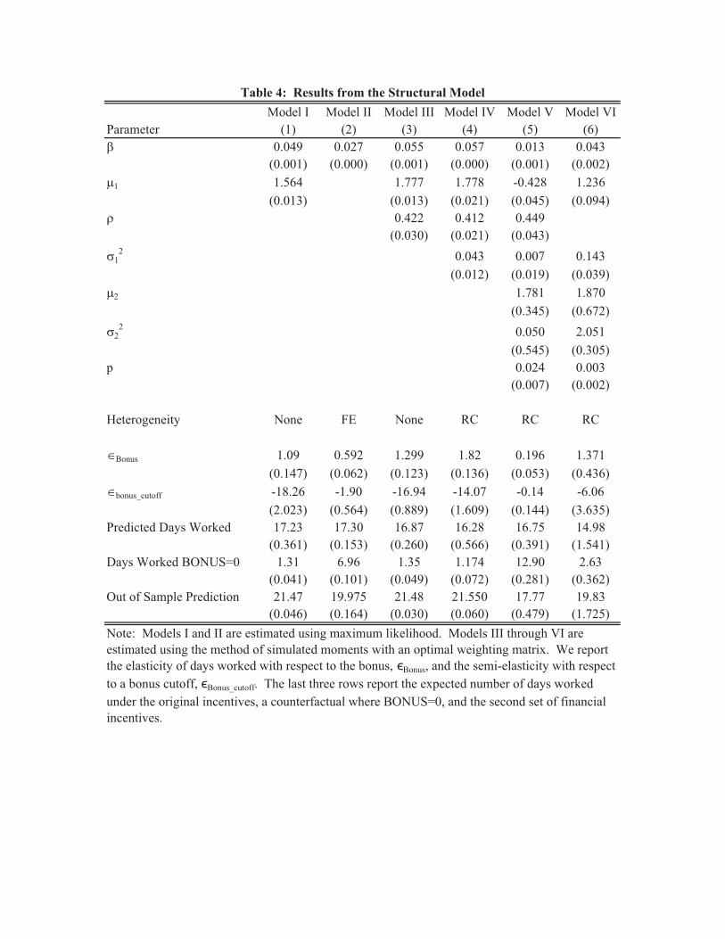
Model I Model II Model III Model IV Model V Model VIParameter (1) (2) (3) (4) (5) (6)� 0.049 0.027 0.055 0.057 0.013 0.043
(0.001) (0.000) (0.001) (0.000) (0.001) (0.002)�1 1.564 1.777 1.778 -0.428 1.236
(0.013) (0.013) (0.021) (0.045) (0.094)� 0.422 0.412 0.449
(0.030) (0.021) (0.043)�1
2 0.043 0.007 0.143(0.012) (0.019) (0.039)
�2 1.781 1.870(0.345) (0.672)
�22 0.050 2.051
(0.545) (0.305)p 0.024 0.003
(0.007) (0.002)
Heterogeneity None FE None RC RC RC
�Bonus 1.09 0.592 1.299 1.82 0.196 1.371(0.147) (0.062) (0.123) (0.136) (0.053) (0.436)
�bonus_cutoff -18.26 -1.90 -16.94 -14.07 -0.14 -6.06(2.023) (0.564) (0.889) (1.609) (0.144) (3.635)
Predicted Days Worked 17.23 17.30 16.87 16.28 16.75 14.98(0.361) (0.153) (0.260) (0.566) (0.391) (1.541)
Days Worked BONUS=0 1.31 6.96 1.35 1.174 12.90 2.63(0.041) (0.101) (0.049) (0.072) (0.281) (0.362)
Out of Sample Prediction 21.47 19.975 21.48 21.550 17.77 19.83(0.046) (0.164) (0.030) (0.060) (0.479) (1.725)
Table 4: Results from the Structural Model
Note: Models I and II are estimated using maximum likelihood. Models III through VI are estimated using the method of simulated moments with an optimal weighting matrix. We report the elasticity of days worked with respect to the bonus, �Bonus, and the semi-elasticity with respect to a bonus cutoff, �Bonus_cutoff. The last three rows report the expected number of days worked under the original incentives, a counterfactual where BONUS=0, and the second set of financial incentives.

Figure 4A: Predicted Fit From Model V
Figure 4B: CounterFactual Fit From Model V
Model�V����Predicted�Fit
0
0.02
0.04
0.06
0.08
0.1
0.12
0.14
0.16
1 2 3 4 5 6 7 8 9 10 11 12 13 14 15 16 17 18 19 20 21 22 23 24 25 26 27 28
Days
Fraction
Actual Mean 2.5�Percentile 97.5�Percentile
Model�V����Counterfactual�Fit
0
0.02
0.04
0.06
0.08
0.1
0.12
0.14
0.16
1 2 3 4 5 6 7 8 9 10 11 12 13 14 15 16 17 18 19 20 21 22 23 24 25 26 27 28
Days�
Fraction
Actual Mean 2.5�Percentile 97.5�Percentile

Trea
tmen
t C
ontro
lD
iffU
ntil
Mid
-Tes
tM
id to
Pos
t Tes
tA
fter P
ost T
est
(1)
(2)
(3)
(4)
(5)
(6)
0.72
0.73
-0.0
10.
010.
04-0
.01
(0.0
1)(0
.89)
(0.0
3)(0
.02)
1239
867
2106
643
480
983
0.55
0.57
-0.0
2-0
.02
0.05
-0.0
4(0
.02)
(0.0
4)(0
.05)
(0.0
3)12
3986
721
0664
348
098
3
Bla
ckbo
ards
Util
ized
0.92
0.93
-0.0
1-2
5676
6.00
0.01
-0.0
1(0
.01)
(0.0
2)(0
.02)
(0.0
2)99
070
816
9861
347
261
3N
otes
: (1
) Tea
cher
Per
form
ance
Mea
sure
s fro
m R
ando
m C
heck
s onl
y in
clud
es sc
hool
s tha
t wer
e op
en d
urin
g th
e ra
ndom
che
ck. (
2)
Stan
dard
err
ors a
re c
lust
ered
by
scho
ol.
Tab
le 6
: T
each
er P
erfo
rman
ceSe
pt 2
003-
Feb
2006
Perc
ent o
f Tea
cher
s Int
erac
ting
with
St
uden
ts
Perc
ent o
f Chi
ldre
n Si
tting
With
in
Cla
ssro
om
Diff
eren
ce B
etw
een
Trea
tmen
t and
Con
trol S
choo
ls
Expe
cted
Day
s W
orke
dBo
nus
Cuto
ffBo
nus
Expe
cted
Cos
t(1
)(2
)(3
)(4
)14
00
500
1521
2552
116
2275
664
1721
7567
218
2075
755
1920
100
921
2020
125
1112
2116
225
2642
2211
275
4604
Tabl
e 5:
Cou
nter
fact
ual C
ost-M
inim
izin
g P
olic
ies
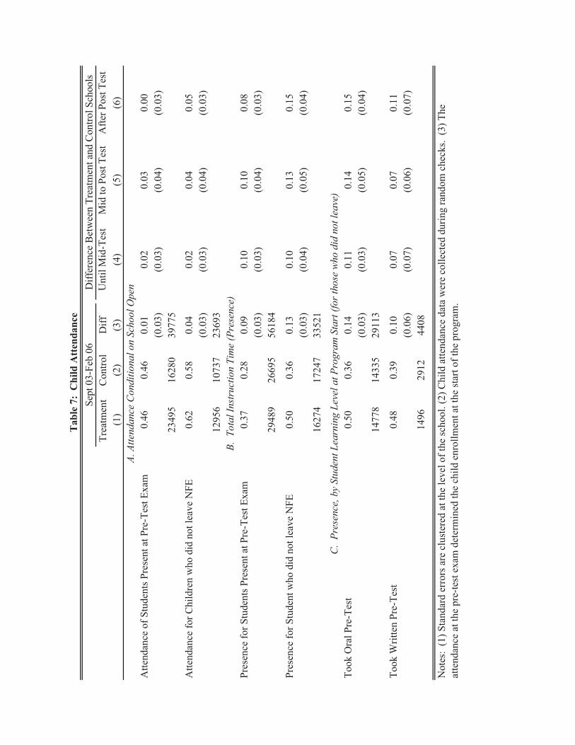
Trea
tmen
t C
ontro
lD
iffU
ntil
Mid
-Tes
tM
id to
Pos
t Tes
tA
fter P
ost T
est
(1)
(2)
(3)
(4)
(5)
(6)
Atte
ndan
ce o
f Stu
dent
s Pre
sent
at P
re-T
est E
xam
0.46
0.46
0.01
0.02
0.03
0.00
(0.0
3)(0
.03)
(0.0
4)(0
.03)
2349
516
280
3977
5
Atte
ndan
ce fo
r Chi
ldre
n w
ho d
id n
ot le
ave
NFE
0.62
0.58
0.04
0.02
0.04
0.05
(0.0
3)(0
.03)
(0.0
4)(0
.03)
1295
610
737
2369
3
Pres
ence
for S
tude
nts P
rese
nt a
t Pre
-Tes
t Exa
m0.
370.
280.
090.
100.
100.
08(0
.03)
(0.0
3)(0
.04)
(0.0
3)29
489
2669
556
184
Pres
ence
for S
tude
nt w
ho d
id n
ot le
ave
NFE
0.50
0.36
0.13
0.10
0.13
0.15
(0.0
3)(0
.04)
(0.0
5)(0
.04)
1627
417
247
3352
1
Took
Ora
l Pre
-Tes
t0.
500.
360.
140.
110.
140.
15(0
.03)
(0.0
3)(0
.05)
(0.0
4)14
778
1433
529
113
Took
Writ
ten
Pre-
Test
0.48
0.39
0.10
0.07
0.07
0.11
(0.0
6)(0
.07)
(0.0
6)(0
.07)
1496
2912
4408
Tab
le 7
: C
hild
Att
enda
nce
Sept
03-
Feb
06
D
iffer
ence
Bet
wee
n Tr
eatm
ent a
nd C
ontro
l Sch
ools
Not
es:
(1) S
tand
ard
erro
rs a
re c
lust
ered
at t
he le
vel o
f the
scho
ol. (
2) C
hild
atte
ndan
ce d
ata
wer
e co
llect
ed d
urin
g ra
ndom
che
cks.
(3) T
he
atte
ndan
ce a
t the
pre
-test
exa
m d
eter
min
ed th
e ch
ild e
nrol
lmen
t at t
he st
art o
f the
pro
gram
.
A. A
ttend
ance
Con
ditio
nal o
n Sc
hool
Ope
n
B. T
otal
Inst
ruct
ion
Tim
e (P
rese
nce)
C.
Pres
ence
, by
Stud
ent L
earn
ing
Leve
l at P
rogr
am S
tart
(for
thos
e w
ho d
id n
ot le
ave)

Trea
tmen
tC
ontro
lD
iffer
ence
Trea
tmen
tC
ontro
lD
iffer
ence
Perc
ent A
ttriti
on0.
110.
22-0
.10
0.24
0.21
0.03
(0.0
5)(0
.04)
Diff
eren
ce in
Per
cent
Writ
ten
of P
re-T
est a
ttrite
rs-s
taye
rs0.
010.
030.
020.
06-0
.03
0.10
(0.0
6)(0
.06)
Diff
eren
ce in
Ver
bal T
est o
f Pre
-Tes
t attr
iters
-sta
yers
0.05
0.08
-0.0
30.
020.
12-0
.10
(0.1
4)(0
.14)
Diff
eren
ce in
Writ
ten
Test
of P
re-T
est a
ttrite
rs-s
taye
rs-0
.41
-0.2
3-0
.18
-0.1
9-0
.13
-0.0
6(0
.34)
(0.2
9)
Took
Writ
ten
0.36
0.33
0.03
0.61
0.57
0.04
(0.0
4)(0
.05)
Mat
h 0.
140.
000.
14-0
.08
-0.2
40.
16(0
.10)
(0.1
5)
Lang
uage
0.14
0.00
0.14
1.71
1.60
0.11
(0.1
0)(0
.11)
Tota
l0.
140.
000.
140.
350.
240.
12(0
.10)
(0.1
1)
Not
es:
(1) T
est S
core
s in
Pane
l B a
re n
orm
aliz
ed b
y th
e m
ean
of th
e m
id-te
st c
ontro
l. (2
) Sta
ndar
d Er
rors
are
clu
ster
ed b
y sc
hool
.
B. E
xam
Sco
re M
eans
Mid
Tes
tPo
st T
est
Tab
le 8
: D
escr
iptiv
e St
atis
tics f
or M
id T
est a
nd P
ost T
est
A. A
ttriti
on P
roce
ss

Math Lang Total Math Lang Total(1) (2) (3) (4) (5) (6) (7) (8)
0.04 0.15 0.16 0.17 0.06 0.21 0.16 0.17(0.03) (0.07) (0.06) (0.06) (0.04) (0.12) (0.08) (0.09)1893 1893 1893 1893 1760 1760 1760 1760
0.02 0.13 0.13 0.14 0.05 0.17 0.13 0.15(0.03) (0.07) (0.05) (0.06) (0.04) (0.10) (0.07) (0.07)1893 1893 1893 1893 1760 1760 1760 1760
0.14 0.13 0.15 0.2 0.13 0.16(0.08) (0.06) (0.07) (0.14) (0.09) (0.10)1550 1550 1550 1454 1454 1454
0.19 0.28 0.25 0.28 0.28 0.25(0.12) (0.11) (0.11) (0.18) (0.11) (0.12)343 343 343 306 306 306
0.07 0.18 0.18 0.2 0.07 0.22 0.17 0.18(0.03) (0.07) (0.07) (0.07) (0.05) (0.12) (0.09) (0.09)891 891 891 891 821 821 821 821
0.02 0.12 0.14 0.14 0.05 0.19 0.16 0.16(0.04) (0.09) (0.07) (0.07) (0.04) (0.15) (0.10) (0.10)988 988 988 988 929 929 929 929
B. With Controls
A. All Children
Table 9: Estimation of Treatment Effects for the Mid- and Post-Test Mid-Test Post-Test
TookWritten
TookWritten
C. Took Pre-Test Oral
D. Took Pre-Test Written
E. Girls
Notes: (1) The table presents the coefficient estimate of being in a treated school on the sum of a child's score on the oral and written exams. All regressions include controls for the child's learning levels prior to the program. (2) The mid and post test scores are normalized by mid test control group. (3) Controls in Row B include Block, Teacher Test Scores, and Infrastructure Index. (4) Standard errors are clustered by school.
F. Boys

Treatment Control Diff(1) (2) (3)
0.44 0.36 0.08(0.04)
0.26 0.16 0.10(0.03)
0.18 0.20 -0.02(0.03)
N 1136 1061 2197
Method: OLS OLS OLS 2SLSSample: Control Schools Treatment Schools Treatment Schools All SchoolsData: Random Check Random Check Photographs Random Check
(1) (2) (3) (4)
Took Written 0.02 0.28 0.36 0.26(0.10) (0.08) (0.11) (0.19)
Total Score 0.20 0.39 0.87 1.07(0.19) (0.21) (0.22) (0.43)
N 878 1015 1015 1893
Took Written 0.24 0.51 0.59 0.33(0.16) (0.15) (0.20) (0.22)
Total Score 0.58 1.17 0.98 0.97(0.35) (0.36) (0.53) (0.47)
N 883 877 877 1760
Notes: (1) Standard errors are clustered at the level of the school. (2) Dropouts are defined as those who were absent for the last five random checks in which a school was found open.
Table 10: Dropouts and Movement into Government Schools
Child Left NFE
Child Enrolled in Government School
Child Dropped Out of School
Table 11: Does the Random Check Predict Test Scores?
A. Mid-test (Sept 03-April 04)
B. Post-test (Sept 03 -Oct 04)
Notes: (1) The table presents the coefficient estimate of the teacher's attendance on the sum of a child's score on the oral and written exams. All regressions include controls for the child's learning levels prior to the program. (2) The mid and post test scores are normalized by the mid test control group. (3) Standard errors are clustered by school.
Recommended