1
Inflation Dynamics’ Micro Foundations: How Important is Imperfect Competition
Really?
Sara G. Castellanos and Jose A. Murillo♦
Abstract
This paper analyzes price formation and dynamics according to the industry structure. It divides manufacturing industries of Mexico into two groups: perfectly and imperfectly competitive. The results show that imperfectly competitive industries predominate. Then this classification is used to build consumer price sub indexes for the goods of both sectors. These sub indexes’ inflation dynamics indicate that the exchange rate pass-through in the perfectly competitive sector is significantly higher than in the imperfectly competitive sector, while wage pass-through only affects the imperfectly competitive sector. Also, that inflation inertia is lower in the former than in the latter; adding up in more volatility of the perfectly competitive inflation rate. For policy makers an interesting feature of the perfectly competitive price index is that the evidence suggests that its variations precede those of the imperfectly competitive price index. For economic theorists these features validate recent macroeconomic models with heterogeneous price setting behavior.
Keywords: Panzar-Rosse, Industry Structure, Inflation, Price Dynamics, Price Indexes
JEL: L16, E31, E32, E52, and E58
♦ Both authors are researchers at the Economic Studies Division of Banco de México. We thank the valuable suggestions of Manuel Ramos Francia, Daniel Garcés, Jose Luis Negrín and Alejandro Pérez-López, as well as the comments of the participants in Banco de México’s Seminar. Meney De la Peza, Armando Martínez, Mishelle Seguí and Fernando Solano provided a very efficient research assistance at various stages of this project. All remaining errors are responsibility of the authors. The views expressed in this paper do not necessarily represent those of Banco de México. Mailing address: Avenida 5 de Mayo # 18, 4th floor, Mexico City, D.F. 06059, Mexico. E-mail address: [email protected], [email protected].

2
Inflation Dynamics’ Micro Foundations: How Important is Imperfect Competition
Really?
1. Introduction
Macroeconomic models that rely on the assumption of imperfect competition to explain the
effectiveness of monetary policy, staggered prices, and inflation inertia are quite abundant
in the literature and increasingly accepted in the economics profession (Blanchard and
Fischer, 1989; Calvo, 1983, Mankiw, 2000). Calibrations of general equilibrium models
that incorporate product or labor markets that are monopolistically competitive reproduce
the dynamics of the United States key macroeconomic variables along the business cycle in
a quite accurate manner (Chari, Kehoe and McGrattan, 2000; Christiano, Eichenbaum and
Evans, 2001). Also, the merits of different stabilization strategies have been discussed with
models elaborated upon these building blocks (Calvo and Vegh, 1999). However, with few
exceptions like Hall (1988) or Basu and Fernald (1997) for the case of the United States,
empirical evidence regarding the extent of imperfectly competitive markets is lacking.
Evidence on whether inflation dynamics are substantially affected by this feature, based on
equilibrium error correction models that produce estimates of the price markups and the
labor cost push, is even more scant and mostly analyzed with aggregate data (De Brouwer
and Ericsson, 1995; Mehra, 2000; Bertocco et al, 2002, Faruquee, 2004).1 More recently,
as the international flows of trade have deepened competition in several industries the
question about the role of this process, in view of imperfectly competitive domestic
markets, as a crucial factor behind several successful disinflation stories observed in the
past 20 years has been raised by financial authorities (Rogoff, 2003). All these
developments suggest that it is a good time to assess this fruitful micro foundation with the
data and ask: is imperfect competition pervasive? If so, how does it affect price formation
and dynamics?
In this paper we use the data of the Mexican economy to provide an answer to these two
questions. First, we determine whether monopolistic competition is a common industry
structure in the manufacturing sector. To this end, we use the method proposed by Panzar
and Rosse (1987). Second, we build consumer price indexes of goods manufactured by 1 Morisset and Revoredo (1995) constitutes an interesting exception within this literature because it estimates price adjustment in the industry, agriculture, services and commerce sectors of Argentina.
3
perfectly and imperfectly competitive industries and examine their respective dynamics.
We do so by estimating error correction models that relate these prices to changes on labor
and imported input costs.
Our estimations of the Panzar-Rosse statistic show that imperfect competition is a
widespread market structure in the Mexican manufacturing sector. In the sample of 71
industries that we examine, which account for 47 percent of this sector’s sales during the
period 1994-2003 on average, this statistic suggests perfect competition in 12 industries and
69 imperfect competition industries. This group is divided into 27 monopolistically
competitive industries and 29 industries with monopolies or very collusive oligopolies.
The remaining 3 industries could be classified in either category (monopoly or
monopolistic competition). The 71 classified industries have a weight of 69.7 per cent in
the core merchandise price index, of which imperfect competitive industries account for
almost half of the referred price index.
One of the main findings of the paper is that price adjustment to labor and foreign input
cost shocks does differ across perfectly and imperfectly competitive industries in the
theoretically predicted way: in the perfectly competitive sectors prices respond to changes
on the exchange rate only, while prices of imperfectly competitive sectors respond to
changes on the exchange rate and on wages. The adjustment to changes in the relevant
variables is estimated to be faster in the former case than in the latter. In turn, this suggests
that even though in the long run industries in which firms enjoy market power do not
produce higher inflation, as cost push advocates assure, they do slow down prices’ speed of
convergence to a given target. This higher inertia of imperfectly competitive industries
with respect to perfectly competitive ones, together with the exchange rate pass-through in
the former being lower than in the latter, also implies that the inflation rate of perfectly
competitive industries is more volatile than the inflation of imperfectly competitive
industries.
Another interesting feature that the perfectly competitive manufactures price index exhibits
is that its variations precede those of the imperfectly competitive price index. Hence,
monitoring the evolution of these indexes might prove to be useful in order to identify
inflationary pressures.

4
Because of the connection between imperfect competition and staggered prices, these
findings relate very closely with recent contributions on the relevance of heterogeneous
price setting behavior. For the United States, Ohanian, Stockman and Kilian (1995)
explore the implications of monetary and real shocks in a business cycle model in which
the degree of price stickiness differs across sectors. Nominal prices in the sticky-price
sector are set one period in advance and output is determined by the quantity demanded (in
accordance with monopolistic competition models), but in the flexible price sector trade
occurs in a Walrasian fashion (in accordance with perfect competition). Following the
work of Chari, Kehow and McGrattan (2000), Bils and Klenow (2002) sketch a general
equilibrium sticky price model in which monopolistically competitive firms set price that
are staggered with different duration periods across goods. Their empirical analysis linking
the frequency of price changes with the degree of competition is the closest one to our
work. They find a significant negative correlation between the frequency of price changes
of the entry level items of the United States’ consumer price index on one hand, and the
four-firm concentration ratios, the wholesale markup, or the rate of product substitution in
the other. Therefore, our findings are complementary to this research, providing evidence
of its relevance for successful future modeling, as we will discuss later.
The rest of this paper is structured as follows. Section 2 is devoted to the classification of
the manufacturing industries by their market structure. Section 3 delves on price formation
and dynamics in perfectly competitive and imperfectly competitive industries. In section 4
we conclude with some policy implications of the different industry structures.
2. Classifying Perfectly and Imperfectly Competitive Industries
2.1 The Panzar-Rosse Statistic
Most econometric studies of market power focus on single market or industries (Bresnahan,
1989). The statistic proposed by Panzar and Rosse (1987) stands in the tradition of the
New Empirical Industrial Organization. It is based on the comparative statics of a reduced
form revenue equation. Although it is less powerful than structural models favored in
single industry studies, it offers the advantage of less stringent data requirements and
reduces the risk of model misspecifications. It is also regarded as a more powerful
5
indicator of market structure and behavior than industry concentration ratios or markups
measured with accounting data. These characteristics make it specially attractive for an
analysis that comprises several industries. Moreover, in the analysis of Mexico’s data this
method to determine market power is preferable to the method based on the cycle
properties of the Solow residual proposed by Hall (1988), as well as its extensions (Roeger,
1995).2 The reason is twofold. On one hand, those methods crucially assume that price
markups are constant during the analysis period, which is usually a long time series because
the value added data required for estimations is reported in a quarterly basis by most
countries. On the other hand, the effects on Mexican manufactures’ trade on production
after the adhering to the GATT in 1984 and to the NAFTA in 1994 raise serious doubts on
the validity of this assumption.3
For the sake of completeness in the rest of this section we describe how the Panzar-Rosse
statistic is built. We also explain the estimation method, the data and the industry structure
classification.
Let y be a vector of decision variables which affect the firm’s revenues so that R=R(y, z)
where z is a vector of exogenous variables that shift the firm’s revenue function. The
firm’s cost function also depends on y, so that C=C(y, w, t), where w is a vector of factor
prices also taken as given by the firm and t is a vector of exogenous variables that shift the
firm’s cost curve. Then the firm’s profit function is given by
( )twzyCR ,,,ππ =−=
Let y0 be the argument that maximizes this profit function and y1 be the output quantity that
maximizes ( )( )twhzy ,1,, +π , where the scalar h is greater or equal to zero. Define R0 as
( ) ( )twzRzyR ,,, *0 ≡ and ( ) ( )( )twhzRzyRR ,1,, *11 +≡= , where R* is the firm’s reduced
form revenue function. It follows by definition that
( )( ) ( )( )twhyCRtwhyCR ,1,,1, 0011 +−≥+−
2 Hall’s method proposes that a pro-cyclical Solow residual is an indication of market power. It is used to examine the Mexican manufacturing sector by Castañeda (1988). 3 In fact, Castañeda (2003) reports that pooled estimations a la Hall of Mexican manufacturing markups indicate a significant reduction in those sectors that experienced a strong liberalization process after the implementations of both GATT and NAFTA.

6
Using the fact that the cost function is linearly homogeneous in w, equation (2) can be
rewritten as
( ) ( ) ( ) ( )twyChRtwyChR ,,1,,1 0011 +−≥+− (1)
Similarly, it must also be the case that
( ) ( )twyCRtwyCR ,,,, 1100 −≥− (2)
Multiplying both sides of (2) by (1+h) and adding the result to (1) yields
( ) 001 ≥−− RRh (3)
Dividing both sides of (3) by –h2 yields
( ) ( )( ) ( )[ ] 0,,,1,/ **01 ≤−+=− htwzRtwhzRhRR (4)
This nonparametric result simply states that a proportional cost increase always results in a
decrease in the firm’s revenue. Assuming that the reduced form revenue function is
differential, taking the limit of (4) as 0→h and then dividing the result by R* yields
( ) 0*** ≤∂∂≡ ∑ RwRw iiψ
where the wi are the components of the vector w, so that wi denotes the price of the ith input
factor. This expression describes a restriction imposed on a profit-maximizing monopoly.
The sum of the factor price elasticities of the reduced-form revenue equation cannot be
positive. Intuitively, the question that the test statistic *ψ tries to answer is what is the
percentage change in the firm’s equilibrium revenue resulting from a one percent increase
in all factor prices. An increase in factor prices shifts the average and marginal cost curves
up. Consequently, the price charged by the monopolist goes up and the quantity decreases.
Since the monopolist operates on the elastic portion of the demand curve, total revenue is
lower. Hence *ψ is non-positive for the monopolist case.4 Panzar and Rosse cite two
models of equilibrium consistent with a positive value for *ψ :
1* =ψ For firms observed in long-run competitive equilibrium the sum of
elasticities of reduced form revenues with respect to factor prices equals
4 This case also is identified with a cartel or with an oligopoly with strong collusion.

7
unity. Because firms in a competitive industry are operating at the
minimum average cost, a proportional increase in input cost will foster
some firms to exit and revenues will go up for the surviving firms so that
the equilibrium is reestablished at the minimum average cost.
10 * ≤<ψ In a symmetric Chamberlinian equilibrium of monopolistic competition,
the sum of the elasticities of firm’s reduced form revenues with respect
to factor prices is positive and less than or equal to unity. This implies
that a proportional increase of input costs increases the average and
marginal cost curves inducing some firms to exit the industry until the
equilibrium is reestablished.
It should be noted that in the competitive and monopolistically competitive model, the
revenue function facing the firm depends on the action of potential or actual rivals, so the
firm no longer acts in isolation. Also, the results of the models hinge upon the assumption
that the observed firms are in a long-run equilibrium.
2.2 Estimation Method and Data
Applying the Panzar-Rosse test on industry structure requires a reduced form revenue
equation. As Shaffer and Disalvo (1994) and Fischer and Kamerschen (2003), we estimate
a log linear revenue equation given by
∑=
++=6
1)ln()ln()ln(
iii wcybaR (5)
in which the vector of input prices includes the industry wage, the exchange rate, the price
of gas, the price of electricity, and a domestic interest rate. This input choice obeys both to
their common usage in the sector examined and to the need of preserving uniformity in the
estimations. All variables are expressed in real terms and revenues, volumes and wages are
calculated per hours worked. To take into account that output quantity is endogenous,
equation (5) is estimated through two stage least squares (using a lag of output as
instrumental variable).

8
The Monthly Industrial Survey (MIS) contains information about sales, volumes of output,
remunerations, and employment of 205 manufactures (equivalent to the 6 digit aggregation
level according to the Standard Industrial Classification).5 Mexico’s Consumer Price Index
(CPI) contains 315 generic products and services, while the Core Merchandise Price Index
has 191 generics. From these we found a reasonable match with 71 manufacturing
industries, which we considered for our analysis.6 For the period of January 1994 to
December 2003, this sample covers an average of 47 percent of the manufacturing sector
sales.
2.3 Results
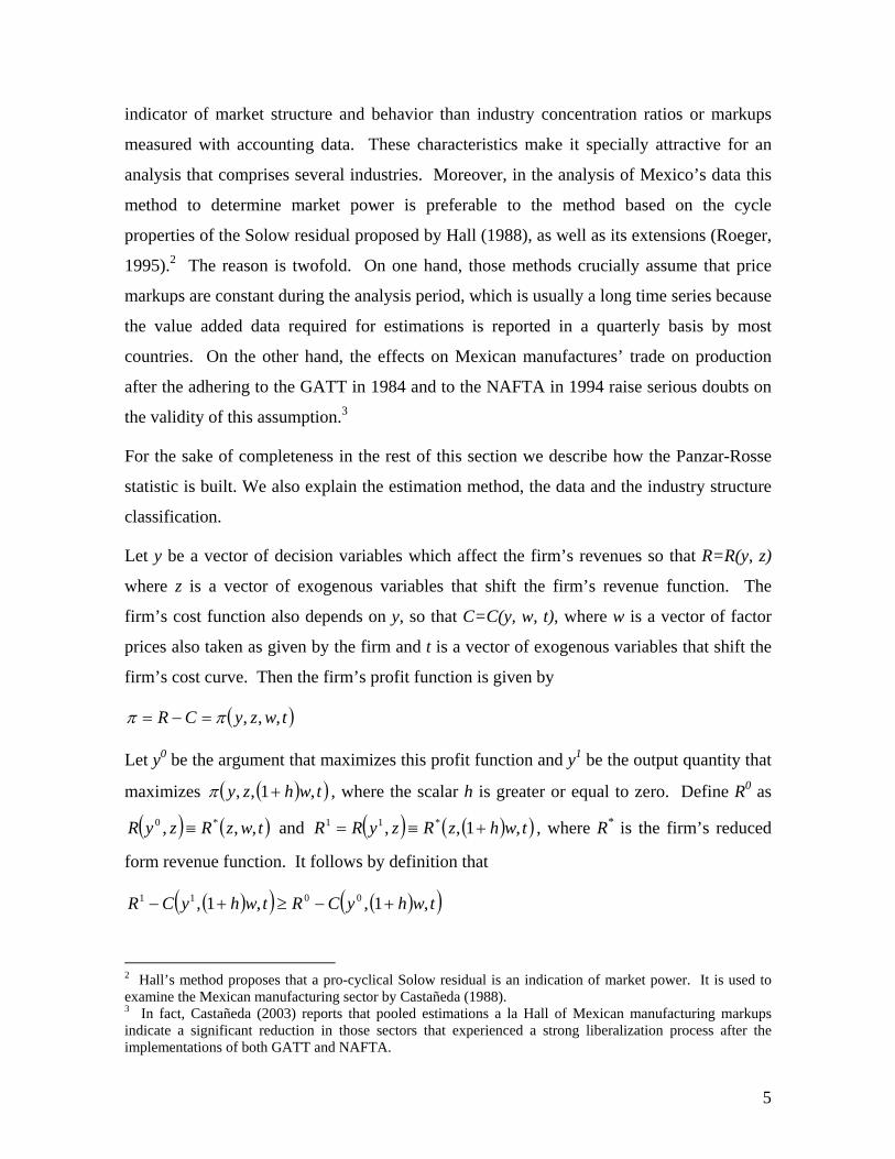
Table 1 presents the estimations of the Panzar-Rosse statistic for the 71 manufactures of our
sample. They take equation (5) as the initial specification, but input prices that are not
significant are excluded to obtain the most parsimonious revenue equation. The value of
the Panzar-Rosse statistics obtained suggest perfect competition in 12 industries; that is, the
statistic does not reject the hypothesis of being equal to one. Other 56 industries do reject
this hypothesis, which is consistent with imperfect competition. This group is divided into
43 monopolistically competitive industries, for which the hypothesis of being less than or
equal to zero is rejected, and 13 industries with monopolies, for which this hypothesis is not
rejected. There were 3 industries (knit underwear, shirts, and matches) in which none of
the input prices considered resulted statistically significant from zero under any
specification. Assuming that our input price list is complete, this result would be consistent
with a monopoly or cartel. On the other hand, the present estimations do not show any
industry with a statistic that is significantly larger than one, which in principle that may be
consistent with either competitive or monopoly models not proposed in Panzar and Rosse
(1987) and would require further scrutiny (probably with a structural model) to provide a
definite classification.
5 The Monthly Industrial Survey is produced by Mexico’s National Institute of Statistics, Geography and Information (INEGI). It is available at INEGI’s website (http//www.inegi.gob.mx). 6 Price data is produced by Banco de México (http://www.banxico.org.mx). This is also the source of the exchange rate and interest rate data that we used. The exchange rate that we employ is the end of month fix peso-U.S. dollar exchange rate that Banco de México publishes to settle transactions in U. S. dollars, the interest rate is the ex post real interest rate of 28 day Treasury Bonds (CETES). The series of Consumer Price Index of the United States was extracted from the Federal Reserve Bank’s website.
9
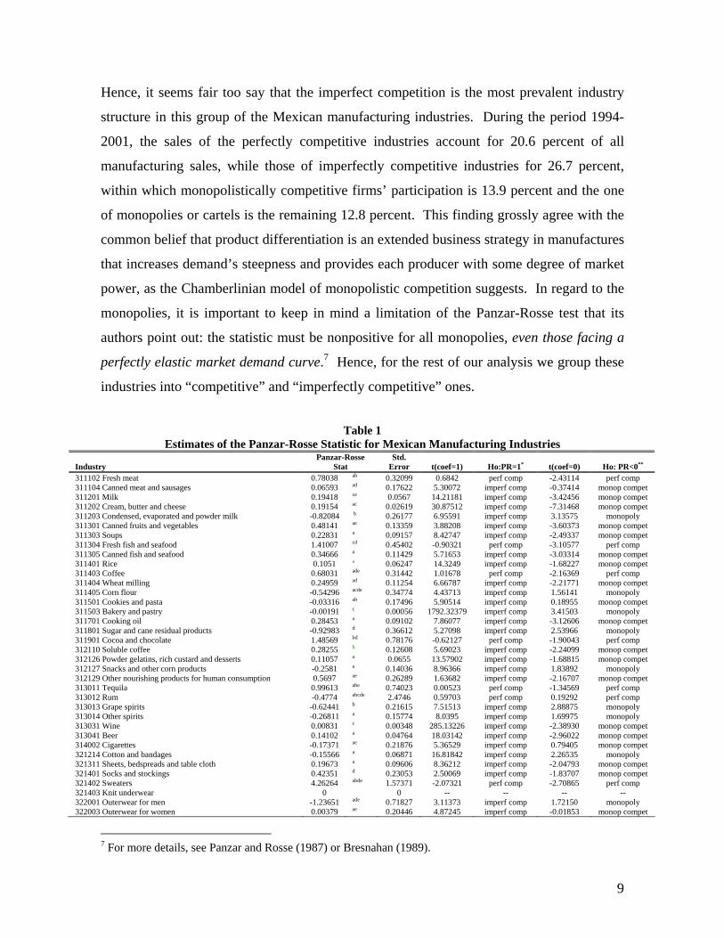
Hence, it seems fair too say that the imperfect competition is the most prevalent industry
structure in this group of the Mexican manufacturing industries. During the period 1994-
2001, the sales of the perfectly competitive industries account for 20.6 percent of all
manufacturing sales, while those of imperfectly competitive industries for 26.7 percent,
within which monopolistically competitive firms’ participation is 13.9 percent and the one
of monopolies or cartels is the remaining 12.8 percent. This finding grossly agree with the
common belief that product differentiation is an extended business strategy in manufactures
that increases demand’s steepness and provides each producer with some degree of market
power, as the Chamberlinian model of monopolistic competition suggests. In regard to the
monopolies, it is important to keep in mind a limitation of the Panzar-Rosse test that its
authors point out: the statistic must be nonpositive for all monopolies, even those facing a
perfectly elastic market demand curve.7 Hence, for the rest of our analysis we group these
industries into “competitive” and “imperfectly competitive” ones.
Table 1
Estimates of the Panzar-Rosse Statistic for Mexican Manufacturing Industries Industry
Panzar-Rosse Stat
Std. Error
t(coef=1)
Ho:PR=1*
t(coef=0)
Ho: PR<0**
311102 Fresh meat 0.78038 ab 0.32099 0.6842 perf comp -2.43114 perf comp 311104 Canned meat and sausages 0.06593 ad 0.17622 5.30072 imperf comp -0.37414 monop compet 311201 Milk 0.19418 ce 0.0567 14.21181 imperf comp -3.42456 monop compet 311202 Cream, butter and cheese 0.19154 ac 0.02619 30.87512 imperf comp -7.31468 monop compet 311203 Condensed, evaporated and powder milk -0.82084 b 0.26177 6.95591 imperf comp 3.13575 monopoly 311301 Canned fruits and vegetables 0.48141 ae 0.13359 3.88208 imperf comp -3.60373 monop compet 311303 Soups 0.22831 a 0.09157 8.42747 imperf comp -2.49337 monop compet 311304 Fresh fish and seafood 1.41007 cd 0.45402 -0.90321 perf comp -3.10577 perf comp 311305 Canned fish and seafood 0.34666 a 0.11429 5.71653 imperf comp -3.03314 monop compet 311401 Rice 0.1051 a 0.06247 14.3249 imperf comp -1.68227 monop compet 311403 Coffee 0.68031 ade 0.31442 1.01678 perf comp -2.16369 perf comp 311404 Wheat milling 0.24959 ad 0.11254 6.66787 imperf comp -2.21771 monop compet 311405 Corn flour -0.54296 acde 0.34774 4.43713 imperf comp 1.56141 monopoly 311501 Cookies and pasta -0.03316 ab 0.17496 5.90514 imperf comp 0.18955 monop compet 311503 Bakery and pastry -0.00191 c 0.00056 1792.32379 imperf comp 3.41503 monopoly 311701 Cooking oil 0.28453 a 0.09102 7.86077 imperf comp -3.12606 monop compet 311801 Sugar and cane residual products -0.92983 d 0.36612 5.27098 imperf comp 2.53966 monopoly 311901 Cocoa and chocolate 1.48569 bd 0.78176 -0.62127 perf comp -1.90043 perf comp 312110 Soluble coffee 0.28255 b 0.12608 5.69023 imperf comp -2.24099 monop compet 312126 Powder gelatins, rich custard and desserts 0.11057 a 0.0655 13.57902 imperf comp -1.68815 monop compet 312127 Snacks and other corn products -0.2581 a 0.14036 8.96366 imperf comp 1.83892 monopoly 312129 Other nourishing products for human consumption 0.5697 ae 0.26289 1.63682 imperf comp -2.16707 monop compet 313011 Tequila 0.99613 abe 0.74023 0.00523 perf comp -1.34569 perf comp 313012 Rum -0.4774 abcde 2.4746 0.59703 perf comp 0.19292 perf comp 313013 Grape spirits -0.62441 b 0.21615 7.51513 imperf comp 2.88875 monopoly 313014 Other spirits -0.26811 a 0.15774 8.0395 imperf comp 1.69975 monopoly 313031 Wine 0.00831 c 0.00348 285.13226 imperf comp -2.38930 monop compet 313041 Beer 0.14102 a 0.04764 18.03142 imperf comp -2.96022 monop compet 314002 Cigarettes -0.17371 ae 0.21876 5.36529 imperf comp 0.79405 monop compet 321214 Cotton and bandages -0.15566 a 0.06871 16.81842 imperf comp 2.26535 monopoly 321311 Sheets, bedspreads and table cloth 0.19673 a 0.09606 8.36212 imperf comp -2.04793 monop compet 321401 Socks and stockings 0.42351 d 0.23053 2.50069 imperf comp -1.83707 monop compet 321402 Sweaters 4.26264 abde 1.57371 -2.07321 perf comp -2.70865 perf comp 321403 Knit underwear 0 0 -- -- -- -- 322001 Outerwear for men -1.23651 ade 0.71827 3.11373 imperf comp 1.72150 monopoly 322003 Outerwear for women 0.00379 ae 0.20446 4.87245 imperf comp -0.01853 monop compet
7 For more details, see Panzar and Rosse (1987) or Bresnahan (1989).

10
322005 Shirts 0 0 -- -- -- -- 322006 Uniforms -0.03753 ad 0.22288 4.65507 imperf comp 0.16837 monop compet 322009 Outerwear for kids 0.54143 a 0.21464 2.13651 imperf comp -2.52257 monop compet 323003 Leather and rawhide products 0.11096 be 0.34703 2.56182 imperf comp -0.31974 monop compet 324001 Footwear, mainly of leather 0.58806 acde 0.17045 2.41681 imperf comp -3.45001 monop compet 332001 Furniture, mainly of wood -0.09807 ade 0.33929 3.23638 imperf comp 0.28903 monop compet 332003 Mattresses -0.24377 de 0.29794 4.17461 imperf comp 0.81820 monop compet 342001 Newspapers and magazines 0.48506 ae 0.15902 3.23832 imperf comp -3.05035 monop compet 342002 Books 0.24351 a 0.12013 6.29747 imperf comp -2.02712 monop compet 351222 Insecticide -0.12289 ad 0.39341 2.85426 imperf comp 0.31237 monop compet 352100 Pharmaceutical products 1.00731 ade 0.42081 -0.01737 perf comp -2.39373 perf comp 352221 Perfumes, cosmetics and similar 0.36721 d 0.12189 5.19154 imperf comp -3.01272 monop compet 352222 Soaps, detergents and toothpastes -0.16764 ab 0.19627 5.94928 imperf comp 0.85413 monop compet 352233 Matches 0 0 -- -- -- -- 352234 Films, plates and photography paper -0.78028 cd 0.15366 11.58618 imperf comp 5.07810 monopoly 352237 Cleaning and aromatic products 0.13632 abe 0.23754 3.63593 imperf comp -0.57389 monop compet 354002 Car lubricants 0.20635 bc 0.08622 9.20507 imperf comp -2.39330 monop compet 355001 Tires -0.45113 a 0.23229 6.24705 imperf comp 1.94209 monopoly 356005 Household plastic articles 0.02078 a 0.13063 7.49639 imperf comp -0.15906 monop compet 356011 Plastic toys 0.57632 a 0.31025 1.36561 imperf comp -1.85763 monop compet 362022 Glass and refractory products 1.00016 ae 0.40119 -0.00041 perf comp -2.49299 perf comp 383107 Batteries 0.62874 ab 0.32106 1.15635 perf comp -1.95830 perf comp 383109 Electric materials and accessories 0.10206 bcd 0.28396 3.16219 imperf comp -0.35942 monop compet 383110 Light bulbs, tubes and electric light bulbs -0.48812 e 0.25752 5.77876 imperf comp 1.89551 monopoly 383204 Music players and televisions 0.57578 b 0.32654 1.29915 imperf comp -1.76331 monop compet 383205 Music disks and tapes 0.21943 a 0.0718 10.87152 imperf comp -3.05606 monop compet 383301 Stoves and ovens 0.59494 ac 0.19246 2.10471 imperf comp -3.09128 monop compet 383302 Refrigerators and freezers 0.00681 c 0.00286 347.26993 imperf comp -2.38042 monop compet 383303 Washing and drying machines 0.0068 c 0.00366 271.14278 imperf comp -1.85749 monop compet 383304 Heating devices and house wares 0.10083 abe 0.33651 2.67205 imperf comp -0.29964 monop compet 384110 Cars and trucks 0.95281 abe 0.30292 0.15577 perf comp -3.14547 perf comp 384203 Motorcycles and bicycles 0.1838 bce 0.43343 1.88314 imperf comp -0.42406 monop compet 385002 Dental equipment -0.70722 e 0.22363 7.63408 imperf comp 3.16245 monopoly 385005 Eyeglasses 0.37131 ade 0.90546 0.69434 perf comp -0.41008 perf comp 390001 Jewelry, gold and silver work -0.01248 ace 0.35402 2.85996 imperf comp 0.03526 monop compet a=wage is statistically significant at the 10% level, b=exchange rate is statistically significant at the 10% level, c=interest rate is statistically significant at the 10% level, d=price of electricity is statistically significant at the 10% level, e=price of gas is statistically significant at the 10% level * Rejects the null hypothesis at the 10% level ** Rejects the null hypothesis at the 10% level
However, since some analysts may raise concerns regarding the fact that foreign
competition is an important reality in manufactures which may not be well accounted for in
the test we employ, in the next section we also distinguish imperfectly competitive
industries taking into account the share of imports to domestic sales according to a
threshold 30 percent.
3. Price Formation and Dynamics in Perfectly and Imperfectly Competitive Industries
3.1 Price Indexes
With the Panzar-Rosse industry classification we built a price index for goods produced in
perfectly and imperfectly competitive industries. The generics included in both indexes
have a weight of 25.8 percent in the CPI and 69.68 percent of the core merchandise price
index. The imperfectly competitive industries price index has a larger weight in the CPI
than perfectly competitive industries; the former accounts for 18.7 percent and the latter for
11
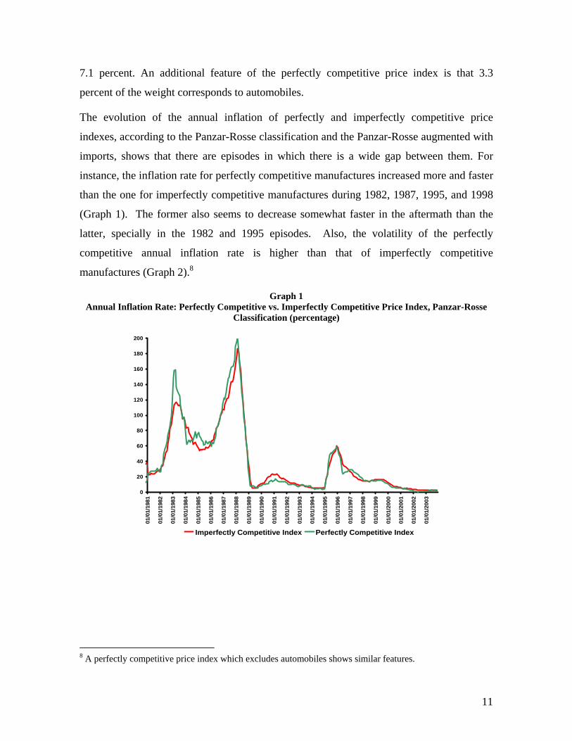
7.1 percent. An additional feature of the perfectly competitive price index is that 3.3
percent of the weight corresponds to automobiles.
The evolution of the annual inflation of perfectly and imperfectly competitive price
indexes, according to the Panzar-Rosse classification and the Panzar-Rosse augmented with
imports, shows that there are episodes in which there is a wide gap between them. For
instance, the inflation rate for perfectly competitive manufactures increased more and faster
than the one for imperfectly competitive manufactures during 1982, 1987, 1995, and 1998
(Graph 1). The former also seems to decrease somewhat faster in the aftermath than the
latter, specially in the 1982 and 1995 episodes. Also, the volatility of the perfectly
competitive annual inflation rate is higher than that of imperfectly competitive
manufactures (Graph 2).8
Graph 1 Annual Inflation Rate: Perfectly Competitive vs. Imperfectly Competitive Price Index, Panzar-Rosse
Classification (percentage)
0
20
40
60
80
100
120
140
160
180
200
01/0
1/19
81
01/0
1/19
82
01/0
1/19
83
01/0
1/19
84
01/0
1/19
85
01/0
1/19
86
01/0
1/19
87
01/0
1/19
88
01/0
1/19
89
01/0
1/19
90
01/0
1/19
91
01/0
1/19
92
01/0
1/19
93
01/0
1/19
94
01/0
1/19
95
01/0
1/19
96
01/0
1/19
97
01/0
1/19
98
01/0
1/19
99
01/0
1/20
00
01/0
1/20
01
01/0
1/20
02
01/0
1/20
03
Imperfectly Competitive Index Perfectly Competitive Index
8 A perfectly competitive price index which excludes automobiles shows similar features.

12
Graph 2 Rolling Variation Coefficient Gap of Perfectly and Imperfectly Competitive Annual Inflation
(24 month window)
-4
-2
0
2
4
6
8
10
12
Jan-
80
Jan-
81
Jan-
82
Jan-
83
Jan-
84
Jan-
85
Jan-
86
Jan-
87
Jan-
88
Jan-
89
Jan-
90
Jan-
91
Jan-
92
Jan-
93
Jan-
94
Jan-
95
Jan-
96
Jan-
97
Jan-
98
Jan-
99
Jan-
00
Jan-
01
Jan-
02
Jan-
03
An interesting feature of perfectly competitive inflation is that its variations precede those
of imperfectly competitive inflation. Graph 3 depicts the correlation coefficient of perfectly
and imperfectly competitive inflation first differences according to the Panzar-Rosse
classification in periods t and t-i, respectively; it is evident that it is skewed to the right.
Hence, the perfectly competitive price index might be for policy makers a useful statistic to
monitor future inflationary pressures.
Graph 3 Correlation Coefficient: First Difference of Perfectly Competitive Manufactures Inflation in t and
Imperfectly Competitive Manufactures Inflation in t-i, January 1990 - November 2003
0.30
0.35
0.40
0.45
0.50
0.55
0.60
0.65
0.70
0.75
t-4 t-3 t-2 t-1 0 t+1 t+2 t+3 t+4
13
3.2 Price Formation and Dynamics
Error correction type equations are increasingly popular choices to model price behavior.
Applying this technique for our analysis has the advantage of making our estimations
comparable to previous work about Mexico’s inflation dynamics (Garcés, 2001 and
Baillieu et al, 2003). For each price index we estimate the following equation:
tttttttt uecwcpcpcecwccp +∆+∆+∆++++=∆ −−−− 76151413121 (6)
where pt is the log price index, wt is the log nominal wage cost, and et is log foreign input
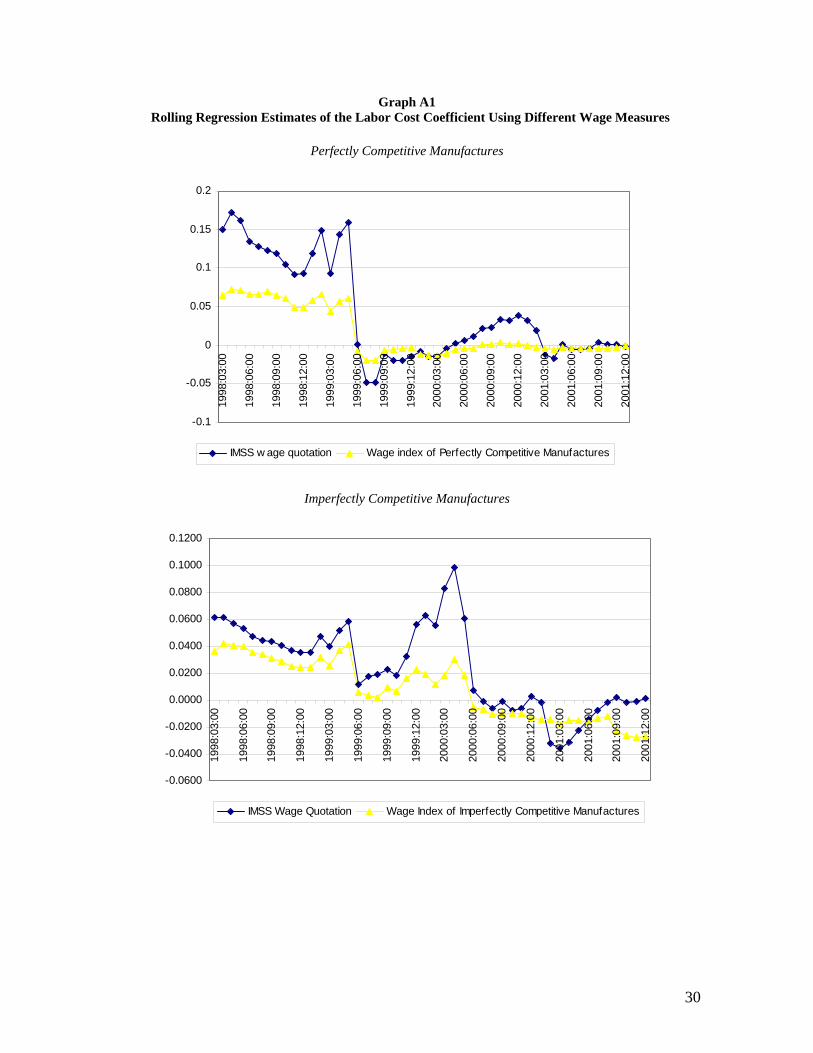
cost. To expand our sample period until 1985, in this section our wage measure is the
average wage quotation of the Mexican Social Security Institute (IMSS). However,
estimations with this variable are very similar to those that employ the wage indexes of
competitive and imperfectly competitive manufactures constructed with the MIS data of
Section 2 (see appendix).9 The cost of foreign inputs is measured through the real
exchange rate, constructed as the peso-dollar exchange rate times the consumer price index
of the United States.
Notice that in equation 6, pt-1, wt-1 and et-1 constitute the error correction term, which
depicts the long run relationship among the variables. This relationship can be derived
from a unit cost inflation model that represents the price as a Cobb Douglass function of the
wages and the exchange rate, ew EWP λλµ= , where λw>0 and λe>0 are the respective long
run elasticities and µ>0 is a price mark up over costs (De Brouwer and Ericsson, 1998). It
is straightforward to show that when linear homogeneity is imposed and this price equation
is expressed in logarithms λw=-c2/c4, λe=-c3/c4. In the appendix we verify through the
appropriate Johansen cointegration tests that this relationship satisfies the required
stationarity conditions, which support the existence of a stable long run mark up.10
9 These estimations are available from the authors upon petition. 10 Notice that we could have estimated the equation tttttt uecwcpcectccp +∆+∆+∆++=∆ − 761581 , where
tetwtt ewpect λλ −−= and satisfies stationarity, instead. But the specification we use has the advantage of suggesting a specific cointegration relationship at instances where there are more than one and the cointegration and exogeneity tests presented in the appendix indicate very similar results. In particular, the coefficient of the pt and of ectt has the expected sign and is statistically significant according to the applicable distribution of error correction tests for cointegration (Ericsson and MacKinnon, 1999), although in the former case that of the wt and et is not properly assessed. Still, we prefer equation 6 for illustration purposes.

14
In Table 2 we report the estimations of equation 6 with the CPI, the core merchandise price
index, the core services price index, and our industry structure price indexes. The first of
them divides manufactures between perfectly and imperfectly competitive ones taking the
baseline Panzar-Rosse threshold only and the second one combines the Panzar-Rosse index.
In general, the coefficients of the error correction term variables, c2, c3 and c4, have the
expected sign and are significant at conventional levels: inflation rises as a response to
either wage or exchange rate increases, but price disturbances have a transitory nature and
converge to the long term equilibrium level; that is a negative coefficient associated to the
lagged price level. For the CPI, the estimated coefficients largely coincide with the
previous results of Garcés (2001) or Baillieu et al (2003). Moreover, if we take this
equation as baseline, we appreciate a tendency in which the equations for price indexes of
manufactures produced in imperfectly competitive industries to show smaller coefficients
of lagged exchange rate and lagged price level and a larger coefficient associated to the
lagged wage than those of manufactures from perfectly competitive. In fact, the wage
coefficient of the perfectly competitive index is negative but not statistically significant. So
for this index we also examined a version of equation 6 without the wage variable. This
version yields a slightly lower coefficients for the exchange rate (0.044789) and the lagged
price (-0.049121), both statistically significant, that those reported in the table. Since
cointegration and exogeneity tests also resulted very similar across the two specifications,
we only report those of the baseline equation.11
On the other hand, the coefficients of c5, c6 and c7 that account for the short term effects
also have the expected signs, but their statistical significance varies across regressions.
Also, the adjusted-R2 and the F-statistic respectively suggest that equation (6) has good
data fit and overall statistical significance. Lastly, the recursive and rolling regression
estimations show that the coefficients are stable (in the appendix we present the
corresponding graphs for the error correction term coefficients).
11 The rest of the tests are available from the authors upon petition.

15
Table 2 Estimation Results of Price Error Correction Models of Perfectly and Imperfectly Competitive
Manufactures Dependent Variable c2 c3 c4 c5 c6 c7 Adj. R2 F-stat. Prob(F-stat)
Coeff.. 0.0318 0.0414 -0.0727 0.6321 0.0230 0.0247 0.9007 120.5421 0 Std. Error 0.0069 0.0059 0.0111 0.0828 0.0313 0.0284 t-Stat. 4.6250 6.9773 -6.5217 7.6318 0.7348 0.8676
CPI
Prob. 0.0000 0.0000 0.0000 0.0000 0.4633 0.3866
Coeff.. 0.0120 0.0303 -0.0432 0.7664 0.0719 0.0215 0.9195 151.5052 0 Std. Error 0.0051 0.0080 0.0119 0.0695 0.0263 0.0159 t-Stat. 2.3520 3.8010 -3.6210 11.0275 2.7360 1.3480
CORE MERCHANDISE PRICE INDEX
Prob. 0.0196 0.0002 0.0004 0.0000 0.0068 0.1791
Coeff.. 0.0177 0.0244 -0.0423 0.4903 0.0339 0.0103 0.8720 90.74364 0 Std. Error 0.0088 0.0044 0.0106 0.0919 0.0395 0.0259 t-Stat. 2.0199 5.4702 -4.0436 5.3328 0.8587 0.3962
CORE SERVICES PRICE INDEX
Prob. 0.0447 0 0.0001 0 0.3915 0.6924
Coeff. -0.00095 0.04738 -0.04999 0.62899 0.04959 0.06349 0.82071 61.31508 0 Std. Error 0.00373 0.01440 0.01693 0.09483 0.03570 0.04055 t-Stat. -0.25546 3.29045 -2.95284 6.63258 1.38881 1.56591
P of PERFECTLY COMPETITIVE MANUFACTURES
Prob. 0.79860 0.00120 0.00350 0.00000 0.16640 0.11890
Coeff. 0.01350 0.03604 -0.05237 0.68805 0.11909 0.01400 0.90994 134.13810 0 Std. Error 0.00401 0.00730 0.00990 0.07158 0.02639 0.00976 t-Stat. 3.36584 4.93997 -5.29289 9.61225 4.51227 1.43439
P of IMPERFECTLY COMPETITIVE MANUFACTURES
Prob. 0.00090 0.00000 0.00000 0.00000 0.00000 0.15300
Coeff. 0.002975 0.030111 -0.035658 0.746559 0.052167 0.048703 0.89874 117.9492 0 Std. Error 0.002833 0.010276 0.012602 0.077808 0.025739 0.02811 t-Stat. 1.050228 2.930103 -2.829653 9.594936 2.026749 1.73261
P of PERFECTLY COMPETITIVE MANUFACTURES OR WITH IMP. PEN. >30% Prob. 0.2948 0.0038 0.0051 0 0.044 0.0847
Coeff. 0.020218 0.052435 -0.075853 0.56548 0.149384 0.003489 0.865407 85.7224 0.0000 Std. Error 0.005234 0.007237 0.010074 0.074954 0.036979 0.011005 t-Stat. 3.862994 7.245489 -7.529308 7.544315 4.039721 0.317049
P of IMPERFECTLY COMPETITIVE MANUFACTURES WITH IMP. PEN < 30% Prob. 0.0001 0 0 0 0.0001 0.7515 Method: Least Squares Sample(adjusted): 1985:02 2003:10 Included observations: 225 after adjusting endpoints Newey-West HAC Standard Errors & Covariance (lag truncation=4)
One of the features in which inflation of perfectly and imperfectly competitive industries
differ is on the degree of inertia. Price formation in perfectly competitive industries relies
significantly less on past inflation than in imperfectly competitive industries. In the first
case, the lagged inflation coefficient is 0.30 and in the second 0.76. In the other three cases
the lagged inflation coefficient is somewhat larger for the perfectly competitive industries
and somewhat lower for the imperfectly competitive ones. Due to the core services
component and the fact that perfectly competitive manufactures have a low share in the
merchandise component, the CPI’s lagged inflation coefficient is closer to that of the
imperfectly competitive inflation ( 0.63).
Next, in Table 3 we show the estimations of the long run pass-through coefficients λw and
λe. As expected, given the values of c2, c3 and c4 obtained, the coefficients’ magnitudes in
the CPI equation coincide with the previous studies: if the exchange rate depreciates by 10

16
percent then prices increases by 5.7 percent, while if wages costs increase by 10 percent
prices increase by 4.4 percent. In the case of core merchandise inflation the exchange rate
pass-through is 0.70, while the wage pass-through is 0.28. In contrast, pass-through
coefficients for the inflation rate in the perfectly competitive industries differ significantly,
since wage variations have a nil effect and price dynamics depend only on the exchange
rate.12 However, the results for imperfectly competitive industries inflation are closer to
those of core services inflation (partly due to the weight they have on the index) with
exchange rate and wage pass-through coefficients of 0.69 and 0.26, respectively, using the
Panzar-Rosse classification. The pass-through coefficients are similar independently of the
threshold of import to domestic sales that we use and for different specifications of the
Panzar-Rosse revenue equation.
Table 3 Pass-Through Coefficients of Wage and Exchange Rate of Perfectly and Imperfectly Competitive
Manufactures
Dependent Variable λw λe
CPI 0.4370 0.5690
CORE INFLATION MERCHANDISE 0.2771 0.7013
CORE INFLATION SERVICES 0.4150 0.5723
P of PERFECTLY COMPETITIVE MANUFACTURES -0.0190 0.9478
P of IMPERFECTLY COMPETITIVE MANUFACTURES 0.2577 0.6881
P of PERFECTLY COMPETITIVE MANUFACTURES OR WITH IMP. PEN. >30% 0.0834 0.8444
P of IMPERFECTLY COMPETITIVE MANUFACTURES WITH IMP. PEN < 30% 0.2665 0.6913
In addition, Graph 4 and 5 displays the pass-through coefficient dynamics with a rolling
regression estimation. They provide an additional grasp of their stability through time,
specially after 1996. For both wages and the exchange rate periods in which the prices of
one sector show a higher pass-through than the other are observed. After 2002, it seems
that the exchange rate pass through has been higher for the perfectly competitive index and
lower for the imperfectly competitive index, while the wage pass through has had the
opposite pattern.
12 See note

17
Graph 4 Rolling Regression Estimates of the Exchange Rate Pass Through
-0.3
0
0.3
0.6
0.9
1.2
1.5
1993
:11:
00
1994
:04:
00
1994
:09:
00
1995
:02:
00
1995
:07:
00
1995
:12:
00
1996
:05:
00
1996
:10:
00
1997
:03:
00
1997
:08:
00
1998
:01:
00
1998
:06:
00
1998
:11:
00
1999
:04:
00
1999
:09:
00
2000
:02:
00
2000
:07:
00
2000
:12:
00
2001
:05:
00
2001
:10:
00
2002
:03:
00
2002
:08:
00
2003
:01:
00
2003
:06:
00
price index of perfectly competitive manufacturesprice index of imperfectly competitive manufactures
Graph 5 Rolling Regression Estimates of the Wage Pass-Through
-0.3
0
0.3
0.6
0.9
1.2
1.5
1993
:11:
00
1994
:04:
00
1994
:09:
00
1995
:02:
00
1995
:07:
00
1995
:12:
00
1996
:05:
00
1996
:10:
00
1997
:03:
00
1997
:08:
00
1998
:01:
00
1998
:06:
00
1998
:11:
00
1999
:04:
00
1999
:09:
00
2000
:02:
00
2000
:07:
00
2000
:12:
00
2001
:05:
00
2001
:10:
00
2002
:03:
00
2002
:08:
00
2003
:01:
00
2003
:06:
00
price index of perfectly competitive manufacturesprice index of imperfectly competitive manufactures
4. Some Policy Implications
The results in this paper show that the Mexican manufacturing industry is predominantly
characterized by an imperfectly competitive structure. Also, it finds that the inflation
18
dynamics of perfectly and imperfectly competitive industries have significant differences.
For instance, the evidence we find shows that in the long run perfectly competitive
manufactures prices are affected solely by exchange rate variations. This pattern is
consistent with the law of one price. On the other hand, in imperfectly competitive
manufactures wage variations also affect prices, which in principle is consistent with a cost
push.
The cost-push view of the wage-price dynamics implies that monetary policy and the
resulting inflation environment do not matter in determining the ability of firms to pass
forward higher wage costs in the form of higher product prices. Higher wage growth
should lead to higher future inflation irrespective of the monetary policy stance and the
inflation history. Thus, this view requires in addition to the existence of a long term
relationship between prices and wages, which is sustained for both the perfectly and the
imperfectly price indexes in the cointegration tests we perform, that this long term
relationship is in fact the long term price equation in which wages can be considered
exogenous (Mehra, 2000). To verify this possibility we check the weak exogeneity
properties of the variables included in the price relationship estimating a vector error
correction model with the key analysis variables (see appendix). The estimations do not
result supportive of the cost push view of inflation because the only weakly exogenous
variable of the system is the price level.13 Hence, this finding suggests that the central
bank’s policy does matter in determining the ability of firms to pass forward higher wage
costs in the form of higher product prices.
An additional feature is that perfectly competitive manufactures have a lower degree of
inflationary inertia than imperfectly competitive industries. This may imply different
employment responses, with less employment adjustment where prices vary more. The
classification of industries used to build the price indexes can be used to build output and
employment indexes with the MIS data. This variables can be put together in vector
autorregressions to obtain the impulse response functions of two sectors that differ on their
degree of price stickiness to innovations in future research. On the other hand, this feature
13 In fact, the perfectly competitive price index satisfies the weak exogeneity condition barely. But additional Granger causality tests do reject the hypothesis that this price index does not cause wages and do not reject the hypothesis that wages cause prices.

19
would also suggest that an inflationary bout could produce a significant relative price
misalignment between the goods produced in perfectly and imperfectly competitive
industries. Evidently, when inflation is trending downwards the effect would the opposite,
producing a reallocation of resources within the manufacturing industry. All this aspects
may be analyzed with a multi-sector theoretical model in the fashion of Ohanian, Stockman
and Kilian (1995) or Bils and Klenow (2002).
Another interesting finding of this study is the high degree of coincidence among industries
with high import penetration and industries with a Panzar-Rosse statistic value suggestive
of perfect competition in the manufacturing sector. Evidently the power of import
competition to discipline prices is well recognized among economists. But the present
results, together with the fact that data requirements to calculate import penetration ratios
are less than those to estimate indicators of an industry’s structure or competition level, beg
questioning whether the price formation processes described are solely explained by
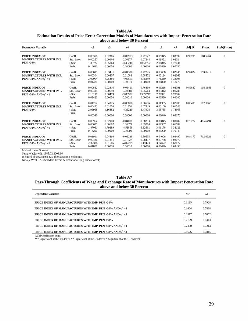
foreign competition.14 To address this issue we calculated the price indexes for
manufactures with an import penetration rate higher and lower than 30 percent of total sales
and, within these two groups, the price indexes for manufactures with a Panzar-Rosse
statistic equal or less than 1. Then we estimated the price equation for this six categories.
This exercise shows that among manufactures with a high import penetration rate, the
perfectly competitive ones again exhibit higher exchange rate coefficients and lower wage
coefficients. This pattern is also observed among manufactures with a low import
penetration rate. As a result, the wage pass-through was not significant for the price of
manufactures with a high import penetration rate, regardless of the degree of competition
suggested by the Panzar-Rosse statistic, and its significance in the price of manufactures
with a low import penetration rate can be traced to those where the Panzar-Rosse statistic is
compatible with imperfect competition (see appendix).
Therefore, these findings suggest an affirmative answer to the question regarding the role of
trade liberalization in a successful disinflation story, when a country’s domestic markets are
characterized by imperfect competition (Rogoff, 2003). However, higher exchange rate
pass-through and lower inertia of competitive manufactures inflation implies a higher
14 In 1993 when Mexico signed the NAFTA and passed a constitutional amendment to forbid monopolistic practices, passed a competition law and created a federal trade commission to perform its mandate.
20
volatility than in imperfectly competitive . The deepening of the globalization process and
its extension to the service sector makes foreseeable that industries will be subject to a
higher degree of competition. An implication of this process may be that, ceateris paribus,
CPI variations will depend even more on the evolution of the exchange rate. Also, this may
imply that for a certain level, inflation will be more volatile and therefore more costly to
keep within a target band during a short span of time. Also, higher industry competition
may translate into lower inflationary inertia and consequently a diminished role for
monetary policy stimulus over the coming years. All these aspects constitute an interesting
research agenda.
Finally, the evidence suggests that inflation of perfectly competitive manufactures precedes
that of imperfectly competitive manufactures. Hence, monitoring the evolution of the first
price index might prove to be useful in order to identify future inflationary pressures in the
economy.
5. References
Baillieu, J., Garcés, D., Kruger and M. Messmacher (2003) “Explicación y Predicción de la
Inflación en Mercados Emergentes: el Caso de México” (2003), Monetaria, vol. XXVI, no.
2, April-June.
Basu, S. and J. G. Fernald (1997), “Returns to Scale in U. S. Production: Estimates and
Implications,” Journal of Political Economy, vol. 105, no. 2, April, pages 249-283.
Bertocco, G., Fanelli, L. and P. Paruolo (2002), “On the Determinants of Inflation in Italy:
Evidence of Cost-Push Effects before the European Monetary Union,” Università
Dell’Insubria, Facoltà di Economia Working Paper No. 2002/41.
Bils, M. and P. J. Klenow (2002), “Some Evidence on the Importance of Sticky Prices.”
NBER Working Paper No. 9069.
Blanchard, O. and S. Fischer (1989), Lectures on Macroeconomics, MIT press, Cambridge,
Mass.
Calvo, G. (1983), “Staggered Prices in a Utility-Maximizing Framework,” Journal of
Monetary Economics, 12, pages 383-398.

21
Calvo, G. and C. Vegh (1999); “Inflation Stabilization and BOP Crises in Developing
Countries,” Handbook of Macroeconomics, vol 1C (North-Holland, 1999), edited by J.
Taylor and M. Woodford.
Castañeda, A. (1998), “Measuring the Degree of Collusive Conduct in the Mexican
Manufacturing Sector,” Estudios Económicos, vol. 13, no. 2, pages 157-169.
Castañeda, A. (2003), “Mexican Manufacturing Markups: Cyclical Behavior and the
Impact of Trade Liberalization.” Economía Mexicana, vol. XII, no. 2.
Chari, V. V., Kehoe, P. J. and E. R. McGrattan (2000), “Sticky Price Models of the
Business Cycle: Can the Contract Multiplier Solve the Persistence Problem?,”
Econometrica 68, pp 1151-1179.
Christiano, L. J., Eichenbaum, M. and C. L. Evans (2001), “Nominal Rigidities and the
Dynamic Effects of a Shock to Monetary Policy,” Northwestern University and Federal
Reserve Bank of Chicago mimeograph.
De Brouwer, G. and N. R. Ericsson (1995), “Modeling Inflation in Australia,” Economic
Analysis and Economic Research Departments, Reserve Bank of Australia, Research
Discussion Paper No. 9510.
Ericsson N. R. and J. G. MacKinnon (1999), “Distributions of Error CorrectionTests for
Cointegration,” Board of Governors of the Federal Reserve System International Finance
Discussion Papers No. 655.
Garcés, D. (2001), “Determinación del Nivel de Precios y la Dinámica Inflacionaria en
México,” Monetaria , vol. XXIV, no. 3, July-September.
Faruquee, H. (2004), “Exchange Rate Pass-Through in the Euro Area: The Role of
Asymmetric Pricing Behavior”, IMF Working Paper No. 0414.
Fischer, T. and D. R. Kamerschen (2003), “Measuring Competition in the U. S. Airline
Industry using the Rosse-Panzar Test and Cross-Sectional Regression Analyses,” Journal
of Applied Economics, vol. VI, no. 1, May, pages 73-93.
Hall, R. E. (1988), “The Relation between Price and Marginal Cost in U. S. Industry,”
Journal of Political Economy, 96, October, pages, 921-947.

22
Mankiw, N. G. (2000), “The Inexorable and Mysterious Tradeoff Between Inflation and
Unemployment,” Harvard Institute of Economic Research, Discussion Paper No. 1905,
September.
Mehra, Y. (2000), “Wage-Price Dynamics: Are They Consistent with Cost Push?,” Federal
Reserve Bank of Richmond, Economic Quarterly, vol. 86/3, summer.
Morisset, J. and C. Revoredo (1995), “In Search of Price Rigidities (Recent Sector
Evidence from Argentina),” World Bank, Policy Research Working Paper No. 1558.
Obstfeld, Maurice (2002), “Exchange Rates and Adjustment: Perspectives from the New
Open Economy Macroeconomics,” NBER Working Paper No. 9118.
Ohanian, L. E., Stockman, A. C. and L. Kilian (1995), “The Effects of Real and Monetary
Shocks in a Business Cycle Model with Some Sticky Prices, “ Journal of Money, Credit,
and Banking, Vol. 27, No. 4 (November 1995 Part 2).
Panzar, J. C. and J. N. Rosse (1987), “Testing for ‘Monopoly’ Equilibrium,” Journal of
Industrial Economics, vol. 35, no. 4, The Empirical Renaissance in Industrial Economics,
June, pages 443-456.
Roeger, W. (1995), “Can Imperfect Competition Explain the Difference between Primal
and Dual Productivity Measures? Estimates for U. S. Manufacturing,” Journal of Political
Economy, vol. 103, no. 2, April, pages 316-330.
Shaffer, S. and J. Di Salvo (1994), “Conduct in a Banking Duopoly,” Journal of Banking
and Finance, 18, pages 1063-1082.

23
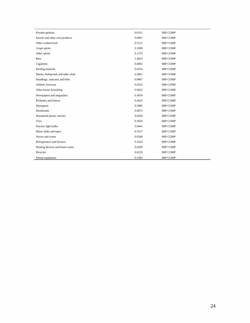
6. Appendix
Table A1 Industry Structure According to Panza-Rosse Classification and Share of Imports
Generic CPI Weight Panzar - Rose Imports > 30%
Fresh meat 1.2037 PERF COMP X
Sweaters for kids 0.0207 PERF COMP X
Glass and refractory products 0.0861 PERF COMP X
Eyeglasses 0.1888 PERF COMP X
Pharmaceutical products 1.2040 PERF COMP
Fresh fish and seafood 0.5611 PERF COMP
Coffee 0.0329 PERF COMP
Chocolate 0.0601 PERF COMP
Tequila 0.2771 PERF COMP
Rum 0.1224 PERF COMP
Batteries 0.0259 PERF COMP
Cars 3.3030 PERF COMP
Books 1.0238 IMP COMP X
Insecticide 0.0845 IMP COMP X
Furniture, mainly of wood 0.8228 IMP COMP X
Outerwear for men 0.7480 IMP COMP X
Outerwear for women 0.3932 IMP COMP X
Uniforms 0.2511 IMP COMP X
Outerwear for kids 0.5085 IMP COMP X
Socks 0.0635 IMP COMP X
Wine 0.0975 IMP COMP X
Films, plates and photography paper 0.0998 IMP COMP X
Car lubricants 0.1434 IMP COMP X
Tires 0.1322 IMP COMP X
Electric appliances 0.5778 IMP COMP X
Music players 0.3002 IMP COMP X
Washing and drying machines 0.1410 IMP COMP X
Watches, jewelry and imitation jewellery 0.0512 IMP COMP X
Canned meat and sausages 0.9186 IMP COMP
Milk 1.8649 IMP COMP
Milk derivatives 0.9688 IMP COMP
Condensed, evaporated and maternalized milk 0.0474 IMP COMP
Canned fruits and vegetables 0.3767 IMP COMP
Soups 0.0461 IMP COMP
Canned fish and seafood 0.1744 IMP COMP
Rice 0.1500 IMP COMP
Wheat milling 0.0304 IMP COMP
Corn flour 0.0362 IMP COMP
Generic cookies 0.0837 IMP COMP
Bakery 0.9841 IMP COMP
Cooking oil 0.3210 IMP COMP
Sugar 0.2073 IMP COMP
Soluble coffee 0.1183 IMP COMP
24
Powder gelatins 0.0311 IMP COMP
Snacks and other corn products 0.0967 IMP COMP
Other cooked food 0.5272 IMP COMP
Grape spirits 0.1009 IMP COMP
Other spirits 0.1375 IMP COMP
Beer 1.4633 IMP COMP
Cigarettes 0.6002 IMP COMP
Healing material 0.0234 IMP COMP
Sheets, bedspreads and table cloth 0.2861 IMP COMP
Handbags, suitcases and belts 0.0867 IMP COMP
Athletic footwear 0.4553 IMP COMP
Other house furnishing 0.0632 IMP COMP
Newspapers and magazines 0.3654 IMP COMP
Perfumes and lotions 0.4625 IMP COMP
Detergents 0.3885 IMP COMP
Deodorants 0.0875 IMP COMP
Household plastic articles 0.0420 IMP COMP
Toys 0.3656 IMP COMP
Electric light bulbs 0.0441 IMP COMP
Music disks and tapes 0.3537 IMP COMP
Stoves and ovens 0.0540 IMP COMP
Refrigerators and freezers 0.1423 IMP COMP
Heating devices and house wares 0.0206 IMP COMP
Bicycles 0.0229 IMP COMP
Dental equipment 0.2383 IMP COMP
25
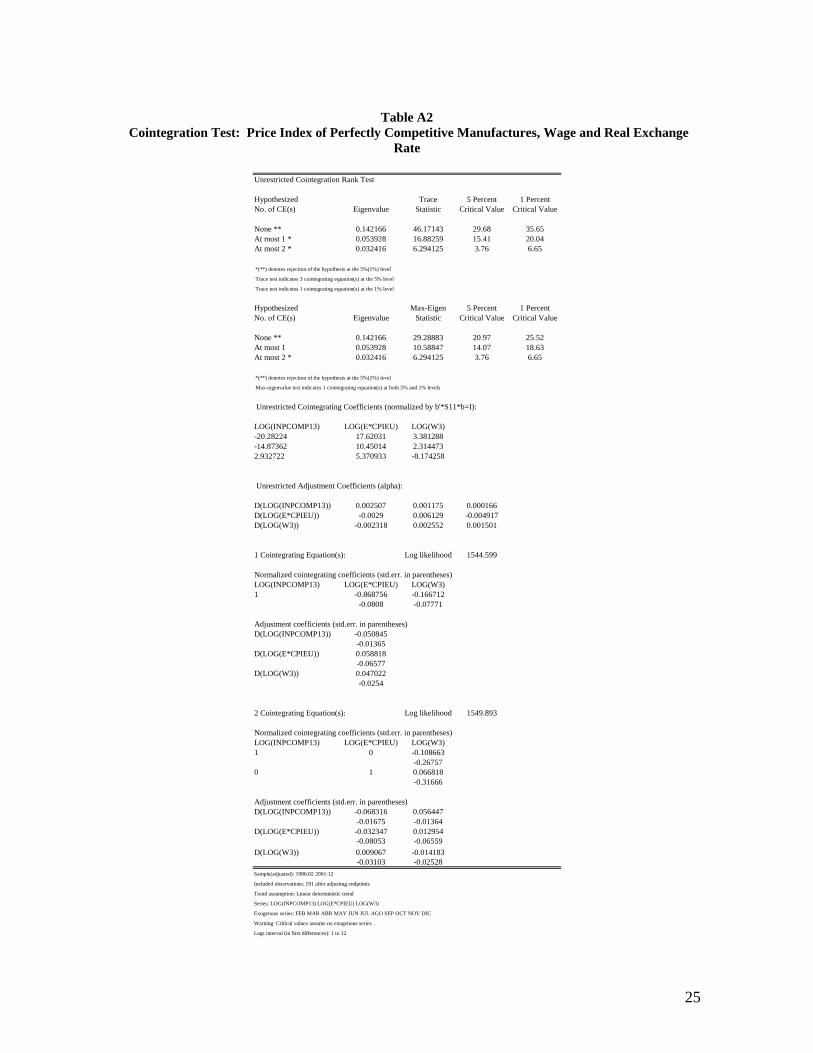
Table A2
Cointegration Test: Price Index of Perfectly Competitive Manufactures, Wage and Real Exchange Rate
Unrestricted Cointegration Rank Test
Hypothesized Trace 5 Percent 1 PercentNo. of CE(s) Eigenvalue Statistic Critical Value Critical Value
None ** 0.142166 46.17143 29.68 35.65At most 1 * 0.053928 16.88259 15.41 20.04At most 2 * 0.032416 6.294125 3.76 6.65
*(**) denotes rejection of the hypothesis at the 5%(1%) level
Trace test indicates 3 cointegrating equation(s) at the 5% level
Trace test indicates 1 cointegrating equation(s) at the 1% level
Hypothesized Max-Eigen 5 Percent 1 PercentNo. of CE(s) Eigenvalue Statistic Critical Value Critical Value
None ** 0.142166 29.28883 20.97 25.52At most 1 0.053928 10.58847 14.07 18.63At most 2 * 0.032416 6.294125 3.76 6.65
*(**) denotes rejection of the hypothesis at the 5%(1%) level
Max-eigenvalue test indicates 1 cointegrating equation(s) at both 5% and 1% levels
Unrestricted Cointegrating Coefficients (normalized by b'*S11*b=I):
LOG(INPCOMP13) LOG(E*CPIEU) LOG(W3)-20.28224 17.62031 3.381288-14.87362 10.45014 2.3144732.932722 5.370933 -8.174258
Unrestricted Adjustment Coefficients (alpha):
D(LOG(INPCOMP13)) 0.002507 0.001175 0.000166D(LOG(E*CPIEU)) -0.0029 0.006129 -0.004917D(LOG(W3)) -0.002318 0.002552 0.001501
1 Cointegrating Equation(s): Log likelihood 1544.599
Normalized cointegrating coefficients (std.err. in parentheses)LOG(INPCOMP13) LOG(E*CPIEU) LOG(W3)1 -0.868756 -0.166712
-0.0808 -0.07771
Adjustment coefficients (std.err. in parentheses)D(LOG(INPCOMP13)) -0.050845
-0.01365D(LOG(E*CPIEU)) 0.058818
-0.06577D(LOG(W3)) 0.047022
-0.0254
2 Cointegrating Equation(s): Log likelihood 1549.893
Normalized cointegrating coefficients (std.err. in parentheses)LOG(INPCOMP13) LOG(E*CPIEU) LOG(W3)1 0 -0.108663
-0.267570 1 0.066818
-0.31666
Adjustment coefficients (std.err. in parentheses)D(LOG(INPCOMP13)) -0.068316 0.056447
-0.01675 -0.01364D(LOG(E*CPIEU)) -0.032347 0.012954
-0.08053 -0.06559D(LOG(W3)) 0.009067 -0.014183
-0.03103 -0.02528Sample(adjusted): 1986:02 2001:12
Included observations: 191 after adjusting endpoints
Trend assumption: Linear deterministic trend
Series: LOG(INPCOMP13) LOG(E*CPIEU) LOG(W3)
Exogenous series: FEB MAR ABR MAY JUN JUL AGO SEP OCT NOV DIC
Warning: Critical values assume no exogenous series
Lags interval (in first differences): 1 to 12
26
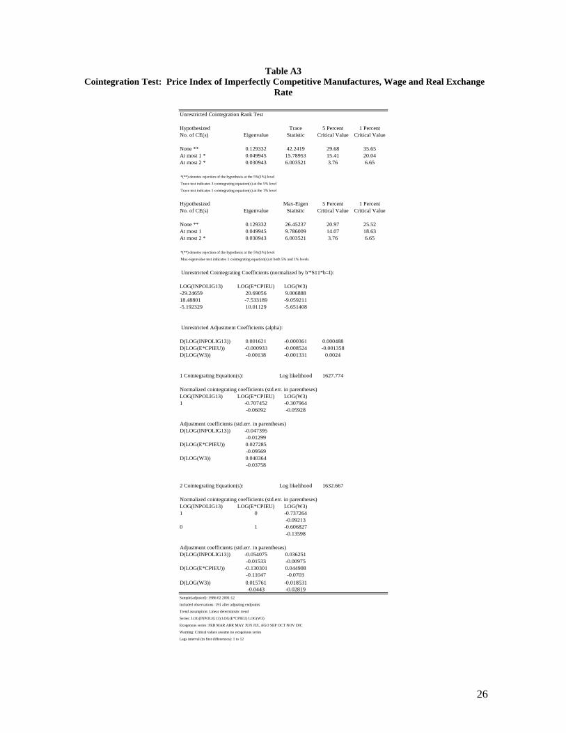
Table A3 Cointegration Test: Price Index of Imperfectly Competitive Manufactures, Wage and Real Exchange
Rate
Unrestricted Cointegration Rank Test
Hypothesized Trace 5 Percent 1 PercentNo. of CE(s) Eigenvalue Statistic Critical Value Critical Value
None ** 0.129332 42.2419 29.68 35.65At most 1 * 0.049945 15.78953 15.41 20.04At most 2 * 0.030943 6.003521 3.76 6.65
*(**) denotes rejection of the hypothesis at the 5%(1%) level
Trace test indicates 3 cointegrating equation(s) at the 5% level
Trace test indicates 1 cointegrating equation(s) at the 1% level
Hypothesized Max-Eigen 5 Percent 1 PercentNo. of CE(s) Eigenvalue Statistic Critical Value Critical Value
None ** 0.129332 26.45237 20.97 25.52At most 1 0.049945 9.786009 14.07 18.63At most 2 * 0.030943 6.003521 3.76 6.65
*(**) denotes rejection of the hypothesis at the 5%(1%) level
Max-eigenvalue test indicates 1 cointegrating equation(s) at both 5% and 1% levels
Unrestricted Cointegrating Coefficients (normalized by b'*S11*b=I):
LOG(INPOLIG13) LOG(E*CPIEU) LOG(W3)-29.24659 20.69056 9.00688818.48801 -7.533189 -9.059211-5.192329 10.01129 -5.651408
Unrestricted Adjustment Coefficients (alpha):
D(LOG(INPOLIG13)) 0.001621 -0.000361 0.000488D(LOG(E*CPIEU)) -0.000933 -0.008524 -0.001358D(LOG(W3)) -0.00138 -0.001331 0.0024
1 Cointegrating Equation(s): Log likelihood 1627.774
Normalized cointegrating coefficients (std.err. in parentheses)LOG(INPOLIG13) LOG(E*CPIEU) LOG(W3)1 -0.707452 -0.307964
-0.06092 -0.05928
Adjustment coefficients (std.err. in parentheses)D(LOG(INPOLIG13)) -0.047395
-0.01299D(LOG(E*CPIEU)) 0.027285
-0.09569D(LOG(W3)) 0.040364
-0.03758
2 Cointegrating Equation(s): Log likelihood 1632.667
Normalized cointegrating coefficients (std.err. in parentheses)LOG(INPOLIG13) LOG(E*CPIEU) LOG(W3)1 0 -0.737264
-0.092130 1 -0.606827
-0.13598
Adjustment coefficients (std.err. in parentheses)D(LOG(INPOLIG13)) -0.054075 0.036251
-0.01533 -0.00975D(LOG(E*CPIEU)) -0.130301 0.044908
-0.11047 -0.0703D(LOG(W3)) 0.015761 -0.018531
-0.0443 -0.02819Sample(adjusted): 1986:02 2001:12
Included observations: 191 after adjusting endpoints
Trend assumption: Linear deterministic trend
Series: LOG(INPOLIG13) LOG(E*CPIEU) LOG(W3)
Exogenous series: FEB MAR ABR MAY JUN JUL AGO SEP OCT NOV DIC
Warning: Critical values assume no exogenous series
Lags interval (in first differences): 1 to 12
27
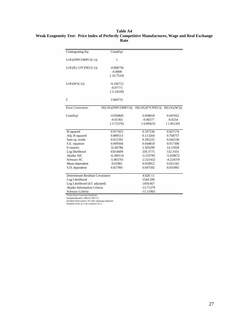
Table A4 Weak Exogeneity Test: Price Index of Perfectly Competitive Manufactures, Wage and Real Exchange
Rate
Cointegrating Eq: CointEq1
LOG(INPCOMP13(-1)) 1
LOG(E(-1)*CPIEU(-1)) -0.868756-0.0808
[-10.7519]
LOG(W3(-1)) -0.166712-0.07771
[-2.14528]
C 2.660731
Error Correction: D(LOG(INPCOMP13)) D(LOG(E*CPIEU)) D(LOG(W3))
CointEq1 -0.050845 0.058818 0.047022-0.01365 -0.06577 -0.0254
[-3.72376] [ 0.89425] [ 1.85120]
R-squared 0.917425 0.337236 0.827176 Adj. R-squared 0.889513 0.113204 0.768757 Sum sq. resids 0.012292 0.285225 0.042538 S.E. equation 0.009304 0.044818 0.017308 F-statistic 32.86786 1.505299 14.15928 Log likelihood 650.6609 350.3775 532.1031 Akaike AIC -6.300114 -3.155785 -5.058672 Schwarz SC -5.465761 -2.321432 -4.224319 Mean dependent 0.01965 0.018912 0.021242 S.D. dependent 0.027991 0.047592 0.035992
Determinant Residual Covariance 4.62E-11 Log Likelihood 1544.599 Log Likelihood (d.f. adjusted) 1459.667 Akaike Information Criteria -13.71379 Schwarz Criteria -11.15965 Vector Error Correction Estimates Sample(adjusted): 1986:02 2001:12 Included observations: 191 after adjusting endpoints Standard errors in ( ) & t-statistics in [ ]

28
Table A5 Weak Exogeneity Test: Price Index of Imperfectly Competitive Manufactures, Wage and Real
Exchange Rate
Cointegrating Eq: CointEq1
LOG(INPOLIG13(-1)) 1
LOG(E(-1)*CPIEU(-1)) -0.707452-0.06092
[-11.6119]
LOG(W3(-1)) -0.307964-0.05928
[-5.19506]
C 2.222568
Error Correction: D(LOG(INPOLIG13)) D(LOG(E*CPIEU)) D(LOG(W3))
CointEq1 -0.047395 0.027285 0.040364-0.01299 -0.09569 -0.03758
[-3.64960] [ 0.28514] [ 1.07396]
R-squared 0.955085 0.325345 0.818028 Adj. R-squared 0.939903 0.097293 0.756517 Sum sq. resids 0.005347 0.290342 0.044789 S.E. equation 0.006137 0.045218 0.01776 F-statistic 62.90754 1.426624 13.29879 Log likelihood 730.149 348.6792 527.1775 Akaike AIC -7.13245 -3.138002 -5.007094 Schwarz SC -6.298097 -2.303649 -4.172742 Mean dependent 0.020174 0.018912 0.021242 S.D. dependent 0.025032 0.047592 0.035992
Determinant Residual Covariance 1.93E-11 Log Likelihood 1627.774 Log Likelihood (d.f. adjusted) 1542.842 Akaike Information Criteria -14.58473 Schwarz Criteria -12.03059 Vector Error Correction Estimates Sample(adjusted): 1986:02 2001:12 Included observations: 191 after adjusting endpoints Standard errors in ( ) & t-statistics in [ ]
29
Table A6 Estimation Results of Price Error Correction Models of Manufactures with Import Penetration Rate
above and below 30 Percent Dependent Variable c2 c3 c4 c5 c6 c7 Adj. R2 F-stat. Prob(F-stat)
Coeff. 0.00356 0.02365 -0.02983 0.77127 0.05345 0.03592 0.92708 168.5264 0 Std. Error 0.00257 0.00666 0.00877 0.07244 0.01851 0.02024 t-Stat. 1.38722 3.55164 -3.40210 10.64752 2.88845 1.77434
PRICE INDEX OF MANUFACTURES WITH IMP. PEN >30%
Prob. 0.16690 0.00050 0.00080 0.00000 0.00430 0.07750
Coeff. 0.00615 0.03431 -0.04378 0.72725 0.03638 0.02745 0.92024 153.0212 0 Std. Error 0.00304 0.00807 0.01088 0.08572 0.02124 0.02062 t-Stat. 2.02004 4.25486 -4.02503 8.48359 1.71310 1.33096
PRICE INDEX OF MANUFACTURES WITH IMP. PEN >30% AND ψ* =1
Prob. 0.04470 0.00000 0.00010 0.00000 0.08820 0.18470
Coeff. 0.00882 0.02416 -0.03421 0.76490 0.09218 0.02191 0.89887 118.1188 0 Std. Error 0.00414 0.00659 0.00880 0.05564 0.03312 0.01288 t-Stat. 2.13197 3.66479 -3.88952 13.74777 2.78321 1.70102
PRICE INDEX OF MANUFACTURES WITH IMP. PEN >30% AND ψ* <1
Prob. 0.03420 0.00030 0.00010 0.00000 0.00590 0.09040
Coeff. 0.01252 0.04375 -0.05878 0.66556 0.11335 0.02708 0.88499 102.3863 0 Std. Error 0.00423 0.01050 0.01351 0.07849 0.03160 0.01548 t-Stat. 2.95958 4.16882 -4.35210 8.47978 3.58735 1.74968
PRICE INDEX OF MANUFACTURES WITH IMP. PEN <30%
Prob.
0.00340 0.00000 0.00000 0.00000 0.00040 0.08170
Coeff. 0.00964 0.02908 -0.04031 0.58733 0.08845 0.00682 0.78272 48.46494 0 Std. Error 0.00655 0.00607 0.00879 0.09284 0.02937 0.01789 t-Stat. 1.47061 4.79289 -4.58858 6.32661 3.01178 0.38129
PRICE INDEX OF MANUFACTURES WITH IMP. PEN <30% AND ψ* =1
Prob. 0.14290 0.00000 0.00000 0.00000 0.00290 0.70340
Coeff. 0.01011 0.04860 -0.06218 0.60535 0.14006 0.03490 0.84177 71.09921 0 Std. Error 0.00426 0.01241 0.01527 0.08437 0.03738 0.02077 t-Stat. 2.37306 3.91506 -4.07239 7.17473 3.74672 1.68072
PRICE INDEX OF MANUFACTURES WITH IMP. PEN <30% AND ψ* <1
Prob. 0.01860 0.00010 0.00010 0.00000 0.00020 0.09430 Method: Least Squares Sample(adjusted): 1985:02 2003:10 Included observations: 225 after adjusting endpoints Newey-West HAC Standard Errors & Covariance (lag truncation=4)
Table A7 Pass-Through Coefficients of Wage and Exchange Rate of Manufactures with Import Penetration Rate
above and below 30 Percent
Dependent Variable λw λe
PRICE INDEX OF MANUFACTURES WITH IMP. PEN >30% 0.1195 0.7928
PRICE INDEX OF MANUFACTURES WITH IMP. PEN >30% AND ψ* =1 0.1404 0.7838
PRICE INDEX OF MANUFACTURES WITH IMP. PEN >30% AND ψ* <1 0.2577 0.7062
PRICE INDEX OF MANUFACTURES WITH IMP. PEN <30% 0.2129 0.7443
PRICE INDEX OF MANUFACTURES WITH IMP. PEN <30% AND ψ* =1 0.2390 0.7214
PRICE INDEX OF MANUFACTURES WITH IMP. PEN <30% AND ψ* <1 0.1626 0.7815 Wald Coefficient tests. *** Significant at the 1% level, ** Significant at the 5% level, * Significant at the 10% level
30
Graph A1 Rolling Regression Estimates of the Labor Cost Coefficient Using Different Wage Measures
Perfectly Competitive Manufactures
-0.1
-0.05
0
0.05
0.1
0.15
0.2
1998
:03:
00
1998
:06:
00
1998
:09:
00
1998
:12:
00
1999
:03:
00
1999
:06:
00
1999
:09:
00
1999
:12:
00
2000
:03:
00
2000
:06:
00
2000
:09:
00
2000
:12:
00
2001
:03:
00
2001
:06:
00
2001
:09:
00
2001
:12:
00
IMSS w age quotation Wage index of Perfectly Competitive Manufactures
Imperfectly Competitive Manufactures
-0.0600
-0.0400
-0.0200
0.0000
0.0200
0.0400
0.0600
0.0800
0.1000
0.1200
1998
:03:
00
1998
:06:
00
1998
:09:
00
1998
:12:
00
1999
:03:
00
1999
:06:
00
1999
:09:
00
1999
:12:
00
2000
:03:
00
2000
:06:
00
2000
:09:
00
2000
:12:
00
2001
:03:
00
2001
:06:
00
2001
:09:
00
2001
:12:
00
IMSS Wage Quotation Wage Index of Imperfectly Competitive Manufactures

31
Graph A2 Stability Tests of the equation for the Price Index of Perfectly Competitive Manufactures
A.2.1 Recursive residuals
-.08
-.06
-.04
-.02
.00
.02
.04
.06
.08
88 90 92 94 96 98 00 02
Recursive Residuals ± 2 S.E.
A.2.2 CUSUM test
-60
-40
-20
0
20
40
60
88 90 92 94 96 98 00 02
CUSUM 5% Significance
A.2.3 CUSUM of Squares test
-0.2
0.0
0.2
0.4
0.6
0.8
1.0
1.2
88 90 92 94 96 98 00 02
CUSUM of Squares 5% Significance
A.2.4 One Step Forecast Test
.00
.05
.10
.15
-.08
-.04
.00
.04
.08
88 90 92 94 96 98 00 02
One-Step Probability Recursive Residuals
A.2.5 N-Step Forecast Test
.00
.05
.10
.15 -.08
-.04
.00
.04
.08
88 90 92 94 96 98 00 02
N-Step Probability Recursive Residuals

32
A.2.6 Recursive estimates of the error correction term coefficients c2, c3 and c4
-.2
-.1
.0
.1
.2
.3
.4
88 90 92 94 96 98 00 02
Recursive C(2) Estimates ± 2 S.E.
-.04
-.02
.00
.02
.04
.06
.08
.10
88 90 92 94 96 98 00 02
Recursive C(3) Estimates ± 2 S.E.
-.4
-.3
-.2
-.1
.0
.1
88 90 92 94 96 98 00 02
Recursive C(4) Estimates ± 2 S.E.

33
Graph A3 Stability Tests of the equation for the Price Index of Imperfectly Competitive Manufactures
A.3.1 Recursive residuals
-.04
-.03
-.02
-.01
.00
.01
.02
.03
88 90 92 94 96 98 00 02
Recursive Residuals ± 2 S.E.
A.3.4 One Step Forecast Test
.00
.05
.10
.15
-.04
-.02
.00
.02
.04
88 90 92 94 96 98 00 02
One-Step Probability Recursive Residuals
A.3.2 CUSUM Test
-60
-40
-20
0
20
40
60
88 90 92 94 96 98 00 02
CUSUM 5% Significance
A.3.5 N-Step Forecast Test
.00
.05
.10
.15 -.04
-.02
.00
.02
.04
88 90 92 94 96 98 00 02
N-Step Probability Recursive Residuals
A.3.3 CUSUM of Squares Test
-0.2
0.0
0.2
0.4
0.6
0.8
1.0
1.2
88 90 92 94 96 98 00 02
CUSUM of Squares 5% Significance

34
A.3.6 Recursive estimates of the error correction term coefficients c2, c3 and c4
-.2
-.1
.0
.1
.2
.3
.4
88 90 92 94 96 98 00 02
Recursive C(2) Estimates ± 2 S.E.
-.04
-.02
.00
.02
.04
.06
.08
.10
88 90 92 94 96 98 00 02
Recursive C(3) Estimates ± 2 S.E.
-.5
-.4
-.3
-.2
-.1
.0
.1
.2
88 90 92 94 96 98 00 02
Recursive C(4) Estimates ± 2 S.E.

35
Graph A4 Rolling Regression Estimates of the Price Equation Error Correction Term’s Coefficients
Dependent Variable: Price Index of Perfectly Competitive Manufactures
Dependent Variable: Price Index of Imperfectly Competitive Manufactures
-0.025
0
0.025
0.05
0.075
0.1
0.125
1993
:11:
00
1994
:05:
00
1994
:11:
00
1995
:05:
00
1995
:11:
00
1996
:05:
00
1996
:11:
00
1997
:05:
00
1997
:11:
00
1998
:05:
00
1998
:11:
00
1999
:05:
00
1999
:11:
00
2000
:05:
00
2000
:11:
00
2001
:05:
00
2001
:11:
00
2002
:05:
00
2002
:11:
00
2003
:05:
00
Rolling regression log(w) coefficient estimate
Estimate-2 std. dev.
Estimate+2 std. dev.
-0.025
0
0.025
0.05
0.075
0.1
0.125
1993
:11:
00
1994
:05:
00
1994
:11:
00
1995
:05:
00
1995
:11:
00
1996
:05:
00
1996
:11:
00
1997
:05:
00
1997
:11:
00
1998
:05:
00
1998
:11:
00
1999
:05:
00
1999
:11:
00
2000
:05:
00
2000
:11:
00
2001
:05:
00
2001
:11:
00
2002
:05:
00
2002
:11:
00
2003
:05:
00
Rollign regression log(w) coefficient estimate
Estimate-2 std. dev.
Estimate+2 std. dev.
-0.075
-0.05
-0.025
0
0.025
0.05
0.075
0.1
0.125
0.15
1993
:11:
00
1994
:05:
00
1994
:11:
00
1995
:05:
00
1995
:11:
00
1996
:05:
00
1996
:11:
00
1997
:05:
00
1997
:11:
00
1998
:05:
00
1998
:11:
00
1999
:05:
00
1999
:11:
00
2000
:05:
00
2000
:11:
00
2001
:05:
00
2001
:11:
00
2002
:05:
00
2002
:11:
00
2003
:05:
00
Rolling regression log(e) coefficient estimate
Estimate-2 std. dev.
Estimate + 2 std. dev.
-0.05
-0.025
0
0.025
0.05
0.075
0.1
0.125
0.15
1993
:11:
00
1994
:04:
00
1994
:09:
00
1995
:02:
00
1995
:07:
00
1995
:12:
00
1996
:05:
00
1996
:10:
00
1997
:03:
00
1997
:08:
00
1998
:01:
00
1998
:06:
00
1998
:11:
00
1999
:04:
00
1999
:09:
00
2000
:02:
00
2000
:07:
00
2000
:12:
00
2001
:05:
00
2001
:10:
00
2002
:03:
00
2002
:08:
00
2003
:01:
00
2003
:06:
00
Rolling regression log(e) coefficient estimate
Estimate-2 std. dev.
Estimate+2 std.dev.
-0.3-0.275-0.25
-0.225-0.2
-0.175-0.15
-0.125-0.1
-0.075-0.05
-0.0250
0.025
1993
:11:
00
1994
:05:
00
1994
:11:
00
1995
:05:
00
1995
:11:
00
1996
:05:
00
1996
:11:
00
1997
:05:
00
1997
:11:
00
1998
:05:
00
1998
:11:
00
1999
:05:
00
1999
:11:
00
2000
:05:
00
2000
:11:
00
2001
:05:
00
2001
:11:
00
2002
:05:
00
2002
:11:
00
2003
:05:
00
Rolling regression log(p) coefficient estimate
Estimate-2 std. dev.Estimate+2 std. dev.
-0.3-0.275-0.25
-0.225-0.2
-0.175-0.15
-0.125-0.1
-0.075-0.05
-0.0250
0.025
1993
:11:
00
1994
:05:
00
1994
:11:
00
1995
:05:
00
1995
:11:
00
1996
:05:
00
1996
:11:
00
1997
:05:
00
1997
:11:
00
1998
:05:
00
1998
:11:
00
1999
:05:
00
1999
:11:
00
2000
:05:
00
2000
:11:
00
2001
:05:
00
2001
:11:
00
2002
:05:
00
2002
:11:
00
2003
:05:
00
Rolling regression log(p) coefficient estimate
Estimate-2 std. dev.
Estimate+2 std. dev.
Recommended
![Micro foundations of coping with innovation ... - IMP Group · [1] Micro foundations of coping with innovation paradoxes in networked NPD processes: Two prospective longitudinal cases](https://img.pdfslide.net/doc/110x75/5e560c27b1f71168a829e984/micro-foundations-of-coping-with-innovation-imp-1-micro-foundations-of-coping.jpg)