1
Innovation spillovers and firm performance:
Micro evidence from Spain (2004-2009)
Esther Goyaa, Esther Vayá, Jordi Suriñach
AQR-IREA Research Group, University of Barcelona
Av. Diagonal 690, Tower IV, Faculty of Economics and Business, Barcelona, Spain
a Corresponding author: [email protected] (+34) 93 402 19 84
This article analyses the impact that R&D expenditures and intra- and inter-industry externalities have on
the performance of Spanish firms. Despite the extensive literature studying the relationship between
innovation and productivity, there are far fewer studies in this particular area examining the importance
of sectoral externalities, especially focused on Spain. One novelty of this study, conducted for the
industrial and service sectors, is that we also consider the technology level of the sector in which the firm
operates and firm size. The database used is the Technological Innovation Panel (PITEC). It comprises
9,985 firms over the period 2004-2009 and has been used infrequently for studies of this type. The Olley
and Pakes (1996) estimator is adopted in order to account for both simultaneity and selection biases
providing consistent estimates. The results suggest that, unlike previous studies, R&D expenditures do
not have a direct impact on firm performance. By contrast, spillovers do. In particular, intra-industry
externalities present a positive and significant effect in low-tech and large firms. Inter-industry
externalities, however, present an ambiguous effect and there appears to be no specific pattern of
behaviour associated with technology level or firm size.
Keywords: Firm performance, innovation, sectoral externalities, firm size
JEL classification: D24, O33
2
1. Introduction
It is widely acknowledged that if a firm can increase its productivity it is likely to gain in
competitiveness, an essential attribute in today’s globalized world. This is of particular relevance
in the case of Spain, because even though productivity has increased in recent years (Figure 1),
this growth is largely attributable to a drastic reduction in employment (see Table 1).
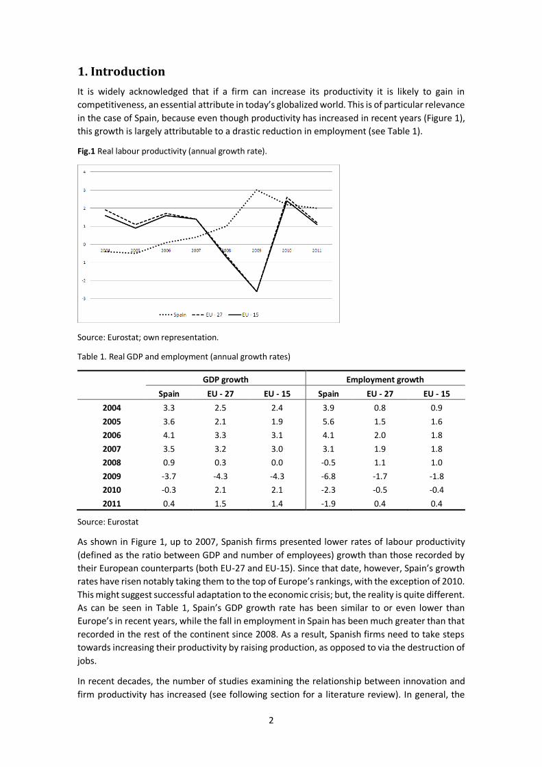
Fig.1 Real labour productivity (annual growth rate).
Source: Eurostat; own representation.
Table 1. Real GDP and employment (annual growth rates)
GDP growth Employment growth
Spain EU - 27 EU - 15 Spain EU - 27 EU - 15
2004 3.3 2.5 2.4 3.9 0.8 0.9
2005 3.6 2.1 1.9 5.6 1.5 1.6
2006 4.1 3.3 3.1 4.1 2.0 1.8
2007 3.5 3.2 3.0 3.1 1.9 1.8
2008 0.9 0.3 0.0 -0.5 1.1 1.0
2009 -3.7 -4.3 -4.3 -6.8 -1.7 -1.8
2010 -0.3 2.1 2.1 -2.3 -0.5 -0.4
2011 0.4 1.5 1.4 -1.9 0.4 0.4
Source: Eurostat
As shown in Figure 1, up to 2007, Spanish firms presented lower rates of labour productivity
(defined as the ratio between GDP and number of employees) growth than those recorded by
their European counterparts (both EU-27 and EU-15). Since that date, however, Spain’s growth
rates have risen notably taking them to the top of Europe’s rankings, with the exception of 2010.
This might suggest successful adaptation to the economic crisis; but, the reality is quite different.
As can be seen in Table 1, Spain’s GDP growth rate has been similar to or even lower than
Europe’s in recent years, while the fall in employment in Spain has been much greater than that
recorded in the rest of the continent since 2008. As a result, Spanish firms need to take steps
towards increasing their productivity by raising production, as opposed to via the destruction of
jobs.
In recent decades, the number of studies examining the relationship between innovation and
firm productivity has increased (see following section for a literature review). In general, the

3
findings stress the importance of R&D as a determinant of economic performance. Yet, as Figure
2 highlights, Spain’s business R&D to GDP ratio is much lower than that of the European Union
and, moreover, since 2008 it has gone into decline.
Fig.2 Business sector expenditure on R&D (% of GDP ratio).
Source: Eurostat; own representation.
Therefore, examining Spain’s R&D-productivity relationship in greater depth is essential if we
are to further our understanding of it and if we hope to design policies that can raise
productivity, especially in the current economic climate. For this reason, the primary goal of this
paper is to analyse the relationship between R&D and firm performance in Spain over the last
few years. In the light of previous studies that report differences in the productivity gains
attributable to innovation in accordance with a firm’s level of technology and size, and given
that few studies of the Spanish case take these two factors into account, here we assess whether
differences can be found between high- and low-tech firms, as well as between small and large
firms1.
Additionally, it should be borne in mind that the knowledge derived from a firm’s investment in
innovation is likely to spill over, given its inability to reap all the benefits from its investment.
Therefore, when examining the impact of innovation on productivity, the diffusion of the
innovation and any externalities generated also need to be taken into account. Several papers
have analysed the importance of spillovers; however, there has been little discussion about this
aspect from a sectoral perspective, particularly in Spain. Thus, the second goal of this paper is
to study the extent to which a firm’s performance is influenced by the innovation carried out by
other firms in the same sector (intra-industry externality) or by the innovation activities of firms
in other sectors (inter-industry externality).
1 It should be mentioned that Goya et al. (2012) carry out a similar analysis; however it is a much basic
work using cross-section data for 2010. In the present paper we use panel data and we are able to capture
changes over time as well as tackle several problems that appear when a productivity analysis is
undertaken. Unobserved heterogeneity or simultaneity issues need to be taking into account since they
might be affecting the relationship between innovation and productivity. The estimation method used
here (Olley and Pakes, 1996) account for these problems providing consistent results.
0,00
0,20
0,40
0,60
0,80
1,00
1,20
1,40
2005 2006 2007 2008 2009 2010
EU-27 EU-15 Spain

4
The study is conducted using the Technological Innovation Panel (PITEC) database, an
unbalanced panel of 9,985 Spanish firms from both the industrial and service sectors for the
period 2004 to 2009. It should be stressed that the study breaks new ground, since not only
examines the situation for the whole country but also for the industrial and service sectors. By
doing so, it aims to overcome a severe limitation given that most studies to date have focused
solely on the manufacturing sector or have covered only a specific region (as we shall see below).
In addition, PITEC contains a high level of sectoral information which enables us to focus our
attention on inter-industry externalities as well. Finally, the Olley and Pakes (1996) estimator is
adopted in order to account for unobserved heterogeneity, simultaneity issues and selection
bias. These are common problems that arise when a productivity analysis is carried out.
However, by using this method, consistent and reliable coefficients can be obtained.
To sum up, the aim of this paper is twofold. First, it seeks to analyse the extent to which the
technology level2 and size of Spanish firms affect the impact that R&D expenditures might have
on firm performance over the period 2004-2009. In other words, it investigates if there are
differences regarding the contribution of R&D in firm performance between low-tech and high-
tech firms as well as between small and large firms. Second, it assesses how these factors
influence potential knowledge flows from other firms’ innovations, both intra- and inter-
industry externalities. Thus, this article aims to answer the following questions: (i) Does the
impact of R&D on firm performance differ according to a firm’s technology level and/or firm
size? (ii) Are Spanish firms able to benefit from externalities? (iii) And if so, do these benefits
vary according to a firm’s technology level and/or firm size?
This paper has been organized as follows. Section 2 examines the previous literature, Section 3
presents the theoretical model, Section 4 describes the database and empirical model, Section
5 presents the results, and finally the conclusions are drawn in Section 6.
2. Previous Literature
A considerable body of literature has been published since Griliches (1979, 1986) first examined
the link between innovation and productivity. The well-known Cobb-Douglas production
function is normally used to conduct the empirical analysis, with the traditional inputs of physical
capital and labour being extended to include innovation expenditures. In general, the evidence
reveals a positive and significant relationship between innovation and productivity at the firm
level (see Mairesse and Sassenou 1991 for a detailed study, and also – to name but a few – Hall
and Mairesse 1995 for France; Harhoff 1998 for Germany; Lotti and Santarelli 2001 for a
comparative study of Germany and Italy; Parisi et al. 2006 for Italy and Ballot et al. 2006 for
France and Sweden). However, the results obtained seem to depend on the geographical area
being analysed as well as on the nature of the database and methodology used.
2 By technology level we mean the level of technology of the sector in which the firm operates. As it will
be seen in section 4.1 firms can be classified as high-tech manufacturing industries (HTMI), low-tech
manufacturing industries (LTMI), knowledge-intensive services (KIS) and non-knowledge intensive
services (NKIS). This is an interesting factor to include in the analysis as technological opportunities and
appropriability conditions are different between sectors which can lead to differences in the influence of
R&D. According to previous studies (see next section), investments in R&D carried out by firms operating
in “more advanced” sectors (HTMI and KIS) are more fruitful in increasing firm´s productivity than
investments undertake by firms operating in “less advanced” sectors (LTMI and NKIS).

5
It is worth mentioning that most of these articles undertake cross-country analyses, and pay
scant attention to the impact that a firm’s sector or size might have. As stressed in the previous
section, our primary goal is to determine whether there are any differences in the impact of
innovation on firm performance according to these factors. Empirical evidence to date suggests
that the impact of R&D expenditures on a firm’s productivity is more marked in high-tech sectors
than it is in their low-tech counterparts (see Verspagen 1995 for nine OECD countries; Tsai and
Wang 2004 for Taiwan; Ortega-Argilés et al. 2010 and 2011 for European firms). As regards firm
size, we are interested in determining whether size influences the returns firms obtain from
innovation, taking into consideration that the larger the firm, the more innovation it is likely to
conduct (see Huergo and Jaumandreu 2004). However, very little research has been published
in the literature on this question. According to Castany et al. (2009), the size of Spanish firms
does have an influence on the returns obtained from investment in both innovation and human
capital, with the largest firms being the ones that benefit most from these investments.
In addition, this article seeks to determine if the stock of knowledge available at the firm level is
dependent on both the firm’s own innovation or on externalities. As discussed above, the
benefits derived from innovation in a firm (or sector) are likely to spill over because of the firm’s
inability to channel all of the benefits obtained from its investment effort. Thus, a firm’s
performance can be explained by its own knowledge as well as by the knowledge generated
somewhere else which is in the public domain. For this reason, externalities need to be taken
into consideration.
From an empirical perspective, most articles employ a production function where spillovers are
included as an additional input (following Griliches 1979). Although there has been a
considerable number of studies that have analysed the impact of R&D spillovers on productivity,
a general consensus has yet to be reached on just what that effect might be. Despite the positive
impact reported by some authors (Griliches 1992; Nadiri 1993; Cincera 2005; Wieser 2005; Aiello
and Cardamone 2005 and 2008; Cardamore 2012 and Bloch 2013), others draw different
conclusions (see, for example, Klette 1994 for Norway; Los and Verspagen 2000 for U.S. firms;
Harhoff 2000 for Germany; Wakelin 2001 for the United Kingdom; Rogers 2010 for United
Kingdom; Medda and Piga 2014 for Italy). Overall, the evidence is unclear, with spillovers having
an apparently heterogeneous effect (being positive, negative or not significant). Yet, it should
be borne in mind that the results are conditioned by the sector or country under analysis and
that they are highly dependent on the way in which externalities are quantified (using
technological similarity, geographical distance or commercial relations).
As far as Spain is concerned, the relationship between innovation and productivity has been
examined by a number of authors, who conclude that innovation has a positive impact on
productivity. However, a general limitation of most of these studies is that their analyses are
restricted to manufacturing firms based on the Encuesta sobre Estrategias Empresariales
dataset (ESEE)3. Among the most recent papers employing this database we find Vivero (2002),
Huergo and Moreno (2004), Huergo and Jaumandreu (2004), Maté-García and Rodríguez-
Fernández (2002, 2008), Rodríguez-Fernández and Maté-García (2006), Rochina-Barrachina et
al. (2010) and Casiman et al. (2010), to name but a few. By contrast, only a few papers have
carried out a joint analysis of both manufacturing and service sectors, most notably Segarra-
3 The ESEE is a firm-level survey of Spanish manufacturing which collects annual information since 1990.

6
Blasco (2010) and Segarra-Blasco and Teruel (2011) who analyse the case of Catalonia using data
from the fourth Community Innovation Survey (CIS4).
In the case of external knowledge, far too little attention has been paid to the effect of spillovers
on the productivity of Spanish firms. Some articles, including Ornaghi (2006), argue that
externalities are positive and significant in explaining productivity. In this study the impact of
spillovers on productivity growth is examined in 3,151 manufacturing firms from 1990 to 1999.
Spillovers are measured by taking into account firm size and the results indicate a positive impact
of technological externalities on growth in productivity. However, the results in other studies
differ according to the economic sector in which the firm operates and its level of technology.
For instance, Beneito (2001) analyses the impact of intra-industry externalities on productivity
for 501 Spanish manufacturing firms distinguishing them according to technology level during
the period 1990-96. The author concludes that only firms using advanced technologies are able
to benefit from the knowledge in their technological neighbourhood. In particular, the spillover
effect depends on the intensity of R&D, with firms in the intermediate quartile being the ones
that experience the largest productivity gains.
All in all, the question that still needs to be addressed is whether differences are to be found in
the returns that Spanish firms obtain from their innovation investments in relation to their
technology level or firm size. In addition, given the paucity of studies assessing the impact of
spillovers in Spain, this paper will examine if firms in the sample are able to benefit from the
innovation carried out by others.
3. Economic model
The model adopted to estimate the relationship between innovation and firm performance is
the extended Cobb-Douglas production function, which apart from including conventional
production factors (physical capital and labour) also incorporates human capital and
innovation4. In line with previous studies5, it is believed that the more qualified workers the firm
has, the more effectively they are likely to perform their tasks and the more productive the firm
is likely to be. Additionally, innovation, the variable of interest in this study, has been included
as a production input. Investment in innovation can reduce costs of production or raise firm
sales, thus increasing production.
𝑌𝑖𝑠𝑡 = 𝐴𝑖𝑠𝑡 ∙ 𝐾𝑖𝑠𝑡𝛽1 ∙ 𝐿𝑖𝑠𝑡
𝛽2 ∙ 𝐻𝑖𝑠𝑡𝛽3 ∙ 𝐼𝑖𝑠𝑡
𝛽4 [1]
where 𝑌𝑖𝑠𝑡 is the output of firm i belonging to sector s at year t, 𝐴𝑖𝑠𝑡 is the firm's technology
level, 𝐾𝑖𝑠𝑡 is physical capital, 𝐿𝑖𝑠𝑡 is labour, 𝐻𝑖𝑠𝑡 is human capital, 𝐼𝑖𝑠𝑡 is innovation and
𝛽1, 𝛽2, 𝛽3, 𝛽4 are the returns on each variable respectively.
Following Goya et al. (2012), it is assumed that firm's level of technology is dependent on the
innovation made by all the other firms:
4 It should be pointed out that only a few microeconomic studies, especially for the case of Spain, have
incorporated human capital and innovation as factors in the production function.
5 See for instance, Black and Lynch (1996) and Haltiwanger et al. (1999) for the United States, Turcotte
and Rennison (2004) for Canada, Arvanitis and Loukis (2009) for Greece and Switzerland, Yang et al. (2010)
for China and Lee (2011) for Malaysia.

7
𝐴𝑖𝑠𝑡 = 𝐴 ∙ (𝑆𝑖𝑠𝑡𝑖𝑛𝑡𝑟𝑎 )𝜙1 ∙ (𝑆𝑖𝑠𝑡
𝑖𝑛𝑡𝑒𝑟)𝜙2 [2]
where A is a constant denoting a common technology level for all the firms; 𝑆𝑖𝑠𝑡𝑖𝑛𝑡𝑟𝑎 is the intra-
industry externality of firm i in sector s capturing the innovative effort made by all the other
firms in the same sector; and 𝑆𝑖𝑠𝑡𝑖𝑛𝑡𝑒𝑟 is the inter-industry externality understood as the
innovation made by the firms in the rest of the sectors.
Thus by combining Equations [1] and [2] it can be seen that a firm's output is explained in terms
of its own investments (in physical capital, human capital and innovation) and of the knowledge
generated outside the firm:
𝑌𝑖𝑠𝑡 = 𝐴 ∙ 𝐾𝑖𝑠𝑡𝛽1 ∙ 𝐿𝑖𝑠𝑡
𝛽2 ∙ 𝐻𝑖𝑠𝑡𝛽3 ∙ 𝐼𝑖𝑠𝑡
𝛽4 ∙ (𝑆𝑖𝑠𝑡𝑖𝑛𝑡𝑟𝑎 )𝜙1 ∙ (𝑆𝑖𝑠𝑡
𝑖𝑛𝑡𝑒𝑟)𝜙2 [3]
Therefore, under the assumption that 𝜙1 ≠ 0 and 𝜙2 ≠ 0, even though a firm does not invest
in innovation, it can still benefit from the innovation carried out by all the other firms and,
thereby, increase its performance.
4. Data and empirical model
4.1. Data: Technology Innovation Panel (PITEC)
In the empirical analysis we use PITEC, which provides information on the innovation activities
of Spanish firms for the period 2003-20096. The National Institute of Statistics (INE), in
consultation with a group of experts and under the sponsorship of the Spanish Foundation for
Science and Technology (FECYT) and the Foundation for Technological Innovation (COTEC), is
responsible for building up this database. PITEC is built upon the Spanish Innovation Survey
carried out by the INE, which in turn is based on the Community Innovation Survey (CIS) which
follows guidelines laid down by the OECD's Oslo Manual and, through the use of a standardized
questionnaire, enables comparisons to be made between countries.
PITEC is a data panel based on a representative selection of firms, which makes it possible to
carry out repeated observations of the economic units included over time and thereby develop
much more precise estimations of the evolution of R+D+I activities in the business sector
(innovation expenditures, composition of the samples, etc.), determine the impact of innovation
(different effects on productivity) and identify the various strategies in the decisions adopted by
firms when introducing innovations into their business (for instance the different compositions
of internal and external R&D expenditures as a part of total expenditures). The panel is made up
of four non-excludable samples: (i) firms with 200 or more employees, (ii) firms with internal
R&D expenditures, (iii) firms with fewer than 200 employees with external R&D expenditures
but which carry out no internal R&D, and (iv) firms with fewer than 200 employees with no
innovation expenditures.
6 Last year available when this paper was written.
8
Although PITEC has provided statistical information since 2003, in this paper we only draw on
data for the period 2004-20097. After a filtering process8, only firms with ten or more employees9
operating in the industrial and service sectors were selected (primary sector and construction
were thus excluded). Note that the influence of extreme outliers in the sample was treated
accordingly (see appendix A). Our eventual sample consisted of an unbalanced panel of 9,985
firms (51,604 observations).
PITEC provides information on individual firm characteristics (sales, exports, employment, the
market in which a firm operates, industry sector, etc.) along with detailed information on
innovation activities, such as different types of innovation expenditures, cooperation between
firms, barriers to innovation and number of patents, etc.
There is a double advantage of using this database. Firstly it provides information on both the
industrial and service sectors, making possible to overcome the limitation that most studies in
Spain focus solely on the manufacturing sector, generally using the ESEE. Secondly, it contains a
high level of sectoral information covering 51 sectors (see appendix B). This level of detail
enables a rich study to be undertaken examining differences in behaviour between sectors with
different technology levels and, in turn, making a more interesting study of inter-industry
externalities possible.
In line with the aim of this paper and for the purposes of analysing whether the impact of
innovation and externalities on firms performance vary depending on the sector's technology
and firm size, the total sample of 9,985 firms has been divided up according to the technology
level of the sector in which the firm operates and also according to firm size. In the first case, we
have used the Eurostat classification and grouped the firms by sector into the following
categories: (a) low and medium-low tech manufacturing firms (LTMI), (b) medium-high and high-
tech manufacturing firms (HTMI), (c) non-knowledge-intensive services (NKIS) and (d)
knowledge-intensive services (KIS). In the second case, we have distinguished between: (a) small
firms (from 10 to 49 employees), (b) medium-sized firms (from 50 to 199 employees) and (c)
large firms (200 or more employees). To see the distribution of firms according to sub-samples
see appendix C.
4.2. Empirical model and estimation issues
According to the expression [3], and using the information supplied by the PITEC database10,
the following econometric model can be specified:
7 We do not use data for 2003 because of its severe limitations. PITEC began with just two samples in 2003
(a sample of firms with 200 or more employees and a sample of firms with internal R&D expenditures). In
2004, it overcame this limitation by including a sample of firms with fewer than 200 employees with
external R&D expenditures but which carried out no internal R&D and a sample of firms with fewer than
200 employees with no innovation expenditures.
8 This filtering process meant eliminating those observations that included any kind of ‘incident’ (i.e.,
confidentiality problems, takeovers, mergers, etc.) and those containing obvious anomalies (such as null
sales).
9 The population area is as defined by the Spanish Innovation Survey on which PITEC is based.
10 Unfortunately, PITEC does not contain information about intermediate consumptions, prices or other
information necessary to compute total factor productivity (or multi-factor productivity). Thereby, this

9
𝑦𝑖𝑠𝑡 = 𝛽0 + 𝛽1𝑘𝑖𝑠𝑡 + 𝛽2𝑙𝑖𝑠𝑡 + 𝛽3ℎ𝑖𝑠𝑡 + 𝛽4𝑖𝑖𝑠𝑡 + 𝜙1𝑆𝑖𝑠𝑡−2𝑖𝑛𝑡𝑟𝑎 + 𝜙2𝑆𝑖𝑠𝑡−2
𝑖𝑛𝑡𝑒𝑟 + 𝑐𝑜𝑛𝑡𝑟𝑜𝑙𝑠 + 𝑢𝑖𝑠𝑡 [4]
𝑢𝑖𝑠𝑡 = ω𝑖𝑠𝑡 + 휀𝑖𝑠𝑡 [5]
where 𝑦𝑖𝑠𝑡 approximates the sales, 𝑘𝑖𝑠𝑡 is the physical capital stock, 𝑙𝑖𝑠𝑡 is the number of
employees, ℎ𝑖𝑠𝑡 is the percentage of employees with higher education, and 𝑖𝑖𝑠𝑡 is defined as
R&D stock11. 𝑆𝑖𝑠𝑡𝑖𝑛𝑡𝑟𝑎 and 𝑆𝑖𝑠𝑡
𝑖𝑛𝑡𝑒𝑟 are the externalities defined below. The regression controls are
represented by technology level and firm size dummies and also a trend to capture time
changes12. On the other hand, 𝜔𝑖𝑠𝑡 is the productivity shock and 휀𝑖𝑠𝑡 is the error term (which can
contain unpredictable productivity shocks). Lower case letters indicates log-transformed
variables (with the exception of human capital which is a percentage). All monetary variables
are expressed at constant values at 2009 base prices (nominal values have been deflated using
the GDP deflator).
As is widely accepted in the literature13, a firm’s output is assumed to be affected by
accumulated stocks of physical capital and R&D expenditures, rather than by current flows. We
use the well-known perpetual inventory method:
𝐾𝑡 = 𝐾𝑡−1 ∙ (1 − 𝛿ℎ𝑘) + 𝐶𝑡
𝐾0 =𝐶0
𝑔𝑠𝑘+𝛿ℎ
𝑘
[6]
and
𝐼𝑡 = 𝐼𝑡−1 ∙ (1 − 𝛿ℎ𝑖 ) + 𝑅𝐷𝑡
𝐼0 =𝑅𝐷0
𝑔𝑠𝑖+𝛿ℎ
𝑖
[7]
with t = 2004, …, 2009 h = 1, 2, 3, 4 s = 1, ..., 51.
where 𝐶𝑡 is the real investment in material goods and 𝑅𝐷𝑡 are the real R&D expenditures. We
applied different depreciation rates according to the technology level (h). Following Ortega-
Argilés (2011), the more advanced the sector, the faster is the technological progress
accelerating the obsolescence of its current physical capital and knowledge. Thus, we applied
sectoral depreciation rates of 6% and 7% for physical capital (𝛿ℎ𝑘) and 15% and 18% for
innovation (𝛿ℎ𝑖 ) to low-tech and high-tech sectors respectively14. In the case of growth rates, if
we used the initial periods for their computation, we would lose a considerable amount of
kind of analysis is not possible here. The only measure available regarding output is firm sales (this is
something common when Innovation Surveys are used, for instance Community Innovation Survey).
11 We are aware that the concept of innovation is very wide including not only R&D expenditures, but
also, the acquisition of machinery, equipment and hardware/software, training staff directly involved in
developing the innovation, introduction innovation in the market, design, etc. However, in line with
previous studies, we approximate innovation with R&D expenditures (both internal and external).
12 Although industry dummies would capture technological opportunities as well as specificities of the
sector, we cannot include them since it would give rise to perfect multicollinearity with the inter-industry
externalities.
13 See Hall and Mairesse (1995), Bönte (2003) and Ortega-Argilés et al. (2011) to name just a few.
14 The results are almost identical if a fix depreciation rate is used (6% for physical capital and 15% for
innovation).

10
information given that our panel has a short time dimension (2004-2009). Thus, we opted to
calculate 𝑔𝑠𝑘 and 𝑔𝑠
𝑖 as the average rate of change in real investment in material goods and real
R&D expenditures in each sector(s) over the period 1995-200315. We used the OECD’s ANBERD
database to calculate physical capital growth rates (𝑔𝑠𝑘) and the OECD’s STAN database for
innovation growth rates(𝑔𝑠𝑖 ).
As regards externalities, due to the many different ways in which spillovers can occur (learning
what other firms do either via the movements of workers themselves or through reading articles
in journals, attending conferences, disclosure of patents, reverse-engineering, etc.), measuring
them is a far from easy task. We follow the definition adopted by Goya, et al. (2012) where the
authors use R&D expenditures to proxy external knowledge.
Thus, intra-industry externality is defined as:
𝑆𝑖𝑠𝑡𝑖𝑛𝑡𝑟𝑎 = ∑ 𝐼𝑗𝑠𝑡𝑗≠𝑖 [8]
where 𝐼𝑗𝑠𝑡 is total R&D stock carried out in sector s at time t (except the firm’s own R&D
investment). This definition is open to criticism since it attaches the same weight to all the firms
in the same sector. Thus, it assumes that the propensity to benefit from the R&D expenditures
in the sector is the same for all firms. However, by employing this definition, the technological
effort of the sector in which the firm is located is captured and so it serves as an indicator of the
magnitude of the technological effort currently available in the sector.
On the other hand, it can be supposed that firms which maintain commercial relationships
benefit from the knowledge embodied in the products in which they trade. Thus, the more they
buy and sell, the more they benefit from the knowledge originated in the other sector.
Therefore, inter-industry externality is defined in the following way:
𝑆𝑖𝑠𝑡𝑖𝑛𝑡𝑒𝑟 = ∑ 𝑤𝑠𝑚 ∙ 𝐼𝑗𝑚𝑡𝑚≠𝑠 [9]
where 𝐼𝑗𝑚𝑡 is R&D stock undertaken in all the other sectors and 𝑤𝑠𝑚 is defined as the quotient
between the intermediate purchase by sector s of goods and services supplied by sector m and
the total sum of intermediate purchase of sector s. Thus, the influence that the R&D
expenditures of firms in sector m have on the productivity of firm i in sector s is based on the
relative importance that sector m has as supplier to sector s. To construct the weights we use
the symmetric input-output table for Spain for 2005 (the latest year available). An exercise of
correspondence has had to be carried out between the branches of business activity according
to which PITEC data are classified and the branches of business activity in the input-output table.
As it has been seen in the literature review, both positive and negative coefficients are possible.
On the one hand, an external pool of knowledge is expected to have a positive impact on the
production of other firms, since they can benefit from new knowledge and ideas. However, on
the other hand, if rival firms increase their R&D investment a competitive effect might appear.
This is what some authors have called “market-stealing effect” (De Bondt, 1996; Bitzer and
15 Note, however, that the choice of g does not modify the results greatly. As Hall and Mairesse (1995)
report in footnote 9: “In any case, the precise choice of growth rate affects only the initial stock, and
declines in importance as time passes…”.
11
Geishecker, 2006; Bloom et al., 2013). Therefore, both possibilities need to be taken into
consideration.
As can be seen in expression [4], both externalities have been lagged two periods, since the
assumption of a contemporary relationship between them and firm performance seems
inappropriate, given that there is no immediate impact. On the contrary, it is likely that the
diffusion of external knowledge takes some time before it can affect the firm.
As far as the estimation method is concerned, it is well-known in the literature that estimates
from a production function may suffer from simultaneity as well as selection bias. As such, OLS
estimates are biased and inconsistent.
The former problem, simultaneity (first noted by Marschak and Andrews, 1944), arises because
productivity shocks (𝜔𝑖𝑠𝑡) are known to the firm but not to the econometrician. Thus, when the
firm has to determine the usage of inputs its decision is influenced by its beliefs about
productivity. Therefore, input choices will be correlated with productivity shocks. So if a firm
faces a positive (negative) productivity shock, its use of inputs is going to increase (decrease)
accordingly. Not taking this issue into consideration leads to biased and inconsistent estimates
since the error term is correlated with the explanatory variables (breaking one of the basic
hypotheses of OLS). The second problem, selection bias, manifests itself because of the exit of
inefficient firms (not randomly). A firm with higher capital is expected to obtain higher profits in
the future and so is more likely to stay in the market despite a negative productivity shock (given
that in the future it is thought it will produce more) than a firm with lower capital16.
In order to deal with these problems and to ensure the reliability of the coefficients we use the
estimator proposed by Olley and Pakes in 1996 (hereafter OP). Other methods are employed in
the literature, but they only address simultaneity bias17. In contrast, the OP estimator addresses
both simultaneity as well as selection bias18. For this reason, this estimation method has been
used by several authors who seek to analyse, for instance, the impact of trade and tariffs on firm
productivity (see for example, Pavcnick, 2002; Schor, 2004; Amiti and Koungs, 2007; De Loecker,
2007; Loung, 2011; Van Beveren, 2012 and Arvas and Uyar, 2014). While it is true that it is not
one of the most common approaches in the innovation literature, some papers have recently
applied this estimator to obtain unbiased and consistent estimates of the production function
(see Marrocu, et al.; 2011 and Añón-Higón and Manjón-Antonlín, 2012).
16 Even though the evidence suggests that simultaneity bias is more important than selection bias, the estimator used here controls for both.
17 As shown in the literature, simultaneity problems can be addressed by using instrumental variables or fixed effect estimators. However, given that the panel is short and instrumental variables use lagged values as instruments, their suitability is reduced (facing a problem of weak instruments). The fixed effects estimator, on the other hand, relies on the assumption that productivity shocks are constant over time, which is an excessively strong premise from our point of view, especially bearing in mind the economic situation in the period under analysis.
18 Another option might be the Levinsohn and Petrin (2003) estimator, but intermediate inputs are needed in this case (and this information is not provided by PITEC). Thus, we strongly believe that the best option available is the OP estimator.

12
4.2.1. Olley & Pakes (1996) estimator
Intuitively, the idea behind the OP method is to make “observable” the “unobservable”; in other
words, to use an equation to proxy for the unobserved productivity shock. By doing so, the
econometrician can control for the correlation between the error term and the inputs and
obtain consistent results. Below, the main features of the OP approach are described (using the
same notation as that employed by Olley and Pakes, 1996)19. After that, the changes introduced
in order to adapt the method to our case are explained.
First of all, Olley and Pakes base their analysis on the traditional Cobb-Douglass production
function:
𝑦𝑖𝑡 = 𝛽0 + 𝛽𝑎𝑎𝑖𝑡 + 𝛽𝑘𝑘𝑖𝑡 + 𝛽𝑙𝑙𝑖𝑡 + 𝑒𝑖𝑡 [10]
where the log of output (𝑦𝑖𝑡) is explained by the age of the firm (𝑎𝑖𝑡), the log of capital (𝑘𝑖𝑡), the
log of labour (𝑙𝑖𝑡) and an error term (𝑒𝑖𝑡) that is decomposed in two components: a productivity
shock (𝜔𝑖𝑡) and a measurement error term or unexpected productivity shock (𝜂𝑖𝑡). The former
is observed by the firm but not by the econometrician and affects the firm’s decision, while the
latter is unobserved by both and does not affect the firm’s decision.
As for the inputs in the production function, the authors differentiate between variable factors
(such as, 𝑙𝑖𝑡), which can be easily adjusted given a productivity shock, and fixed factors (also
known as “state variable”) which depend on information from the previous period and are costly
to adjust with productivity shocks (𝑘𝑖𝑡 and 𝑎𝑖𝑡).
As explained by the authors, at the beginning of every period an incumbent firm has to decide
whether to exit or to continue in the market. The firm remains in the market if the current state
variables indicate that the returns of staying in the business are higher than the sell-off value.
This is known as the “exit rule” and is specified as follows:
𝜒𝑡 = {1 𝑖𝑓 𝜔 ≥ 𝜔(𝑎𝑡 , 𝑘𝑡)
0 𝑜𝑡ℎ𝑒𝑟𝑤𝑖𝑠𝑒 [11]
where 𝜒𝑡 is an indicator function that takes a value of 1 if the firm remains in the market and 0
if the firm exits and 𝜔 is a productivity threshold that depends on the firm’s capital and age.
If the firm continues in the market, it chooses a level of inputs (𝑙𝑖𝑡) and a level of investment
according to 𝜔𝑖𝑡 , 𝑘𝑖𝑡 and 𝑎𝑖𝑡. This is known as the “investment decision rule”:
𝑖𝑖𝑡 = 𝑖( 𝜔𝑖𝑡 , 𝑘𝑖𝑡 , 𝑎𝑖𝑡) [12]
Provided that 𝑖 > 0 and investment is increasing in productivity, the investment function can be
inverted as follows: 𝜔 = ℎ( 𝑖𝑖𝑡 , 𝑘𝑖𝑡 , 𝑎𝑖𝑡) where ℎ(∙) = 𝑖−1(∙). As the authors put it “[this
expression] allows us to express the unobservable productivity variable, 𝜔𝑡 , as a function of
observables, and hence to control for 𝜔𝑡 in the estimation” (Olley and Pakes, 1996 page 1275).
The production function can then be rewritten as:
𝑦𝑖𝑡 = 𝛽𝑙𝑙𝑖𝑡 + 𝜙( 𝑖𝑖𝑡 , 𝑘𝑖𝑡 , 𝑎𝑖𝑡) + 𝜂𝑖𝑡 [13]
19 For a detailed explanation of the equations and estimation strategy see Olley and Pakes (1996).

13
where 𝜙( 𝑖𝑖𝑡 , 𝑘𝑖𝑡 , 𝑎𝑖𝑡) = 𝛽0 + 𝛽𝑎𝑎𝑖𝑡 + 𝛽𝑘𝑘𝑖𝑡 + ℎ( 𝑖𝑖𝑡, 𝑘𝑖𝑡 , 𝑎𝑖𝑡) and is approximated by a third-
order polynomial series in age, capital and investment20. Equation [13] can be consistently
estimated by OLS since 𝜙(∙) controls for unobserved productivity and, therefore, the inputs are
no longer correlated with the error term.
From Equation [13] we can identify 𝛽𝑙 but not 𝛽𝑎 or 𝛽𝑘. To do so, estimates of the survival
probabilities are needed. The following probit model is fitted:
Pr{𝜒𝑡 = 1|𝜔(𝑘𝑡 , 𝑎𝑡), 𝐽𝑡−1} = 𝑃𝑡 [14]
where 𝑃𝑡 is the probability of the firm surviving in the market and 𝐽𝑡−1 is the information
available at time t-1. To compute these probabilities the exit rule defined in Equation [11] is
employed (𝜒𝑡 = 1). Thus, the probability of survival in period t depends on age, capital and
investment in t-1 using the same third-order polynomial as before.
Finally, estimated coefficients of age (𝛽𝑎) and capital (𝛽𝑘) are obtained running non-linear least
squares using �̂�𝑙, �̂� and �̂�:
𝑦𝑖𝑡 − �̂�𝑙𝑙𝑖𝑡 = 𝛽𝑎𝑎𝑖𝑡 + 𝛽𝑘𝑘𝑖𝑡 + 𝑔(�̂�𝑖𝑡 , �̂�𝑡−1 − 𝛽𝑎𝑎𝑖𝑡−1 − 𝛽𝑘𝑘𝑖𝑡−1) + 𝜉𝑖𝑡 + 𝜂𝑖𝑡 [15]
where 𝑔(∙) accounts for the selection bias by using a third-order polynomial in �̂�𝑖𝑡 and �̂�𝑡−1 −
𝛽𝑎𝑎𝑖𝑡−1 − 𝛽𝑘𝑘𝑖𝑡−1. The function 𝑔(∙) is comparable to the inverse Mills ratio used in Heckman
type models.
To summarize, the OP methodology comprises three stages. The first one controls for
unobserved productivity shocks including the inverse of the investment demand function in the
estimation. Thus, as the error term is no longer correlated with the inputs, the simultaneity bias
can be removed. The second estimates the survival probabilities in order to address selection
bias. The third and final stage obtains the coefficients of the state variables (𝛽𝑎 and 𝛽𝑘) by
including the survival probabilities and the inputs estimates computed in the previous steps.
We modify this method slightly to adapt it to our specific requirements. First of all, age is not
included in the analysis since this information is not available for all firms21. Second, R&D
expenditures are incorporated in the analysis. We follow Amiti and Koungs (2007)22 and include
R&D stock as a state variable since treating it as exogenous is inappropriate. As with physical
capital, we assume that the decision to invest in R&D is taken in t-1. Thus, the investment
demand function depends on: 𝑖𝑖𝑡 = 𝑖( 𝜔𝑖𝑡 , 𝑘𝑖𝑡 , 𝑟𝑑𝑖𝑡). The rest of the procedure is the same as
described above, apart from the fact that we include 𝑟𝑑𝑖𝑡 as state variable instead of 𝑎𝑖𝑡.
5. Results
5.1. Descriptive statistics
Table 2 and Table 3 show the descriptive statistics for the main variables in the model across the
different technology levels and firm sizes.
20 Estimates are obtained using the “opreg” command in Stata (Yasar et al., 2008).
21 PITEC includes this information from 2009.
22 The authors modify the OP framework by introducing the decision to engage in international trade.

14
First, it can be seen that sales in manufacturing firms vary slightly with the level of technology.
However, in the case of the service sector, firms that operate in non-knowledge-intensive
services present higher sales than those reported by their counterparts operating in knowledge-
intensive services. In the case of capital stock, low-tech firms (LTMI and NKIS) show a somewhat
higher ratio than that recorded by high-tech firms (HTMI and KIS). As expected, firms belonging
to service sector are larger (higher number of employees) than manufacturing firms. As far as
human capital is concerned, the average percentage of qualified employees is much higher in
more advanced firms. Specifically, in knowledge-intensive services approximately 42% of
workers have completed higher education.
R&D stock is also greater in technologically advanced firms (in both the industrial and the service
sectors). In particular, firms belonging to non-knowledge-intensive services are the ones that
invest least in R&D. On the other hand, in both sectors, firms present higher capital stock than
R&D stock. This differential is most marked in low tech-firms (13.8 vs 10.3 in the industrial sector
and 13.6 vs 4.9 in the service sector). Thus, low-tech firms would appear to be much more capital
intensive than their high-tech counterparts. Finally, the intra-industry externality presents much
greater values in high-tech firms (HTMI and KIS), while inter-industry externality shows a more
uniform distribution.
In order to test whether there are differences in sales according to technology level, we
conducted a Kruskal-Wallis test23. The result clearly rejects the null hypothesis (p-value=0.0001)
of equal population medians24.
Table 2: Descriptive statistics by technology levela
LTMI HTMI NKIS KIS
Mean St.dev Mean St.dev Mean St.dev Mean St.dev
𝑦𝑖𝑠𝑡
overall 16.225 1.635 16.202 1.606 17.117 1.839 15.738 1.990
between 1.630 1.613 1.855 1.978
within 0.317 0.313 0.288 0.419
𝑘𝑖𝑠𝑡
overall 13.795 4.962 13.540 4.280 13.637 5.408 12.680 4.854
between 4.874 4.125 5.143 4.754
within 2.035 1.879 2.443 2.090
𝑙𝑖𝑠𝑡
overall 4.248 1.202 4.166 1.221 5.085 1.607 4.560 1.611
between 1.203 1.223 1.624 1.630
within 0.175 0.169 0.180 0.223
ℎ𝑖𝑠𝑡
overall 12.198 13.660 20.931 18.698 14.134 20.271 42.497 33.307
between 11.834 16.863 18.252 30.160
within 7.118 8.750 9.789 14.715
𝑖𝑖𝑠𝑡
overall 10.313 5.448 12.658 4.142 4.964 6.136 9.199 6.438
between 5.322 4.100 5.932 6.221
within 1.474 1.245 1.555 1.508
𝑆𝑖𝑠𝑡𝑖𝑛𝑡𝑟𝑎
overall 386.754 276.758 1215.540 671.917 422.577 474.082 762.791 884.113
between 267.802 657.445 406.578 852.951
23 The test was applied both to the whole sample and on a year-by-year basis.
24 The nonparametric Kruskal-Wallis test is a safer alternative than parametric tests in which there are
concerns about the normality assumptions or suspicions of outlier problems.

15
within 67.037 118.282 248.403 270.352
𝑆𝑖𝑠𝑡𝑖𝑛𝑡𝑒𝑟
overall 523.714 163.802 554.360 143.338 425.268 250.815 407.984 154.324
between 128.565 97.383 236.827 122.566
within 105.600 111.621 73.687 102.600
Firms 3,380 2,465 1,261 2,879
(%) (33.85) (24.69) (12.63) (28.83)
Observations 17,795 13,022 6,637 14,150
(%) (34.48) (25.23) (12.86) (27.42)
Notes: LTMI (low and medium-low tech manufacturing firms), HTMI (medium-high and high tech manufacturing
firms), KNIS (non-knowledge-intensive services), KIS (knowledge-intensive services). a Sales (𝑦𝑖𝑠𝑡), capital stock (𝑘𝑖𝑠𝑡),
labour (𝑙𝑖𝑠𝑡), and R&D stock (𝑖𝑖𝑠𝑡), are taken in logarithms, while human capital (ℎ𝑖𝑠𝑡) is a percentage Between
variation means variation across individuals and within variation means variation over time around individual mean.
Table 3 shows that the larger the firm, the greater sales it has and the more capital intensive it
is. By contrast, the larger the firm, the less human capital it has. As for R&D stock, medium-sized
firm are the ones that most invest in R&D, followed by small and large firms respectively. Finally,
the smaller the firm, the greater value of intra-industry externalities it presents, while in the
case of inter-industry externalities, the highest coefficient is for medium-sized firms, followed
by small and large companies.
We also tested whether median sales varies by firm size and, again, the Kruskal-Wallis test
rejects (p-value=0.0001) the null hypothesis of equal medians.
Table 3: Descriptive statistics by firm sizea
Small Medium Large
Mean St. dev Mean St. dev Mean St. dev
𝑦𝑖𝑠𝑡
overall 14.792 1.092 16.491 1.053 18.042 1.415
between 1.097 1.072 1.392
within 0.356 0.291 0.300
𝑘𝑖𝑠𝑡
overall 11.853 4.671 13.843 4.418 15.320 4.751
between 4.607 4.305 4.672
within 2.003 1.901 2.087
𝑙𝑖𝑠𝑡
overall 3.134 0.459 4.556 0.402 6.231 0.847
between 0.469 0.423 0.828
within 0.161 0.133 0.163
ℎ𝑖𝑠𝑡
overall 28.356 27.968 21.130 23.798 16.434 22.246
between 26.496 22.825 20.018
within 10.665 8.826 10.486
𝑖𝑖𝑠𝑡
overall 10.559 4.936 11.418 5.124 7.470 7.367
between 4.934 5.297 7.099
within 1.074 1.176 1.952
𝑆𝑖𝑠𝑡𝑖𝑛𝑡𝑟𝑎
overall 759.825 691.588 745.252 723.731 578.362 686.781
between 685.296 722.103 672.709
within 180.139 174.715 161.081
𝑆𝑖𝑠𝑡𝑖𝑛𝑡𝑒𝑟
overall 495.239 180.729 507.187 179.663 455.145 179.559
between 158.746 157.424 154.760
within 99.678 98.643 97.610

16
Firms 5,037 3,450 3,046
(%) (43.67) (29.91) (26.41)
Observations 22,372 14,403 14,829
(%) (43.35) (27.91) (28.74)
a Sales (𝑦𝑖𝑠𝑡), capital stock (𝑘𝑖𝑠𝑡), labour (𝑙𝑖𝑠𝑡), and R&D stock (𝑖𝑖𝑠𝑡), are taken in logarithms, while human capital
(ℎ𝑖𝑠𝑡) is a percentage. Between variation means variation across individuals and within variation means variation over
time around individual mean.
In addition, from Tables 2 and 3 it can be seen that between variation, i.e. variation across
individuals, is much higher than within variation, i.e. variation over time for each individual
(around individual mean).
Before showing the results, we present the density functions of the logarithm of sales according
to technology level and firm size.

17
Fig.3 Distribution of log (Sales) according to technology level
Source: PITEC; own representation.
In Figure 3 it can be seen that the density functions vary according to the level of technology
where the firm operates; however, no clear pattern can be drawn. Nevertheless, Figure 4 shows
clear differences in the density functions depending on the firm size. Thus, the density functions
move further right as the size increases. Therefore, small firms present a density function further
to the left on the graph, which indicates lower level of sales. This is followed by the medium-
sized firms and large firms that present, on average, higher sales, but they present greater
dispersion too.
Fig.4 Distribution of log (Sales) according to firm size
Source: PITEC; own representation.
Therefore, these graphs show that without taking other factors into account, firm sales are
distributed differently depending on the technology level or firm size. In particular, firm size has
a clear positive influence on firm sales as the density function moves rightwards towards greater
size, therefore reaching higher levels.
5.2. Estimates
In this section we present the results of the estimates of Equation [4]. For this we use the OP
estimator using the “opreg” command from Stata (Yasar et al. 2008) to account for the existence
0
.05
.1.1
5.2
.25
Den
sity
5 10 15 20 25ln(Sales)
LTMI
HTMI
NKIS
KIS
0.1
.2.3
.4
Den
sity
5 10 15 20 25ln(Sales)
Small
Medium
Large

18
of simultaneity and selection bias. To derive the OP estimator, we define physical capital stock
and R&D stock as “state variables” (since they are quasi-fixed inputs), we consider labour,
human capital and externalities as “free” inputs, the investment in both physical capital and R&D
is our “proxy variable” (or in other words, the variable that controls for unobserved productivity)
and finally, the remaining variables are controls. Table 4 presents the main results, while
intermediate results from the first and second stage of the model can be found in appendix D.
Table 4 shows the results of the estimation for the sample as a whole and for the sub-samples
(i.e., according to the technology level of the sector in which the firm operates and according to
the firm size). Our aim is to determine whether there are differences in the returns firms obtain
from their own R&D expenditures and those obtained from externalities.
First, when examining sample as a whole (column 1), capital stock (𝑘𝑖𝑠𝑡) has a positive impact
on firm performance. The same result can be observed when we disaggregate the sample by
technology level (columns 2 to 5), except for non-knowledge-intensive services. On the other
hand, firm size (columns 6 to 8) appears to have a positive influence, i.e., the larger the firm, the
more benefits it obtains from its physical capital stock. Second, the results presented in Table 4
show a positive elasticity regarding the number of employees (𝑙𝑖𝑠𝑡) and, in consonance with
previous research, our findings highlight the role played by human capital (ℎ𝑖𝑠𝑡) in all sub-
samples, especially in low-tech firms (both LTMI and NKIS). The breakdown by firm size
illustrates that human capital appears to increase their effect with this factor, thus the larger
the firm, the greater its impact.
In line with the literature, R&D stock (𝑖𝑖𝑠𝑡) has a positive impact on the sample as a whole.
However, once technology level or firm size is taken into account, this effect disappears.
Although this finding is not common in the literature, it is not as counterintuitive as it might
seem at first glance. In particular, this result is in line with the new approach introduced by
Crépon, Duguet and Mairesse (1998). In their seminal paper the authors argue that R&D
expenditures do not have a direct effect on firm productivity, or as the authors say “we explicitly
account for the fact that it is not innovation input (R&D) but innovation output that increases
productivity” (page 116). To sum up25, the idea is the following: it is the firm’s capacity to
generate innovations and its ability to translate innovations into economic performance, rather
than R&D investment itself, that might have an impact on the firm’s production. It is our belief
that this line of thinking is quite logical and, moreover, it helps shed light on the results obtained
here.
As for the intra-industry externalities, although very small, they present a negative coefficient in
the sample as a whole (column 1). Thus, if the rest of the firms in the same sector increase their
R&D expenditures, the production of the firm falls. Although if other firms invest in R&D, the
pool of knowledge available in the sector will rise, a competition effect may also appear as firms
might be rivals. This could compensate for, or even come to dominate (as in this case), the
benefits derived from the R&D investment of others, suggesting the existence of a “market-
stealing effect”.
Table 4 OP estimates. Estimation results of Equation [4]. 2004-2009. Dependent variable: ln(sales) Total LTMI HTMI NKIS KIS Small Medium Large
25 It should be borne in mind that the aim here is not to compare the two approaches, but rather to provide a plausible explanation for the results obtained.

19
(1) (2) (3) (4) (5) (6) (7) (8)
𝑘𝑖𝑠𝑡 0.0384*** 0.0269*** 0.0248*** 0.0279 0.0691*** 0.0317*** 0.0331** 0.0384***
(0.0081) (0.0080) (0.0076) (0.0183) (0.0165) (0.0087) (0.0154) (0.0125)
𝑙𝑖𝑠𝑡 0.8187*** 0.9235*** 0.9861*** 0.8117*** 0.7437*** 1.0445*** 0.9094*** 0.7024***
(0.0162) (0.0313) (0.0304) (0.0466) (0.0306) (0.0270) (0.0404) (0.0255)
ℎ𝑖𝑠𝑡 0.0030*** 0.0060*** 0.0026*** 0.0085*** 0.0019*** 0.0011** 0.0034*** 0.0070***
(0.0005) (0.0010) (0.0008) (0.0017) (0.0006) (0.0005) (0.0009) (0.0009)
𝑖𝑖𝑠𝑡 0.0119** 0.0115 -0.0026 0.0008 0.0170 0.0142 0.0385*** 0.0047
(0.0060) (0.0084) (0.0093) (0.0095) (0.0129) (0.0099) (0.0127) (0.0065)
𝑆𝑖𝑠𝑡−2𝑖𝑛𝑡𝑟𝑎 -0.0000** 0.0004*** 0.0000* 0.0010*** -0.0003*** -0.0001*** -0.0001*** 0.0001***
(0.0000) (0.0001) (0.0000) (0.0001) (0.0000) (0.0000) (0.0000) (0.0000)
𝑆𝑖𝑠𝑡−2𝑖𝑛𝑡𝑒𝑟 -0.0002*** -0.0001 0.0004** 0.0007*** -0.0012*** -0.0003*** -0.0001 -0.0002
(0.0001) (0.0001) (0.0002) (0.0001) (0.0002) (0.0001) (0.0001) (0.0002)
Trend -0.0118* -0.0364*** -0.0853*** -0.1905*** 0.1215*** -0.0045 -0.0175 -0.0222
(0.0063) (0.0091) (0.0175) (0.0155) (0.0169) (0.0097) (0.0116) (0.0141)
Medium 0.2168*** 0.1143** 0.0694* 0.3132*** 0.1913***
(0.0289) (0.0476) (0.0418) (0.1056) (0.0627)
Large 0.2035*** 0.0383 -0.0667 0.2901* 0.2287**
(0.0494) (0.0786) (0.0747) (0.1641) (0.1036)
HTI 0.0953*** 0.1595*** 0.1301*** -0.0879
(0.0254) (0.0373) (0.0428) (0.0598)
NKIS 0.1478*** 0.4437*** 0.3305*** -0.0766
(0.0402) (0.0458) (0.0618) (0.0566)
KIS -0.7088*** -0.5722*** -0.7679*** -0.7004***
(0.0300) (0.0479) (0.0677) (0.0560)
Firms 8,638 3,023 2,177 1,116 2,322 3,962 2,856 2,574
Obs 23,004 7,990 5,891 3,027 6,096 9,461 6,680 6,863
Note: Low and medium-low tech manufacturing firms (LTMI), medium-high and high tech manufacturing firms
(HTMI), non-knowledge-intensive services (NKIS), knowledge-intensive services (KIS). Externalities are lagged two
periods. Reference groups: LTMI and small firms. Bootstrapped errors in parenthesis.*** Significant at 1%, **
significant at 5%, * significant at 10%.
The breakdown by technology level illustrates that, in general, intra-industry externalities have
a positive effect on firm sales, except in the case of firms operating in knowledge-intensive
services that show negative return from intra-industry externalities. Although a negative
coefficient is not an “attractive” result, it is completely plausible since firms in this sector are
characterised by a higher degree of technology and this might give rise to a higher degree of
competition. In contrast, the impact is positive on the rest of the sub-samples. This may seem
to contradict the fact that firms do not increase their production with their own R&D

20
expenditures26; however, the lack of ability to turn investments into innovation does not mean
they cannot benefit indirectly from external knowledge. A possible explanation might be that
firms use the existing external knowledge in the sector to imitate or “copy” what other firms do,
thus acting as “free-riders”. By doing so, they benefit from the R&D expenditures of others and
increase their sales. Additionally, it might reflect the fact that firms observe the results of their
competitors’ investment (their successes or failures) and learn from them, using this external
pool of knowledge to be more efficient in their own production.
In contrast to Beneito’s (2001) findings, here it can be seen that firms operating in advanced
high-tech sectors (columns 3 and 5) benefit less from the R&D expenditures made by all other
firms in their sector than is the case of firms in less technologically advanced sectors (columns 2
and 4). There would appear to be, therefore, a “technology threshold” beyond which firms
benefit less from the R&D expenditures made by all other firms in the sector. This might reflect
the fact that in high-tech sectors (especially in KIS) there is a competition effect which
compensates for (or even dominates) the benefits stemming from external R&D, unlike the
situation that prevails in low-tech sectors.
In the breakdown by firm size there appears to be a positive coefficient only for large firms,
while small and medium firms reduce their sales if the rest of the firms in the same sector
increase their R&D expenditures. Thereby, the larger the firm, the greater is the benefit reaped
from the R&D expenditures made by all the other firms in the same sector. A possible
explanation for this might be that large firms have technological expertise and managerial skills
as well as better infrastructure and higher resources which allow them to maximize the benefit
from external innovations.
As for inter-industry externalities, our estimates present a high degree of heterogeneity. First,
in the sample as a whole (column 1) they affect firm’s sales negatively. Second, when the sample
is broken down according to technology level (columns 2 to 5), these externalities are not
significant for firms operating in low-tech manufacturing firms. This suggests that firm
performance is not influenced by the innovation carried out by the rest of the sectors that serve
as its suppliers. On the contrary, their effect is positive and significant in the case of high-tech
manufacturing firms. This result is consistent with the “absorption capacity” hypothesis
forwarded by Cohen and Levinthal (1989), which suggests that the degree to which a firm
benefits from external innovation is strongly dependent on its own innovation expenditure.
Thus, firms with greater technological capital are the ones that obtain the most benefits from
externalities. Advanced firms have better infrastructure and are probably more capable of
understanding and integrating external knowledge in their products and processes. In the case
of the service sector, once again knowledge-intensive service presents a negative coefficient.
This finding could be related to a price increase, given that suppliers may charge more after
investing in R&D and, so, the firm also raises its prices. Thus, in a competitive environment, as
in knowledge-intensive sectors, this might result in a reduction in sales. On the other hand, inter-
industry externalities show a positive and significant coefficient for non-knowledge-intensive
services, i.e. firms belonging to these sectors increase their performance thanks to the R&D
expenditures of firms operating in other sectors. This result could reflect the complementarity
of the technology effort between the suppliers sectors and non-knowledge-intensive services.
It should be remembered that non-knowledge-intensive services present the lowest R&D stock
26 We would like to thank an anonymous referee for pointing this out.

21
(see Table 2), which would explain why they benefit most from the investments made by all the
other firms (both in their own sector and in other sectors). Finally, in the breakdown by firm size,
inter-industry externalities are not relevant in general, although they present a negative
coefficient for small firms.
Finally, as can be seen from Table 4, control variables are, in general, significant. The trend
captures the effect of the economic crisis. Firm size has a positive impact, i.e., the larger the
firm, the more productive it is. Finally, the dummy variables for technology levels show that
high-tech manufacturing and non-knowledge-intensive service firms present higher sales than
low-tech manufacturing firms. By contrast, knowledge-intensive services present a lower
coefficient.
5.3. Further explorations
This section seeks to shed some light on the non-significant impact of R&D stock on firms’ sales
obtained in Table 4. In line with Crépon, Duguet and Mairesse (1998), there would appear to be
a process that leads from R&D investments to innovation outputs and from there to
productivity. Thus, here, as an initial attempt at adopting this new approach, innovation is
defined from an output perspective. Specifically, innovation is proxied with a dummy variable
that takes a value of 1 if the firm declares that it has obtained a product or process innovation
during the period [t-2, t]. It is expected that firm’s sales in time t increase if the firm has obtained
an innovation output in the preceding three years.
Table 5 OP estimates. Estimation results of Equation [4] using innovation output. 2004-2009. Dependent variable: ln(sales).
Total LTMI HTMI NKIS KIS Small Medium Large
(1) (2) (3) (4) (5) (6) (7) (8)
𝑘𝑖𝑠𝑡 0.0439*** 0.0434*** 0.0231*** 0.0163 0.0771*** 0.0331*** 0.0626*** 0.0375***
(0.0089) (0.0117) (0.0083) (0.0191) (0.0181) (0.0075) (0.0164) (0.0134)
𝑙𝑖𝑠𝑡 0.8298*** 0.9443*** 1.0264*** 0.8290*** 0.7483*** 1.0676*** 0.9015*** 0.7241***
(0.0173) (0.0319) (0.0282) (0.0449) (0.0306) (0.0285) (0.0403) (0.0254)
ℎ𝑖𝑠𝑡 0.0045*** 0.0074*** 0.0042*** 0.0092*** 0.0033*** 0.0021*** 0.0048*** 0.0078***
(0.0005) (0.0009) (0.0006) (0.0016) (0.0005) (0.0006) (0.0008) (0.0008)
𝑖𝑖𝑠𝑡 0.1716*** 0.0500 0.0853** 0.1562*** 0.2685*** 0.0961*** 0.1316*** 0.1913***
(0.0203) (0.0337) (0.0387) (0.0541) (0.0435) (0.0288) (0.0412) (0.0380)
𝑆𝑖𝑠𝑡−2𝑖𝑛𝑡𝑟𝑎 -0.0000 0.0004*** 0.0000* 0.0010*** -0.0002*** -0.0001** -0.0001** 0.0001***
(0.0000) (0.0000) (0.0000) (0.0001) (0.0000) (0.0000) (0.0000) (0.0000)
𝑆𝑖𝑠𝑡−2𝑖𝑛𝑡𝑒𝑟 -0.0002* -0.0001 0.0004** 0.0007*** -0.0011*** -0.0002** -0.0000 -0.0001
(0.0001) (0.0001) (0.0002) (0.0001) (0.0002) (0.0001) (0.0001) (0.0002)
Trend -0.0162** -0.0415*** -0.0871*** -0.1958*** 0.1085*** -0.0094 -0.0175 -0.0289*
(0.0073) (0.0089) (0.0172) (0.0166) (0.0150) (0.0104) (0.0126) (0.0168)
Medium 0.2166*** 0.1256*** 0.0554 0.2886*** 0.1885***
(0.0271) (0.0457) (0.0445) (0.0905) (0.0593)
Large 0.1751*** 0.0356 -0.0977 0.2635* 0.1714*

22
(0.0489) (0.0825) (0.0769) (0.1481) (0.0953)
HTI 0.1029*** 0.1655*** 0.1514*** -0.0640
(0.0253) (0.0359) (0.0407) (0.0683)
NKIS 0.1346*** 0.4292*** 0.2727*** -0.0596
(0.0351) (0.0626) (0.0689) (0.0644)
KIS -0.7127*** -0.5618*** -0.7877*** -0.7124***
(0.0360) (0.0483) (0.0691) (0.0632)
Firms 8,638 3,023 2,177 1,116 2,322 3,962 2,856 2,574
Obs 23,004 7,990 5,891 3,027 6,096 9,461 6,680 6,863
Note: Low and medium-low tech manufacturing firms (LTMI), medium-high and high tech manufacturing firms
(HTMI), non-knowledge-intensive services (NKIS), knowledge-intensive services (KIS). Externalities are lagged two
periods. Reference groups: LTMI and small firms. Bootstrapped errors in parenthesis.*** Significant at 1%, **
significant at 5%, * significant at 10%.
As can be seen in Table 5, when adopting this new definition, innovation is clearly positive and
significant in the sample as a whole and in all sub-samples. Although, as discussed above, the
aim of this article is not to undertake a structural analysis, the results of this section are highly
informative as they suggest that Spanish firms are able to generate a profit and increase their
sales from their innovation outcomes. As such what needs to be explored in greater depth is the
ability to turn R&D investment into innovations outputs. In line with the literature, advanced
firms (HTMI and KIS) present a greater impact than less advanced companies. In addition, the
larger the firm is, the higher the impact of innovation on firm sales. Finally, with regard to
externalities, the results in Table 5 are very similar to those obtained earlier.
6. Conclusions
This paper has studied the extent to which the level of technology of a firm and its size affect
the return that firms in Spain can obtain from their own investment in R&D activities and from
the R&D carried out by all other firms (both in the same sector and in other sectors). In
particular, the aim of this research can be summed up in three questions: (i) Does the impact of
innovation on firm performance differ according to a firm’s level of technology and/or firm size?
(ii) Are Spanish firms able to benefit from externalities? (iii) And if so, do these benefits vary
according to a firm’s technology level and/or firm size?
A Cobb-Douglas production function has been employed, including not only firm own R&D
investments but also intra-industry and inter-industry externalities. The empirical analysis is
applied to a panel data of Spanish firms from 2004 to 2009 using the Olley and Pakes estimator
to account for simultaneity and selection bias. By doing so, it is possible to obtain robust and
consistent estimates allowing for firm heterogeneity, simultaneity and selection biases.
As we have seen in the descriptive analysis, significant differences were found in this regard
according to the technology level of the sector in which a firm operates and according to firm
size. Specifically, human capital levels present notable differences according to the sub-samples
under consideration, being much greater in high-tech and small firms. Innovation effort is also
clearly greater in high-tech firms (in both industrial and in service sectors) and in medium-sized
firms. Therefore, in order to take these differences into account, we estimated each sub-sample
separately.

23
The following conclusions can be drawn. In the first place, when the whole sample is analysed,
we find that physical capital, labour, human capital and R&D stock present a positive coefficient.
Externalities are also significant even though they are negative. On the other hand, the dummy
variables included in the regressions to control for technology level and firm size suggest that
there are, in fact, differences according to these factors.
In the second place, once we distinguish between technology level of the sector in which the
firm operates and firm size, we see that the larger the firm, the more benefits it derives from
physical capital investment. As far as human capital is concerned, the results show a positive
impact. In particular, the larger the firm, the more benefits it obtains from hiring qualified
workers and the better its performance is. Regarding R&D investment, our results suggest that
R&D expenditures do not have a direct impact on firm sales. Although this result is unexpected,
it is in line with the Crépon, Duguet and Mairesse (1998) approach, which holds that there is a
sequential process leading from R&D to innovation outputs and from there to productivity.
Therefore, the result obtained here, although somewhat surprising, provides us with valuable
information in this regard. Specifically, when innovation is proxied by innovation output (as
opposed to innovation input, i.e., R&D), the results clearly present positive coefficients.
Therefore, with respect to the first research question, it can be concluded that the impact of
innovation output differs according to the level of technology and firm size, being notably
greater for those firms that operate in high-tech sectors (HTMI and KIS) and increasing with firm
size.
Interestingly, the “inability” of firms to benefit from their own R&D efforts does not prevent
them from benefiting from external knowledge. In particular, it has been seen that, in most
technology levels Spanish firms increase their sales when the rest of the firms in their sector
increase their R&D expenditures. Specifically, low-tech sectors manage to benefit to a greater
extent from the R&D expenditure carried out by all the other firms in the same sector. This result
could indicate that firms of this type seek to compensate for their smaller investment effort by
taking advantage of innovation originating in firms in the same sector. It might also reflect the
fact that high-tech sectors face higher competition, probably due to the higher degree of
technology, which compensates for or dominates, the benefits stemming from external R&D. All
in all, the results seems to point out the existence of a “technology threshold” beyond which
firms cease to benefit from the investments in R&D carried out by all the other firms in the same
sector. On the other hand, firm size reveals that only large firms increase their sales with external
R&D.
Inter-industry externalities have been shown to play an ambiguous role and there would appear
to be no specific pattern of behaviour associated with different levels of technology or firm size.
However, the results suggest the presence of a certain complementarity for the technological
efforts with supplier sectors in the case of firms belonging to high-tech manufacturing industries
and non-knowledge-intensive services.
In short, and in answer to our second research question, it has been shown that Spanish firms
are able to benefit from spillovers. Moreover, these benefits depend to some extent on the
technology level and firm size – which results in an affirmative answer to our last question. More
specifically, technology level and firm size appear to have an influence on intra-industry
externalities, i.e., the less advanced and the bigger the firm, the more benefits it derives from
intra-industry externalities, while their effect is much more ambiguous in the case of inter-
industry externalities.

24
Appendixes
Appendix A: Treatment of extreme values
The table below reports the number of firms with more than double the volume of sales by
technological level. These observations have been replaced by the double of sales.
Table A1. Outliers by technological level
More than 2* Sales LTI HTI NKIS KIS Total
Investment intensity 51 18 39 162 270
R&D expenditures 19 23 9 335 386
Table A2: Outliers by firm size
More than 2* Sales Small Medium Large Total
Investment intensity 139 56 75 270
R&D expenditures 275 88 23 386
Appendix B: Correspondence between branches of business activity
Table B1. Correspondence between PITEC and NACE-Rev. 1.1classification
Branches of business activity by PITEC NACE Rev 1.1
Low-tech manufacturing firms
Food products and beverages 15
Tobacco 16
Textile products 17
Clothing and furriers 18
Leather and leather products 19
Wood and wood products 20
Pulp, paper and paper products 21
Publishing and printing 22
Furniture 361
Games and toys 365
Other manufactures 36 (exc. 361, 365)
Recycling 37
Medium-low-tech manufacturing firms
Rubber and plastic products 25
Ceramic tiles and flags 263
Non-metallic mineral products (except tiles and flags) 26 (exc. 263)
Ferrous metallurgic products 271, 272, 273, 2751, 2752
Non-ferrous metallurgic products 274, 2753, 2754
Metal products (except machinery and equipment) 28
Building and repairing of ships and boats 351
Medium-high-tech manufacturing firms
Chemical products (except pharmaceuticals) 24 (exc. 244)
Machinery and equipment 29
Electrical machinery and apparatus 31
Motor vehicles, trailer and semi-trailers 34
Other transport equipment 35 (exc. 351, 353)
High-tech manufacturing firms

25
Manufacture of pharmaceutical products 244
Office machinery and computers 30
Electronic components 321
Radio, TV and communication equipment and apparatus 32 (exc. 321)
Medical, precision and optical instruments, watches and clocks 33
Aircraft and spacecraft 353
Non-knowledge-intensive services
Sales and repair of motor vehicles 50
Wholesale trade 51
Retail trade 52
Hotels and restaurants 55
Transport 60, 61, 62
Supporting and auxiliary transport activities, travel agencies 63
To be continued on the next page
Table B.1 – Continued from the previous page
Branches of business activity by PITEC NACE Rev 1.1
Knowledge-intensive services
Post 641
Telecommunications 642
Financial intermediation 65, 66, 67
Real estate activities 70
Renting of machinery and equipment 71
Computer activities 722
Other related computer activities 72 (exc.722)
Research and development 73
Architectural and engineering activities 742
Technical testing and analysis 743
Other business activities 74 (exc. 742, 743)
Education 80 (exc. 8030)
Motion picture, video and television programme production 921
Programming and broadcasting activities 922
Other human health and social activities 85, 90, 91, 92 (exc. 921,922), 93
Source: PITEC and Eurostat.
Appendix C: Distribution of firms according sub-samples
Table C1: Sample distribution
Small Medium Large Total
LTMI Observations 7,858 6,162 3,775 17,795
(% row) 44.16% 34.63% 21.21% 100%
(% column) 35.12% 42.78% 25.46% 34.48%
HTMI Observations 6,438 4,036 2,548 13,022
(% row) 49.44% 30.99% 19.57% 100%
(% column) 28.78% 28.02% 17.18% 25.23%

26
NKIS Observations 1,943 1,269 3,425 6,637
(% row) 29.28% 19.12% 51.60% 100%
(% column) 8.68% 8.81% 23.10% 12.86%
KIS Observations 6,133 2,936 5,081 14,150
(% row) 43.34% 20.75% 35.91% 100%
(% column) 27.41% 20.38% 34.26% 27.42%
Total Observations 22,372 14,403 14,829 51,604
(% row) 43.35% 27.91% 28.74% 100%
(% column) 100% 100% 100% 100%
Source: PITEC; own calculations.

27
Appendix D: Intermediate results
Table D1. Results from the partially linear model (Equation [13]) Total LTMI HTMI NKIS KIS Small Medium Large (1) (2) (3) (4) (5) (6) (7) (8)
k -0.0450 -0.0153 -0.0824 0.0139 -0.0675 0.0990* -0.0562 -0.2781*** (0.0277) (0.0409) (0.0552) (0.0840) (0.0629) (0.0544) (0.0700) (0.0683) i 0.0491 -0.0995 -0.0672 0.0940 0.1350 -0.0154 -0.2462** 0.1489** (0.0356) (0.0615) (0.0684) (0.1076) (0.0852) (0.0756) (0.0990) (0.0723) l 0.8187*** 0.9235*** 0.9861*** 0.8117*** 0.7437*** 1.0445*** 0.9094*** 0.7024*** (0.0162) (0.0313) (0.0304) (0.0466) (0.0306) (0.0270) (0.0404) (0.0255) h 0.0030*** 0.0060*** 0.0026*** 0.0085*** 0.0019*** 0.0011** 0.0034*** 0.0070*** (0.0005) (0.0010) (0.0008) (0.0017) (0.0006) (0.0005) (0.0009) (0.0009) Sintra -0.0000** 0.0004*** 0.0000* 0.0010*** -0.0003*** -0.0001*** -0.0001*** 0.0001*** (0.0000) (0.0001) (0.0000) (0.0001) (0.0000) (0.0000) (0.0000) (0.0000) Sinter -0.0002*** -0.0001 0.0004** 0.0007*** -0.0012*** -0.0003*** -0.0001 -0.0002 (0.0001) (0.0001) (0.0002) (0.0001) (0.0002) (0.0001) (0.0001) (0.0002) trend -0.0118* -0.0364*** -0.0853*** -0.1905*** 0.1215*** -0.0045 -0.0175 -0.0222 (0.0063) (0.0091) (0.0175) (0.0155) (0.0169) (0.0097) (0.0116) (0.0141)
HTI 0.0953*** -- -- -- -- 0.1595*** 0.1301*** -0.0879 (0.0254) (0.0373) (0.0428) (0.0598) NKIS 0.1478*** -- -- -- -- 0.4437*** 0.3305*** -0.0766 (0.0402) (0.0458) (0.0618) (0.0566) KIS -0.7088*** -- -- -- -- -0.5722*** -0.7679*** -0.7004*** (0.0300) (0.0479) (0.0677) (0.0560)
Medium 0.2168*** 0.1143** 0.0694* 0.3132*** 0.1913*** -- -- -- (0.0289) (0.0476) (0.0418) (0.1056) (0.0627) Large 0.2035*** 0.0383 -0.0667 0.2901* 0.2287** -- -- -- (0.0494) (0.0786) (0.0747) (0.1641) (0.1036)
inv -0.1516*** -0.1187*** 0.0395 -0.1375 -0.1997*** -0.0278 0.0228 -0.1403** (0.0359) (0.0422) (0.0662) (0.0849) (0.0689) (0.0780) (0.0780) (0.0634) inv *inv 0.0164*** 0.0180*** -0.0008 0.0120* 0.0135** 0.0023 -0.0001 0.0253*** (0.0035) (0.0044) (0.0054) (0.0067) (0.0059) (0.0082) (0.0092) (0.0061) k * inv 0.0058* 0.0019 -0.0037 0.0050 0.0162* 0.0016 -0.0075 -0.0054 (0.0034) (0.0046) (0.0066) (0.0110) (0.0087) (0.0073) (0.0064) (0.0078) i * inv -0.0003 -0.0043 -0.0020 0.0010 0.0035 -0.0008 -0.0013 -0.0051 (0.0022) (0.0030) (0.0048) (0.0048) (0.0049) (0.0041) (0.0052) (0.0060) k * k -0.0017 -0.0049 0.0088 -0.0068 -0.0060 -0.0170** 0.0044 0.0207*** (0.0033) (0.0052) (0.0059) (0.0095) (0.0077) (0.0073) (0.0093) (0.0079) k * i -0.0011 0.0091* 0.0046 0.0006 -0.0056 0.0005 0.0102 -0.0102 (0.0034) (0.0047) (0.0070) (0.0076) (0.0085) (0.0058) (0.0077) (0.0065) i * i -0.0037 0.0096 0.0058 -0.0128 -0.0113 0.0021 0.0336*** -0.0017 (0.0042) (0.0091) (0.0079) (0.0130) (0.0100) (0.0101) (0.0108) (0.0078)
inv *inv * inv 0.0002 -0.0003 -0.0000 0.0001 0.0011*** 0.0004 0.0004 -0.0001 (0.0002) (0.0003) (0.0004) (0.0006) (0.0004) (0.0004) (0.0004) (0.0004) k * inv * inv -0.0009*** -0.0002 0.0002 -0.0006 -0.0023*** -0.0005 0.0000 -0.0010* (0.0003) (0.0004) (0.0005) (0.0008) (0.0006) (0.0006) (0.0005) (0.0006) i * inv * inv -0.0000 -0.0001 0.0002 -0.0007*** -0.0000 0.0001 -0.0004* -0.0001 (0.0001) (0.0001) (0.0003) (0.0002) (0.0002) (0.0002) (0.0002) (0.0001) k * k * inv 0.0001 -0.0002 0.0000 -0.0000 0.0002 0.0001 0.0001 0.0004* (0.0001) (0.0002) (0.0002) (0.0003) (0.0003) (0.0001) (0.0002) (0.0002) k * i * inv 0.0003** 0.0003 0.0002 0.0002 0.0006* 0.0004 0.0005 0.0004 (0.0001) (0.0002) (0.0004) (0.0003) (0.0004) (0.0003) (0.0004) (0.0003) i * i * inv -0.0003** 0.0000 -0.0002 0.0004 -0.0010*** -0.0005*** -0.0001 -0.0001 (0.0001) (0.0002) (0.0002) (0.0003) (0.0003) (0.0002) (0.0002) (0.0004) k * k * k 0.0004*** 0.0005*** -0.0001 0.0005* 0.0008*** 0.0008*** 0.0001 -0.0001 (0.0001) (0.0002) (0.0002) (0.0003) (0.0003) (0.0003) (0.0003) (0.0002) k * k * i -0.0002 -0.0001 -0.0001 0.0001 -0.0005 0.0000 -0.0002 -0.0004* (0.0001) (0.0002) (0.0003) (0.0003) (0.0003) (0.0002) (0.0003) (0.0002) k * i * i 0.0001 -0.0008** -0.0004 -0.0005 0.0008* -0.0003 -0.0008* 0.0011*** (0.0002) (0.0004) (0.0004) (0.0007) (0.0005) (0.0004) (0.0004) (0.0004) i * i * i 0.0002 0.0001 0.0001 0.0008 0.0004 0.0003 -0.0007* -0.0004 (0.0002) (0.0004) (0.0004) (0.0005) (0.0004) (0.0005) (0.0004) (0.0003)
Constant 12.1286*** 11.6123*** 11.5123*** 12.4945*** 11.7280*** 11.2497*** 11.7429*** 13.3758*** (0.0773) (0.1462) (0.1773) (0.1916) (0.1407) (0.1096) (0.2292) (0.2051) Observations 41,619 14,415 10,557 5,376 11,271 17,753 11,802 12,604
Note: Low and medium-low tech manufacturing firms (LTMI), medium-high and high tech manufacturing firms (HTMI), non-knowledge-intensive services (NKIS), knowledge-intensive services (KIS). Externalities are lagged two periods. Reference groups: LTMI and small firms. Bootstrapped errors in parenthesis.*** Significant at 1%, **

28
significant at 5%, * significant at 10%. “inv” stands for investment in both physical capital and R&D (in logs) and it is our proxy variable.
Table D2. Results from Probit model (Equation [14]) Total LTMI HTMI NKIS KIS Small Medium Large (1) (2) (3) (4) (5) (6) (7) (8)
inv t-1 0.0237 -0.0205 0.0100 -0.1682 0.0994 0.0246 0.0760 0.1468 (0.0432) (0.0899) (0.1306) (0.1656) (0.0783) (0.0805) (0.1572) (0.1285) k t-1 0.0596 0.0156 0.1476 0.1809 0.0158 0.1528** 0.0256 -0.0497 (0.0378) (0.0751) (0.0933) (0.1239) (0.0602) (0.0640) (0.1279) (0.0970) i t-1 -0.0245 0.0682 -0.0649 -0.4397* -0.1275 -0.0572 -0.1178 0.0693 (0.0474) (0.1022) (0.1379) (0.2561) (0.0909) (0.0892) (0.1678) (0.1611)
(inv * inv) t-1 -0.0150** -0.0103 -0.0047 -0.0077 -0.0201** -0.0165 -0.0253 -0.0381*** (0.0063) (0.0119) (0.0160) (0.0191) (0.0098) (0.0128) (0.0196) (0.0147) (k * inv) t-1 0.0067 0.0079 0.0019 0.0232 0.0021 0.0062 0.0054 0.0164 (0.0049) (0.0073) (0.0119) (0.0277) (0.0083) (0.0065) (0.0154) (0.0172) (i * inv) t-1 0.0057 0.0035 0.0021 0.0219 0.0057 0.0066 0.0075 0.0192 (0.0035) (0.0077) (0.0117) (0.0182) (0.0064) (0.0051) (0.0107) (0.0211) (k * k) t-1 -0.0079* -0.0008 -0.0203* -0.0213 -0.0039 -0.0234*** -0.0029 0.0044 (0.0047) (0.0092) (0.0112) (0.0165) (0.0078) (0.0083) (0.0157) (0.0123) (k * i) t-1 -0.0055 -0.0119 0.0014 -0.0173 -0.0013 -0.0064 -0.0006 -0.0088 (0.0044) (0.0076) (0.0130) (0.0257) (0.0081) (0.0061) (0.0146) (0.0167) (i * i) t-1 0.0037 -0.0006 0.0029 0.0689* 0.0157 0.0087 0.0169 -0.0132 (0.0072) (0.0160) (0.0178) (0.0398) (0.0129) (0.0146) (0.0203) (0.0150)
(inv * inv * inv) t-1 0.0011*** 0.0014** 0.0008 -0.0005 0.0011* 0.0013** 0.0019** 0.0015* (0.0003) (0.0006) (0.0008) (0.0010) (0.0006) (0.0006) (0.0010) (0.0009) (k * inv * inv) t-1 -0.0009*** -0.0016** -0.0003 0.0012 -0.0009 -0.0007 -0.0016* -0.0004 (0.0004) (0.0007) (0.0011) (0.0016) (0.0008) (0.0006) (0.0009) (0.0014) (i *inv *inv) t-1 -0.0002 -0.0004 -0.0008 0.0005 0.0001 -0.0006** -0.0005 -0.0001 (0.0002) (0.0003) (0.0007) (0.0006) (0.0004) (0.0003) (0.0004) (0.0005) (k* k *inv) t-1 0.0002 0.0004 -0.0003 -0.0011 0.0004 -0.0001 0.0006 -0.0003 (0.0002) (0.0003) (0.0005) (0.0011) (0.0003) (0.0002) (0.0005) (0.0007) (k * i * inv) t-1 0.0001 0.0003 0.0006 -0.0018 0.0003 0.0002 0.0003 -0.0003 (0.0003) (0.0005) (0.0009) (0.0014) (0.0005) (0.0005) (0.0007) (0.0009) (i * i* inv) t-1 -0.0004** -0.0002 -0.0001 -0.0000 -0.0007* -0.0001 -0.0006 -0.0008 (0.0002) (0.0004) (0.0006) (0.0011) (0.0004) (0.0003) (0.0005) (0.0011) (k * k * k) t-1 0.0002 -0.0000 0.0006 0.0005 0.0002 0.0009*** 0.0001 -0.0001 (0.0002) (0.0003) (0.0004) (0.0006) (0.0003) (0.0003) (0.0005) (0.0004) (k * k* i) t-1 -0.0001 -0.0003 0.0002 0.0016 -0.0004 -0.0001 -0.0004 0.0001 (0.0002) (0.0003) (0.0006) (0.0011) (0.0003) (0.0003) (0.0005) (0.0006) (k *i * i) t-1 0.0005* 0.0013*** -0.0004 -0.0005 0.0004 0.0005 0.0006 0.0004 (0.0003) (0.0005) (0.0008) (0.0012) (0.0005) (0.0004) (0.0008) (0.0008) (i * i * i) t-1 -0.0001 -0.0005 0.0003 -0.0028 -0.0004 -0.0004 -0.0006 0.0006 (0.0003) (0.0007) (0.0008) (0.0021) (0.0006) (0.0007) (0.0008) (0.0007)
tend t-1 -0.0634*** -0.0330** -0.0728*** -0.0386 -0.0981*** -0.0626*** -0.0569*** -0.0830*** (0.0079) (0.0142) (0.0164) (0.0242) (0.0146) (0.0111) (0.0189) (0.0148) hti t-1 -0.0272 -- -- -- -- -0.0631 0.0039 0.1154 (0.0309) (0.0473) (0.0638) (0.0889) nkis t-1 -0.1236*** -- -- -- -- -0.1612** -0.1777 0.0309 (0.0451) (0.0630) (0.1138) (0.0832) kis t-1 0.0202 -- -- -- -- 0.0410 0.0838 0.0475 (0.0316) (0.0423) (0.0815) (0.0791) medium t-1 -0.1505*** -0.1279*** -0.0974* -0.1758 -0.1802*** -- -- -- (0.0252) (0.0471) (0.0562) (0.1089) (0.0573) large t-1 -0.2622*** -0.2315*** -0.1079 -0.2249** -0.3580*** -- -- -- (0.0389) (0.0858) (0.1013) (0.1122) (0.0680)
Constant -1.1913*** -1.2589*** -1.2267*** -1.3436*** -1.0823*** -1.0501*** -1.5051*** -1.7120*** (0.0461) (0.0730) (0.1174) (0.1308) (0.0945) (0.0580) (0.1171) (0.1219) Observations 32,119 11,150 8,182 4,179 8,608 13,462 9,220 9,437
Note: Low and medium-low tech manufacturing firms (LTMI), medium-high and high tech manufacturing firms (HTMI), non-knowledge-intensive services (NKIS), knowledge-intensive services (KIS). Externalities are lagged two periods. Reference groups: LTMI and small firms. Bootstrapped errors in parenthesis.*** Significant at 1%, ** significant at 5%, * significant at 10%. “inv” stands for investment in both physical capital and R&D (in logs) and it is our proxy variable.

29
Acknowledgements
This research has received funding from the European Union's Seventh Framework Programme
FP7-SSH-2010-2.2-1 (2011-2014), under grant agreement n° 266834. The authors are grateful
for the funding obtained from the Ministry of Education and Science for the project entitled
“Determinants for the spread of innovation and their effects on productivity”, ECO2009-
12678/ECON, 2010-2012. Esther Goya is grateful for the support received from the CUR of the
DIUE of the Generalitat de Catalunya and from the European Social Fund. Esther Vayá is grateful
for the funding obtained from the Ministry of Education and Science for the project entitled
“Regional economic growth and inequality in Spain”, ECO2010-16006/ ECON, 2011-2013. Jordi
Suriñach is grateful for the funding obtained from the Ministry of Education and Science for the
project ECO2013-41022-R. The authors are grateful for helpful comments received at the AQR
Lunch Seminar celebrated on the 9th of October, 2012 at the University of Barcelona.
References
Aiello F, Cardamone P (2005) R&D spillovers and productivity growth: evidence from Italian manufacturing
microdata. Appl Econ Letters 12:625–631. doi:10.1080/13504850500119112
Aiello F, Cardamone P (2008) R&D spillovers and firms’ performance in Italy. Evidence from a flexible
production function. Empir Econ 34:143–166. doi:10.1007/s00181-007-0174-x
Amiti M, Konings J (2007) Trade liberalization, intermediate inputs, and productivity: Evidence from
Indonesia. Am Econ Rev 97: 1611–1638.
Añón-Higón D, Manjón-Antolín M, (2012) Multinationality, foreignness and institutional distance in the
relation between R&D and productivity. Res Policy 41:592–601. doi:10.1016/j.respol.2011.12.007
Arvas MA, Uyar B (2014) Exports and firm productivity in Turkish manufacturing : An Olley-Pakes
estimation. Int J Econ Financ Issues 4:243–257.
Arvanitis S, Loukis EN (2009) Information and communication technologies, human capital, workplace
organization and labour productivity: a comparative study based on firm-level data for Greece and
Switzerland. Inf Econ and Policy 21:43-61
Ballot G, Fakhfakh F, Taymaz E (2006) Who Benefits from Training and R&D, the firm or the workers? Br J
Ind Relat 44:473–495
Beneito P (2001) R&D productivity and spillovers at the firm level: evidence from Spanish panel data.
Investig Econ XXV:289-313
Bitzer J, Geishecker I (2006) What drives trade-related R&D spillovers? Decomposing knowledge-diffusing
trade flows. Econ Lett 93:52–57. doi:10.1016/j.econlet.2006.03.051
Black SE, Lynch LM (1996) Human-capital investments and productivity. Am Econ Rev 86:263-267
Bloch C (2013) R&D spillovers and productivity: an analysis of geographical and technological dimensions.
Econ Innov New Technol 22:447–460. doi:10.1080/10438599.2012.760295
Bloom N, Schankerman M, Van Reenen J (2013) Identifying technology spillovers and product market
rivalry. Econometrica 81:1347–1393. doi:10.3982/ECTA9466
Bönte W (2003) R&D and Productivity: Internal Vs. External R&D. Evidence from West German
Manufacturing Industries. Econ Innov New Technol 12:343–360

30
Budría S, Moro-Egido A (2008) Education, educational mismatch, and wage inequality: evidence from
Spain. Econ Educ Rev 27:332-341
Cardamone P (2012) A micro-econometric analysis of the role of R&D spillovers using a nonlinear translog
specification. J. Product. Anal. 37, 41–58. doi:10.1007/s11123-011-0225-3
Cassiman B, Golovko E, Martínez-Ros E (2010) Innovation, exports and productivity. Int J Ind Organ 28:372-
376
Castany L, López-Bazo E, Moreno R (2009) Decomposing differences in total factor productivity across firm
size. The role of innovation and human capital. Working Paper IAREG No 5/11, AQR-IREA, University of
Barcelona
Cincera M (2005) Firms’ productivity growth and R&D spillovers: An analysis of alternative technological
proximity measures. Econ Innov New Technol 14:657–682.
Cohen WM, Levinthal DA (1989) Innovation and learning: the two faces of R&D. Econ J 99:569-596
Crepon B, Duguet E, Mairesse J (1998) Research, Innovation and Productivity: An Econometric Analysis at
the Firm Level. Econ Innov and New Technol 7:115-158
De Bondt R (1996) Spillovers and innovative activities. Int J Ind Organ 15: 1–28.
De Loecker J (2007) Do exports generate higher productivity? Evidence from Slovenia. J Int Econ 73:69–
98. doi:10.1016/j.jinteco.2007.03.003
Goya E, Vayá E, Suriñach J (2012) Do sectoral externalities affect firm productivity regardless of technology
level? Evidence from Spain, Cuadernos Económicos de ICE, 84, 57-76.
Griffith R, Huergo E, Mairesse J, Peters B (2006) Innovation and productivity across four european
countries. Oxf Rev Econ Policy 22:483-498
Griliches Z (1979) Issues in assessing the contribution of research and development to productivity
growth. Bell J Econ 10:92-116
Griliches Z (1986) Productivity, R&D, and basic research at the firm level in the 1970’s. Am Econ Rev
76:141-154
Griliches Z (1992) The search for R&D spillovers. Scand J Econ 94:29-47
Gumbau-Albert M and Maudos J (2006) Technological activity and productivity in the Spanish regions.
Ann Reg Sci 40:55-80
Hall BH, Mairesse J (1995) Exploring the relationship between R&D and productivity in French
manufacturing firms. J Econ 65:263-293
Hall BH, Lotti F, Mairesse J (2009) Innovation and productivity in SMEs: Empirical evidence for Italy. Small
Bus Econ 33:13-33
Haltiwanger JC, Lane JI, Spletzer JR (1999) Productivity differences across employers: the roles of
employer size, age, and human capital. Am Econ Rev 89:94-98
Harhoff D (1998) R&D and productivity in German manufacturing firms. Econ Innov New Technol 6:29-49
Harhoff D (2000) R&D spillovers, technological proximity, and productivity growth. Evidence from
German panel data. Schmalenbach Bus Rev 52:238-260
Hartog J (2000) Over-education and earnings: Where are we, where should we go? Econ Educ Rev 19:131-
147

31
Hsiao C (2004) Analysis of Panel Data. Cambridge University Press
Huergo E, Jaumandreu J (2004) Firms’ age, process innovation and productivity growth. Int J Ind Organ
22:541-559
Huergo E, Moreno L (2004) La innovación y el crecimiento de la productividad en España. Ekonomiaz
56:208-231
Janz N, Lööf H, Peters B (2004) Firm level innovation and productivity. Is there a common story across
countries?. Probl Perspect Manage 2:1-22
Klette TJ (1994) R&D, spillovers and performance among heterogenous firms. An Empir study using
microdata. Discussion Paper No 133, Statistics Norway
Lee C (2011) Trade, productivity, and innovation: Firm-Level evidence from Malaysian Manufacturing. J
Asian Econ 22:284-294
Levinsohn J, Petrin A (2003) Estimating production functions using inputs to control for unobservables. Rev Econ Stud 70:317–342.
Los B, Verspagen B (2000) R&D spillovers and productivity: evidence from U.S. manufacturing microdata.
Empir Econ 25:127-148
Lotti F, Santarelli E (2001) Linking knowledge to productivity: a Germany-Italy comparison using the CIS
database. Empirica 28:293-317
López Pueyo C, Sanaú Villarroya J (1999) Tecnología y crecimiento: análisis en la indústria española, 1986-
1992. ICE Cambio Tecnol Compet 781:11-25
Luong TA (2011) The impact of input and output tariffs on firms’ productivity: Theory and evidence. Rev
Int Econ 19:821–835. doi:10.1111/j.1467-9396.2011.00988.x
Mairesse J, Sassenou M (1991) R&D and productivity: a survey of econometric studies at the firm level.
Working Paper no. 3666, National Bureau for Economic Research, Cambridge
Marrocu E, Paci R, Pontis M (2011) Intangible capital and firms' productivity. Ind Corp Change 21:377-402
Marschak J, Andrews WH (1944) Random simultaneous equations and the theory of production.
Econometrica 12:143-205
Maté-García JJ, Rodríguez-Fernández JM (2002) Crecimiento de la productividad e inversión en I+D: un
análisis empírico de las empresas manufactureras españolas. Econ Ind 347:99-110
Maté-García JJ, Rodríguez-Fernández JM (2008) Productivity and R&D: an econometric evidence from
Spanish firm-level data. Appl Econ 40:1827-1837
Medda G, Piga CA (2014) Technological spillovers and productivity in Italian manufacturing firms. J Product
Anal 41:419–434. doi:10.1007/s11123-013-0351-1
Nadiri MI (1993) Innovation and techological spillovers. Working Paper No 4423, National Bureau for
Economic Research, Cambridge
Olley GS, Pakes A (1996) The dynamics of productivity in the telecommunications equipment industry.
Econometrica 64:1263-1297
Ornaghi C (2006) Spillovers in product and process innovation: Evidence from manufacturing firms. Int J
Ind Organ 24:349–380. doi:10.1016/j.ijindorg.2005.07.002
Ortega-Argilés R, Piva M, Potters L , Vivarelli M (2010) Is Corporate R&D Investment in High-Tech sectors
more effective?. Contemp Econ Policy 28:353-365

32
Ortega-Argilés R, Potters L, Vivarelli M (2011) R&D and productivity: testing sectoral peculiarities using
micro data. Empir Econ 41:817-839
Parisi ML, Schiantarelli F, Sembenelli A (2006) Productivity , innovation and R&D: micro evidence for Italy.
Eur Econ Rev 50:2037-2061
Pavcnik N (2002) Trade liberalization, exit , and productivity improvements: Evidence from Chilean plants.
Rev Econ Stud 69:245–276.
Rochina-Barrachina ME, Mañez JA, Sanchis-Llopis JA (2010) Process innovations and firm productivity
growth. Small Bus Econ 34:147-166
Rodríguez-Fernández JM, Maté-García JJ (2006) Productividad del trabajo y continuidad en la inversión
tecnológica: un análisis empírico en las empresas manufactureras españolas. Cuad Econ Dir Empresa
27:61-84
Rogers M (2010) R&D and productivity: using UK firm-level data to inform policy. Empirica 37:329–359.
doi:10.1007/s10663-009-9111-x
Schor A (2004) Heterogeneous productivity response to tariff reduction. Evidence from Brazilian
manufacturing firms. J Dev Econ 75:373–396. doi:10.1016/j.jdeveco.2004.06.003
Segarra-Blasco A (2010) Innovation and productivity in manufacturing and service firms in Catalonia: a
regional approach. Econ Innov New Technol 19 233-258
Segarra-Blasco A, Teruel M (2011) Productivity and R&D sources: evidence for Catalan firms. Econ Innov
New Technol (iFirst)
StataCorp (2011) Stata: Release 12. Statistical Software. College Station, TX: StataCorp LP
Tsai KH, Wang JC (2004) R&D Productivity and the Spillover Effects of High-tech Industry on the Traditional
Manufacturing Sector: The Case of Taiwan. World Econ 27:1555-1570
Tsang MC, Rumberger RW, Levin HM (1991) The impact of surplus schooling on worker productivity. Ind
Relat 30:209-228
Turcotte J, Rennison LW (2004) The link between technology use, human capital, productivity and wages:
firm-level evidence. Int Product Monit 9:25-36
Van Beveren I (2012) Total factor productivity estimation: A practical review. J Econ Surv 26:98–128.
doi:10.1111/j.1467-6419.2010.00631.x
Verspagen B (1995) R&D and Productivity: A Broad Cross-Section Cross-Country Look. J Product Anal
6:117-135
Vivero RL (2002) The impact of process innovations on firm’s productivity growth: the case of Spain. Appl
Econ 34:1007-1016
Wakelin K (2001) Productivity growth and R&D expenditure in UK manufacturing firms. Res Policy
30:1079-1090
Wieser R (2005) Research and development productivity and spillovers: Empirical evidence at the firm
level. J Econ Surv 19:587–621.
Wooldridge JM (2002) Econometric Analysis of Cross Section and Panel Data. MIT Press, Cambridge
Yang CH, Lin CH, Ma D (2010) R&D, human capital investment and productivity: firm-level evidence from
China’s electronics industry. China World Econ 18:72-89

33
Yasar M, Raciborski R, Poi B (2008) Production function estimation in Stata using the Olley and Pakes
method. Stata Journal 8:221-231
Recommended