1
Introduction to
Induction Machines and Power Electronics
J. McCalley
1.0 Overview
In these notes, we will introduce two important areas of electrical engineering, power electronics and
induction machines, and then we will combine these two areas to study a third, doubly fed induction
generators (DFIGs).
Power electronic circuits are used in many different applications, but perhaps the most ubiquitous of these
is the speed control of electric motors. The most common electric motor is the induction motor, which can
be thought of as the workhorse of manufacturing. An area which puts both power electronics and
induction machines together, and that has become highly important in the world today, especially in Iowa,
is wind energy.
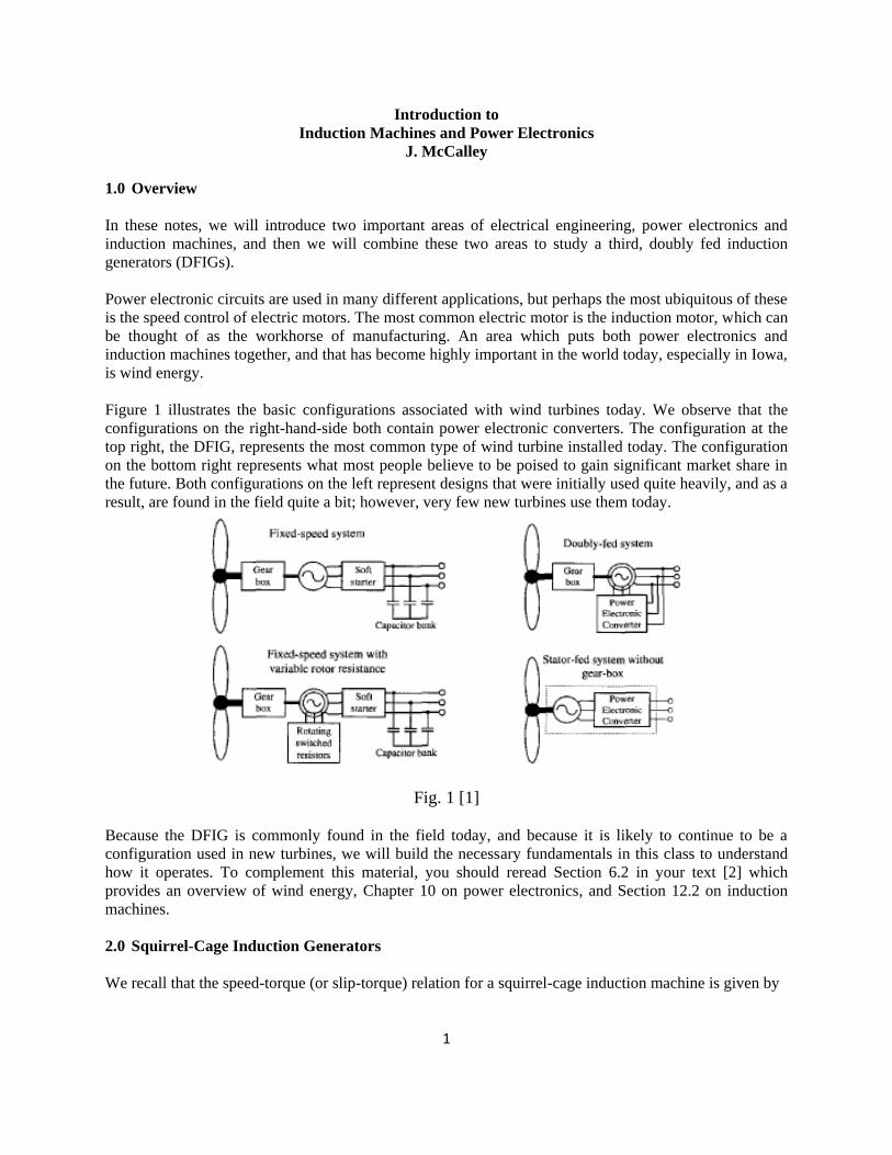
Figure 1 illustrates the basic configurations associated with wind turbines today. We observe that the
configurations on the right-hand-side both contain power electronic converters. The configuration at the
top right, the DFIG, represents the most common type of wind turbine installed today. The configuration
on the bottom right represents what most people believe to be poised to gain significant market share in
the future. Both configurations on the left represent designs that were initially used quite heavily, and as a
result, are found in the field quite a bit; however, very few new turbines use them today.
Fig. 1 [1]
Because the DFIG is commonly found in the field today, and because it is likely to continue to be a
configuration used in new turbines, we will build the necessary fundamentals in this class to understand
how it operates. To complement this material, you should reread Section 6.2 in your text [2] which
provides an overview of wind energy, Chapter 10 on power electronics, and Section 12.2 on induction
machines.
2.0 Squirrel-Cage Induction Generators
We recall that the speed-torque (or slip-torque) relation for a squirrel-cage induction machine is given by
2
2
2
222
2
3 '
''
th
s th th
V RT
Rs R X X
s
(1)
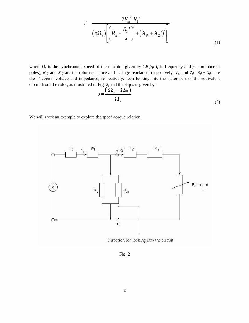
where Ωs is the synchronous speed of the machine given by 120f/p (f is frequency and p is number of
poles), R’2 and X’2 are the rotor resistance and leakage reactance, respectively, Vth and Zth=Rth+jXth are
the Thevenin voltage and impedance, respectively, seen looking into the stator part of the equivalent
circuit from the rotor, as illustrated in Fig. 2, and the slip s is given by
m
s=s
s
(2)
We will work an example to explore the speed-torque relation.
Fig. 2

3
Example: Consider a 6-pole induction generator with line-line voltage of 220 volts, and the below data.
Plot the torque-speed characteristic for f=60 Hz.
R1=0.294 Ω X’2=0.209 Ω
X1=0.503 Ω R’2=0.061 Ω
RC=1000 Ω
Xm=13.25 Ω
Solution: First we need to obtain ΩS. This is given by 2 / ( / 2) 2 (60) / (6 / 2) 125.664 / secs f p rad
We develop the speed-torque characteristic using the following Matlab code.
The above Matlab code results in the speed-torque relationship shown in Fig. 3. We observe here that
Motor operation is from Ωm=0 to Ωm= ΩS=125.664 rad/sec; reference to (1) shows this corresponds to
positive slip.
Generator operation is from Ωm=ΩS=125.664 rad/sec to Ωm=2ωS=251.328 rad/sec; reference to (1)
shows this corresponds to negative slip.
The developed torque for motor operation is positive and for generator operation is negative.
The maximum developed torque for motor operation is about half of the maximum developed torque
for generator operation. The reason for this can be seen in eq. (1) where the slip, when negative
(generator operation), results in a torque expression denominator that is smaller than when the slip is
positive (motor operation).
rth=real(zth);
xth=imag(zth);
% Mechanical speed range
wm1=[0*k*ws:1:2*k*ws];
% Torque equation components.
num=3*(vth^2)*rp2;
den1=ws*(1-wm1 /(k*ws));
den2=(rth+rp2./(1-wm1/(k*ws))).^2;
den3=(xth+xp2)^2;
% Compute torque
T1=num ./ (den1.*(den2+den3));
plot(wm1,T1)
grid
v1= 220/sqrt(3);
r1=0.294;
x1=0.503;
rc= 1000;
xm=13.25;
xp2=0.209;
rp2=0.0610;
ws=125.67;
% Compute thevenin
parameters.
zb=(rc*i*xm)/(rc+i*xm);
za=r1+i*x1;
vth=abs(v1*zb/(za+zb));
zth=za*zb/(za+zb);
This should be
denoted Ωs here and
then likewise in the
below matlab script.
4
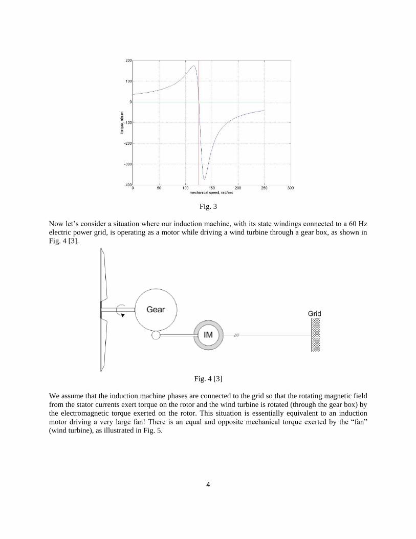
Fig. 3
Now let’s consider a situation where our induction machine, with its state windings connected to a 60 Hz
electric power grid, is operating as a motor while driving a wind turbine through a gear box, as shown in
Fig. 4 [3].
Fig. 4 [3]
We assume that the induction machine phases are connected to the grid so that the rotating magnetic field
from the stator currents exert torque on the rotor and the wind turbine is rotated (through the gear box) by
the electromagnetic torque exerted on the rotor. This situation is essentially equivalent to an induction
motor driving a very large fan! There is an equal and opposite mechanical torque exerted by the “fan”
(wind turbine), as illustrated in Fig. 5.
5
Fig. 5
Let’s assume that the speed-torque characteristic of the “fan” is as in Fig. 6, which means that the
equilibrium point (the steady-state operating point) is the intersection of the two speed-torque
characteristics.
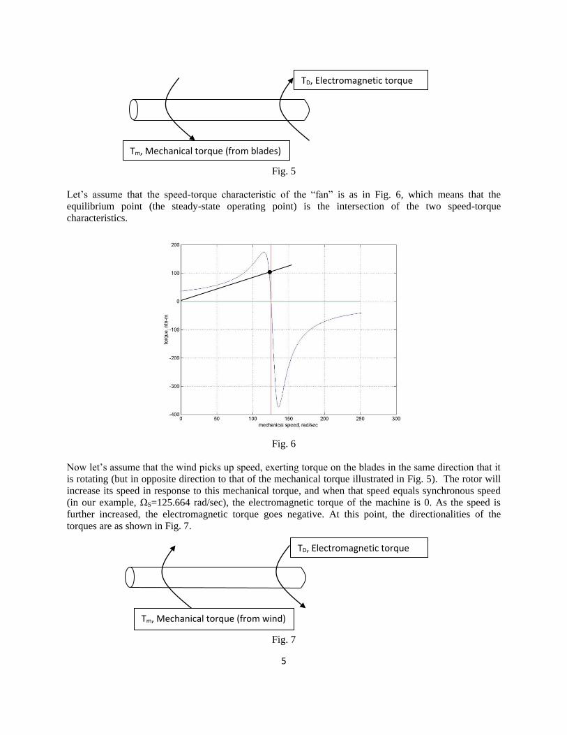
Fig. 6
Now let’s assume that the wind picks up speed, exerting torque on the blades in the same direction that it
is rotating (but in opposite direction to that of the mechanical torque illustrated in Fig. 5). The rotor will
increase its speed in response to this mechanical torque, and when that speed equals synchronous speed
(in our example, ΩS=125.664 rad/sec), the electromagnetic torque of the machine is 0. As the speed is
further increased, the electromagnetic torque goes negative. At this point, the directionalities of the
torques are as shown in Fig. 7.
Fig. 7
TD, Electromagnetic torque
Tm, Mechanical torque (from wind)
TD, Electromagnetic torque
Tm, Mechanical torque (from blades)
6
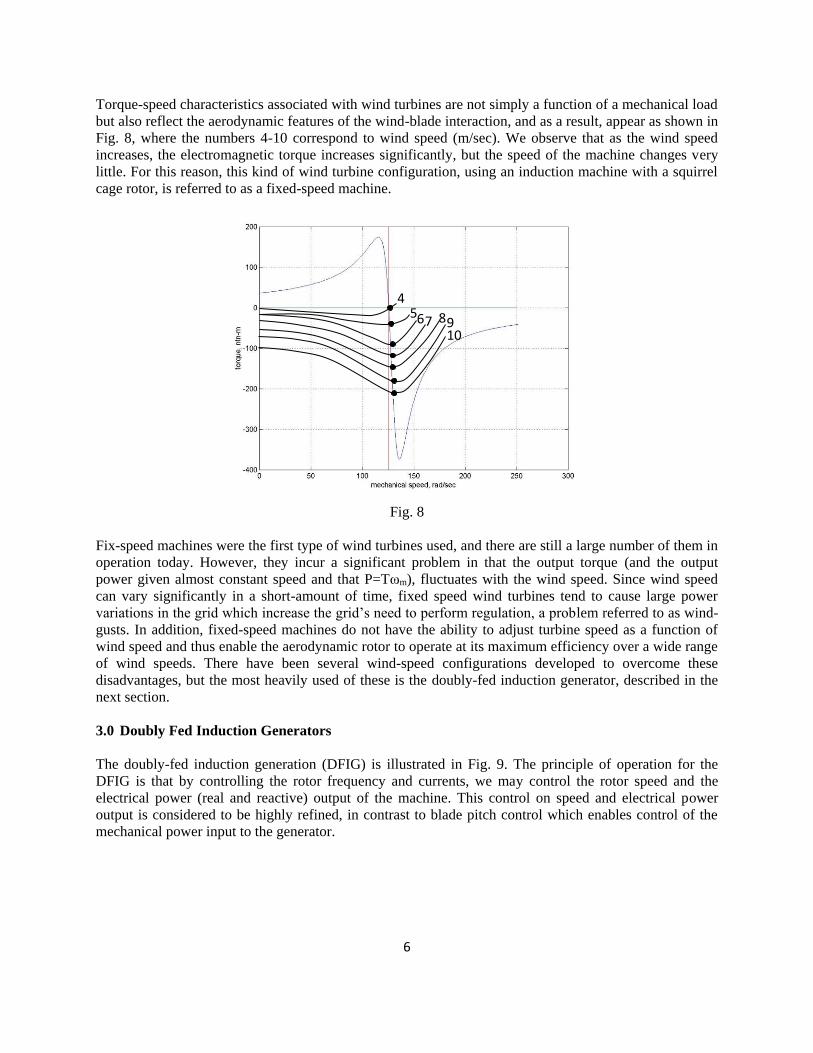
Torque-speed characteristics associated with wind turbines are not simply a function of a mechanical load
but also reflect the aerodynamic features of the wind-blade interaction, and as a result, appear as shown in
Fig. 8, where the numbers 4-10 correspond to wind speed (m/sec). We observe that as the wind speed
increases, the electromagnetic torque increases significantly, but the speed of the machine changes very
little. For this reason, this kind of wind turbine configuration, using an induction machine with a squirrel
cage rotor, is referred to as a fixed-speed machine.
Fig. 8
Fix-speed machines were the first type of wind turbines used, and there are still a large number of them in
operation today. However, they incur a significant problem in that the output torque (and the output
power given almost constant speed and that P=Tωm), fluctuates with the wind speed. Since wind speed
can vary significantly in a short-amount of time, fixed speed wind turbines tend to cause large power
variations in the grid which increase the grid’s need to perform regulation, a problem referred to as wind-
gusts. In addition, fixed-speed machines do not have the ability to adjust turbine speed as a function of
wind speed and thus enable the aerodynamic rotor to operate at its maximum efficiency over a wide range
of wind speeds. There have been several wind-speed configurations developed to overcome these
disadvantages, but the most heavily used of these is the doubly-fed induction generator, described in the
next section.
3.0 Doubly Fed Induction Generators
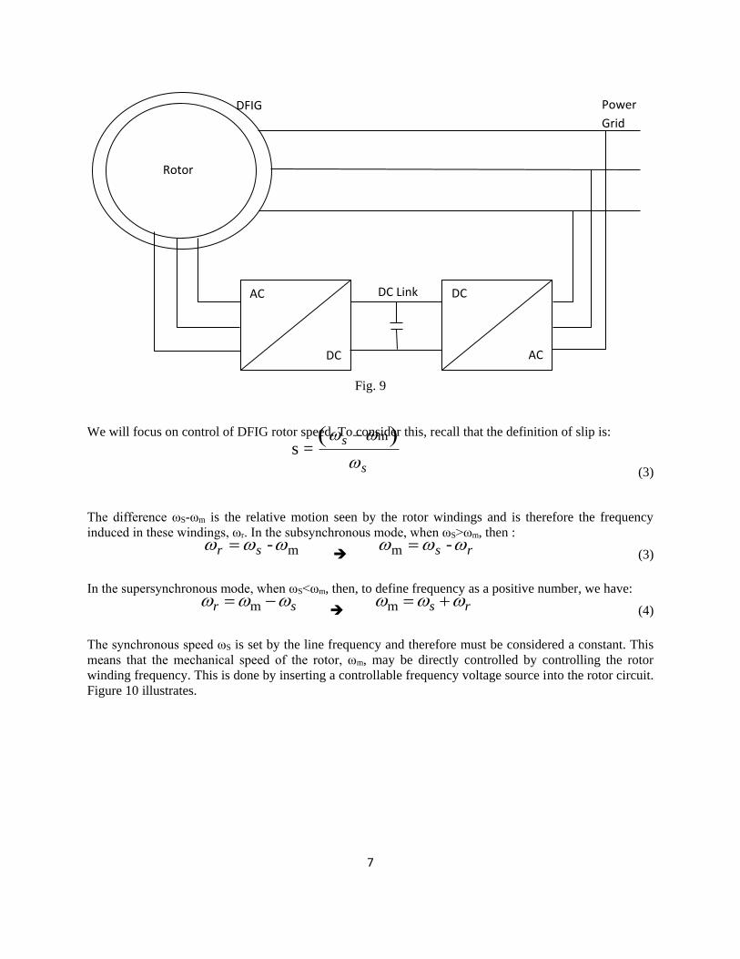
The doubly-fed induction generation (DFIG) is illustrated in Fig. 9. The principle of operation for the
DFIG is that by controlling the rotor frequency and currents, we may control the rotor speed and the
electrical power (real and reactive) output of the machine. This control on speed and electrical power
output is considered to be highly refined, in contrast to blade pitch control which enables control of the
mechanical power input to the generator.
4 5 6 7 8 9
10
7
Fig. 9
We will focus on control of DFIG rotor speed. To consider this, recall that the definition of slip is:
s
s
m=s
(3)
The difference ωS-ωm is the relative motion seen by the rotor windings and is therefore the frequency
induced in these windings, ωr. In the subsynchronous mode, when ωS>ωm, then :
m- sr
rs -m (3)
In the supersynchronous mode, when ωS<ωm, then, to define frequency as a positive number, we have:
sr m
rs m (4)
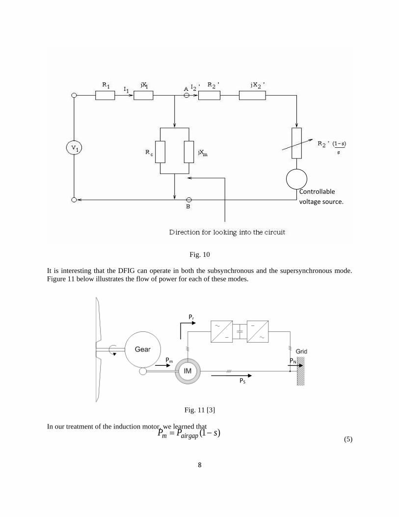
The synchronous speed ωS is set by the line frequency and therefore must be considered a constant. This
means that the mechanical speed of the rotor, ωm, may be directly controlled by controlling the rotor
winding frequency. This is done by inserting a controllable frequency voltage source into the rotor circuit.
Figure 10 illustrates.
AC
DC
DC
AC
DFIG
Rotor
Power
Grid
DC Link
8
Fig. 10
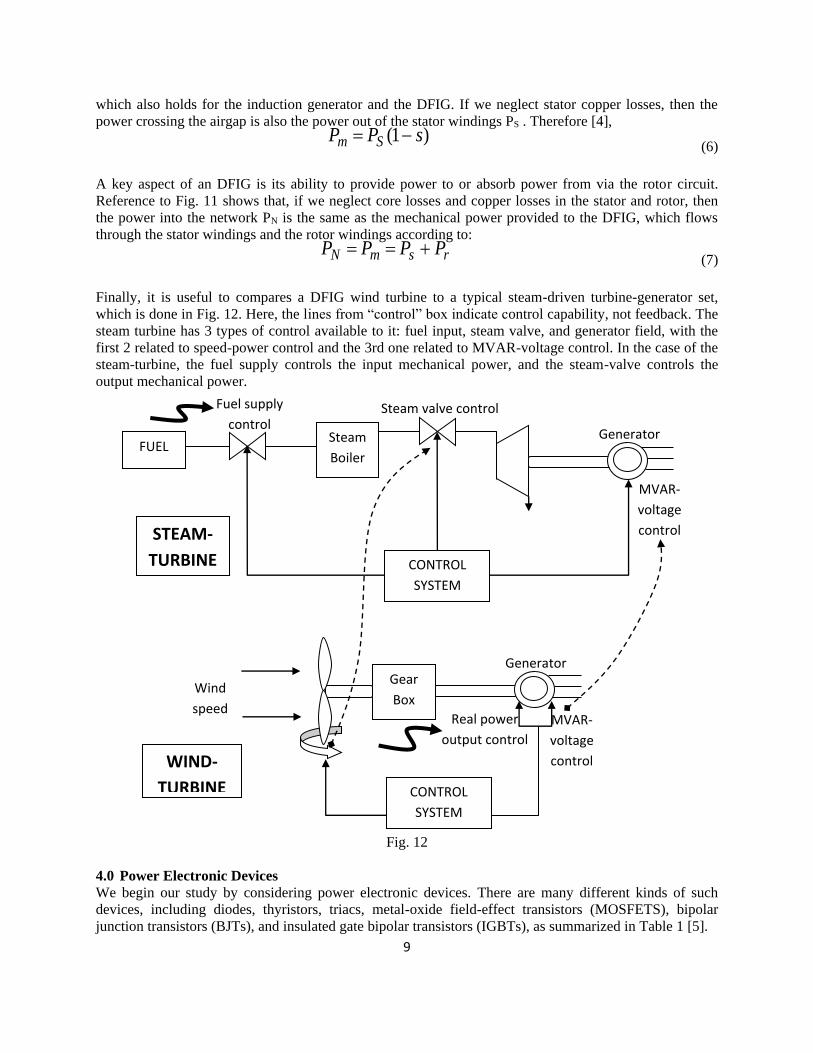
It is interesting that the DFIG can operate in both the subsynchronous and the supersynchronous mode.
Figure 11 below illustrates the flow of power for each of these modes.
Fig. 11 [3]
In our treatment of the induction motor, we learned that )1( sPP airgapm (5)
PS
Pr
Pm PN
Controllable
voltage source.
9
which also holds for the induction generator and the DFIG. If we neglect stator copper losses, then the
power crossing the airgap is also the power out of the stator windings PS . Therefore [4],
)1( sPP Sm (6)
A key aspect of an DFIG is its ability to provide power to or absorb power from via the rotor circuit.
Reference to Fig. 11 shows that, if we neglect core losses and copper losses in the stator and rotor, then
the power into the network PN is the same as the mechanical power provided to the DFIG, which flows
through the stator windings and the rotor windings according to:
rsmN PPPP (7)
Finally, it is useful to compares a DFIG wind turbine to a typical steam-driven turbine-generator set,
which is done in Fig. 12. Here, the lines from “control” box indicate control capability, not feedback. The
steam turbine has 3 types of control available to it: fuel input, steam valve, and generator field, with the
first 2 related to speed-power control and the 3rd one related to MVAR-voltage control. In the case of the
steam-turbine, the fuel supply controls the input mechanical power, and the steam-valve controls the
output mechanical power.
Fig. 12
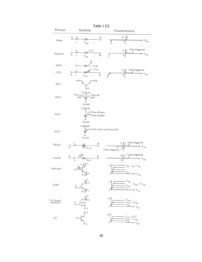
4.0 Power Electronic Devices
We begin our study by considering power electronic devices. There are many different kinds of such
devices, including diodes, thyristors, triacs, metal-oxide field-effect transistors (MOSFETS), bipolar
junction transistors (BJTs), and insulated gate bipolar transistors (IGBTs), as summarized in Table 1 [5].
FUEL Steam
Boiler
Generator
CONTROL
SYSTEM
Steam valve control Fuel supply
control
MVAR-
voltage
control
Wind
speed
Gear
Box
Generator
CONTROL
SYSTEM
MVAR-
voltage
control
Real power
output control
STEAM-
TURBINE
WIND-
TURBINE
10
Table 1 [5]
11
All of them, however, have a common operating behavior when used in power electronic circuits: they are
switches! We describe operating characteristics of a few of them in what follows.
4.1 BJTs
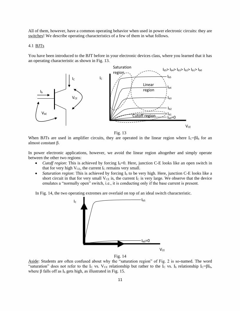
You have been introduced to the BJT before in your electronic devices class, where you learned that it has
an operating characteristic as shown in Fig. 13.
Fig. 13
When BJTs are used in amplifier circuits, they are operated in the linear region where IC=βIb for an
almost constant β.
In power electronic applications, however, we avoid the linear region altogether and simply operate
between the other two regions:
Cutoff region: This is achieved by forcing Ib=0. Here, junction C-E looks like an open switch in
that for very high VCE, the current IC remains very small.
Saturation region: This is achieved by forcing Ib to be very high. Here, junction C-E looks like a
short circuit in that for very small VCE is, the current IC is very large. We observe that the device
emulates a “normally open” switch, i.e., it is conducting only if the base current is present.
In Fig. 14, the two operating extremes are overlaid on top of an ideal switch characteristic.
Fig. 14
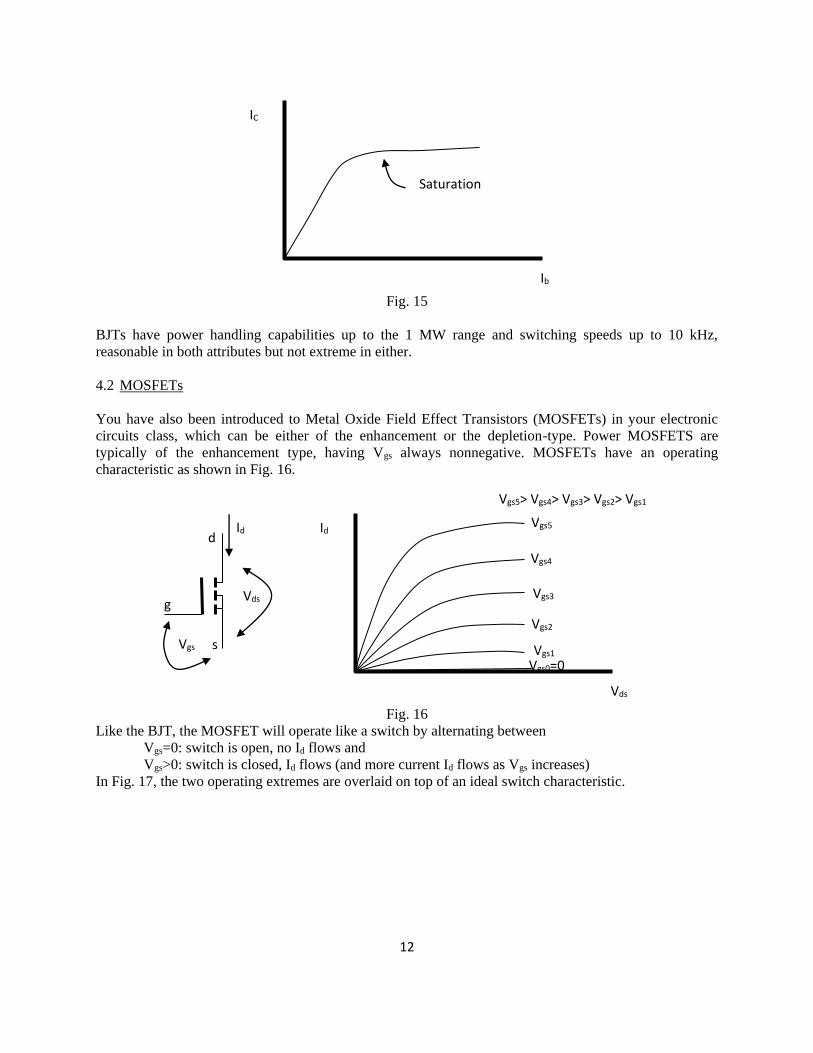
Aside: Students are often confused about why the “saturation region” of Fig. 2 is so-named. The word
“saturation” does not refer to the IC vs. VCE relationship but rather to the IC vs. Ib relationship IC=βIb,
where β falls off as Ib gets high, as illustrated in Fig. 15.
IC
VCE
Ib5
Ib0=0
IC
VCE
Ib5
Ib4
Ib3
Ib2
Ib1 Ib0=0
Saturation region
Ib
IC
VCE
VbE
Ib5> Ib4> Ib3> Ib2> Ib1> Ib0
Linear region
Cutoff region
12
Fig. 15
BJTs have power handling capabilities up to the 1 MW range and switching speeds up to 10 kHz,
reasonable in both attributes but not extreme in either.
4.2 MOSFETs
You have also been introduced to Metal Oxide Field Effect Transistors (MOSFETs) in your electronic
circuits class, which can be either of the enhancement or the depletion-type. Power MOSFETS are
typically of the enhancement type, having Vgs always nonnegative. MOSFETs have an operating
characteristic as shown in Fig. 16.
Fig. 16
Like the BJT, the MOSFET will operate like a switch by alternating between
Vgs=0: switch is open, no Id flows and
Vgs>0: switch is closed, Id flows (and more current Id flows as Vgs increases)
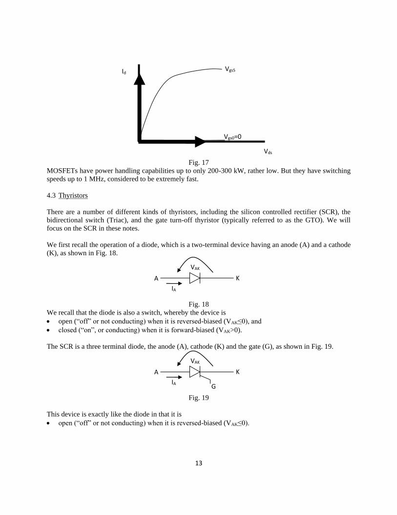
In Fig. 17, the two operating extremes are overlaid on top of an ideal switch characteristic.
Id
Vds
Vgs5
Vgs4
Vgs3
Vgs2
Vgs1
Id
Vds
Vgs
Vgs5> Vgs4> Vgs3> Vgs2> Vgs1
g
s
d
Vgs0=0
IC
Ib
Saturation
13
Fig. 17
MOSFETs have power handling capabilities up to only 200-300 kW, rather low. But they have switching
speeds up to 1 MHz, considered to be extremely fast.
4.3 Thyristors
There are a number of different kinds of thyristors, including the silicon controlled rectifier (SCR), the
bidirectional switch (Triac), and the gate turn-off thyristor (typically referred to as the GTO). We will
focus on the SCR in these notes.
We first recall the operation of a diode, which is a two-terminal device having an anode (A) and a cathode
(K), as shown in Fig. 18.
Fig. 18
We recall that the diode is also a switch, whereby the device is
open (“off” or not conducting) when it is reversed-biased (VAK≤0), and
closed (“on”, or conducting) when it is forward-biased (VAK>0).
The SCR is a three terminal diode, the anode (A), cathode (K) and the gate (G), as shown in Fig. 19.
Fig. 19
This device is exactly like the diode in that it is
open (“off” or not conducting) when it is reversed-biased (VAK≤0).
A K
VAK
IA G
Id
Vds
Vgs5
Vgs0=0
A K
VAK
IA
14
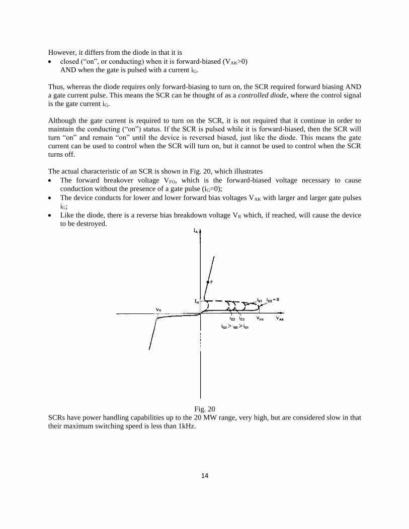
However, it differs from the diode in that it is
closed (“on”, or conducting) when it is forward-biased (VAK>0)
AND when the gate is pulsed with a current iG.
Thus, whereas the diode requires only forward-biasing to turn on, the SCR required forward biasing AND
a gate current pulse. This means the SCR can be thought of as a controlled diode, where the control signal
is the gate current iG.
Although the gate current is required to turn on the SCR, it is not required that it continue in order to
maintain the conducting (“on”) status. If the SCR is pulsed while it is forward-biased, then the SCR will
turn “on” and remain “on” until the device is reversed biased, just like the diode. This means the gate
current can be used to control when the SCR will turn on, but it cannot be used to control when the SCR
turns off.
The actual characteristic of an SCR is shown in Fig. 20, which illustrates
The forward breakover voltage VFO, which is the forward-biased voltage necessary to cause
conduction without the presence of a gate pulse (iG=0);
The device conducts for lower and lower forward bias voltages VAK with larger and larger gate pulses
iG;
Like the diode, there is a reverse bias breakdown voltage VR which, if reached, will cause the device
to be destroyed.
Fig. 20
SCRs have power handling capabilities up to the 20 MW range, very high, but are considered slow in that
their maximum switching speed is less than 1kHz.
15
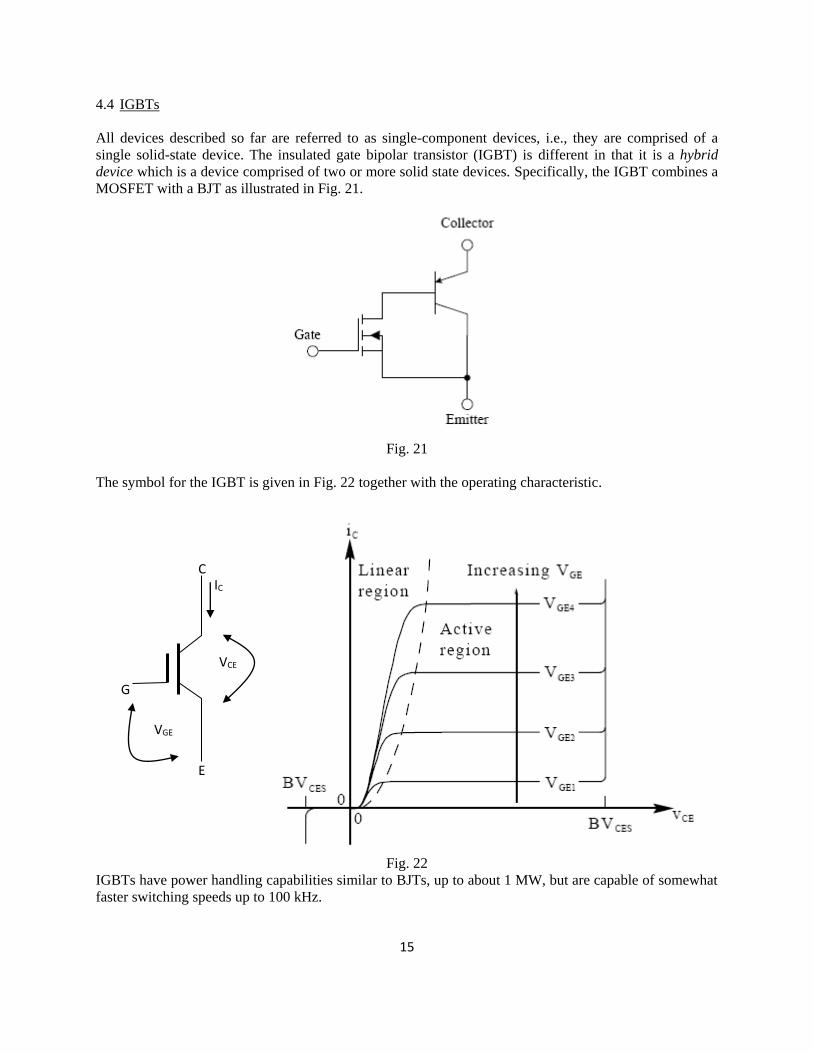
4.4 IGBTs
All devices described so far are referred to as single-component devices, i.e., they are comprised of a
single solid-state device. The insulated gate bipolar transistor (IGBT) is different in that it is a hybrid
device which is a device comprised of two or more solid state devices. Specifically, the IGBT combines a
MOSFET with a BJT as illustrated in Fig. 21.
Fig. 21
The symbol for the IGBT is given in Fig. 22 together with the operating characteristic.
Fig. 22
IGBTs have power handling capabilities similar to BJTs, up to about 1 MW, but are capable of somewhat
faster switching speeds up to 100 kHz.
C
E
G
IC
VGE
VCE

16
4.5 Device ratings
Key distinguishing characteristics between power electronic devices are the speed at which they can
switch, measured in Hz, and their power handling capabilities, which are a function of their voltage and
current ratings. We have provided numerical ranges associated with these attributes for each device
discussed so far. Figure 23 [] provides an effective way to compare some of these different devices in
these terms.
Fig. 23
The switching time is comprised of the turn-on time and the turn-off time. The turn-on time, ton, is the
interval between applying the triggering gate pulse and device turn-on. The turn-off time, tq, is the time
required after forward current has ceased before forward voltage may again be applied without turn-on.
The maximum switching frequency is then given by 1/(ton+tq).
There are some other device ratings of importance, including the following:
Voltage breakdown: This is the maximum reverse bias voltage that can be applied on an “off-state”
beyond which the device breaks down and is damaged.
Current rating: This is the maximum current the device can carry beyond which excessive heating
within the device destroys it.
Maximum di/dt: Some time is necessary during device turn-on for the current to spread uniformly
across the junction, and if di/dt is too large, the current flows in too small a region of the junction,
causing high current density, excessive localized heating (a hot spot), and device failure.
Maximum dv/dt: Excessive dv/dt causes a device to turn off.
4.5.1 Limiting di/dt
4.5.2 Limiting dv/dt

17
5.0 Power electronic converters
We are well aware that our electric energy is delivered to us via AC systems. However, there are some
DC applications, including, for example, DC motors, where we must convert AC into DC in order to
supply these devices from the AC grid. There are also DC sources, including, for example, solar cells and
wind turbines with DC generators, where we must convert DC to AC in order to integrate these devices
into the AC grid. There are also DC transmission lines that are embedded within the AC grid which
require the AC to be converted to DC at the sending end and the DC to be converted back to AC at the
receiving end.
Finally, there are control applications where it is useful to convert AC to AC in order to exert control over
a device. The control may be in terms of voltage, frequency, or both. A light dimmer is a very common
device which converts AC to AC for control of the power that is supplied to a light bulb, thus varying its
luminosity. A device which does both is called the cycloconverter, used to control motors which convert
rotational motion to linear motion (so-called traction motors), as is common in rail applications. The
power electronic application of interest to us here is for AC to AC control of the frequency of the
induction motor rotor currents. It is illustrated in Fig. 9.
In general, power electronic circuits which convert from one power type to another are called converters.
There are other names used for specific kinds of converters, as follows:
AC to DC: rectifiers
DC to AC: inverters
DC to DC: choppers (also switching regulators)
AC to AC: converters (also voltage controllers, frequency changers, or cycloconverters)
We will focus on the AC to DC rectifiers in what follows and then show how study each of these in what
follows.
5.1 AC to DC
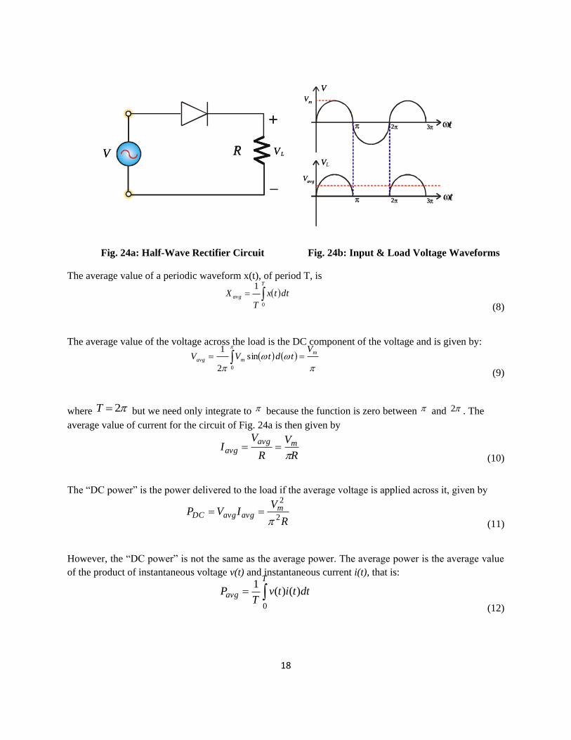
Half-wave rectifier:
A simple diode half-wave rectifier consists of an alternating voltage source in series with a diode and a
resistor as shown in Fig. 24a. During the positive half cycle ( t 0 ), the diode conducts and the
current flows through the load resistance R. During the negative half-cycle ( 2t ), the diode is off
and acts like an open switch. Figure 24b shows the resulting waveforms for a sinusoidal input voltage
source of tVv m sin .
18
L V R V
m V V
2 3 t
t
avg V
V
2 3
L V V
m V V
2 3
avg V
VL
2 3
Fig. 24a: Half-Wave Rectifier Circuit Fig. 24b: Input & Load Voltage Waveforms
The average value of a periodic waveform x(t), of period T, is
T
avg dttx
T
X0
1
(8)
The average value of the voltage across the load is the DC component of the voltage and is given by:
m
mavg
VtdtVV
0
sin
2
1
(9)
where 2T but we need only integrate to because the function is zero between and 2 . The
average value of current for the circuit of Fig. 24a is then given by
R
V
R
VI mavg
avg
(10)
The “DC power” is the power delivered to the load if the average voltage is applied across it, given by
R
VIVP m
avgavgDC 2
2
(11)
However, the “DC power” is not the same as the average power. The average power is the average value
of the product of instantaneous voltage v(t) and instantaneous current i(t), that is:
T
avg dttitvT
P
0
)()(1
(12)
19
The average power may be obtained by taking the product of the RMS voltage and current. For a voltage
or current having a purely sinusoidal waveform, the RMS value will be 0.707 multiplied by the peak
value. For a voltage or current having a non-sinusoidal waveform, the RMS value must be obtained by
taking the root-mean square of the waveform over one period.
For the half wave rectifier circuit of Fig. 24a, the RMS value of the voltage across the load is
2
sin2
1
0
2 mmrms
VtdtVV
(13)
The RMS current is then given by
R
V
R
VI mrms
rms2
(14)
The average power is then given by
R
VIVP m
rmsrmsavg4
2
(15)
We observe that the average power is greater than the “DC power” for a purely resistive circuit by a
factor of
4674.24
42
2
2
2
R
V
R
V
P
P
m
m
DC
avg
(16)
Therefore, computing power must be done with RMS quantities. Although DC quantities for voltages and
currents are often obtained for power electronic circuits, their use for power calculations should always be
seen to be approximations at best [6, pg. 40]. Two other ways to compute power that are of interest when
either one or both waveforms are nonsinusoidal include [6, pp. 37-40] (a) taking the average of the
product of instantaneous voltage and current; and (b) taking a Fourier series of voltage and current and
then adding products of like harmonics.
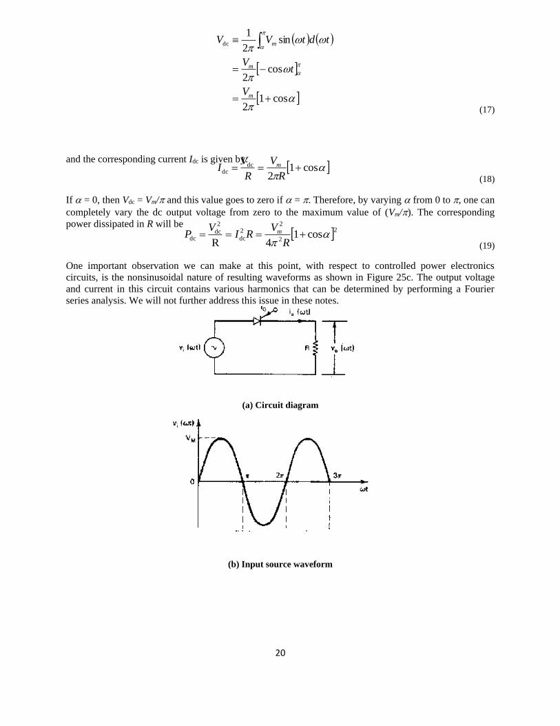
Controlled Half-wave rectifier:
A simple form of a controlled half-wave rectifier feeding a resistive load, such as an electric heater or
incandescent lamp, is shown in Fig. 25a. If the input source tVtv mi sin
is as drawn in Fig. 25b,
the corresponding output voltage and the resulting current wave are as indicated in Fig. 25c for a
particular triggering (firing) angle . The anode-cathode voltage across the thyristor is depicted in Fig.
25d. The triggering current pulse of suitable magnitude and duration required to turn on the SCR at t =
is shown in Figure 25e. If = 0, we realize an uncontrolled half-wave rectifier employing a diode. For
this scheme, the average value of the output voltage Vdc is:
20
cos12
cos2
sin2
1dc
m
m
m
V
tV
tdtVV
(17)
and the corresponding current Idc is given by:
cos1
2
dcdc
R
V
R
VI m
(18)
If = 0, then Vdc = Vm/ and this value goes to zero if = . Therefore, by varying from 0 to , one can
completely vary the dc output voltage from zero to the maximum value of (Vm/). The corresponding
power dissipated in R will be 2
2
22
dc
2
dcdc cos1
4R
R
VRI
VP m
(19)
One important observation we can make at this point, with respect to controlled power electronics
circuits, is the nonsinusoidal nature of resulting waveforms as shown in Figure 25c. The output voltage
and current in this circuit contains various harmonics that can be determined by performing a Fourier
series analysis. We will not further address this issue in these notes.
(a) Circuit diagram
(b) Input source waveform
21
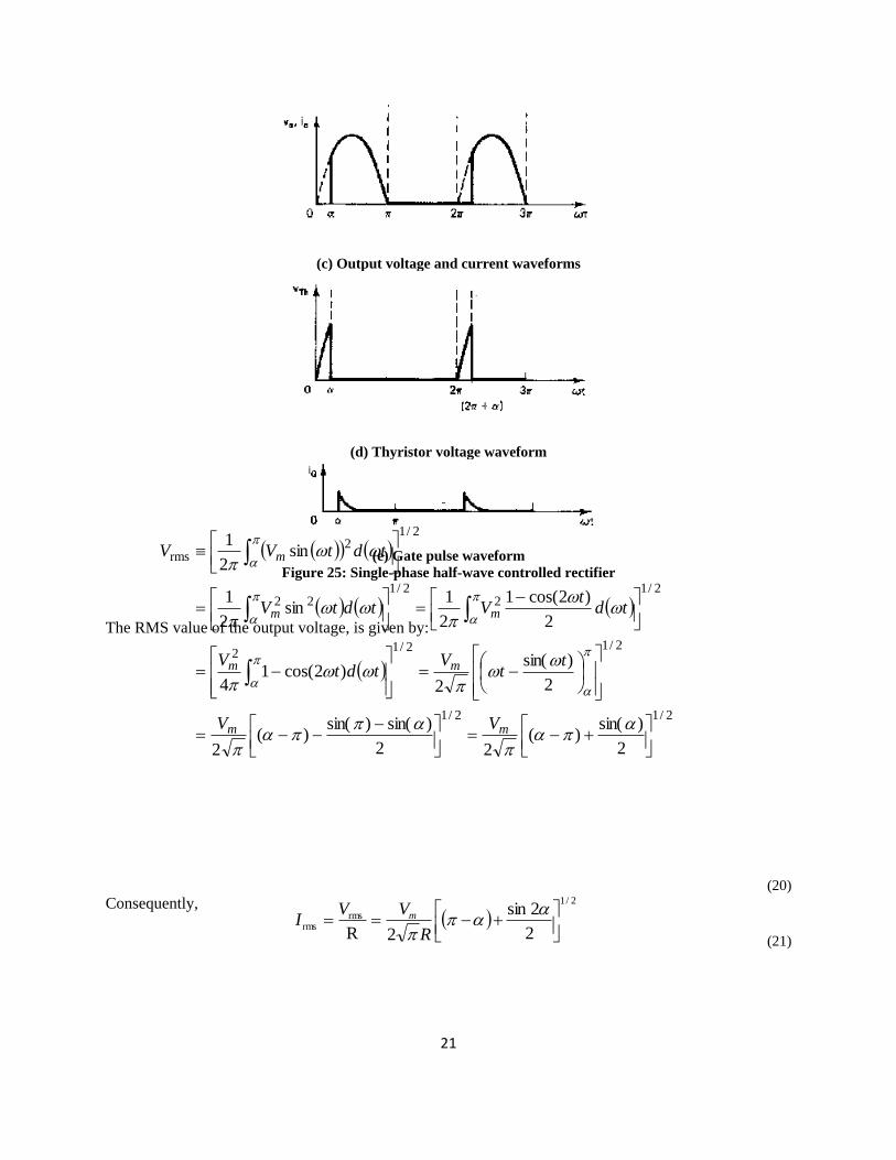
(c) Output voltage and current waveforms
(d) Thyristor voltage waveform
(e) Gate pulse waveform
Figure 25: Single-phase half-wave controlled rectifier
The RMS value of the output voltage, is given by:
2/12/1
2/12/12
2/12
2/122
2/12
rms
2
)sin()(
22
)sin()sin()(
2
2
)sin(
2)2cos(1
4
2
)2cos(1
2
1sin
2
1
sin2
1
mm
mm
mm
m
VV
tt
Vtdt
V
tdt
VtdtV
tdtVV
(20)
Consequently,
2/1
rmsrms
2
2sin
2R
R
VVI m
(21)

22
We now define a measure called Ripple Factor (r) for quantifying the smoothness of the output voltage. 100 of components ac all of valuerms
%dc
0 V
vr
(22)
This can be shown to reduce to: 1001001
2dc
2rms
2/1
2dc
2rms
dcV
VV
V
Vr
(23)
Full wave rectifier:
The full wave rectifier is described in Module PE1 of your notes.
Three phase rectifier:
The single-phase, full-wave bridge scheme can be extended to accommodate a three-phase input source.
Most popular and versatile is the 6-pulse converter, or controlled rectifier. Prior to the invention of
thyristors, mercury arc rectifiers were employed to realize controlled rectification. The well-known
Pacific 500 kV, HVDC transmission line linking the northwest region at Celilo, Oregon, to Sylmar, near
Los Angeles in the southwest region, adopted the mercury arc rectifiers. We will explore this important
application later in this section after gaining an understanding of this converter scheme.
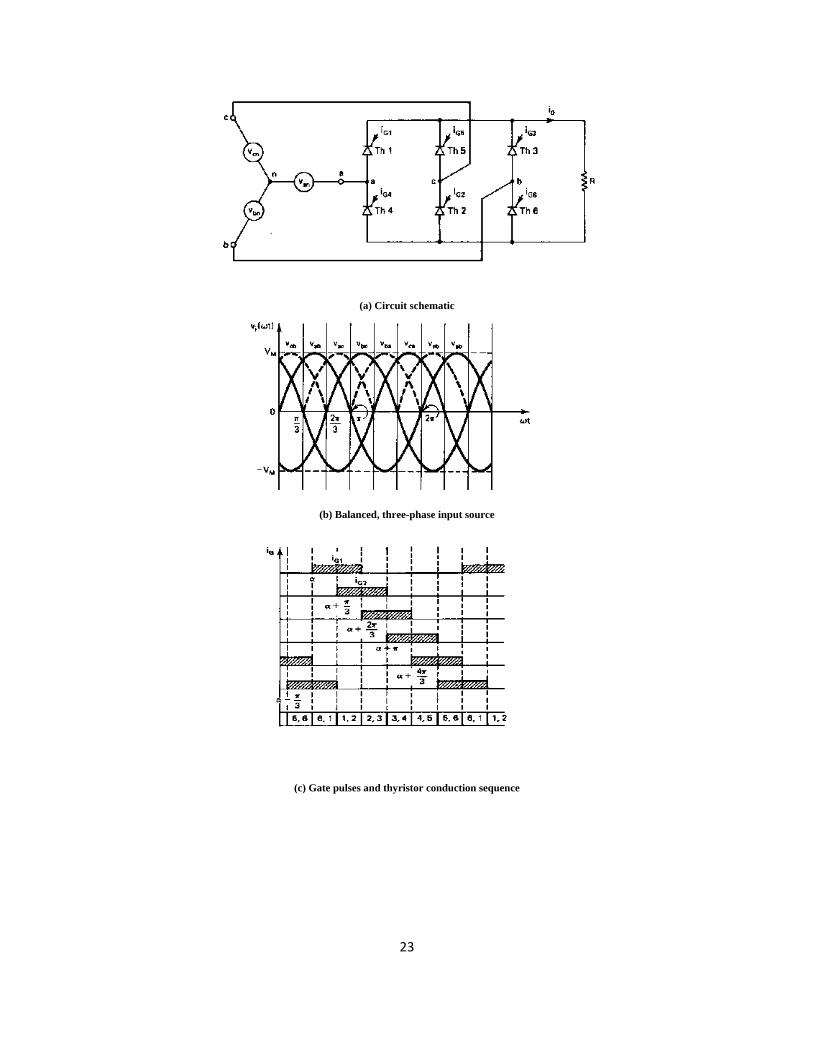
The circuit of Fig. 25 employs a Y-connected, three-phase source vi(t), delivering dc output vo(t) to
resistive load through a thyristor bridge consisting of six controlled switches; hence it is called a 6-pulse
converter.
The operation of the scheme can be understood based on the following observations:
1. Exactly two SCRs are conducting at any moment, as can be seen from the bottom of Fig. 26c.
One SCR is fired at α= ωt and then left on for 60°, after which an SCR is fired every 60° thereafter.
We turn on the pair of SCRs that give the most positive line-to-line voltage. We can determine the
SCR pair that should be on by (a) identifying the most positive line-to-line voltage; (b) inspecting
the circuit and identifying how to place the most positive line-to-line voltage across the load.
2. Thyristors turn off when they become reversed biased. This occurs whenever the voltage applied at
their cathode exceeds the voltage applied at their anode.
For the time period t=0 to /3,
vcb is the most positive voltage relative to other line-to-line voltages;
Th 5, 6 conduct if suitable pulses are applied, or are already applied, to their respective gates;
at the end of the time period, at t=/3, we turn on Th 1 to apply vab across the load;
Although Th5 is on at t=/3, vab goes higher than vcb at that moment, which reverse biases Th 5, and
it commutates (turns off).
For the time period t = /3 to 2/3,
vab is the most positive voltage relative to other line-to-line voltages;
Th 1, 6 conduct if suitable pulses are applied, or are already applied, to their respective gates;
at the end of the time period, at t=2/3, we turn on Th 2 to apply vac across the load;
Although Th6 is on at t=2/3, vac goes higher than vab at that moment, which reverse biases Th 6,
and it commutates (turns off).
23
(a) Circuit schematic
(b) Balanced, three-phase input source
(c) Gate pulses and thyristor conduction sequence
24
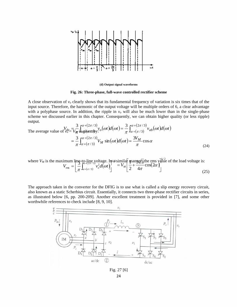
(d) Output signal waveforms
Fig. 26: Three-phase, full-wave controlled rectifier scheme
A close observation of vo clearly shows that its fundamental frequency of variation is six times that of the
input source. Therefore, the harmonic of the output voltage will be multiple orders of 6, a clear advantage
with a polyphase source. In addition, the ripple in vo will also be much lower than in the single-phase
scheme we discussed earlier in this chapter. Consequently, we can obtain higher quality (or less ripple)
output.
The average value of vo = Vdc is given by:
cos3
sin3
33
3/2
3/
3/2
3/
3/2
3/dc
MM
abo
VtdtV
tdtvtdtvV
(24)
where VM is the maximum line-to-line voltage. In a similar manner, the rms value of the load voltage is:
2/1
3/2
3/
2
rms
3
tdvV o
2/1
2cos4
33
2
1
MV
(25)
The approach taken in the converter for the DFIG is to use what is called a slip energy recovery circuit,
also known as a static Scherbius circuit. Essentially, it connects two three-phase rectifier circuits in series,
as illustrated below [6, pp. 200-209]. Another excellent treatment is provided in [7], and some other
worthwhile references to check include [8, 9, 10].
Fig. 27 [6]

25
Some other issues to address:
Operation of the DC to AC link, PWM.
Ability for power to flow through the converter in both directions.
Functionality of the DC link, with inductor, and with capacitor.
Definition of the voltage source converter.
5.2 DC to AC
5.3 DC to DC
5.4 AC to AC
[1] T. Thiringer, A. Petersson and T. Petru, “Grid Disturbance Response of Wind Turbines Equipped with Induction
Generator and Doubly-Fed Induction Generator,” 2003.
[2] M. El Sharkawi, “Electric Energy: An Introduction,” second edition, CRC Press, 2008.
[3] S. Soter and R. Wegener, “Development of Induction Machines in Wind Power Technology,” available at
http://www-mal.e-technik.uni-dortmund.de/paper/upload/paper_71.pdf.
[4] B. Fox, et al., “Wind Power Integration: Connection and System Operational Aspects,” Institution of
Engineering and Technology, UK, 2007, pp. 73-75, available at
http://books.google.com/books?id=LTuo24RfTGoC&pg=PR6&lpg=PR6&dq=%22Induction+generator%22+%22fi
xed-speed%22+%22energy+extraction%22&source=bl&ots=H6HqFRz2fI&sig=ILiL_n-
bEoOMJyOjTW7bzWwebGI&hl=en&ei=6MLVS7zPDsO88gbQkqHlDw&sa=X&oi=book_result&ct=result&resnu
m=4&ved=0CBgQ6AEwAzgU#v=onepage&q=%22Induction%20generator%22%20%22fixed-
speed%22%20%22energy%20extraction%22&f=false.
[5] M. Rashid, “Power electronics: Circuits, Devices, and Applications,” second edition, Prentice-Hall, 1993.
[6] M. El-Sharkawi, “Fundamentals of Electric Drives,” Brooks/Cole Publishing, 2000.
[7] I. Boldea, “Variable Speed Generators,” Taylor & Francis, 2006.
[8] I. Boldea and S. Nasar, “The Induction Machine Handbook,” CRC Press, 2000.
[9] S. Heier, “Grid Integration of Wind Energy Conversion Systems,” Wiley, 1998.
[10] M. Stiebler, “Wind Energy Systems for Electric Power Generation,” Springer, 2008.
Recommended