Copyright© Biological and Agricultural Engineering Department, Texas A&M University1
Introduction to Load Duration Curves
Lucas GregoryTexas Water Resources Institute
Kyna McKeeR. KarthikeyanBiological and Agricultural EngineeringTexas A&M University
Copyright© Biological and Agricultural Engineering Department, Texas A&M University2
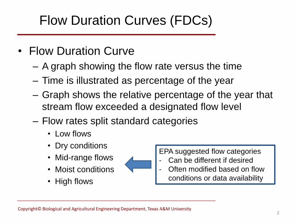
Flow Duration Curves (FDCs)
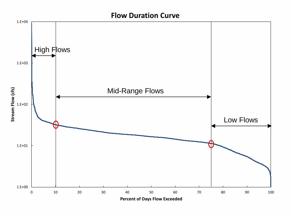
• Flow Duration Curve
– A graph showing the flow rate versus the time
– Time is illustrated as percentage of the year
– Graph shows the relative percentage of the year that
stream flow exceeded a designated flow level
– Flow rates split standard categories
• Low flows
• Dry conditions
• Mid-range flows
• Moist conditions
• High flows
EPA suggested flow categories
- Can be different if desired
- Often modified based on flow
conditions or data availability

Copyright© Biological and Agricultural Engineering Department, Texas A&M University3
Flow Duration Curve: Flow categories
• Can be the standard flow categories– High flows: 0 to 10% exceedance
– Moist conditions: 10 to 40% exceedance
– Mid-range flows: 40 to 60% exceedance
– Dry conditions: 60 to 90% exceedance
– Low flows: 90 to 100% exceedance
• Can develop your own flow categories based on the flow duration curve– Measured or simulated daily stream flow data over multiple
years is preferred
– Intermittent instantaneous data also works
– Create flow breaks based on change in slope in FDC graph
1.E+00
1.E+01
1.E+02
1.E+03
1.E+04
0 10 20 30 40 50 60 70 80 90 100
Stre
am F
low
(cf
s)
Percent of Days Flow Exceeded
Flow Duration Curve
Low Flows
High Flows
Mid-Range Flows

Copyright© Biological and Agricultural Engineering Department, Texas A&M University5
Load Duration Curves (LDCs)
• Load Duration Curve
– Combines concentrations of a pollutant with flow at
the same time to develop a load
– The LDC illustrates the load of a pollutant versus the
time that a given load is exceeded
– Time is illustrated as percentage of the year
– Able to see if a stream is exceeding the standard in
terms of load (flow and concentration)
– Able to calculate a percent reduction based on flow
categories

Load Duration Curve
1.E+08
1.E+09
1.E+10
1.E+11
1.E+12
1.E+13
0 10 20 30 40 50 60 70 80 90 100
Percent of Days Load Exceeded
Da
ily
Av
era
ge
Lo
ad
s
(cfu
/da
y)
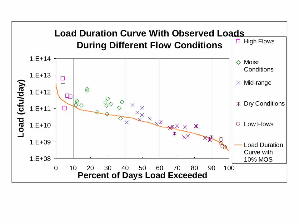
Load Duration Curve With Observed Loads
During Different Flow Conditions
1.E+08
1.E+09
1.E+10
1.E+11
1.E+12
1.E+13
1.E+14
0 10 20 30 40 50 60 70 80 90 100
Percent of Days Load Exceeded
Lo
ad
(cfu
/day)
High Flows
MoistConditions
Mid-range
Dry Conditions
Low Flows
Load DurationCurve with10% MOS

Load Regression Model on Load Duration Curve
Plot
1.E+08
1.E+09
1.E+10
1.E+11
1.E+12
1.E+13
1.E+14
0 10 20 30 40 50 60 70 80 90 100
Percent of Days Load Exceeded
Lo
ad
(c
fu/d
ay
)
High Flows
Moist Conditions
Mid-range
Dry Conditions
Low Flows
Load Duration Curve
with 10% MOS
Load Regression
Curve
64.7%
51.4%
26.9%
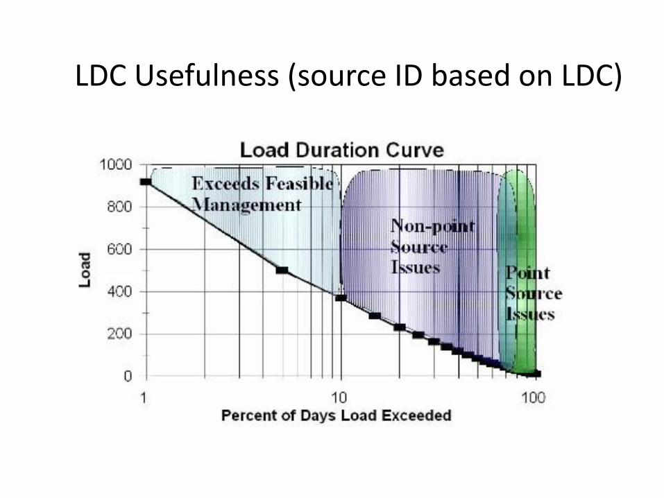
LDC Usefulness (source ID based on LDC)

• Estimate load regression curve with USGS LOAD ESTimator(LOADEST) program
• Input matching flow and E. coli concentration data• Apply regression models and choose which fits best
– 1: a0 + a1lnQ (typically best for limited flow data)– 2: a0 +a1lnQ +a2lnQ2 (typically best for more flow data)
• Have modified version of LOADEST that has E. coli constituent variables
• Calculate load regression curve from output variables and observed or simulated flow with equation:– 1: EXP(a0+a1*(LNQ- “center” of lnQ))– 2: EXP(a0+a1*(LNQ- “center” of lnQ)+a2*(LNQ- “center” of
lnQ)^2)
Copyright© Biological and Agricultural Engineering Department, Texas A&M University10
Load Regression Curve: LOADEST

Calculating Percent Reduction
• Percent Reduction calculated using formula:
– ((Loadest – TMDL) /Loadest) *100
• Percent reduction is calculated for each point and then points within a flow condition are averaged together to get the percent reduction for a flow condition

Copyright© Biological and Agricultural Engineering Department, Texas A&M University12
Continuous flow nitrate LDC
1.E+03
1.E+04
1.E+05
1.E+06
1.E+07
1.E+08
1.E+09
0 10 20 30 40 50 60 70 80 90 100
Nit
rate
Lo
ad (
g/d
ay)
Percent of Load Exceeded
Haberle Rd Load Duration Curve
Maximum Allowable Nitrate Load with 10% MOS
Load Regression Curve
Mid-Range
Low Flows

Copyright© Biological and Agricultural Engineering Department, Texas A&M University13
Developed Flow Conditions: Percent Reductions
Flow Conditions Percent Reduction Flow Percentage
High Flows 82 0-10%
Mid-Range 83 10%-75%
Low Flows 85 75%-100%

Copyright© Biological and Agricultural Engineering Department, Texas A&M University14
Flow grab sample E. coli LDC
Copyright© Biological and Agricultural Engineering Department, Texas A&M University15
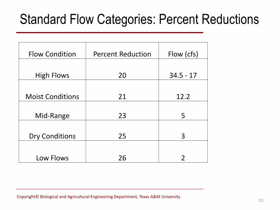
Standard Flow Categories: Percent Reductions
Flow Condition Percent Reduction Flow (cfs)
High Flows 20 34.5 - 17
Moist Conditions 21 12.2
Mid-Range 23 5
Dry Conditions 25 3
Low Flows 26 2
Recommended