
INTRODUCTION TO SHAPE OPTIMIZATION
Pierre DUYSINX
LTAS – Automotive Engineering
Academic year 2017-2018
1
Introduction
– Shape description approaches
Parametric CAD description
– Parametric design
– Sensitivity analysis & velocity field problem
– Example: The torque arm problem
– Shape optimisation and FE error control
– Boss Quattro system
2
LAYOUT
XFEM AND LEVEL SET APPROACHES
– Level Set Description
– XFEM
– Sensitivity analysis
– Examples
SHAPE OPTIMIZATION OF FLEXIBLE COMPONENTS IN MULTIBODY SYSTEMS
– Shape description
– Sensitivity analysis
– Examples
TOPOLOGY AND SHAPE OPTIMIZATION
– Case study of the mass minimization of differential casing 3
LAYOUT
ALTERNATIVE PARAMETRISATIONS FOR
TOPOLOGY OPTIMIZATION
4
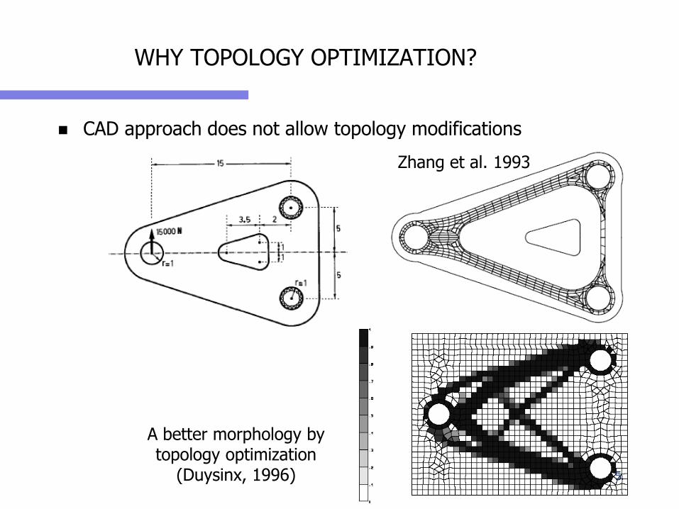
WHY TOPOLOGY OPTIMIZATION?
CAD approach does not allow topology modifications
A better morphology by topology optimization
(Duysinx, 1996)
Zhang et al. 1993
5
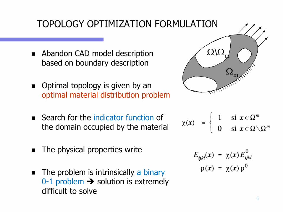
TOPOLOGY OPTIMIZATION FORMULATION
Abandon CAD model description based on boundary description
Optimal topology is given by an optimal material distribution problem
Search for the indicator function of the domain occupied by the material
The physical properties write
The problem is intrinsically a binary 0-1 problem solution is extremely
difficult to solve6
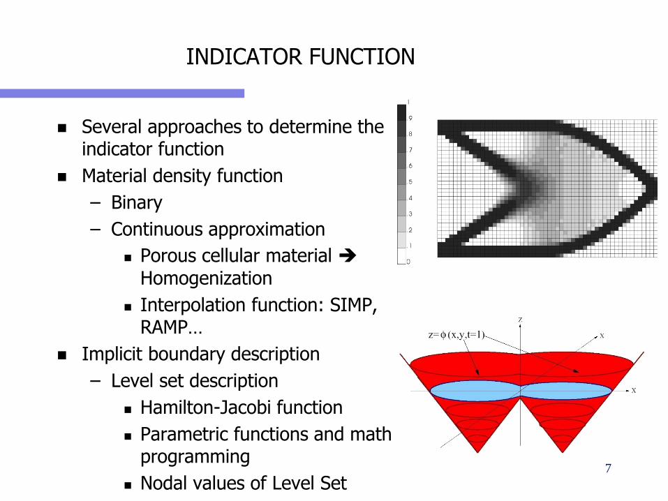
INDICATOR FUNCTION
Several approaches to determine the indicator function
Material density function
– Binary
– Continuous approximation
Porous cellular material
Homogenization
Interpolation function: SIMP, RAMP…
Implicit boundary description
– Level set description
Hamilton-Jacobi function
Parametric functions and math programming
Nodal values of Level Set
– Phase Field Description
7
SHAPE OPTIMIZATION USINGPARAMETRIC BOUNDARY DESCRIPTION
8
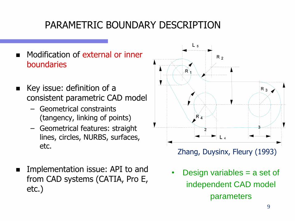
Modification of external or inner boundaries
Key issue: definition of a consistent parametric CAD model
– Geometrical constraints (tangency, linking of points)
– Geometrical features: straight lines, circles, NURBS, surfaces, etc.
Implementation issue: API to and from CAD systems (CATIA, Pro E, etc.)
PARAMETRIC BOUNDARY DESCRIPTION
Zhang, Duysinx, Fleury (1993)
• Design variables = a set of
independent CAD model
parameters9
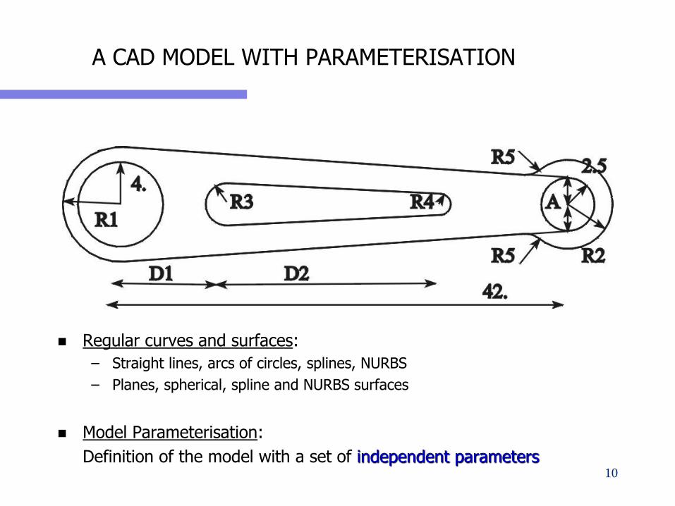
A CAD MODEL WITH PARAMETERISATION
Regular curves and surfaces:
– Straight lines, arcs of circles, splines, NURBS
– Planes, spherical, spline and NURBS surfaces
Model Parameterisation:
Definition of the model with a set of independent parameters10
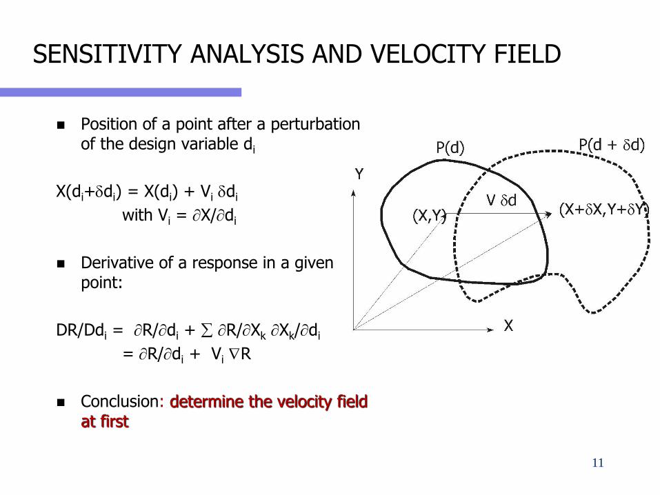
SENSITIVITY ANALYSIS AND VELOCITY FIELD
Position of a point after a perturbation of the design variable di
X(di+ddi) = X(di) + Vi ddi
with Vi = X/di
Derivative of a response in a given point:
DR/Ddi = R/di + R/Xk Xk/di
= R/di + Vi R
Conclusion: determine the velocity field at first
11
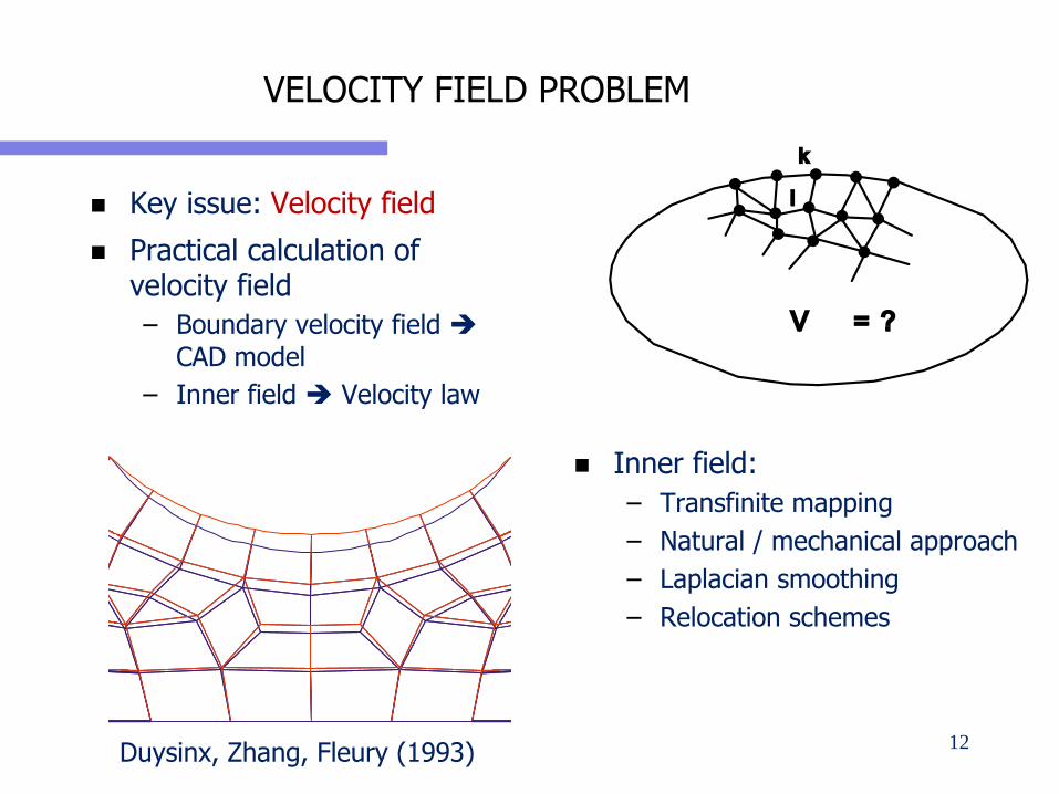
VELOCITY FIELD PROBLEM
Key issue: Velocity field
Practical calculation of velocity field
– Boundary velocity field
CAD model
– Inner field Velocity law
Inner field:
– Transfinite mapping
– Natural / mechanical approach
– Laplacian smoothing
– Relocation schemes
Duysinx, Zhang, Fleury (1993) 12
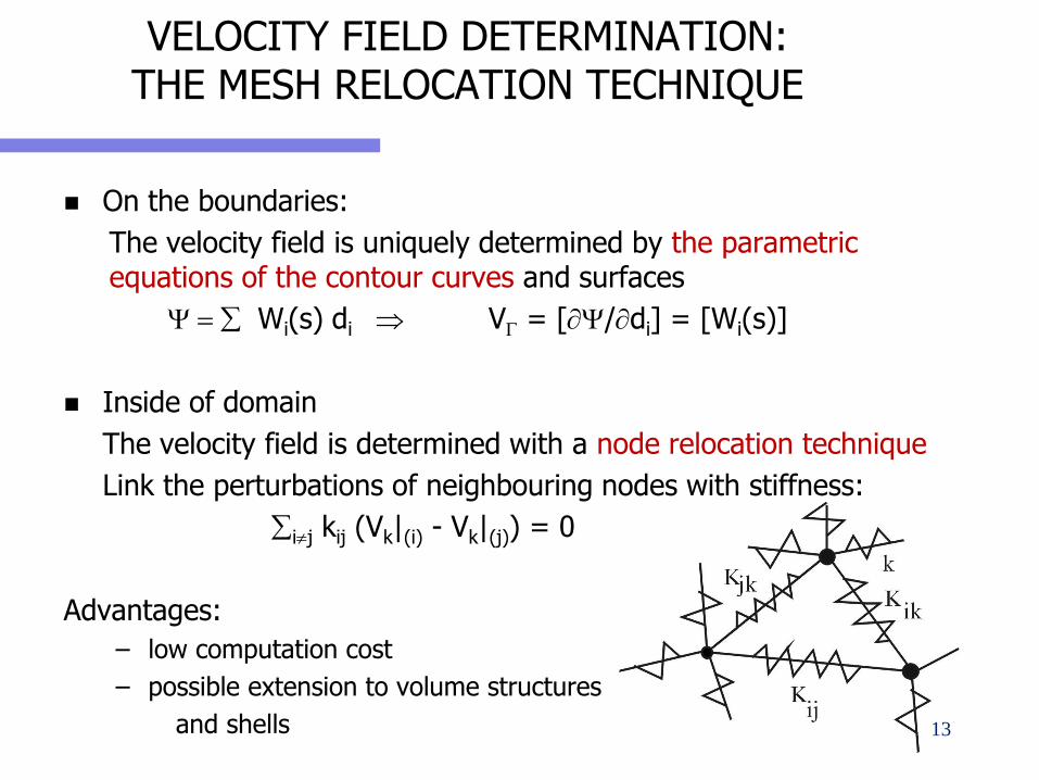
VELOCITY FIELD DETERMINATION: THE MESH RELOCATION TECHNIQUE
On the boundaries:
The velocity field is uniquely determined by the parametric equations of the contour curves and surfaces
Y = Wi(s) di VG = [Y/di] = [Wi(s)]
Inside of domain
The velocity field is determined with a node relocation technique
Link the perturbations of neighbouring nodes with stiffness:
ij kij (Vk|(i) - Vk|(j)) = 0
Advantages:
– low computation cost
– possible extension to volume structures
and shells 13
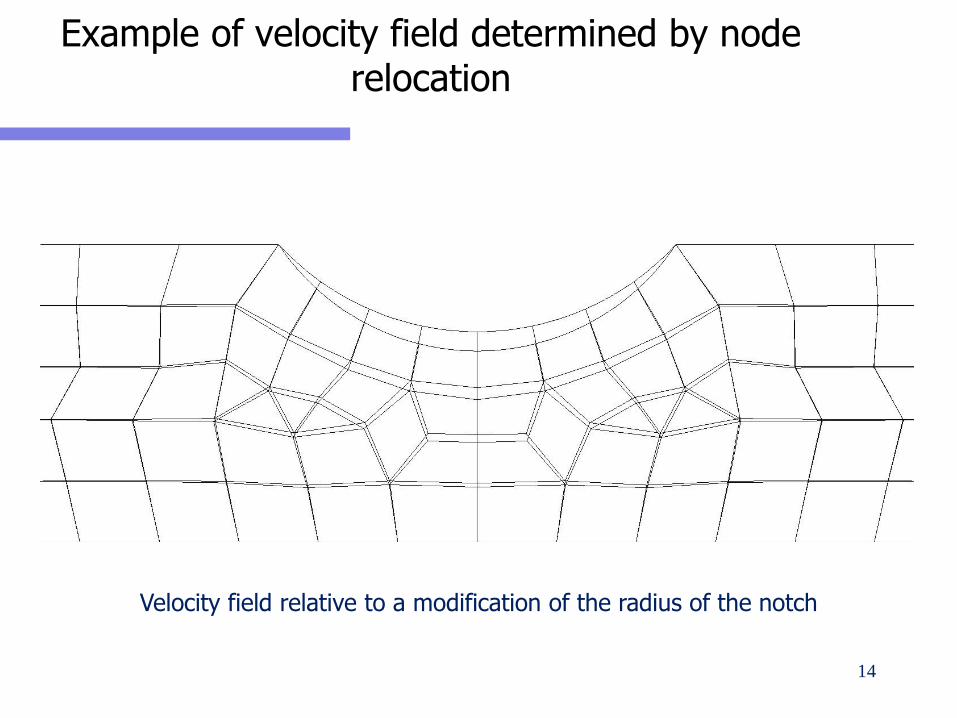
Example of velocity field determined by node relocation
Velocity field relative to a modification of the radius of the notch
14
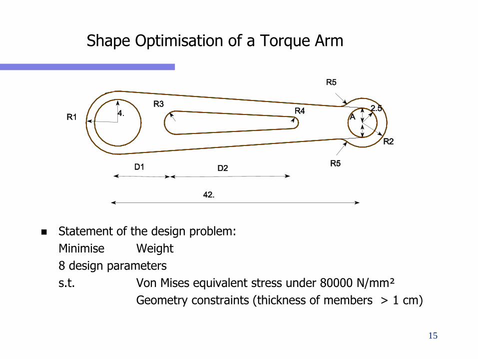
Shape Optimisation of a Torque Arm
Statement of the design problem:
Minimise Weight
8 design parameters
s.t. Von Mises equivalent stress under 80000 N/mm²
Geometry constraints (thickness of members > 1 cm)
15
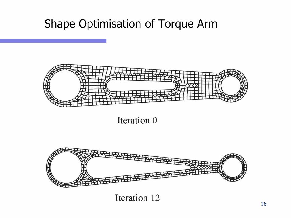
Shape Optimisation of Torque Arm
16
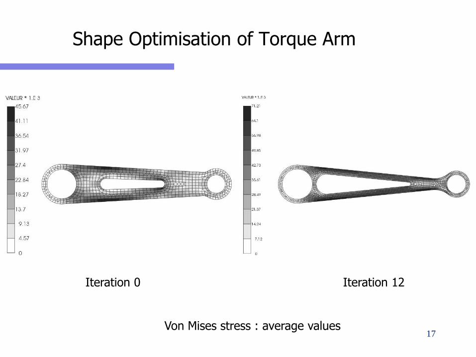
Shape Optimisation of Torque Arm
17
Iteration 0 Iteration 12
Von Mises stress : average values
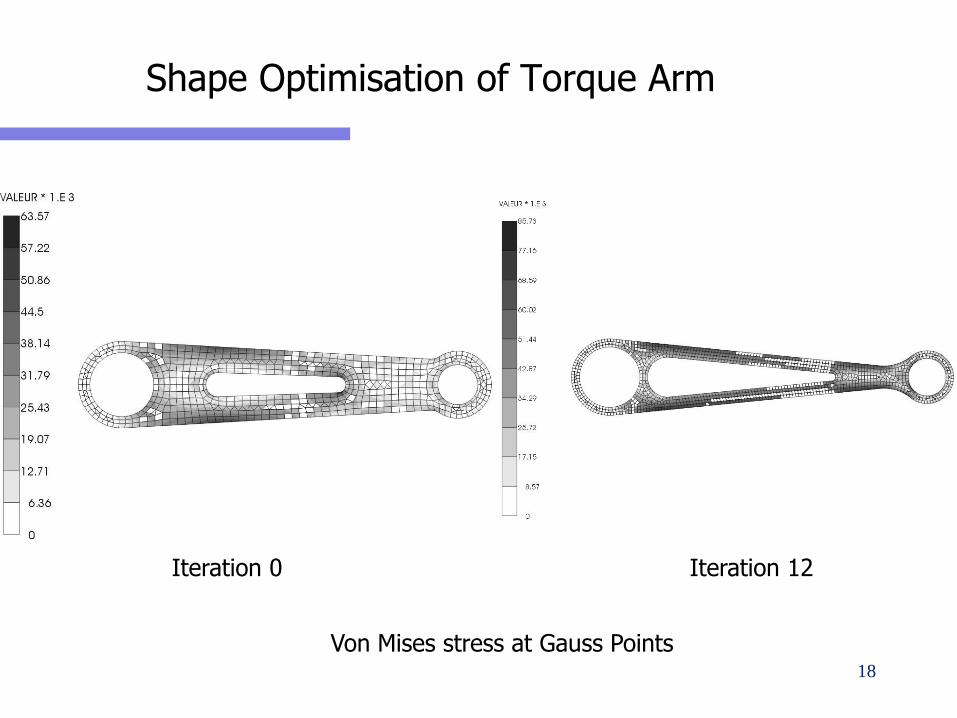
Shape Optimisation of Torque Arm
18
Iteration 0 Iteration 12
Von Mises stress at Gauss Points
SHAPE OPTIMISATION AND F.E. ERROR CONTROL
Shape modifications due to optimisation process can lead to important mesh distortions
The optimisation results are strongly dependent on the quality of the analysis (especially the stresses)
ONE ALWAYS OPTIMISES THE MODEL
To have relevant and meaningful results
CONTROL THE ERROR LEVEL OF THE ANALYSIS
Integration of an error estimation procedure and of a mesh adaptation tool into the optimisation loop
19
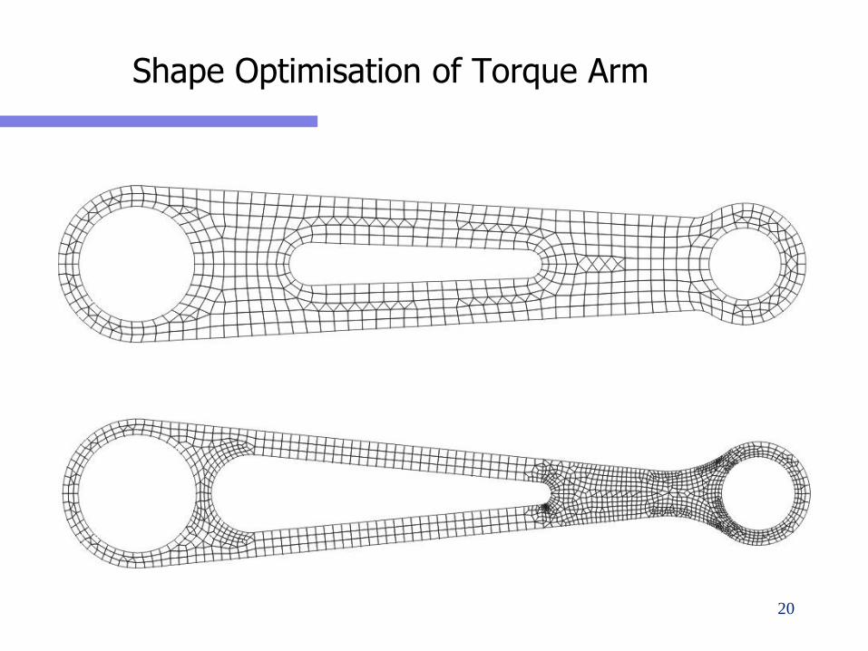
Shape Optimisation of Torque Arm
20
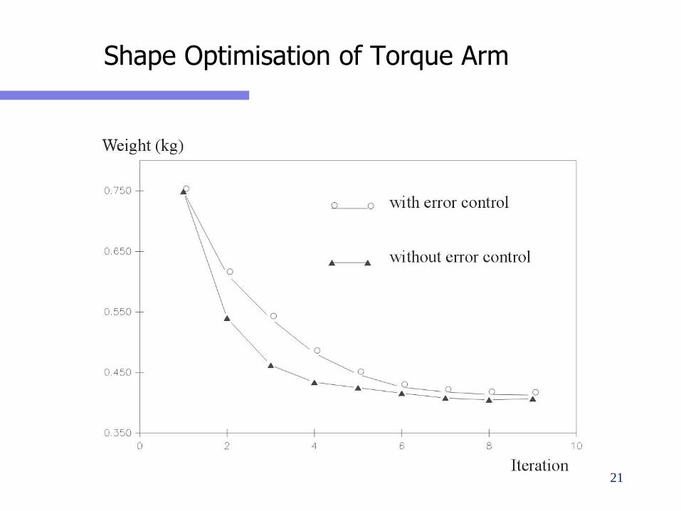
Shape Optimisation of Torque Arm
21
BOSS-Quattro
These Concepts have been implemented in a commercialised tool BOSS-Quattro developed by SAMTECH in partnership with LTAS (Ulg)
Optimisation of parametric models
Open system
A design environment for multi-model / multidisciplinary problems
Object oriented code
Optimisation algorithms
Application manager (more than a task manager)
Model manager (update, perturbations, etc.)
22
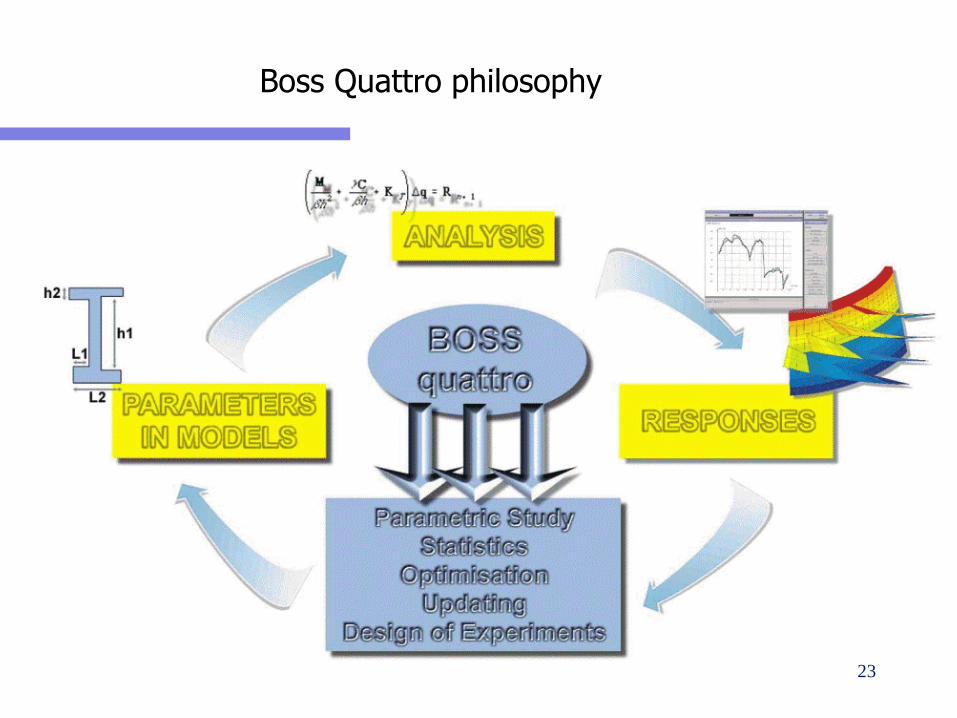
Boss Quattro philosophy
23
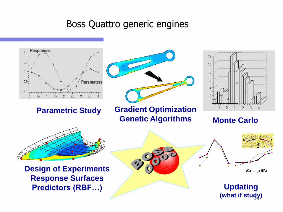
Boss Quattro generic engines
Parametric Study Gradient Optimization
Genetic Algorithms
Design of Experiments
Response Surfaces
Predictors (RBF…) Updating (what if study)
Monte Carlo
24
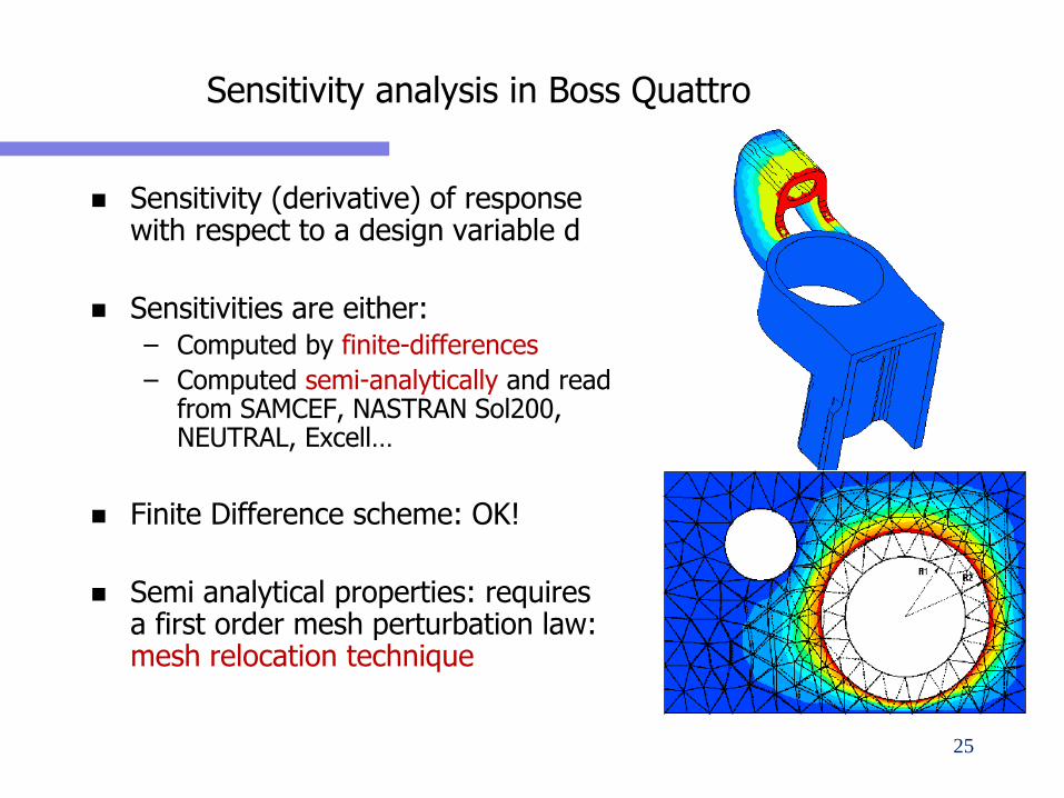
Sensitivity analysis in Boss Quattro
Sensitivity (derivative) of response with respect to a design variable d
Sensitivities are either:– Computed by finite-differences
– Computed semi-analytically and read from SAMCEF, NASTRAN Sol200, NEUTRAL, Excell…
Finite Difference scheme: OK!
Semi analytical properties: requires a first order mesh perturbation law: mesh relocation technique
25
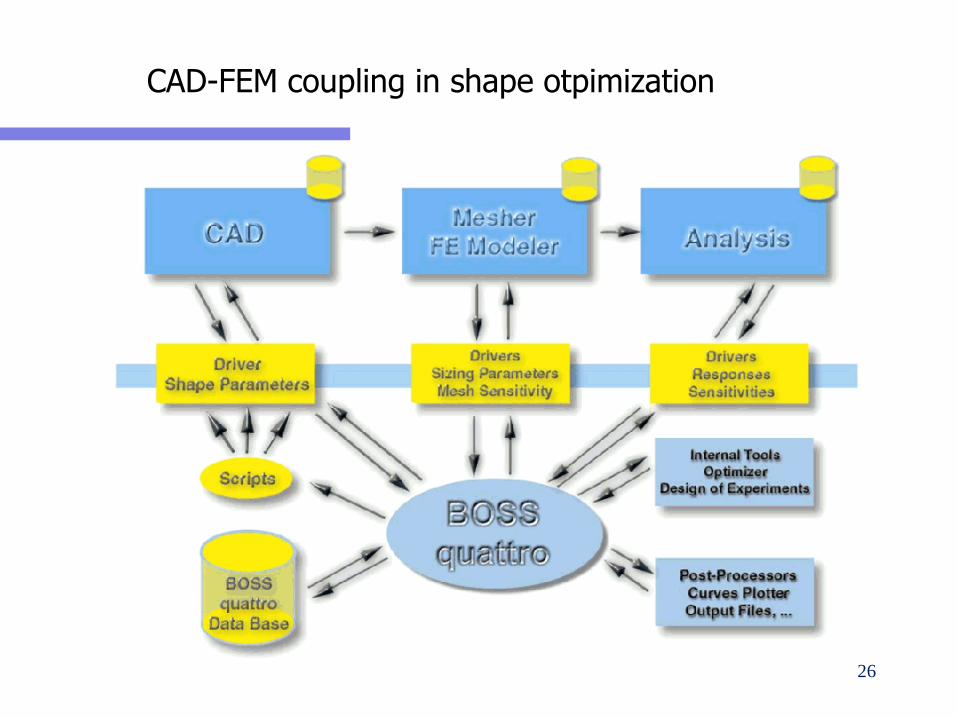
CAD-FEM coupling in shape otpimization
26
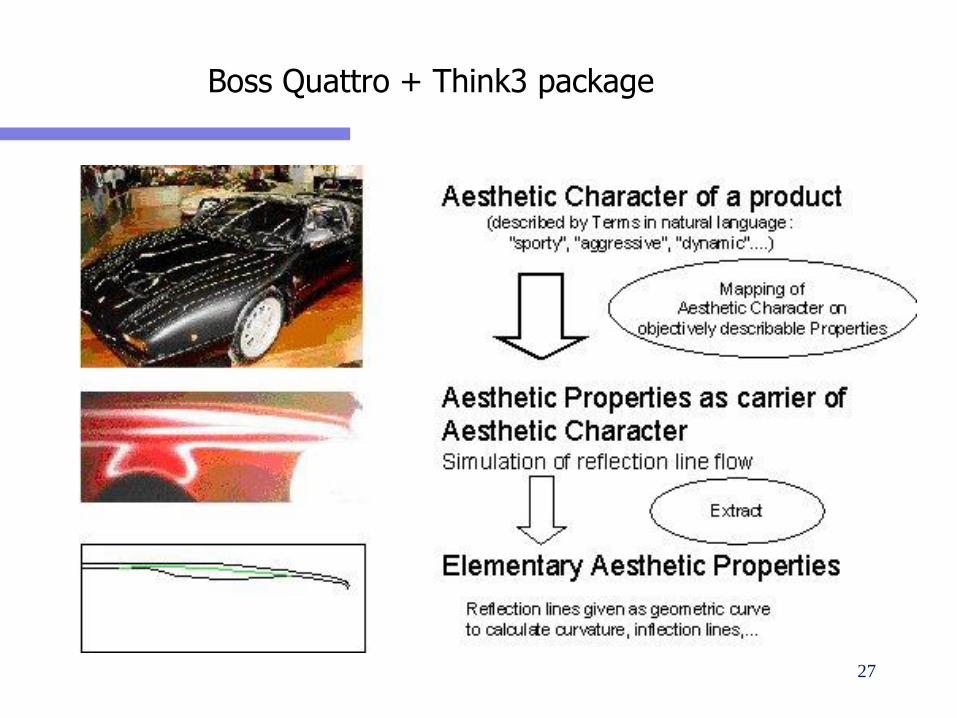
Boss Quattro + Think3 package
27
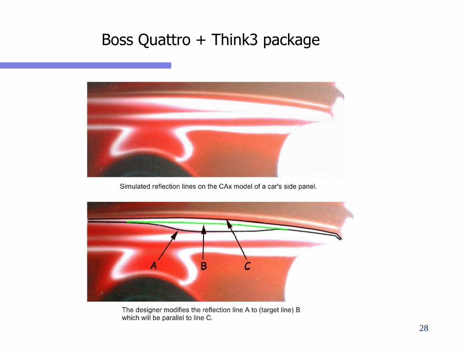
Boss Quattro + Think3 package
28
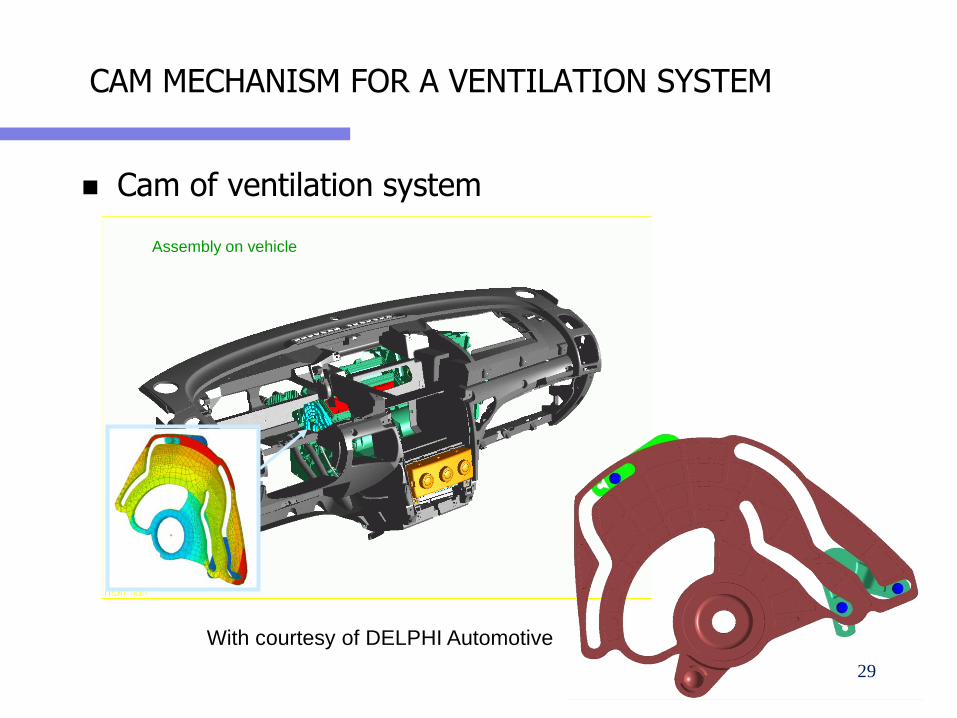
CAM MECHANISM FOR A VENTILATION SYSTEM
Cam of ventilation system
Assembly on vehicle
With courtesy of DELPHI Automotive
29
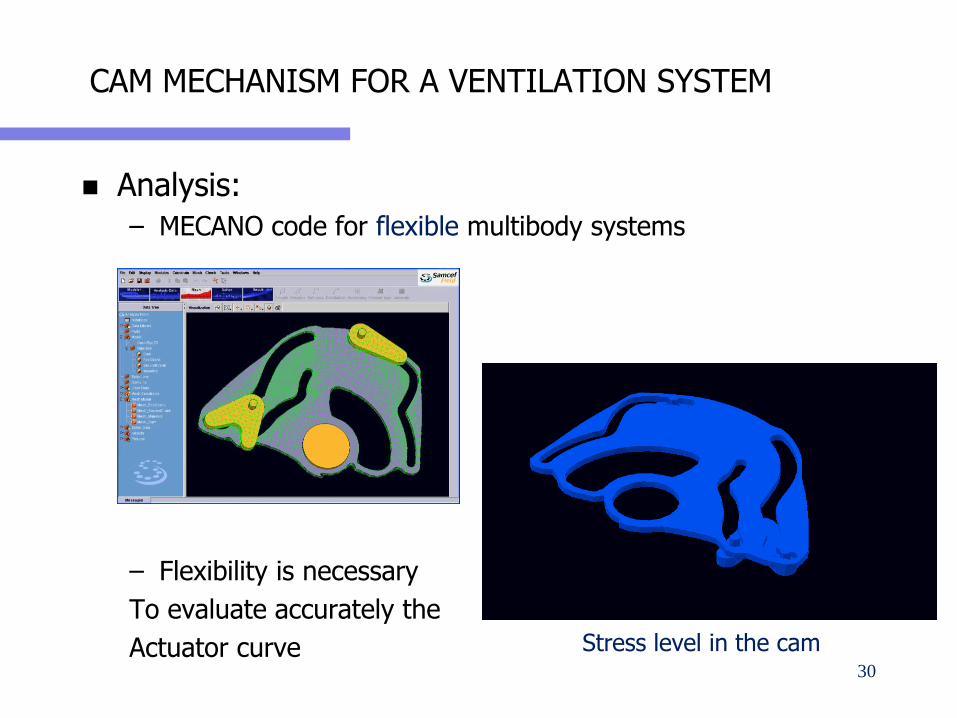
CAM MECHANISM FOR A VENTILATION SYSTEM
Analysis:
– MECANO code for flexible multibody systems
– Flexibility is necessary
To evaluate accurately the
Actuator curve Stress level in the cam30
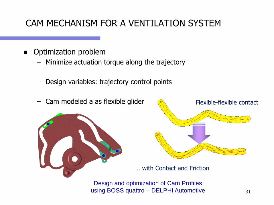
CAM MECHANISM FOR A VENTILATION SYSTEM
Optimization problem
– Minimize actuation torque along the trajectory
– Design variables: trajectory control points
– Cam modeled a as flexible glider
Design and optimization of Cam Profiles
using BOSS quattro – DELPHI Automotive
Flexible-flexible contact
… with Contact and Friction
31
XFEM and LEVEL SET OPTIMIZATION
32
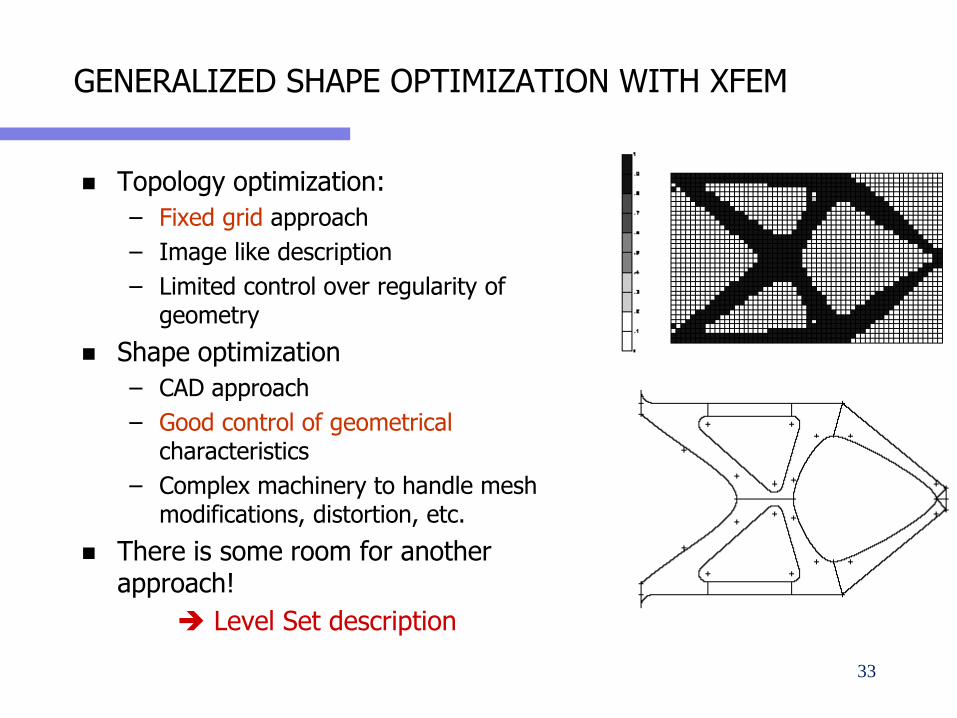
GENERALIZED SHAPE OPTIMIZATION WITH XFEM
Topology optimization:
– Fixed grid approach
– Image like description
– Limited control over regularity of geometry
Shape optimization
– CAD approach
– Good control of geometricalcharacteristics
– Complex machinery to handle mesh modifications, distortion, etc.
There is some room for another approach!
Level Set description
33
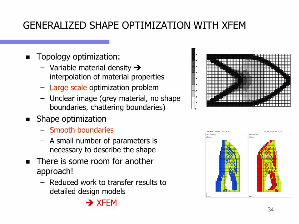
GENERALIZED SHAPE OPTIMIZATION WITH XFEM
Topology optimization:
– Variable material density
interpolation of material properties
– Large scale optimization problem
– Unclear image (grey material, no shape boundaries, chattering boundaries)
Shape optimization
– Smooth boundaries
– A small number of parameters is necessary to describe the shape
There is some room for another approach!
– Reduced work to transfer results to detailed design models
XFEM34
GENERALIZED SHAPE OPTIMIZATION WITH XFEM
LEVEL SET METHOD
– Alternative description to parametric description of curves
– Constructive geometry using parametric level sets
EXTENDED FINITE ELEMENT METHOD (XFEM)
– Alternative to remeshing methods
– Alternative to homogenization: void is void!
XFEM + LEVEL SET METHODS
– Efficient treatment of problem involving discontinuities and propagations
– Early applications in structural optimisation Belytschko et al. (2003), Wang et al. (2003), Allaire et al. (2004)
– Problem formulation:
Global and local constraints
Limited number of design variables
35
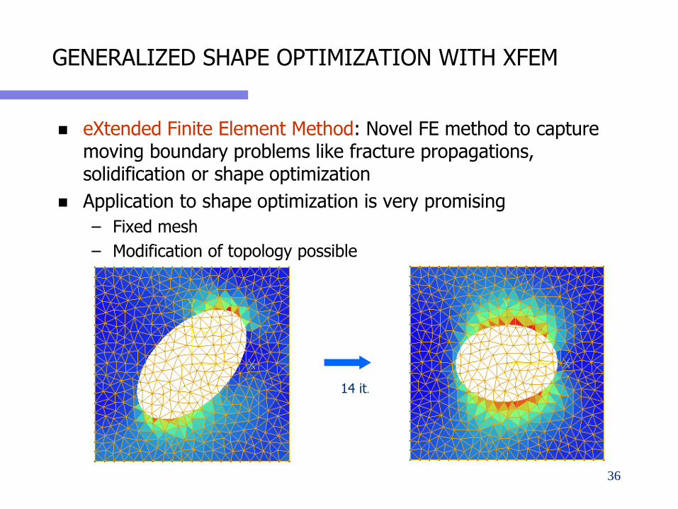
GENERALIZED SHAPE OPTIMIZATION WITH XFEM
eXtended Finite Element Method: Novel FE method to capture moving boundary problems like fracture propagations, solidification or shape optimization
Application to shape optimization is very promising
– Fixed mesh
– Modification of topology possible
14 it.
36
EXTENDED FINITE ELEMENT METHOD
Early motivation :
Study of propagating crack in mechanical structures avoid
the remeshing procedure (Moës et al IJNME Vol 46).
– Allow discontinuities inside the element
non conforming the mesh
Principle :
Allow the model to handle discontinuities that are non conforming with the mesh
Introduce additional shape functions :
To model a discontinuous behavior inside the element
To model a non polynomial response (Enrich the shape functions
space)
– Applications : cracks, holes, multi-material, multi-phases, …
37
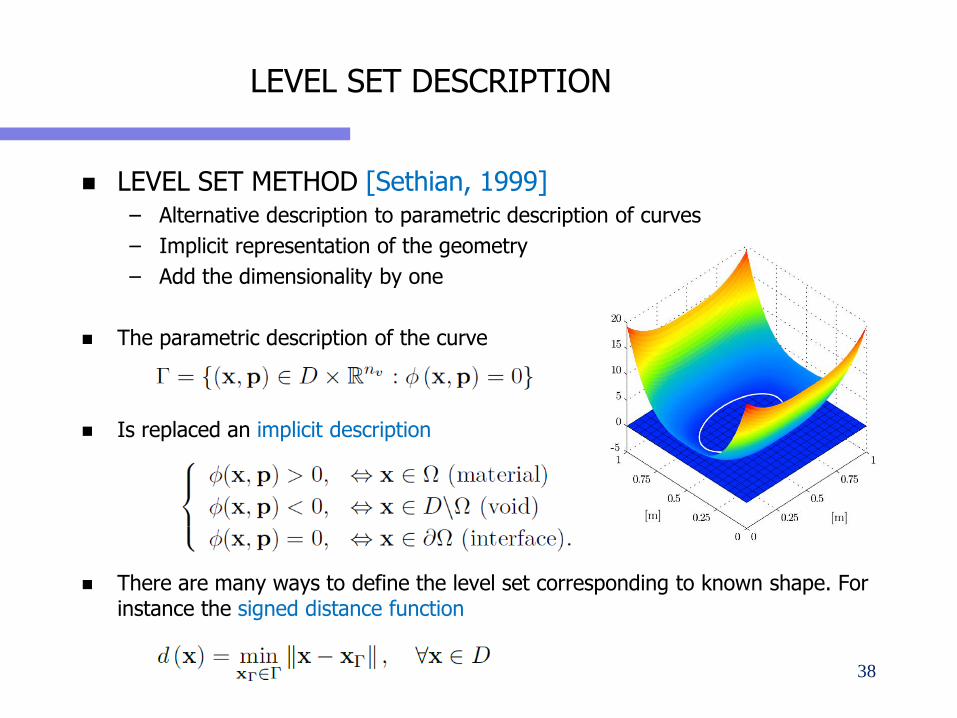
LEVEL SET DESCRIPTION
LEVEL SET METHOD [Sethian, 1999]– Alternative description to parametric description of curves
– Implicit representation of the geometry
– Add the dimensionality by one
The parametric description of the curve
Is replaced an implicit description
There are many ways to define the level set corresponding to known shape. For instance the signed distance function
38
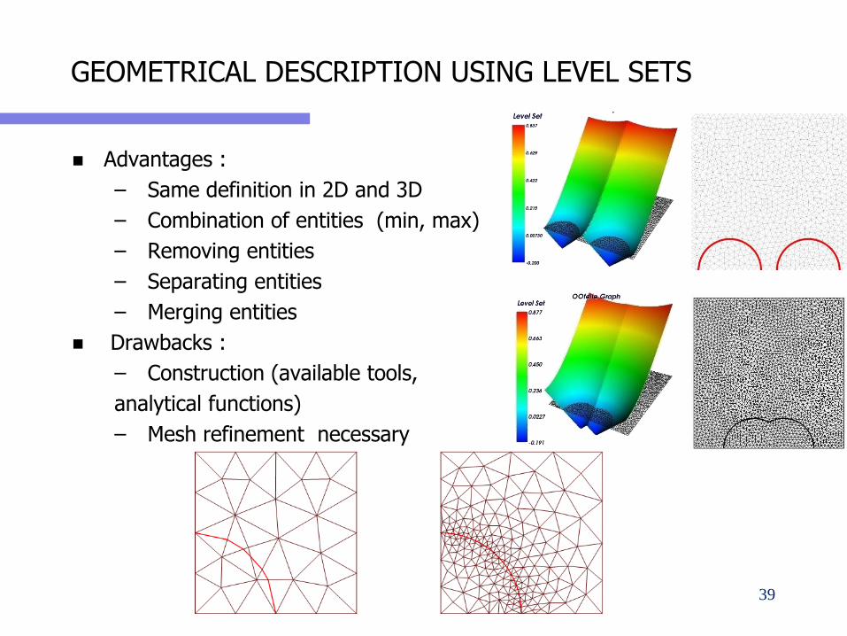
GEOMETRICAL DESCRIPTION USING LEVEL SETS
Advantages :
– Same definition in 2D and 3D
– Combination of entities (min, max)
– Removing entities
– Separating entities
– Merging entities
Drawbacks :
– Construction (available tools,
analytical functions)
– Mesh refinement necessary
39
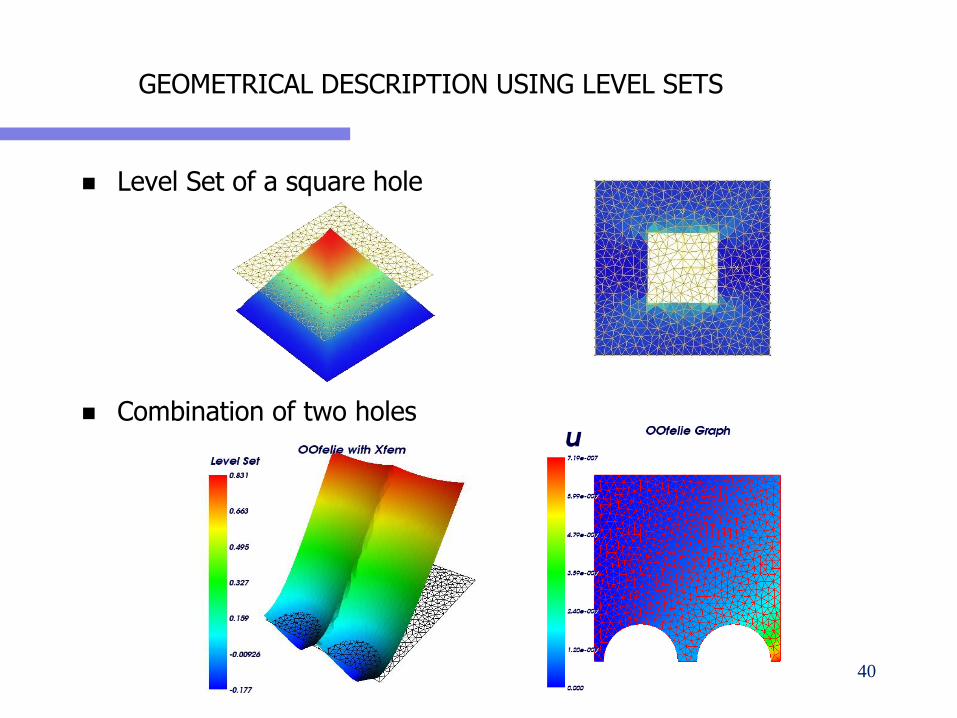
GEOMETRICAL DESCRIPTION USING LEVEL SETS
Level Set of a square hole
Combination of two holes
40
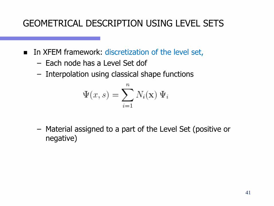
GEOMETRICAL DESCRIPTION USING LEVEL SETS
In XFEM framework: discretization of the level set,
– Each node has a Level Set dof
– Interpolation using classical shape functions
– Material assigned to a part of the Level Set (positive or negative)
41
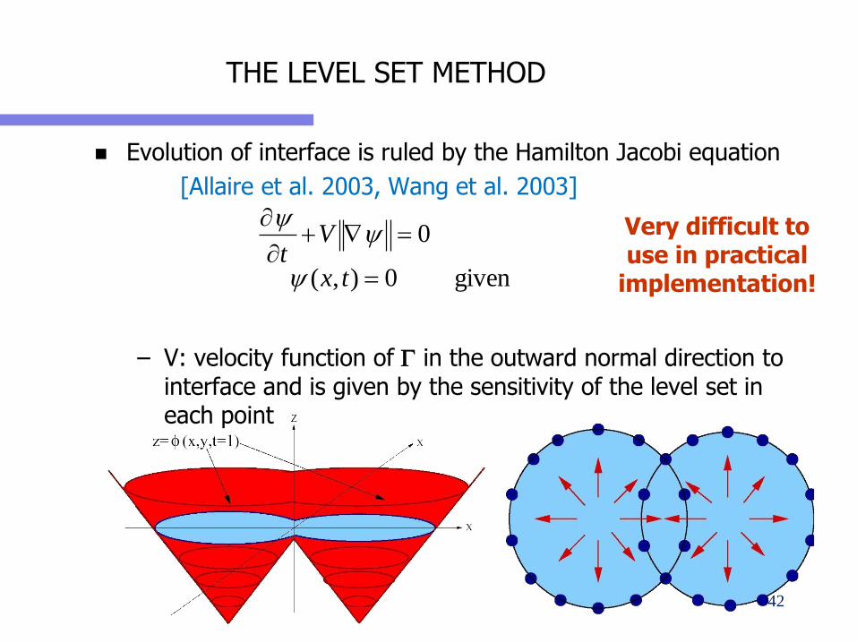
THE LEVEL SET METHOD
Evolution of interface is ruled by the Hamilton Jacobi equation
[Allaire et al. 2003, Wang et al. 2003]
– V: velocity function of G in the outward normal direction to interface and is given by the sensitivity of the level set in each point
given0),(
0
=
=
tx
Vt
Very difficult to
use in practical implementation!
42
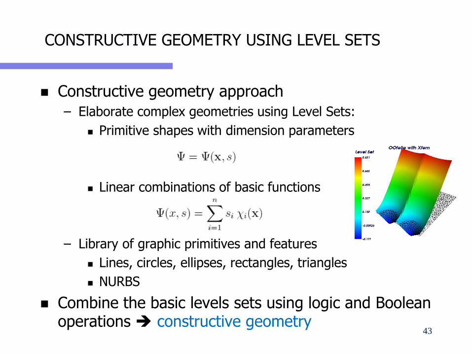
CONSTRUCTIVE GEOMETRY USING LEVEL SETS
Constructive geometry approach
– Elaborate complex geometries using Level Sets:
Primitive shapes with dimension parameters
Linear combinations of basic functions
– Library of graphic primitives and features
Lines, circles, ellipses, rectangles, triangles
NURBS
Combine the basic levels sets using logic and Boolean operations constructive geometry
43
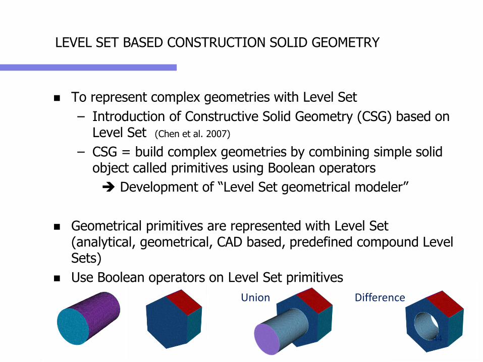
LEVEL SET BASED CONSTRUCTION SOLID GEOMETRY
To represent complex geometries with Level Set
– Introduction of Constructive Solid Geometry (CSG) based on Level Set (Chen et al. 2007)
– CSG = build complex geometries by combining simple solid object called primitives using Boolean operators
Development of “Level Set geometrical modeler”
Geometrical primitives are represented with Level Set (analytical, geometrical, CAD based, predefined compound Level Sets)
Use Boolean operators on Level Set primitives
DifferenceUnion
44
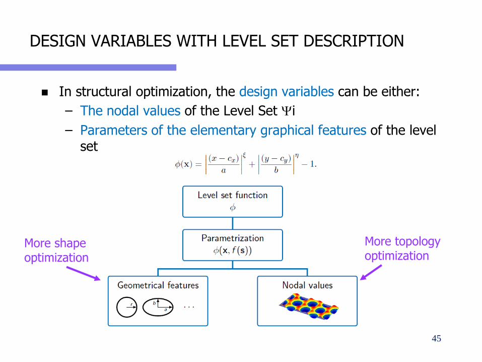
DESIGN VARIABLES WITH LEVEL SET DESCRIPTION
In structural optimization, the design variables can be either:
– The nodal values of the Level Set Yi
– Parameters of the elementary graphical features of the level set
45
More topology optimization
More shape optimization
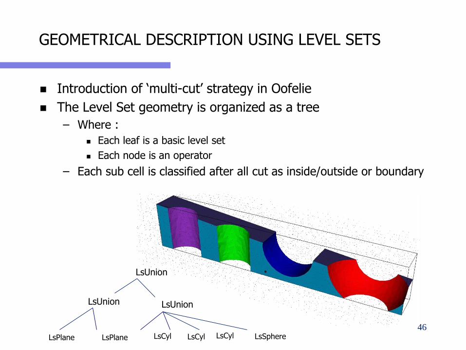
GEOMETRICAL DESCRIPTION USING LEVEL SETS
Introduction of ‘multi-cut’ strategy in Oofelie
The Level Set geometry is organized as a tree
– Where :
Each leaf is a basic level set
Each node is an operator
– Each sub cell is classified after all cut as inside/outside or boundary
LsUnion
LsUnion
LsPlane LsPlane
LsUnion
LsCyl LsCyl LsCyl LsSphere46
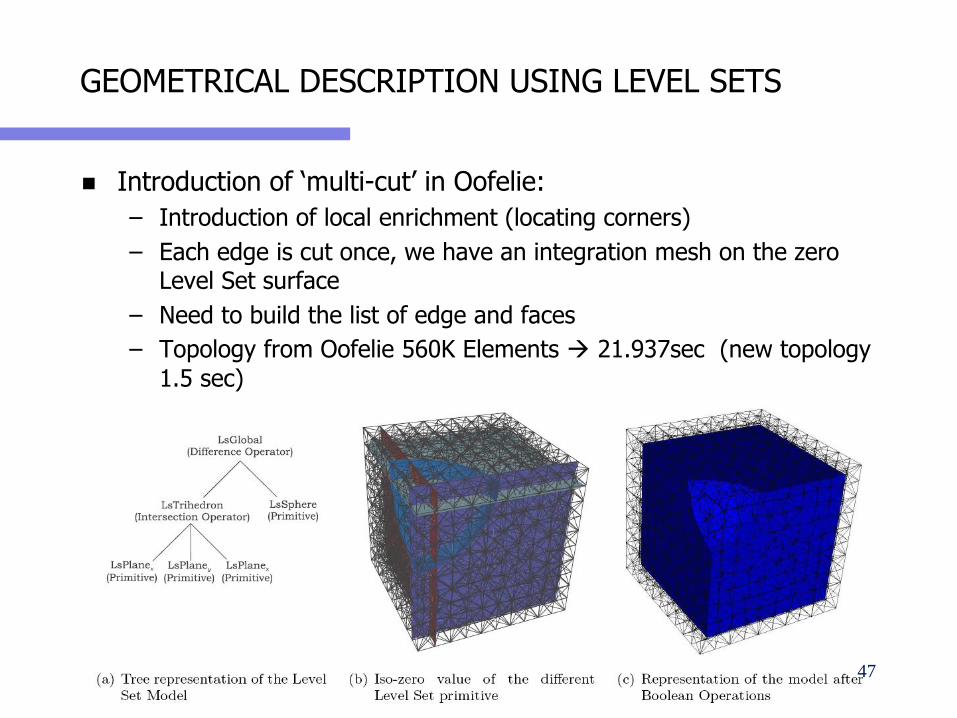
GEOMETRICAL DESCRIPTION USING LEVEL SETS
Introduction of ‘multi-cut’ in Oofelie:
– Introduction of local enrichment (locating corners)
– Each edge is cut once, we have an integration mesh on the zero Level Set surface
– Need to build the list of edge and faces
– Topology from Oofelie 560K Elements 21.937sec (new topology
1.5 sec)
(7755 Elements : FaceToFace 36.859sec)
47
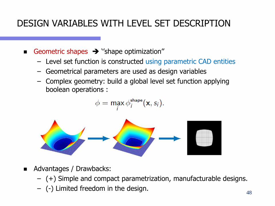
DESIGN VARIABLES WITH LEVEL SET DESCRIPTION
Geometric shapes ‘’shape optimization’’
– Level set function is constructed using parametric CAD entities
– Geometrical parameters are used as design variables
– Complex geometry: build a global level set function applying boolean operations :
Advantages / Drawbacks:
– (+) Simple and compact parametrization, manufacturable designs.
– (-) Limited freedom in the design.48
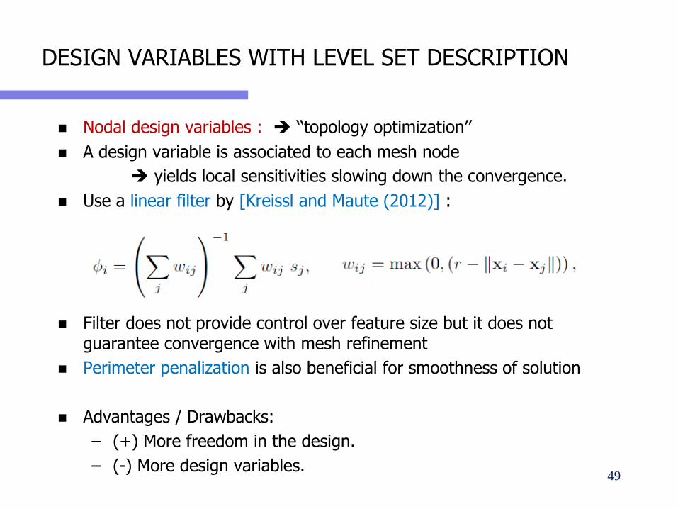
DESIGN VARIABLES WITH LEVEL SET DESCRIPTION
Nodal design variables : ‘‘topology optimization’’
A design variable is associated to each mesh node
yields local sensitivities slowing down the convergence.
Use a linear filter by [Kreissl and Maute (2012)] :
Filter does not provide control over feature size but it does not guarantee convergence with mesh refinement
Perimeter penalization is also beneficial for smoothness of solution
Advantages / Drawbacks:
– (+) More freedom in the design.
– (-) More design variables.49
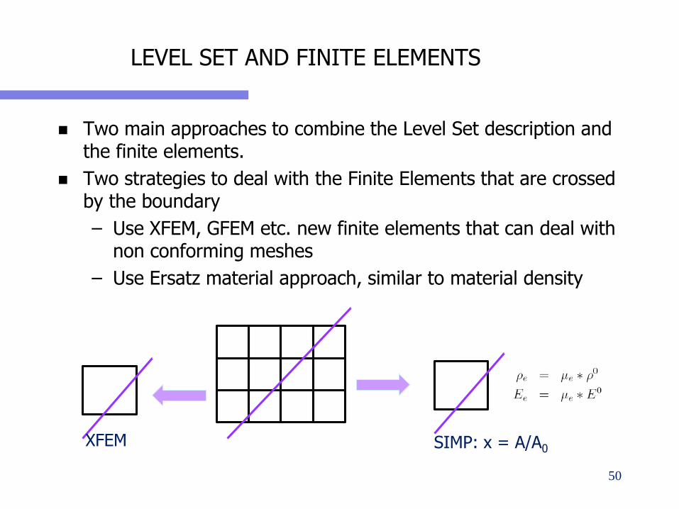
Two main approaches to combine the Level Set description and the finite elements.
Two strategies to deal with the Finite Elements that are crossed by the boundary
– Use XFEM, GFEM etc. new finite elements that can deal with non conforming meshes
– Use Ersatz material approach, similar to material density
LEVEL SET AND FINITE ELEMENTS
50
SIMP: x = A/A0XFEM
LEVEL SET DESCRIPTION AND XFEM
EXTENDED FINITE ELEMENT METHOD (XFEM)
– Early motivation : Study of propagating crack in fracture mechancs avoid the remeshing procedure (Moës et al IJNME Vol 46).
– Alternative to remeshing methods
– Alternative to homogenization: void is void!
XFEM + LEVEL SET METHODS
– Allow the model to handle evolving and propagating discontinuities that are non conforming with the mesh
– Early applications in structural optimisation Belytschko et al. (2003), Wang et al. (2003), Allaire et al. (2004)
– Problem formulation:
Access to the global and local constraints
Limited number of design variables
51
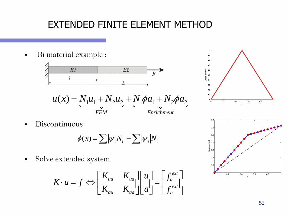
EXTENDED FINITE ELEMENT METHOD
Bi material example :
Discontinuous
Solve extended system
1 1 2 2 1 1 2 2( )
FEM Enrichment
u x N u N u N a N a =
extuu ua u
extau aa a
K K u fK u f
K K a f
= =
( ) i i i ix N N =
52
Extended Finite Element Method (XFEM)
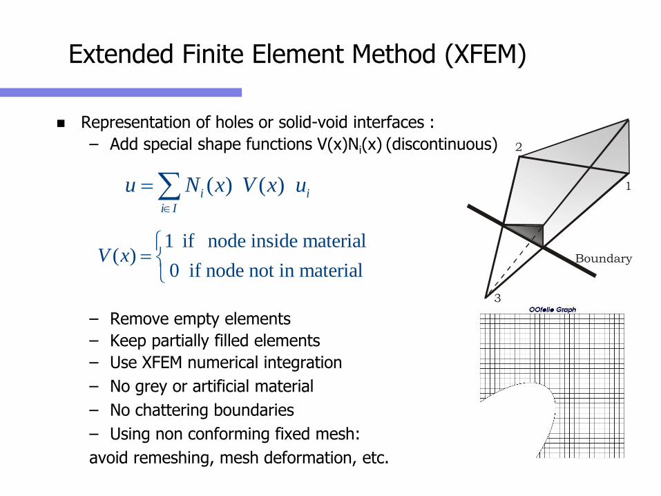
Representation of holes or solid-void interfaces :
– Add special shape functions V(x)Ni(x) (discontinuous)
– Remove empty elements
– Keep partially filled elements
– Use XFEM numerical integration
– No grey or artificial material
– No chattering boundaries
– Using non conforming fixed mesh:
avoid remeshing, mesh deformation, etc.
( ) ( )i i
i I
u N x V x u
=
1 if node inside material( )
0 if node not in materialV x
=
Boundary
3
2
1
53
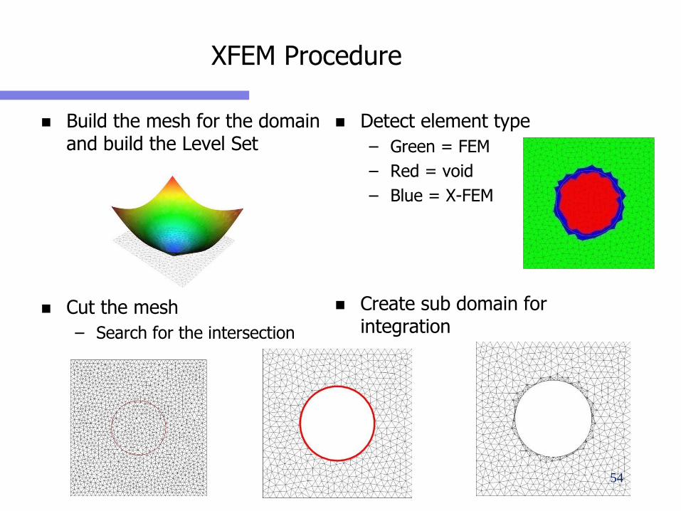
XFEM Procedure
Build the mesh for the domain and build the Level Set
Cut the mesh
– Search for the intersection
Detect element type
– Green = FEM
– Red = void
– Blue = X-FEM
Create sub domain for integration
54
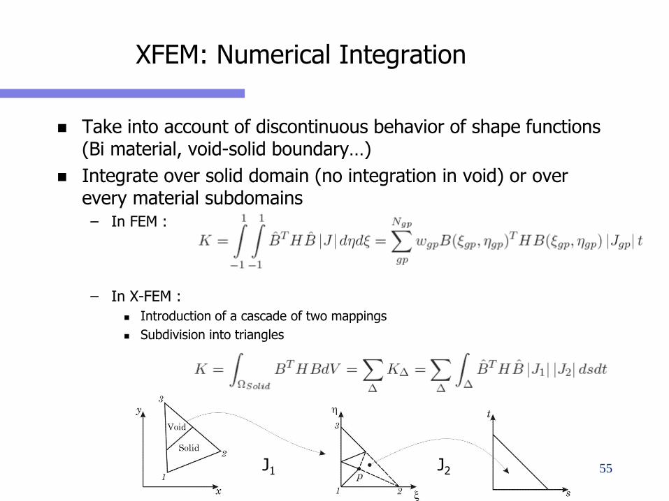
XFEM: Numerical Integration
Take into account of discontinuous behavior of shape functions (Bi material, void-solid boundary…)
Integrate over solid domain (no integration in void) or over every material subdomains– In FEM :
– In X-FEM :
Introduction of a cascade of two mappings
Subdivision into triangles
55J1 J2
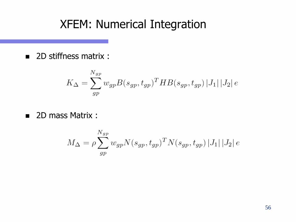
XFEM: Numerical Integration
2D stiffness matrix :
2D mass Matrix :
56
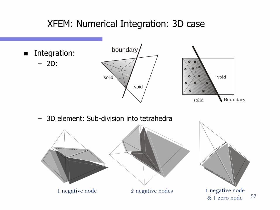
XFEM: Numerical Integration: 3D case
Integration:
– 2D:
– 3D element: Sub-division into tetrahedra
1 negative node
& 1 zero node2 negative nodes1 negative node
boundary
void
solid void
solid Boundary
57
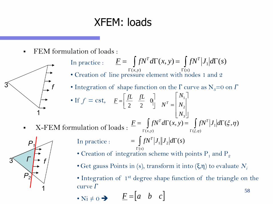
XFEM: loads
FEM formulation of loads :
X-FEM formulation of loads :
In practice :
• Creation of line pressure element with nodes 1 and 2
• Integration of shape function on the Γ curve as N3=0 on Γ
• If f = cst,
In practice :
• Creation of integration scheme with points P1 and P2
•Get gauss Points in (s), transform it into (ξ,η) to evaluate Ni
• Integration of 1st degree shape function of the triangle on the
curve Γ
• Ni ≠ 0
)(),( 1
)(),(
sdJfNyxdfNFs
T
yx
T G=G= GG
1
2
3
T
N
N N
N
=
= 0
22
fLfLF
cbaF =
)(
),(),(
21
)(
1
),(),(
sdJJfN
dJfNyxdfNF
s
T
T
yx
T
G=
G=G=
G
GG
58
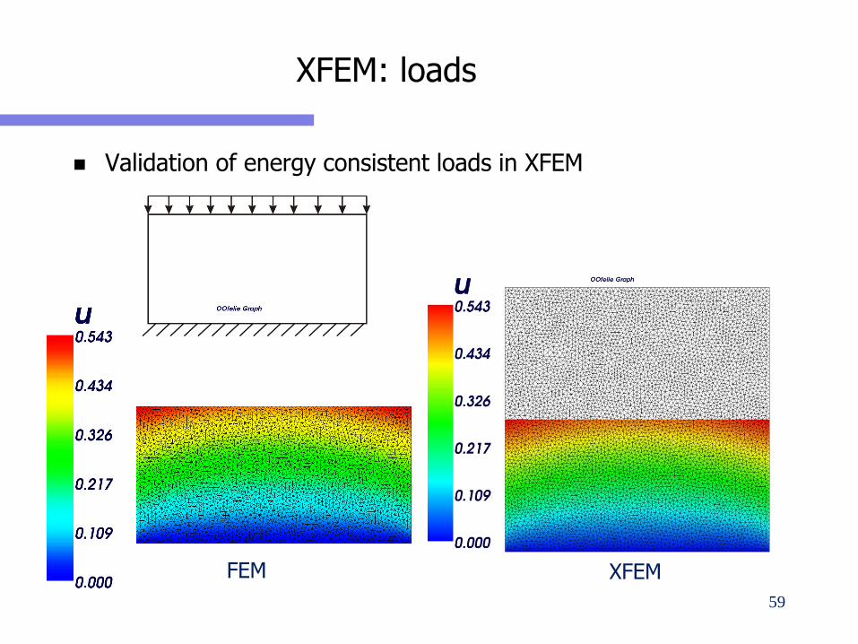
XFEM: loads
Validation of energy consistent loads in XFEM
FEM XFEM
59
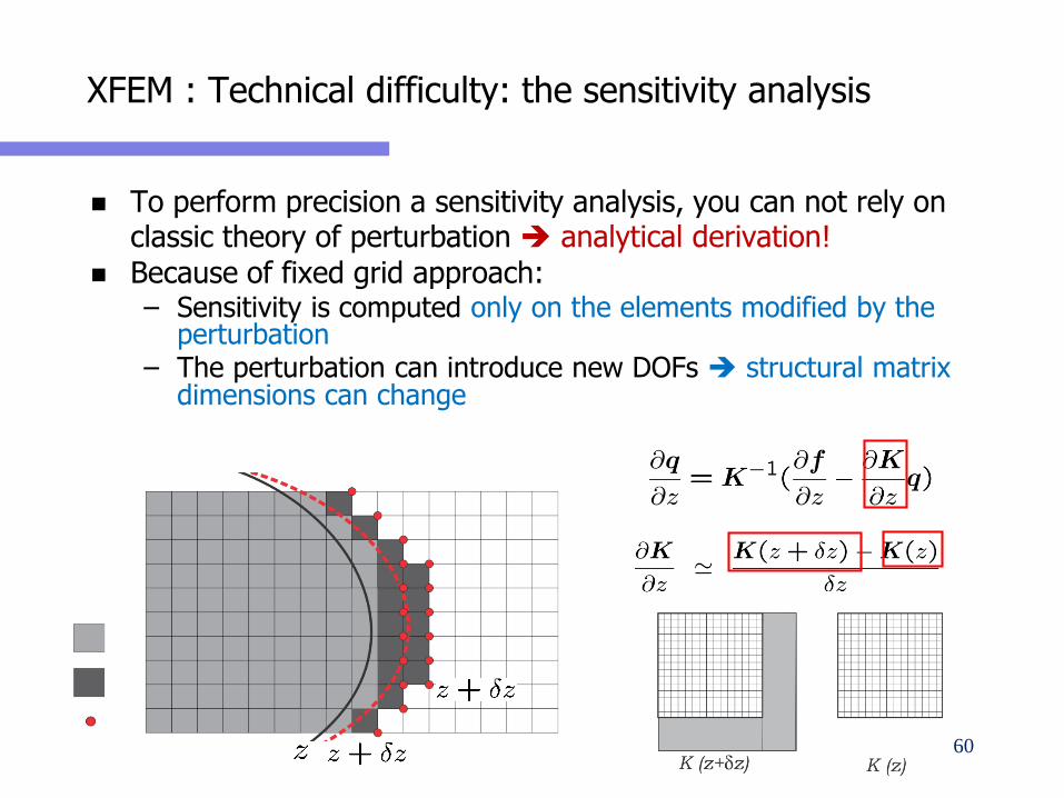
XFEM : Technical difficulty: the sensitivity analysis
To perform precision a sensitivity analysis, you can not rely on classic theory of perturbation analytical derivation!
Because of fixed grid approach:– Sensitivity is computed only on the elements modified by the
perturbation– The perturbation can introduce new DOFs structural matrix
dimensions can change
60
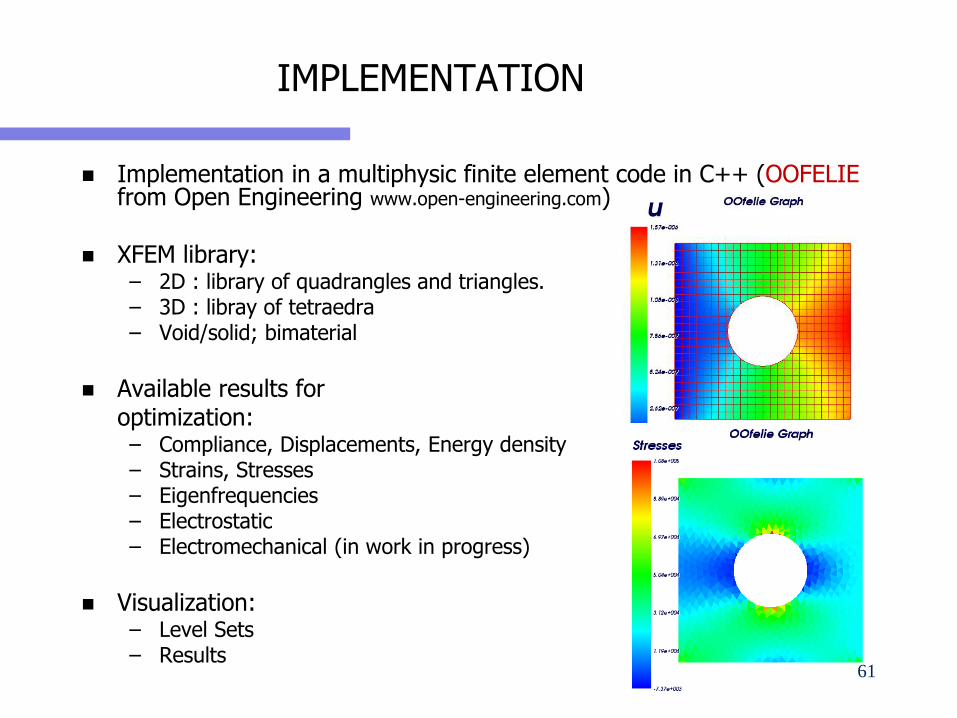
IMPLEMENTATION
Implementation in a multiphysic finite element code in C++ (OOFELIE from Open Engineering www.open-engineering.com)
XFEM library: – 2D : library of quadrangles and triangles.– 3D : libray of tetraedra– Void/solid; bimaterial
Available results for optimization:– Compliance, Displacements, Energy density– Strains, Stresses– Eigenfrequencies– Electrostatic– Electromechanical (in work in progress)
Visualization:– Level Sets– Results
61
MECHANICAL AND MANUFACTURING CONSTRAINTS
With the Level Set approach, one has access to:
– All local stress constraints with high precision
– Easier to evaluate manufacturing constraints: e.g. un molding direction, maximum size, minium size, etc. [Michailids et al. 2015]
62
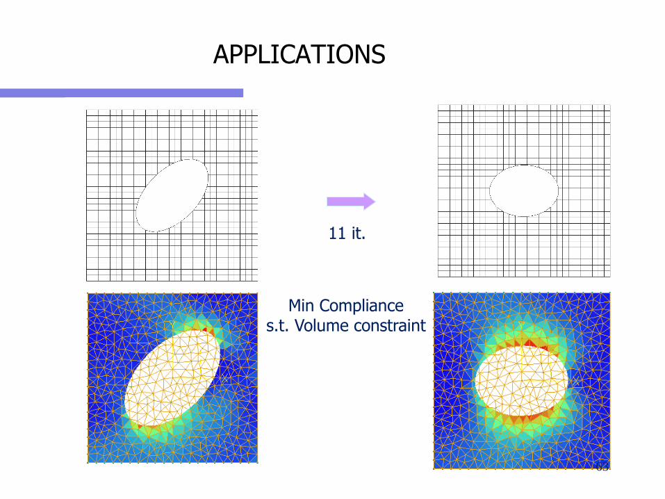
APPLICATIONS
11 it.
Min Compliances.t. Volume constraint
63
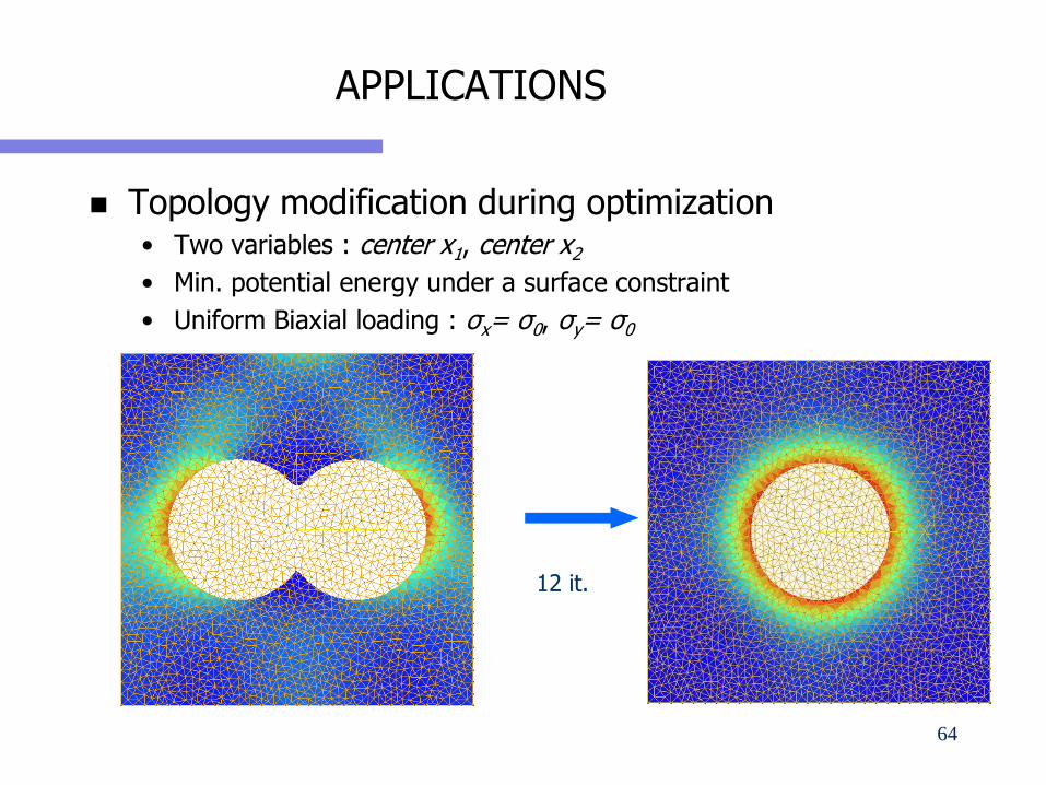
APPLICATIONS
Topology modification during optimization• Two variables : center x1, center x2
• Min. potential energy under a surface constraint
• Uniform Biaxial loading : σx= σ0, σy= σ0
12 it.
64
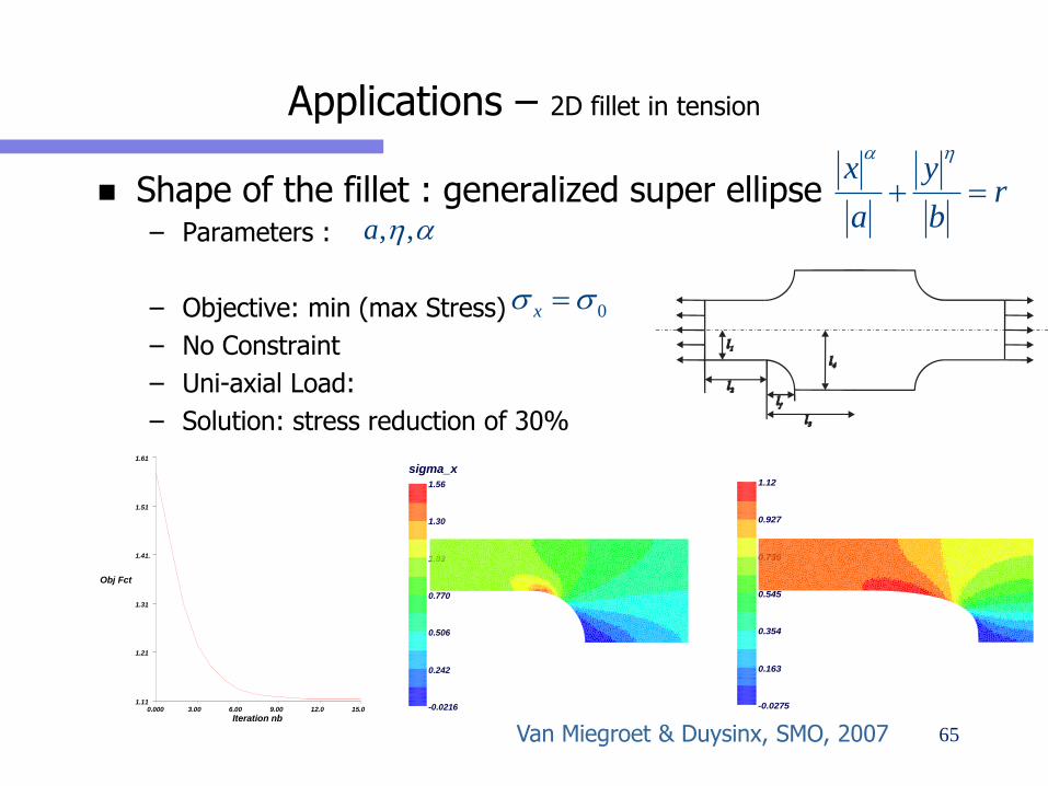
Shape of the fillet : generalized super ellipse– Parameters :
– Objective: min (max Stress)
– No Constraint
– Uni-axial Load:
– Solution: stress reduction of 30%
Applications – 2D fillet in tension
sigma_x
-0.0275-0.0275
0.163 0.163
0.354 0.354
0.545 0.545
0.736 0.736
0.927 0.927
1.12 1.12
Iteration nbIteration nb0.000 0.000 3.00 3.00 6.00 6.00 9.00 9.00 12.0 12.0 15.0 15.0
Obj FctObj Fct
1.61 1.61
1.51 1.51
1.41 1.41.
1.31 1.31
1.21. 1.21
1.11 1.11
sigma_xsigma_x
-0.0216-0.0216
0.242 0.242
0.506 0.506
0.770 0.770
1.03 1.03
1.30 1.30
1.56 1.56
x yr
a b
=
, ,a
0x =
Van Miegroet & Duysinx, SMO, 2007 65
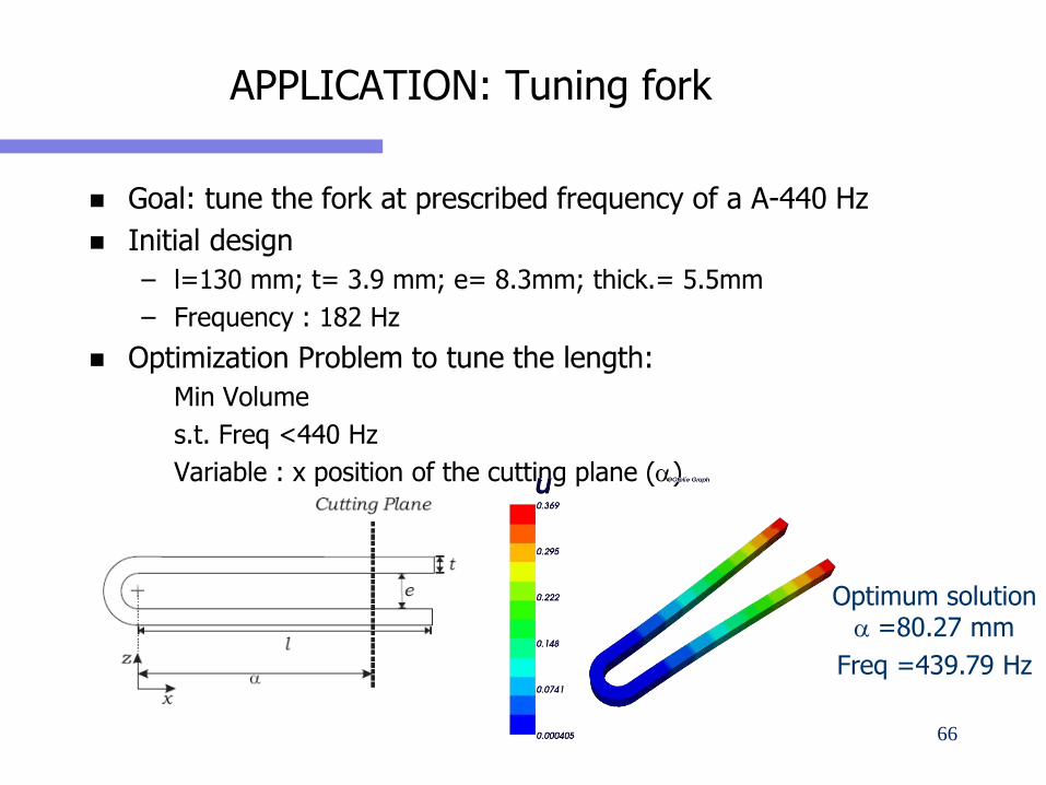
APPLICATION: Tuning fork
Goal: tune the fork at prescribed frequency of a A-440 Hz
Initial design
– l=130 mm; t= 3.9 mm; e= 8.3mm; thick.= 5.5mm
– Frequency : 182 Hz
Optimization Problem to tune the length:
Min Volume
s.t. Freq <440 Hz
Variable : x position of the cutting plane ()
Optimum solution =80.27 mm
Freq =439.79 Hz
66
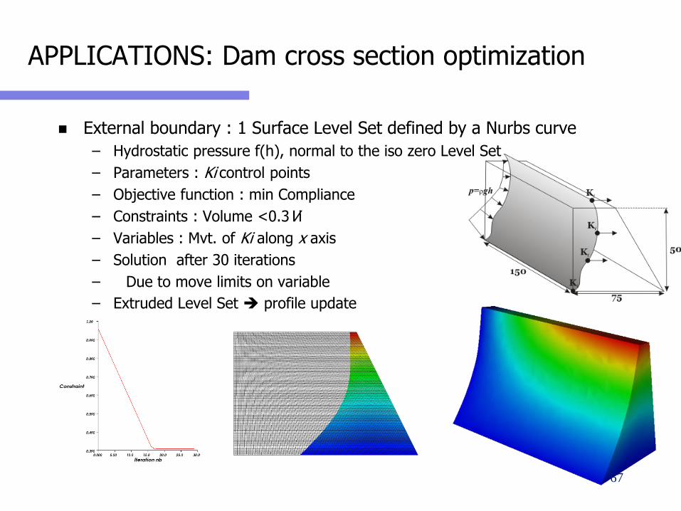
APPLICATIONS: Dam cross section optimization
External boundary : 1 Surface Level Set defined by a Nurbs curve
– Hydrostatic pressure f(h), normal to the iso zero Level Set
– Parameters : Ki control points
– Objective function : min Compliance
– Constraints : Volume <0.3Vi
– Variables : Mvt. of Ki along x axis
– Solution after 30 iterations
– Due to move limits on variable
– Extruded Level Set profile update
67
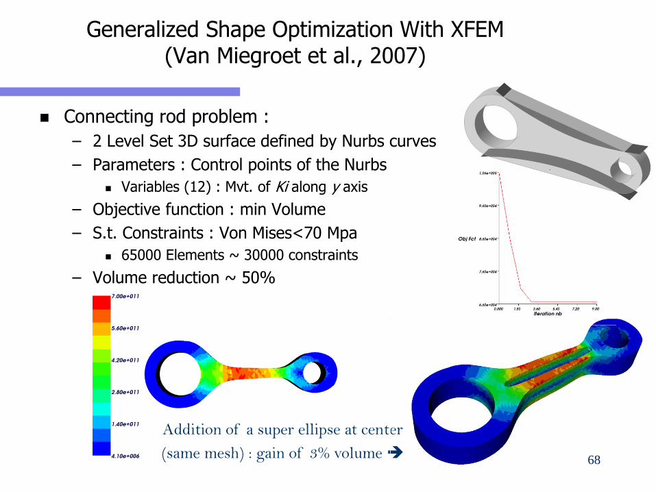
Generalized Shape Optimization With XFEM (Van Miegroet et al., 2007)
Connecting rod problem :
– 2 Level Set 3D surface defined by Nurbs curves
– Parameters : Control points of the Nurbs
Variables (12) : Mvt. of Ki along y axis
– Objective function : min Volume
– S.t. Constraints : Von Mises<70 Mpa
65000 Elements ~ 30000 constraints
– Volume reduction ~ 50%
Addition of a super ellipse at center
(same mesh) : gain of 3% volume 68
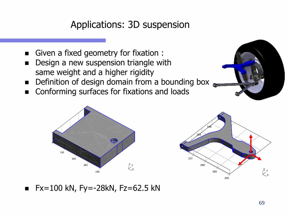
Applications: 3D suspension
Given a fixed geometry for fixation : Design a new suspension triangle with
same weight and a higher rigidity Definition of design domain from a bounding box Conforming surfaces for fixations and loads
Fx=100 kN, Fy=-28kN, Fz=62.5 kN
69
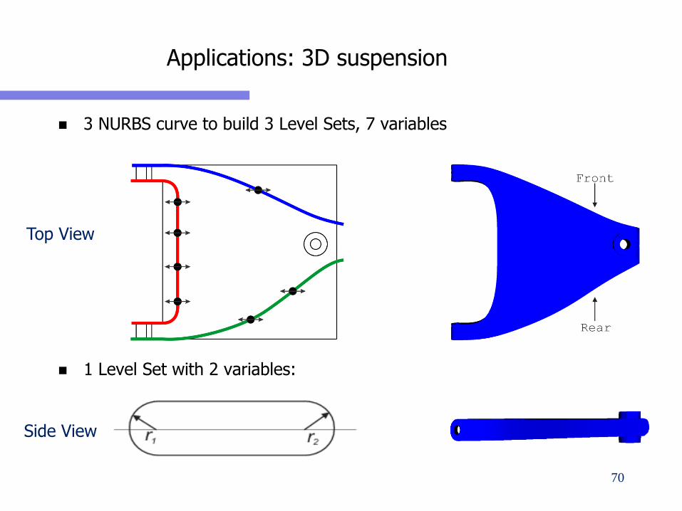
Applications: 3D suspension
3 NURBS curve to build 3 Level Sets, 7 variables
1 Level Set with 2 variables:
Top View
Side View
70
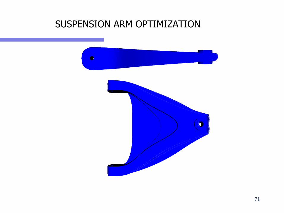
SUSPENSION ARM OPTIMIZATION
71
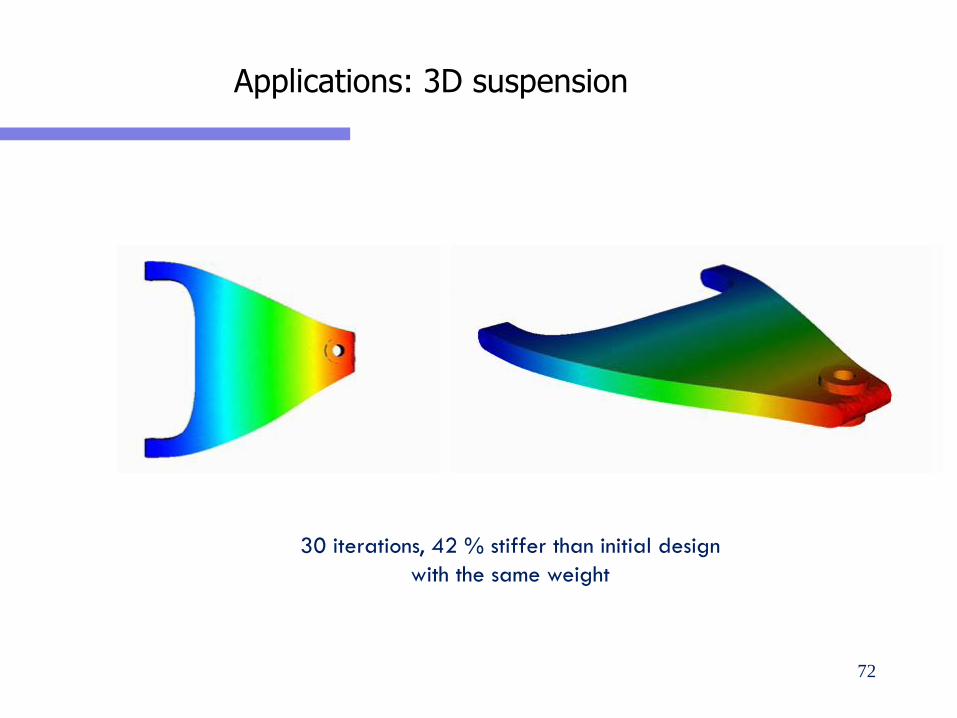
Applications: 3D suspension
30 iterations, 42 % stiffer than initial design
with the same weight
72
OPTIMIZATION OF STRUCTURAL COMPONENTS IN MULTIBODY
SYSTEMS DYNAMICS
73
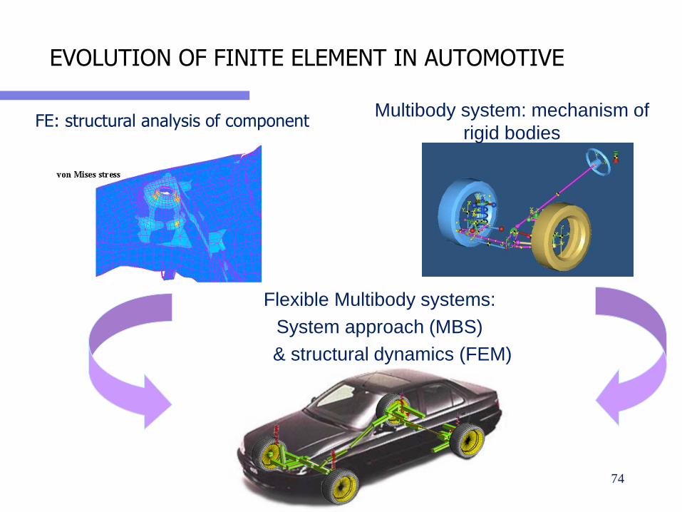
EVOLUTION OF FINITE ELEMENT IN AUTOMOTIVE
Multibody system: mechanism of
rigid bodies
Flexible Multibody systems:
System approach (MBS)
& structural dynamics (FEM)
FE: structural analysis of component
74
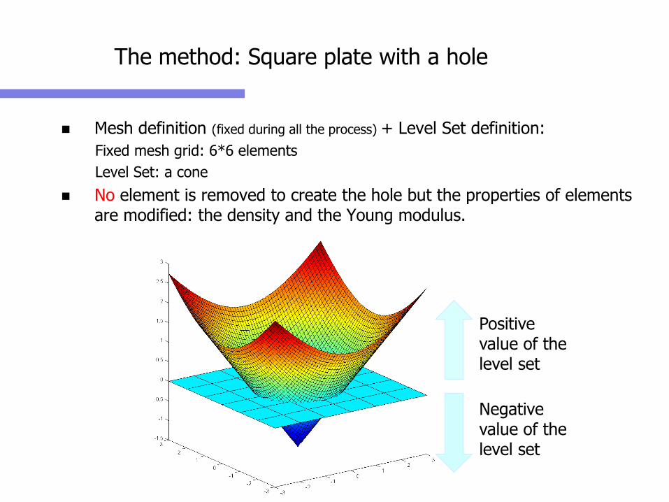
The method: Square plate with a hole
Mesh definition (fixed during all the process) + Level Set definition:
Fixed mesh grid: 6*6 elements
Level Set: a cone
No element is removed to create the hole but the properties of elements are modified: the density and the Young modulus.
Negative value of the level set
Positive value of the level set
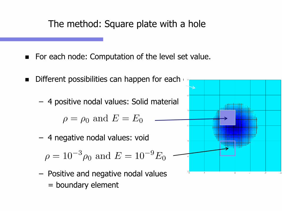
The method: Square plate with a hole
For each node: Computation of the level set value.
Different possibilities can happen for each element:
– 4 positive nodal values: Solid material
– 4 negative nodal values: void
– Positive and negative nodal values
= boundary element
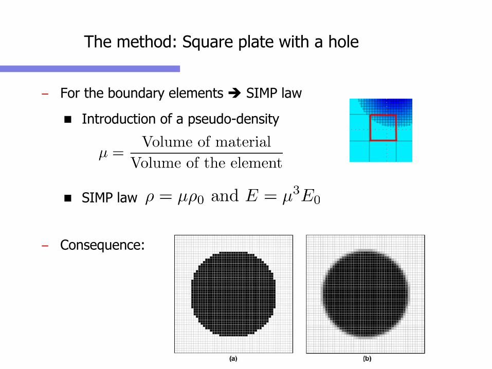
The method: Square plate with a hole
– For the boundary elements SIMP law
Introduction of a pseudo-density
SIMP law
– Consequence:
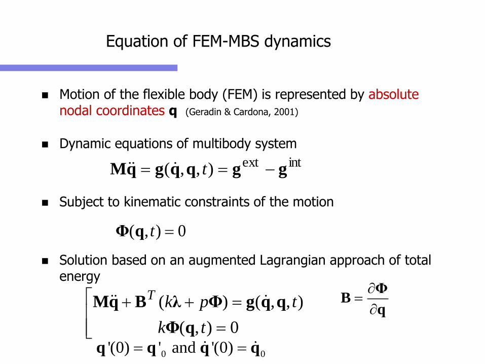
Equation of FEM-MBS dynamics
Motion of the flexible body (FEM) is represented by absolute nodal coordinates q (Geradin & Cardona, 2001)
Dynamic equations of multibody system
Subject to kinematic constraints of the motion
Solution based on an augmented Lagrangian approach of total energy
intext),,( ggqqgqM == t
0),( =tqΦ
=
=
0),(
),,()(
tk
tpkT
qΦ
qqgΦλBqM q
ΦB
=
0 0'(0) ' and '(0)= =q q q q
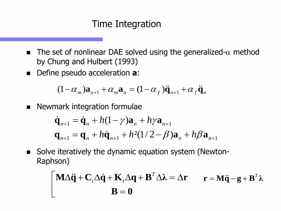
Time Integration
The set of nonlinear DAE solved using the generalized- method by Chung and Hulbert (1993)
Define pseudo acceleration a:
Newmark integration formulae
Solve iteratively the dynamic equation system (Newton-Raphson)
1 1(1 ) (1 )m n m n f n f n = a a q q
1 1(1 )n n n nh h = q q a a
1 1 1²(1/ 2 )n n n n nh h h = q q q a a
T
t t =
=
M q C q K q B λ r
B 0
T= r Mq g B λ
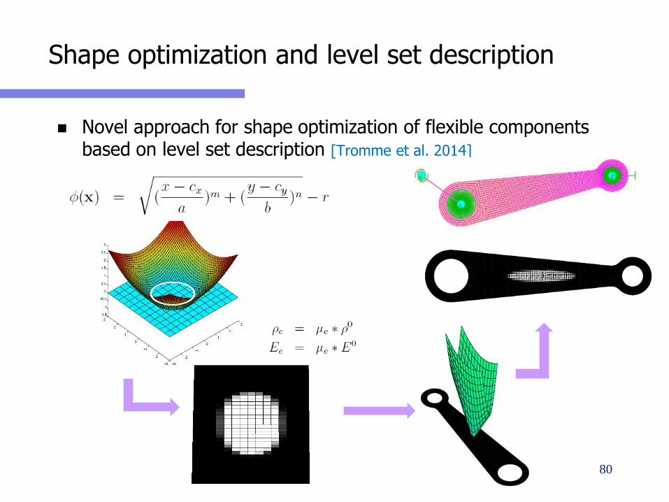
Shape optimization and level set description
Novel approach for shape optimization of flexible components based on level set description [Tromme et al. 2014]
80
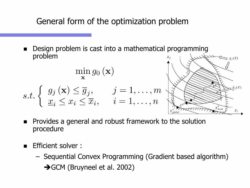
General form of the optimization problem
Design problem is cast into a mathematical programming problem
Provides a general and robust framework to the solution procedure
Efficient solver :
– Sequential Convex Programming (Gradient based algorithm)
GCM (Bruyneel et al. 2002)
Sensitivity analysis
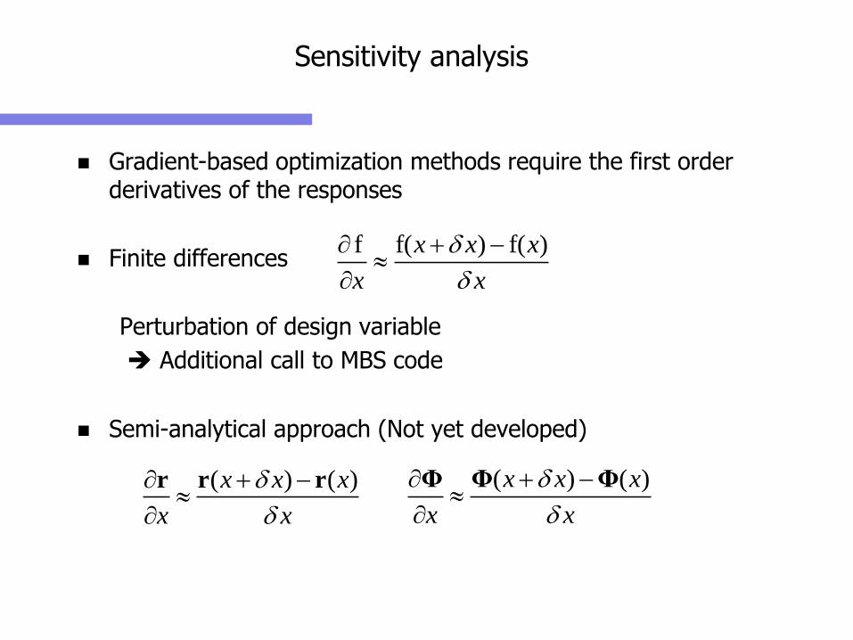
Gradient-based optimization methods require the first order derivatives of the responses
Finite differences
Perturbation of design variable
Additional call to MBS code
Semi-analytical approach (Not yet developed)
( ) ( )x x x
x x
d
d
r r r ( ) ( )x x x
x x
d
d
Φ Φ Φ
f f( ) f( )x x x
x x
d
d
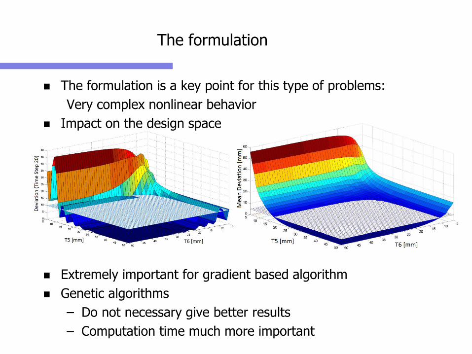
The formulation
The formulation is a key point for this type of problems:
Very complex nonlinear behavior
Impact on the design space
Extremely important for gradient based algorithm
Genetic algorithms
– Do not necessary give better results
– Computation time much more important
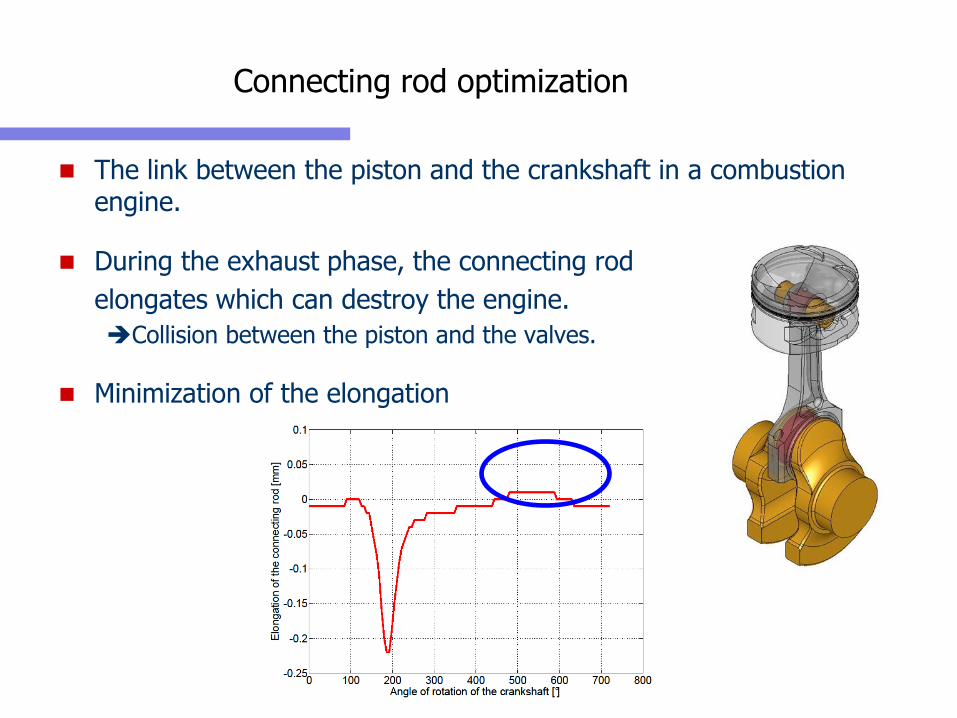
Connecting rod optimization
The link between the piston and the crankshaft in a combustion engine.
During the exhaust phase, the connecting rod
elongates which can destroy the engine.
Collision between the piston and the valves.
Minimization of the elongation
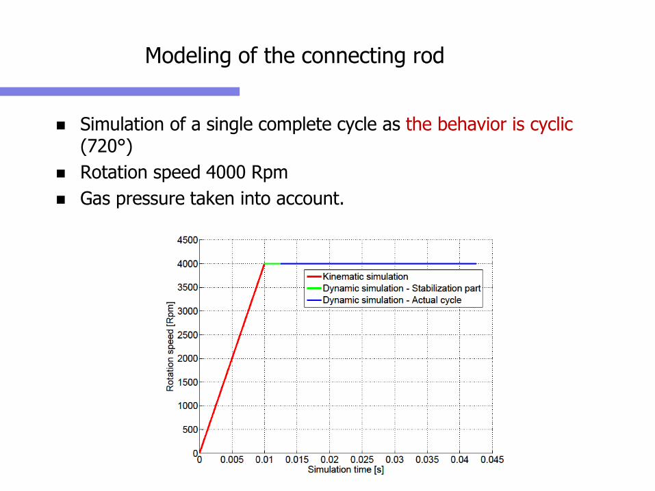
Simulation of a single complete cycle as the behavior is cyclic (720°)
Rotation speed 4000 Rpm
Gas pressure taken into account.
Modeling of the connecting rod
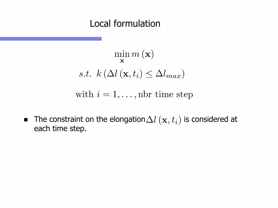
Local formulation
The constraint on the elongation is considered at each time step.
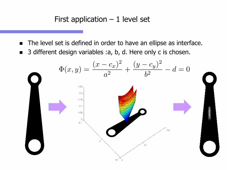
First application – 1 level set
The level set is defined in order to have an ellipse as interface.
3 different design variables :a, b, d. Here only c is chosen.
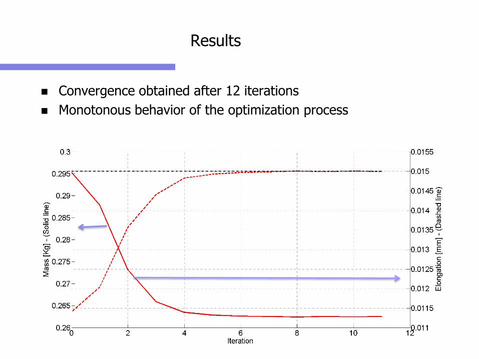
Results
Convergence obtained after 12 iterations
Monotonous behavior of the optimization process
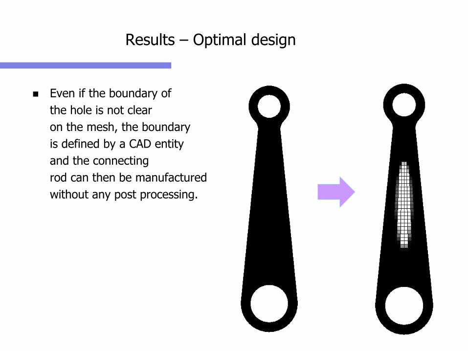
Results – Optimal design
Even if the boundary of
the hole is not clear
on the mesh, the boundary
is defined by a CAD entity
and the connecting
rod can then be manufactured
without any post processing.
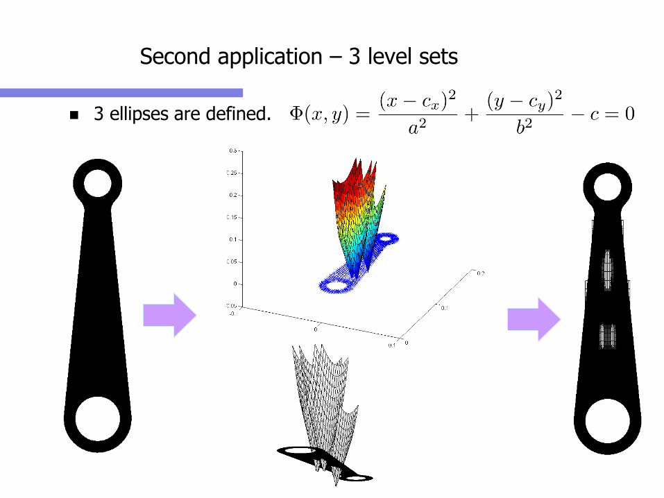
3 ellipses are defined.
Second application – 3 level sets
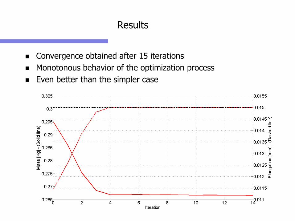
Results
Convergence obtained after 15 iterations
Monotonous behavior of the optimization process
Even better than the simpler case
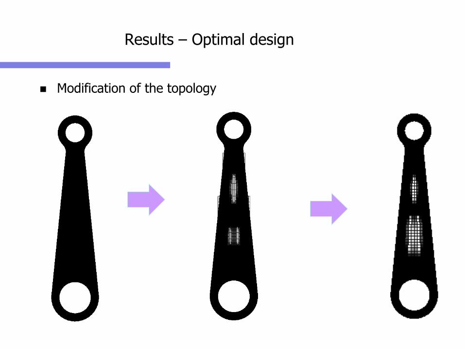
Results – Optimal design
Modification of the topology
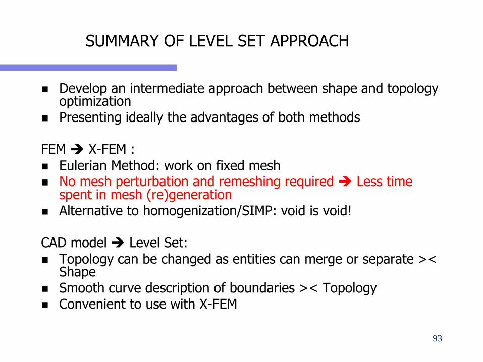
Develop an intermediate approach between shape and topology optimization
Presenting ideally the advantages of both methods
FEM X-FEM :
Eulerian Method: work on fixed mesh No mesh perturbation and remeshing required Less time
spent in mesh (re)generation Alternative to homogenization/SIMP: void is void!
CAD model Level Set:
Topology can be changed as entities can merge or separate >< Shape
Smooth curve description of boundaries >< Topology Convenient to use with X-FEM
SUMMARY OF LEVEL SET APPROACH
93
Shape and Topology Optimization of Lightweight Automobile Transmission Components
P. Duysinx, G. Virlez, S. Bauduin, E. Tromme
LTAS - Aerospace and Mechanical Engineering Department -University of Liège
N. Poulet
JTEKT Torsen Europe, Belgium
94
OUTLINE
Introduction & motivation
Modelling of Torsen Differential
Design approach using combined topology and shape optimization
Topology optimization
Shape optimization
– 2D shape
– 3D shape
Conclusion & Perspectives
95
MODELLING OF JTEKT DIFFERENTIAL
96
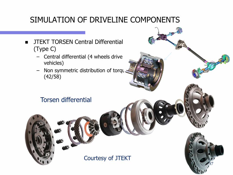
JTEKT TORSEN Central Differential (Type C)
– Central differential (4 wheels drive vehicles)
– Non symmetric distribution of torque (42/58)
SIMULATION OF DRIVELINE COMPONENTS
Torsen differential
Courtesy of JTEKT97
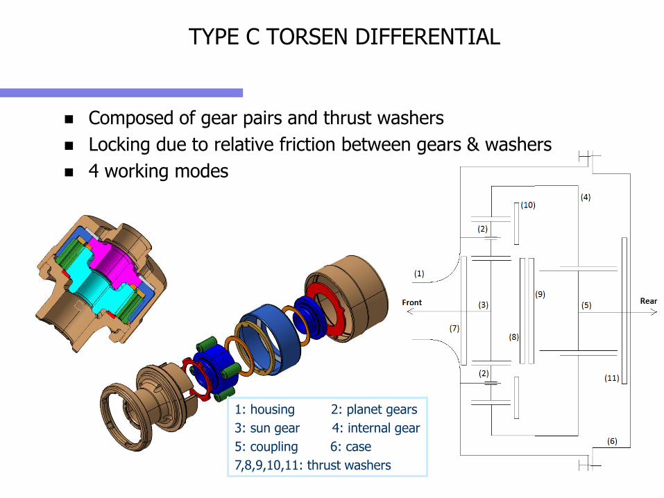
TYPE C TORSEN DIFFERENTIAL
Composed of gear pairs and thrust washers
Locking due to relative friction between gears & washers
4 working modes
1: housing 2: planet gears
3: sun gear 4: internal gear
5: coupling 6: case
7,8,9,10,11: thrust washers
OPTIMIZATION OF DIFFERENTIAL HOUSING
The goal of the work is to propose and validate a design methodology of transmission components including topology optimization and shape optimization
The methodology will be validated on the optimization of the housing of the type-C Torsen differential
Different steps will be carried out:
– Specifications
– Modelling
– Topology optimization
2D / 3D
– Shape optimization:
2D / 3D / dynamic loading 99
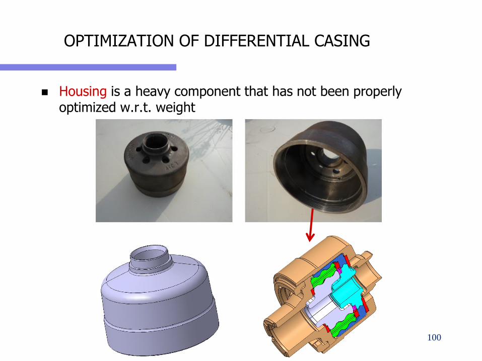
OPTIMIZATION OF DIFFERENTIAL CASING
Housing is a heavy component that has not been properly optimized w.r.t. weight
100

OPTIMIZATION OF TRANSMISSION COMPONENTSA HIERARCHICAL APPROACH
101
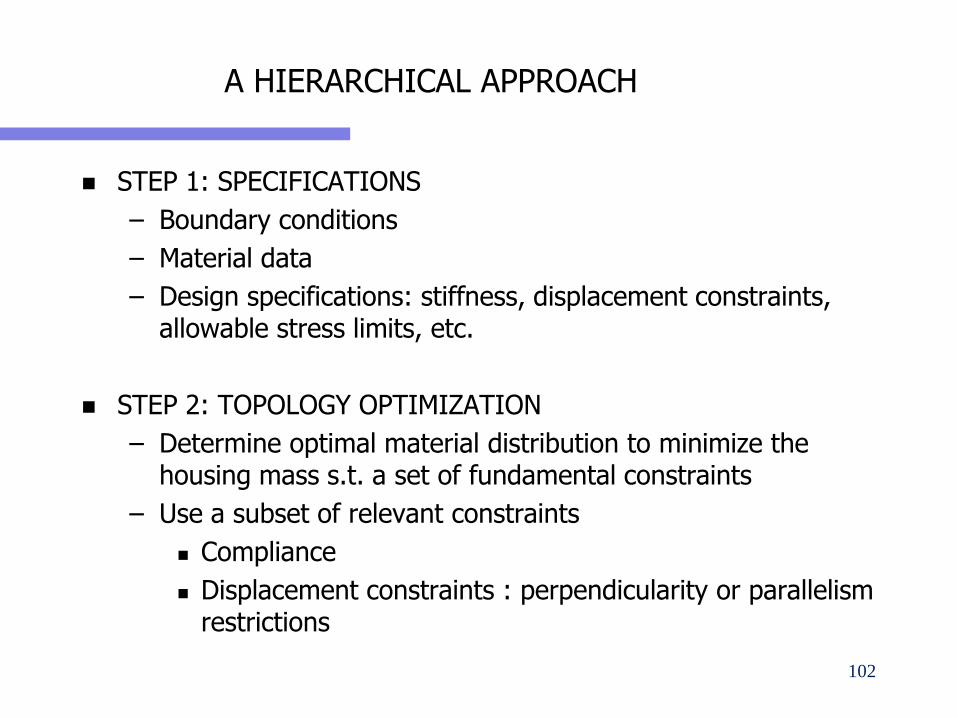
A HIERARCHICAL APPROACH
STEP 1: SPECIFICATIONS
– Boundary conditions
– Material data
– Design specifications: stiffness, displacement constraints, allowable stress limits, etc.
STEP 2: TOPOLOGY OPTIMIZATION
– Determine optimal material distribution to minimize the housing mass s.t. a set of fundamental constraints
– Use a subset of relevant constraints
Compliance
Displacement constraints : perpendicularity or parallelism restrictions
102
A HIERARCHICAL APPROACH
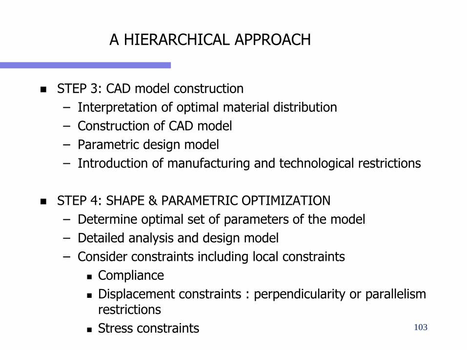
STEP 3: CAD model construction
– Interpretation of optimal material distribution
– Construction of CAD model
– Parametric design model
– Introduction of manufacturing and technological restrictions
STEP 4: SHAPE & PARAMETRIC OPTIMIZATION
– Determine optimal set of parameters of the model
– Detailed analysis and design model
– Consider constraints including local constraints
Compliance
Displacement constraints : perpendicularity or parallelism restrictions
Stress constraints 103
A HIERARCHICAL APPROACH
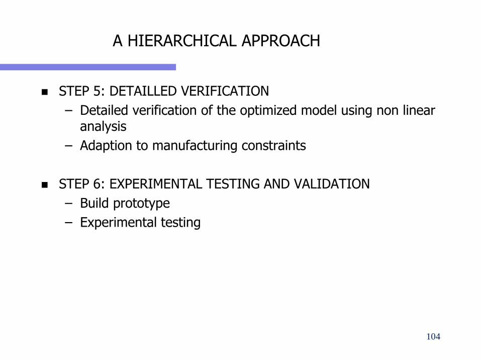
STEP 5: DETAILLED VERIFICATION
– Detailed verification of the optimized model using non linear analysis
– Adaption to manufacturing constraints
STEP 6: EXPERIMENTAL TESTING AND VALIDATION
– Build prototype
– Experimental testing
104
TOPOLOGY OPTIMIZATION
105
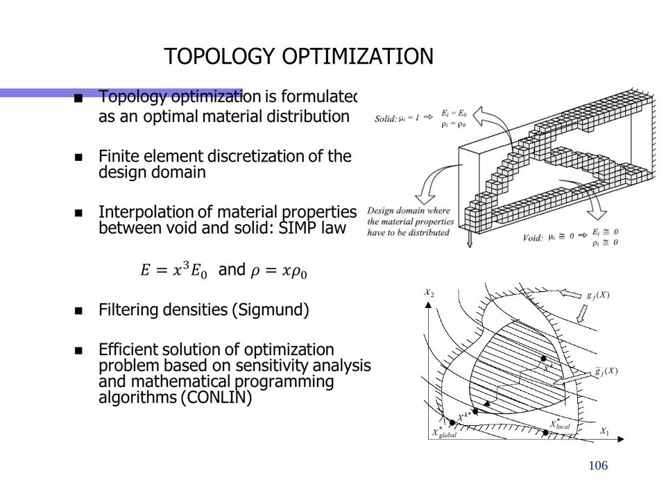
TOPOLOGY OPTIMIZATION
106
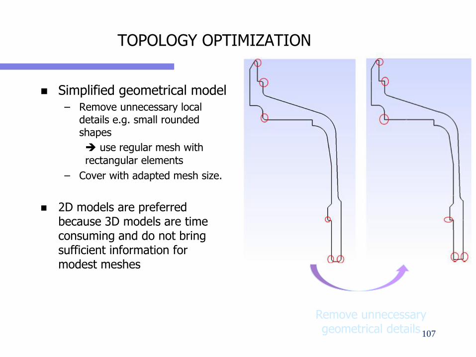
TOPOLOGY OPTIMIZATION
Simplified geometrical model– Remove unnecessary local
details e.g. small rounded shapes
use regular mesh with
rectangular elements
– Cover with adapted mesh size.
2D models are preferred because 3D models are time consuming and do not bring sufficient information for modest meshes
Remove unnecessary geometrical details107
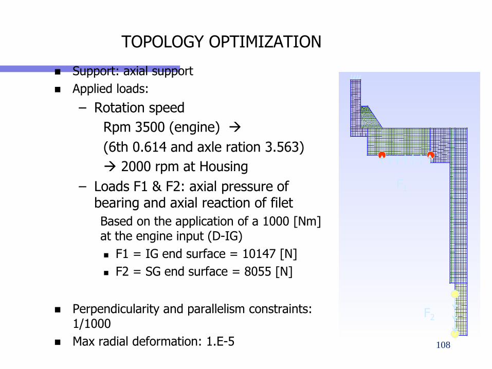
TOPOLOGY OPTIMIZATION
Support: axial support
Applied loads:
– Rotation speed
Rpm 3500 (engine)
(6th 0.614 and axle ration 3.563)
2000 rpm at Housing
– Loads F1 & F2: axial pressure of bearing and axial reaction of filet
Based on the application of a 1000 [Nm] at the engine input (D-IG)
F1 = IG end surface = 10147 [N]
F2 = SG end surface = 8055 [N]
Perpendicularity and parallelism constraints: 1/1000
Max radial deformation: 1.E-5
F1
F2
108
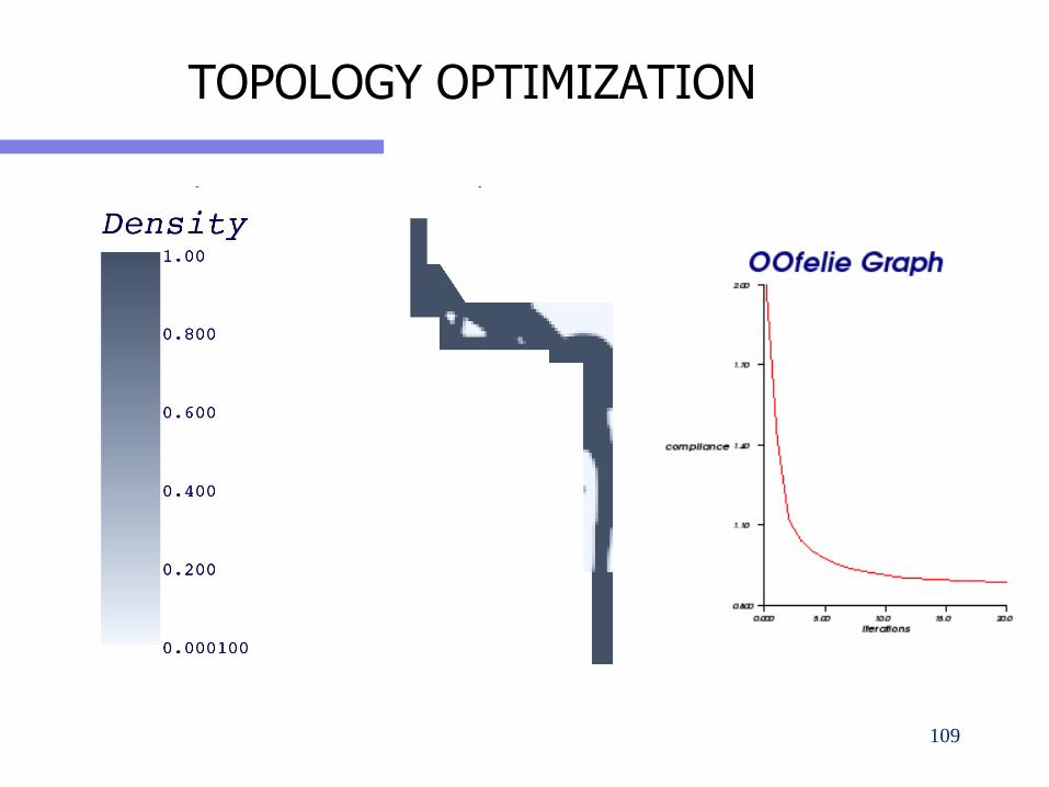
TOPOLOGY OPTIMIZATION
Topology optimization results
109
2D SHAPE OPTIMIZATION
110
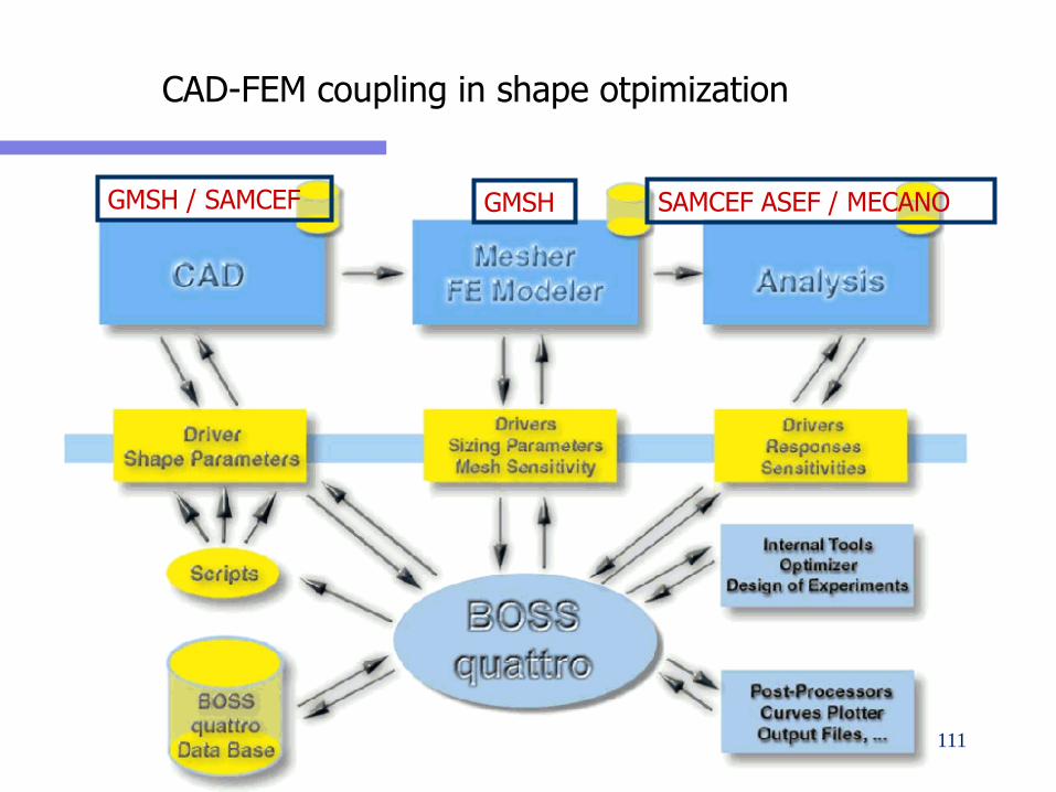
CAD-FEM coupling in shape otpimization
GMSH / SAMCEF GMSH SAMCEF ASEF / MECANO
111
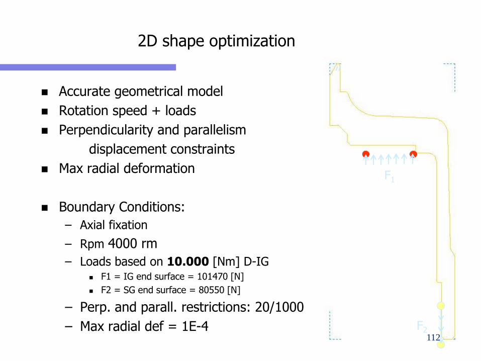
2D shape optimization
Accurate geometrical model
Rotation speed + loads
Perpendicularity and parallelism
displacement constraints
Max radial deformation
Boundary Conditions:
– Axial fixation
– Rpm 4000 rm
– Loads based on 10.000 [Nm] D-IG F1 = IG end surface = 101470 [N]
F2 = SG end surface = 80550 [N]
– Perp. and parall. restrictions: 20/1000
– Max radial def = 1E-4
F1
F2112
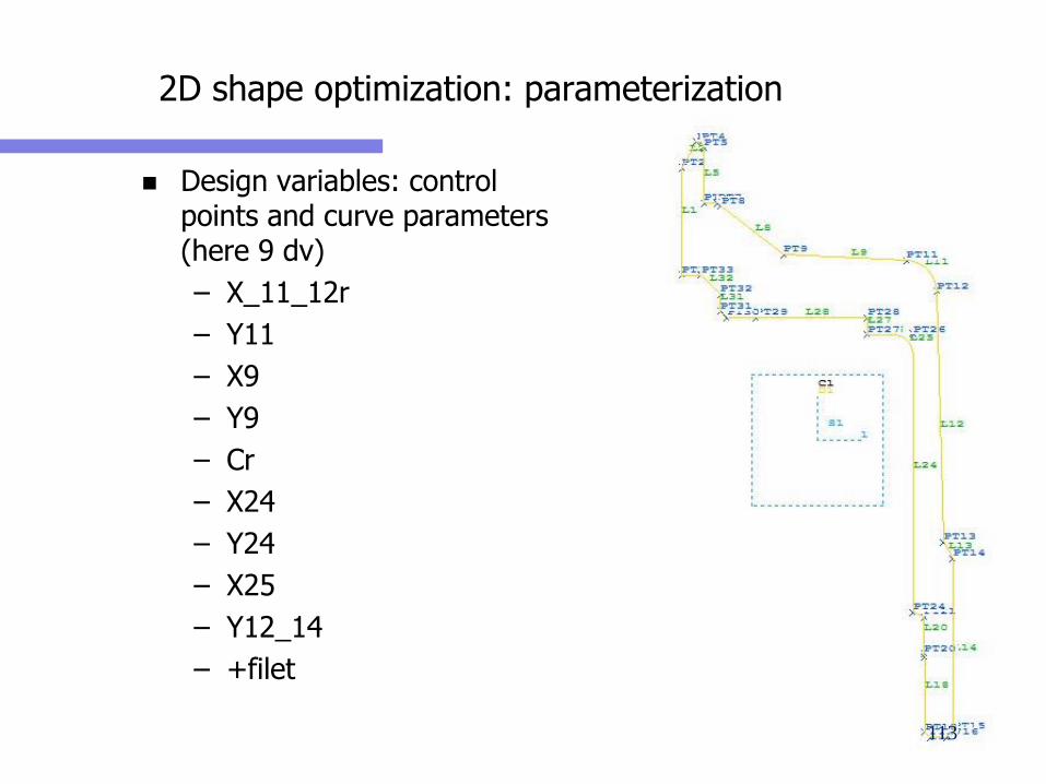
2D shape optimization: parameterization
Design variables: control points and curve parameters (here 9 dv)
– X_11_12r
– Y11
– X9
– Y9
– Cr
– X24
– Y24
– X25
– Y12_14
– +filet
113
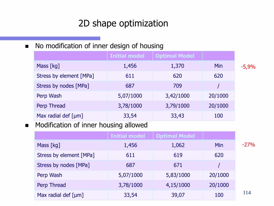
2D shape optimization
No modification of inner design of housing
Modification of inner housing allowed
Initial model Optimal Model
Mass [kg] 1,456 1,370 Min
Stress by element [MPa] 611 620 620
Stress by nodes [MPa] 687 709 /
Perp Wash 5,07/1000 3,42/1000 20/1000
Perp Thread 3,78/1000 3,79/1000 20/1000
Max radial def [µm] 33,54 33,43 100
Initial model Optimal Model
Mass [kg] 1,456 1,062 Min
Stress by element [MPa] 611 619 620
Stress by nodes [MPa] 687 671 /
Perp Wash 5,07/1000 5,83/1000 20/1000
Perp Thread 3,78/1000 4,15/1000 20/1000
Max radial def [µm] 33,54 39,07 100
-5,9%
-27%
114
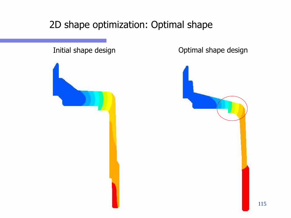
2D shape optimization: Optimal shape
Optimal shape designInitial shape design
115
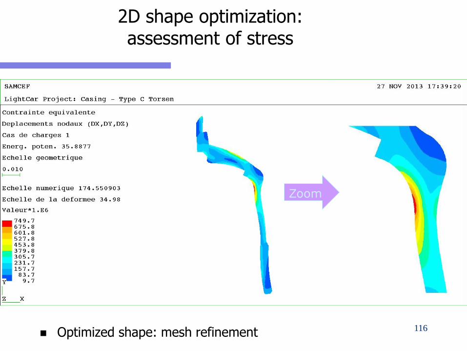
2D shape optimization: assessment of stress
Optimized shape: mesh refinement
Zoom
116
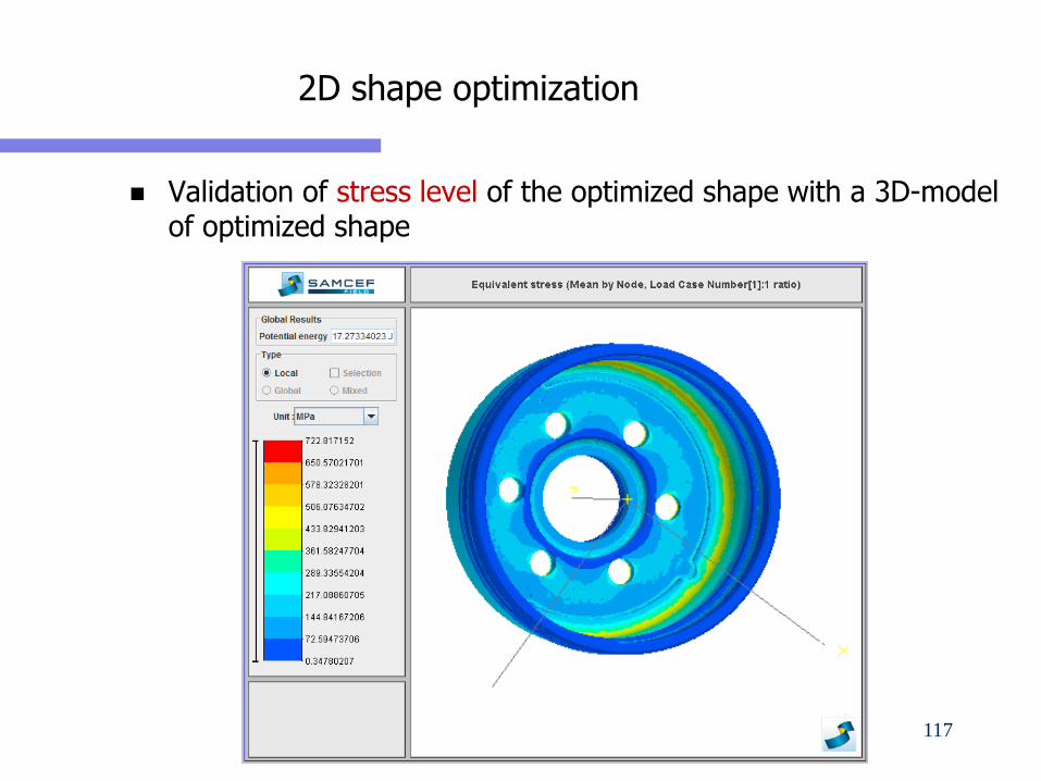
2D shape optimization
Validation of stress level of the optimized shape with a 3D-model of optimized shape
117

3D SHAPE OPTIMIZATION
118
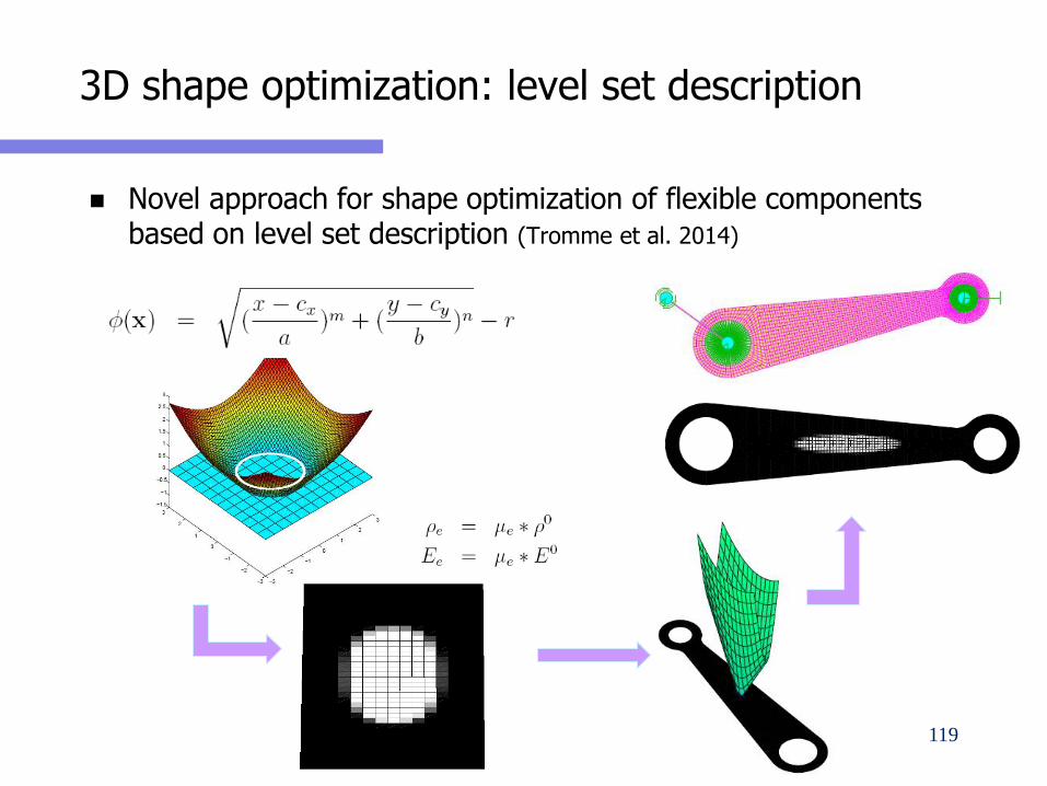
3D shape optimization: level set description
Novel approach for shape optimization of flexible components based on level set description (Tromme et al. 2014)
119
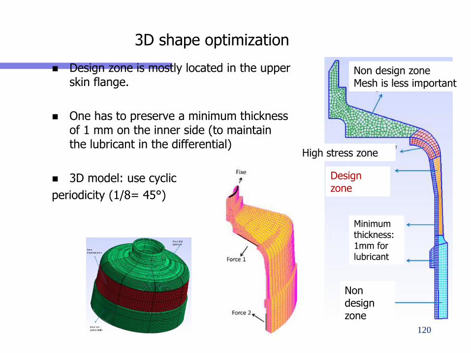
3D shape optimization
Design zone is mostly located in the upper skin flange.
One has to preserve a minimum thickness of 1 mm on the inner side (to maintain the lubricant in the differential)
3D model: use cyclic
periodicity (1/8= 45°)
Minimum thickness: 1mm for lubricant
Non design zone
Design zone
High stress zone
Non design zoneMesh is less important
120
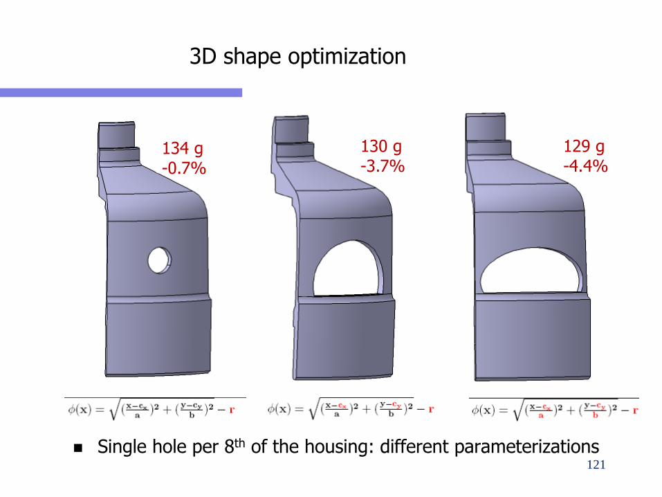
3D shape optimization
Single hole per 8th of the housing: different parameterizations
134 g-0.7%
130 g-3.7%
129 g-4.4%
121
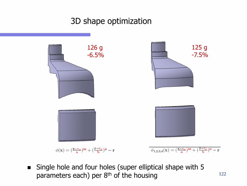
3D shape optimization
Single hole and four holes (super elliptical shape with 5 parameters each) per 8th of the housing
126 g-6.5%
125 g-7.5%
122
CONCLUSIONS& PERSPECTIVES
123
CONCLUSIONS
Great interest of industrial designers in using structural optimization to weight reduction in automotive components
Successful application of topology and shape optimization to design cycle of driveline components.
Approach validated on several components from real automotive sector(JTEKT TORSEN and TOYOTA MOTOR)
One major output of optimization is also to be able to find innovative and feasible solutions in complex problems
Nice and flexible approach of level set in solving shape optimization on real life / industrial problems including 3D models.– Especially great interest in optimizing dead geometrical models (not
necessary to have the parametric model)
124
PERSPECTIVES
Prototyping of the optimized shape
– On going task: delayed because the housing was so stiff that the test bed was damaged…
– Testing on JTEK TORSEN test bed.
Integrated design chain is still to be built:
– Interpretation of topology results (see Rasmussen, Bendsoe, Olhoff, 1992 paper…)
– ‘Automatic’ or a least assisted reconstruction of CAD model is still to be done…
125
PERSPECTIVES
Topology optimization:
– Stress constraints are essential for mechanical applications in real life problem
– Compliance problems should be at least complemented by displacement constraints
– 3D problems have to carefully investigated
Shape optimization:
– Non linear analysis should bring valuable information
– Old problems still pending: CPU time? Mesh problems?
126
Recommended