Eastern Illinois UniversityThe Keep
Masters Theses Student Theses & Publications
2018
Investigating the Impact of Foreign DirectInvestment on Domestic Investment in Sub-Saharan Africa: A Case Study of Kenya and SouthAfricaGeorge AnamanEastern Illinois UniversityThis research is a product of the graduate program in Economics at Eastern Illinois University. Find out moreabout the program.
This is brought to you for free and open access by the Student Theses & Publications at The Keep. It has been accepted for inclusion in Masters Thesesby an authorized administrator of The Keep. For more information, please contact [email protected].
Recommended CitationAnaman, George, "Investigating the Impact of Foreign Direct Investment on Domestic Investment in Sub-Saharan Africa: A CaseStudy of Kenya and South Africa" (2018). Masters Theses. 3715.https://thekeep.eiu.edu/theses/3715

The Graduate School� E..<\5rn\,'IJ lui1'X'l!S Us1VFASITY •
Thesis Maintenance and Reproduction Certificate
FOR: Graduate candidates Completing Theses in Partial Fulfillment of the Degree Graduate Faculty Advisors Directing the Theses
RE: Preservation, Reproduct.ion, and Distribution of Thesis Research
Preserving, reproducing, and distributing thesis research is an important part of Booth Library's responsibility to
provide access to scholarship. In order to further this goal, Booth Library makes all graduate theses completed as
part of a degree program at Eastern Illinois University available for personal study, research, and other not-for
profit educational purposes. Under 17 U.S.C. § 108, the library may reproduce and distribute a copy without
infringing on copyright; however, professional courtesy dictates that permission be requested from the author
before doing so.
Your signatures affirm the following:
• The graduate candidate is the author of this thesis.
•The graduate candidate retains the copyright and intellectual property rights associated with the original
research, creative activity, and intellectual or artistic content of the thesis.
•The graduate candidate certifies her/his compliance with federal copyright law (Title 17 of the U.S. Code) and
her/his right to authorize reproduction and distribution of all copyrighted materials included in this thesis.
•The graduate candidate in consultation with the faculty advisor grants Booth Library the nonexclusive, perpetual
right to make copies of the thesis freely and publicly available without restriction, by means of any current or
successive technology, including but not limited to photocopying, microfilm, digitization, or internet.
•The graduate candidate acknowledges that by depositing her/his thesis with Booth Library, her/his work is
available for viewing by the public and may be borrowed through the library's circulation and interlibrary loan
departments, or accessed electronically. The graduate candidate acknowledges this policy by indicating in the
following manner:
V Yes, I wish to make accessible this thesis for viewing by the public
___ No, I wish to quarantine the thesis temporarily and have included the Thesis Withholding Request Form
•The graduate candidate waives the confidentiality provisions of the Family Educational Rights and Privacy Act
(FERPA) (20 U. S. C. § 1232g; 34 CFR Part 99) with respect to the contents of the thesis and with respect to
information concerning authorship of the thesis, including name and status as a student at Eastern Illinois
University. I have conferred with my graduate faculty advisor. My signature below indicates that I have read and
agree with the above statements, and hereby give my permission to allow Booth Library to reproduce and
my thesis. My adviser's signature indicates concurrence to �l'.ld distribute the thesis.
Graduate candidate Signature
Gsro�e. -1\rt=ttrrF;ry Printed Ne
M/\ -€ccno1-o;c.s Graduate Degree Program
Please submit in duplicate.
Faculty Adviser Signature
1t ' 1> E& \ R. � f}:Dt) t'\ Pri�ef �atj
w: Date

INVESTIGATING THE IMPACT OF FOREIGN DIRECT INVESTMENT ON DOMESTIC
INVESTMENT IN SUB-SAHARAN AFRICA: A CASE STUDY OF KENYA AND SOUTH AFRICA
(TITLE)
BY
GEORGE ANAMAN
THESIS
SUBMITTED IN PARTIAL FULFILLMENT OF THE REQUIREMENTS
FOR THE DEGREE OF
Master of Arts in Economics
IN THE GRADUATE SCHOOL, EASTERN ILLINOIS UNIVERSITY
CHARLESTON, ILLINOIS
2018 YEAR
I HEREBY RECOMMEND THAT THIS THESIS BE ACCEPTED AS FULFILLING
THIS PART OF THE GRADUATE DEGREE CITED ABOVE
£/g\\� �? THESIS COMMITTEE CHAIR DATE DEPARTMENT/SCHOOL DATE
OR CHAIR'$
G/�/;J I
THESIS COMMITTEE MEMBER DATE Tl l[SIS COMMITTEE MEMBER DATE
#J THESIS COMMITTEE I DATE THESIS COMMITTEE MEMBER DATE

INVESTIGATING THE IMP ACT OF FOREIGN DIRECT INVESTMENT ON
DOMESTIC INVESTMENT IN SUB-SAHARAN AFRJCA: A CASE STUDY OF
KENYA AND SOUTH AFRJCA
George Anaman
Eastern Illinois University
2018
Thesis Committee
Dr. A. Desire Adorn (Advisor)
Dr.:tvfuktiUpadhyay
Dr. Ali Moshtagh
Abstract
In the progression towards economic growth, countries consider investment as a
critical feature in raising productivity levels by boosting technological progress and
reducing the unemployment rate. In recent years, the government of South Africa and
Kenya have both enacted policies to entice Foreign Direct Investment (FDI) in the view
of creating more jobs and bolstering the economy. However, in the bid to attract these
foreign investors, FDI may either end up complementing or stifling local investments
over time. From this perspective, the objective of the study is to investigate the impact of
FDI on Domestic Investments in Sub -Saharan Africa (SSA) with an individual
investigation on Kenya and South Africa. Analyzing annual series of data from 1972 -
2011 , our Pooled OLS results shows that FDI has no impact on domestic investment in
SSA countries. Using time series to dig deeper to establish the relationship between FDI
and domestic investment in both countries, we found out that FDI does not impact
domestic investment in both the Short -run and the long -run period for Kenya but has a
crowding -out effect in South Africa only in the short -run period. However, economic
growth, inflation rate, trade openness and exchange rate were critical drivers of domestic
investment in SSA countries.

Acknowledgement
I would like to foremost thank the almighty God for how far he has brought me in
life. A special acknowledgment goes to my supervisor Dr. A. Desire Adorn for his
immerse support, guidance, and effort in assisting me to complete my thesis on time. I
also like to thank the thesis committee members Dr. Mukti Upadhyay and Dr. Ali
Moshtagh for their thoughtful inputs in nourishing my paper.
To my parents, Mr. Francis Anaman and Ms. Augustina Agyemang, I say a big
thank you for encouraging and imbibing in me the "can do" spirit. In addendum, my
sincere gratitude goes to Drs. Nina Banks, Michelle Johnson, Ned Searles, and Kurt
Olausen, Mr & Mrs. Ofori, Mr. Eric Anaman, Estella Anaman, Omel Anaman, Eric
Thomford, Bobbie Hunter, Samuel Eliason and my host parents Mr & Mrs. Trueblood for
their immeasurable support and care throughout my journey at EIU.
Finally, I would like to thank my colleagues especially Temiyemi Akinsuyi and
Tinuke Laguda for cheering me on during difficult moments of my life.
Table of Contents
CHAPTER ONE: Introduction . . . . . . . . . . . . . . . . . . . . . . . . . . . . . . . . . . ..... . . . . . . .. . . . . . . . . . . . . ... . . . . . ... I
I . I . Justification of the Study . . . . . . . . . . . . .. . . . . . . . . .. . . ... . . . . . . . . . . ..... . . . . . . . . . . . . . . . . . ... . . ... . .4 I .2. Objective of the Research . . . . . . . . . . . ... . . . . . . . . . . . . . . . . ..... . . . ... . . . . . . . . . . . . . . . . . . . . . . . . ...... 5 I .3 . Hypothesis . . . . . . . . . . . . . . . . . . . . . . . . . . . . . . . . . . . . . . . . . . . . . . . . . . . . . . . . . . . . . . . . . . . . . . ... ... . . . . . . . . . .... 6 I .4. Organization of the study . . . . . . . . . . . . . . . . . . . . . . . . . ... . . . . . . . . . . . . . . . . . . . . . . . ... . . . . . . . . ..... . . ... 6
CHAPTER TWO: Literature Review . . . . . . ... . . . . . . . . . . . . . . . . . . . ... . . . . . . . . . . . . . . ...................... 7
CHAPTER THREE: Background and Trends in Domestic and Foreign Investment. . .... 2I
3 . 1 . Background of Kenya ................................................................................................. 21
3.2. Background of South Africa . . . . . . . . . . . . . . . . . . . . . . . . . . . . . . . . . . . . . . . . . . . . . . . . .. . . . . . . . . . . . . . . . . 22
3.3. Trends in Domestic Investment in Kenya and South Africa . . . . . . . . . . . . . . . . . . . . . .......... 24
3.4. Trends of FDI in SSA . . . . . . . . . . . . . . . . . . . . . . . . . . . . . . . . . ... . . . . . . . . . . . . . . . . . . . . . . . .................. 26
3.5. Trends of FDI in Kenya and South Africa . . . . . . . . . . . . . . . . . . . . . . . . . . . . . . . . . . .................... 27
CHAPTER FOUR: Methodology and Data . . . . . . . . . . . . . . . . . . . . . . . . . . . . . . . . . . . ... . . . . . . . . . . . . . . .. 30
4. 1. Methodology . ... . . . . . . . . . ... . . . . . . . . . . . . . . . . . . . . . . . . . . . . . ... . . . . . . . . . . .. . ... . . . . . ................... 30
4. I. I Model Specification . . . . . . . . . . . . . . . . . . . . . . . . . . . . . . . . ... . . . . . . . .. . . . . . ......... ............ 31
4 . 1 .2 Theoretical and Empirical use ofVariables . . . . . . . . . . . . . . . . . . ......................... .33
4.2 Data . . . . . . . . . . . . . . . . . . . . . . . . . . . . . . . . . . . . . . . . . . . . . . . . . . . . . . . . . . . . . . . . . . . . . . . . . . . . . . . . ................... 37
4.2.1 Sources of data . . . . . . . . . . . . . . . . . . . . . . . . ... . . ... . . . . . . . . . . . . . . . . . . . . .. . . . .................. 39
CHAPTER FIVE: Discussion and Policy recommendation . . . . . . . . . . . .. . . . . . . . . ................ . .40
5 . 1 . Descriptive Statistics and Correlation Matrix . . . . . . . . . . . . . . . . . . . . . . . . . . . . . . . . . . . . . . . . ...... .40
5.2. Pooled OLS estimates ............................................................................. 42
5.3. Time series estimates for Kenya ............................................................ .48
5.3.l Estimation ofECM for Kenya . . . . . . . . . . . . . . . . . . . . . . . . . . . . . . . . . . . . . . . . . . . . . . . ....... 53
5.4. Time series estimates for South Africa . . . . . . . . . . . . . . . . .. . . . . . . . . . . . . . . . . . . . . . . . . . . . . . . . . . ... 56
5.4.1 Estimation ofECM for South Africa ... . . . . . . . . . ..... . . . . . . . ... ... ... . . . . . . . . . .... 60
5.5 Policy recommendation . . . . . . . . . . . . . . . . . . . . . . . . . . . . . . . . . . . . . . . . . . . . . . . . . . . . . . . . . . . . . . ... . . . .... 64
CHAPTER SIX: Conclusion . . . . . . . . . . . . . . . . . . . . .. . . . . . .. . . . . . . . . . . . . . . ... . . . . . . . . . . . . . . . . . ..... .... 66
References . . . . . . . . . . . . . . . . . . . . . . . . . . . . . . . . . . . . . ... ... . . . . . . . . . . . . . . . ... . . . . . . ... . . . . .... . . . . . . . . ....... 69
Appendix . . . . . . . . . . . . . . . . . . ... . . ... . . . . . . . . . . . .. .... . . . . . . .. .... . . ..... . . . . . . . . ..... . . . . . . . . . . ... . . .... 77

List of Figures
Figure l : Trends in Domestic Investment in Kenya and South Africa(% of GDP) . . . . . . . 25
Figure 2: Net FDI inflows in SSA, 1972 -201 1 , in Millions (USD) . . . . . . . . . . . . . . . . . . . . . . . . . . 26
Figure 3: Net FDI in Kenya and South Africa, 1972 -201 1 , in Millions (USD) . . . . . . . . . . . . 27

List of Tables
Table 5 . 1 : Descriptive Statistics for Kenya and South Africa . . . . . . . . . . . . . . . . . . . . . . . . . . . .. . . . . 41
Table 5.2: Correlation Matrix for Kenya and South Africa . . . . . . . . . . . . . . . . . . . . . . . . . . . . . . .... . .41
Table 5.3: Correlation Matrix of Independent Variables . . . . . . . . . . . . . . . . . . . . . . . . . . . . . . . . . . . . . . . 42
Table 5.4. Pooled OLS for Kenya & South Africa, 1972 - 201 1 . . . . . . . . . . . . . . . . . . . . . . . . . . . . .43
Table 5.5: Diagnostics Test for Pooled OLS . . . . . . . . . . . . . . . . . . . . . . . . . . . . . . . . . . . . . . . . . . . . . . . . . . . .46
Table 5.6: Model I adjusted for Heteroskedasticity (Pooled OLS) . . . . . . . . . . . . . . . . . . . . . ...... .47
Table 5.7: Unit root test for Kenya using ADF . . . . . . . . . . . . . . . . . . . . . . . . . . . . . . . . . . . . . . . . . . . . . . . . .48
Table 5.8: ADF test of Residuals for Kenya . . . . . . . . . . . . . . . . . . . . . . . . . . . . . . . . . . . . . . . . . . . . . . . . . . . . .48
Table 5.9: Long-run Relationship between FDI and Domestic Investment in Kenya . . . . . .49
Table 5.10: Diagnostic Tests for Long run Models for Kenya . . . . . . . . . . . . . . . . . . . . . . . . . . . . . . . . 52
Table 5. 1 1 : Short -run parsimonious regressions for South Africa . . . . . . . . . . . . . . . . . . . . . . . . . . . .53
Table 5.12: Diagnostic Tests for Short-run parsimonious regressions for Kenya . . . . . . . . . 56
Table 5.13: Unit root test for South Africa using ADF . . . . . . . . . . . . . . . . . . . . . . . . . . . . . . . . . . . . . . . . 56
Table 5.14: ADF test of Residuals for South Africa . . . . . . . . . . . . . . . . . . . . . . . . . . . . . . . . . . . . . . . . . . . . . 57
Table 5.15: Long-run Relationship between FDI and Domestic Investment in South
Africa . . . . . . . . . . . . . . . . . . . . . . . . . . . . . . . . . . . . . . . . . . . . . . . . . . . . . . . . . . . . . . . . . . . . . . . . . . . . . . . . . . . 58
Table 5.16: Diagnostic Tests for Long -run Models for South Africa . . . . . . . . . . . . . . . . . . . . . ... 60
Table 5.17: Short-run parsimonious regressions for South Africa . . . . . . . . . . . . . . . . . . . . . . . . . . . 61
Table 5.18: Diagnostic Tests for Short-run parsimonious regressions . . . . . . . . . . . . . . . .. . . . . . . 63


CHAPTER ONE
INTRODUCTION
According to the annual report issued by the United Nations Development
Program (UNDP), Human Development Indicators (HDI1) for Sub-Saharan Africa (SSA)
countries are recorded to be the lowest relative to the rest of the world. The region
accounted for an average HDI index of 0.475 among regions of the world (UNDP, 2013).
The World Bank indicators show that the region has half of its population below the
poverty line with a headcount ratio at $1.25 a day (PPP) (World Bank, 2010; Demelew,
2014). Also, SSA countries have a Gross National Income (GNI) per capita, five times
lower than the world average with a per capita income of $2,010 (UNDP, 2013).
In the progression towards economic growth, countries consider investment as a
crucial feature in raising productivity levels by boosting technological progress and
reducing the unemployment rate. It bolsters long-run capital accumulation as investment
creates new capital goods and increases the productive capacity of countries. The
Investment Promotion Act2 (IP A, 2004) defines investment as the contribution of local or
foreign capital by an investor, including the creation of, or the acquisition of business
assets by or for business enterprises, and includes expansion, restructuring, improving or
rehabilitating of a business enterprise. Investment of a country may be domestic or
foreign.
The modem economy has investment as one of the four pillars -along with
government spending, private consumption, and trade-ofthe macroeconomic
1 The United Nations Development Program (UNDP) issues yearly report on HDI by compiling a
multidimensional poverty indicators including education, health and income per capita.
2 The IPA, 2004 is an ACT enacted by the Kenyan Parliament to promote and facilitate investment by
assisting investors in obtaining the Licenses necessary to invest and by providing other assistance and
incentives and for related purposes.
1

expenditure model. It has empirically be revealed that countries with high investment
levels have higher economic growth and that investment is the nub of an economy and
any instability in investment levels have significant effects on the long -term growth path
of the economy (Guma, 2013).
Domestic investment can generally be referred to as the investment in the
companies and products of one's own country rather than in those of foreign countries.
Domestic investment comprises of private and public investment. Private investment can
be defined as investment by private businesses for the motive of generating profit whiles
public investment refers to investment by the government sector primarily, but not
exclusively, on social and core economic infrastructure (Matsila, 2014). Domestic
investment is one of the most important components of economic growth that countries
consider as the main engine of the economic cycle. Recent theories on the nee-classical
growth model as well as theories of endogenous growth has emphasized the role of
domestic investment in economic growth such as capital spending on new projects in the
sectors of public utilities and infrastructure like roads projects, housing, electricity
extensions, as well as social development in the areas of health, education, and
communication projects among others.
Foreign direct investment (FDI) on the other hand can be defined as an
investment made to acquire lasting interest in enterprises operating outside of the
economy of the investor (UNCTAD, 2014).
For the last 50 years, FDI has propelled both theoretical and empirical debate on
the grounds of its costs and benefits to the host countries. It is an established facts in FDI
literature that one of the rudimentary rationale encouraging developing countries to
2

welcome FDI is the promise that these foreign firms would come along with capital
which beforehand was not available in the recipient countries and equip the domestic
economies with new potentials for economic growth and development (Ahmed et al.,
2015). Other developing countries are emulating South East Asian countries in light of
the positive and crucial role played by FDI in their economic development and growth.
Following the surge ofFDI to the developing economies, a major controversial
issue on the impact ofFDI on recipient country is whether FDI complements or substitute
domestic investment. The effe.ct on domestic investment after liberalizing FDI may vary
depending on the domestic investment environment and the previous trade regime of the
host country (Acar et al., 201 2). FDI could displace domestic investors with less
technological and financial might. That is, if an inward flow of foreign capital enters
sectors that are already flooded with domestic firms (or firms already producing for
export markets), market stealing effect will be evident. Many studies done after the mid-
1 990s have exposed that the productive performance of domestic firms has been
stagnating and most of the domestic firms are not able to meet their objectives due to
competition from their foreign counter parts (Teal, 1 999). The contribution to total capital
formation of such FDI is likely to be less than the FDI flow itself (Agosin and Machado,
2005). On the flip side of the argument� FDI could complement or have a positive
spillover through the diffusion of new technological know-how, managerial skills, market
and labor skills.
In light of the theoretical ambiguity, this paper seeks to analyze if the presence of
Multinational corporations (MNCs) stimulates new downstream or upstream domestic
investment that would not have taken place in their absence or whether they end up
3

displacing domestic investors pre-emptying their investment opportunities in SSA with a
focus on Kenya and South Africa. If our empirical analyses were to show that indeed FDI
crowds out domestic investment, there would be a good reason to question its benefit for
recipient SSA countries particularly Kenya and South Africa (Agosin and Machado,
2005). This is because if FDI crowds out the domestic investment, then the growth of
domestic capital stock will be squeezed.
Kenya and South Africa have been landmarked to be part of Africa's fastest-growing
economies, and over the last few decades have attracted a large amount ofFDI. It is
therefore imperative to examine the effects ofFDI on domestic investment in these
countries.
1 . 1 Justification of the Study
The significance of this study is based on the score that among the research works
conducted on FDI, domestic investment and economic growth in Sub-Saharan Africa
(Morrissey, 2012; Ndikumana and Verick, 2008; Ndikumana, 2003; Dupasquier and
Osakwe, 2006) just a few have examined the impact ofFDI on domestic investment in
Kenya and South Africa on a time series analysis. A distinguishing feature of this study is
the use of FD I as the determinant of domestic investment in both countries. This work
will give an in-depth knowledge of the workings of FDI and its rippling effect on the
domestic firms of these two countries. In addition, this will assist the government in
designing or having a second look at the FDI policy framework to ensure that any
negative effect of foreign investment on the domestic economy is curtailed before it is too
late.
4

Also, domestic investors and other stakeholders will benefit from the information
that will be revealed in this work so as to adopt to the necessary measures and techniques
to ensure longevity on the market if FDI is causing substitutability effect or
complementarity effect. The proper understanding of the impact ofFDI on the domestic
market will better equip both local and foreign investors on initiatives to take for the
betterment of all. Equally, the study could set off the mark for further research into the
effect ofFDI on other macroeconomic variables or on this same variable to bring on the
table other potent factors that may be in play.
1 .2 Objective of the Research
In recent times, the government of South Africa and Kenya have both enacted
policies to entice FDI with the rationale of creating more jobs and bolstering the
economy. However, higher FDI inflows may also have a negative impact on the local
economy through crowding out of the domestic investment.
The objective of the study is to analyze the impact ofFDI on domestic investment
in SSA countries using pooled OLS. We then conduct an individual time series analyses
of the effect of FDI on domestic investment in Kenya and South Africa using annual data
from 1972- 201 1 .
To achieve this aim, this research work specifically analyses the trends in domestic
investment and FDI from 1972 to 201 1 . We then estimate the impact ofFDI on domestic
investment in SSA on the pooled level and individual investigations of the two countries
on the time series level.
5

1.3 Hypothesis
This study seeks to empirically test the following hypothesis based on research
objectives:
H0: FDI has no impact on domestic investments.
H1: FDI has an impact on domestic investments.
1 .4 Organization of the Study
For the purpose of this study, we have divided the paper into 6 chapters. The rest
of the project is organized as follows. Chapter 2 presents a comprehensive survey of
literature and review ofFDI and domestic investment across the globe. Chapter 3 gives a
background information on Kenya and South Africa together with trends in domestic and
foreign investment.
Chapter 4 describes the methodology and data used in the study. The next chapter
discusses our empirical results with policy recommendations. Lastly, chapter 6 concludes
with the main findings of the study.
CHAPTER TWO
LITERATURE REVIEW
6

Empirics on the relationship between FDI and domestic investment of the
recipient country have been evinced to be mixed. Conducting a study on the crowding
out effects ofFDI on domestic investment in China, Li-jun and Hong-qin (2006) made
use of data dating from 1985 - 2003 to aid them in their analyzes. The study revealed that
the effect ofFDI on economic growth is not certain from the capital formation
perspective. Thus, it is dependent on whether FDI crowds out or crowds in domestic
investment in its entirety. The result showed evidence of a simultaneous crowding in and
crowding out effects of FDI on domestic investment but in collective terms, there is a
"net crowding -in" effect. Additionally, Tang et al., (2008) adopting multivariate VAR
system with error correction model (ECM) and the innovation accounting (variance
decomposition and impulse response function analysis) technique investigating the causal
link between FDI, domestic investment and economic growth in China over the period
1988 -2003 also found that while there is a bi-directional causality from FDI to domestic
investment and to economic growth, there is only one-way directional causality from FDI
to domestic investment and to economic growth. FDI was found to rather have a positive
spillover effect on domestic investment. Thus, FDI has not only bolstered in overcoming
the shortage of capital but it has also promoted economic growth by complementing
domestic investment in the country of China.
Utilizing the model of Fry (1995), Ying-Jun (2006) investigated the influence of
FDI on Chinese domestic investment. The study showed a remarkable crowding -in
effect ofFDI on domestic investment as a whole. Further analysis of the study also
showed that FDI effect varied across the Chinese region. That is, FDI exhibited crowding
in effect and crowding out in the East part of China while its positive externalities are
7

limited or insignificant or uncertain in Central China. But in the west, the effect of FDI is
discreet in most provinces or even outcompeting domestic investment in some districts.
Using quarterly and more up to date data covering periods subsequent to the
Asian financial crisis, Deok-Ki Kim and Seo (2003) employed a vector autoregression
(VAR) model to estimate the dynamic relationship between the inflow ofFDI, economic
growth and domestic investment in Korea covering the period of 1985 to 1999. This
technique according to Deok-Ki et al., (2003) gives plausible structural techniques and in
addition employed impulse response and variance decomposition techniques to examine
dynamic interactions ofFDI, economic growth and domestic investment. The output of
their correlation matrix of residuals confirmed that shocks to FDI are contemporaneously
orthogonal to domestic investment. To capture the post-financial crisis period, they
included a dummy variable to capture if there is any possible significance of this period
in their estimation. The study revealed that, while FDI effect on the growth rate of output
is temporary, it shock (FDI) could have a permanent effect on the level of output. FDI
shock had a negative but insignificant effect on domestic investment. However, if
domestic investment is allowed to be contemporaneously most endogenous, the response
of domestic investment to the shock of FDI becomes positive, albeit statistically
insignificant for the overall sample period for the study. FDI also responded positively to
domestic investment shocks while the response was negative over the entire sample
period. The reason accounted was that, in the pre-crisis era, a positive shock to domestic
shock is taken as an opportunity for foreign investors to flow in their resources in Korea.
This implies that a thriving environment for domestic investors also gave foreign
investors' confidence to transfer their resources to Korea during the sample period before
8

the Asian financial crisis. However, FDI responded negatively to domestic investment
shock considering the entire sample period. In conclusion, overall FDI had a positive but
statistically insignificant effect on both domestic investment and economic growth. But
there was evidence that a positive domestic investment shock causes a crowding out of
FDI inflow while positive economic growth shock has positive and persistent effects on
the future level of FDI. FDI played a more important role after the crisis by substituting,
without necessarily implying negative extemality on domestic investment following a
drastic fall in domestic investment in the post-crisis era.
In his article, Prasanna (2010) analyzed the direct and indirect impact ofFDI on
domestic investment in India. Using time series data from 1991 -92 to 2006-09, the
author followed the methodology utilized by UNCTAD (1999a) for the study. The reason
for adopting such a model with lags was because the model had been developed from an
unbiased dimension and studies both the direct impact ofFDI on domestic investment
and the indirect impact that is crowding in or out of FDI. Prasanna (2010) did not include
the years 2007-08 and 2008-09 in order to avoid the repercussions of the global economic
crisis. Reporting the estimations of the research, FDI had a positive effect on DI in the
short run. But the indirect impact ofFDI on DI, in the long run, was neutral after
introducing the time bound effect. The reasons for FDI not crowding in as explained by
the author stems from the vast domestic market and cheap labor in India. The study also
found that FDI inflow is a powerful factor than the growth in real GDP in directly
contributing to DI in India. For policy implications, Prasanna (2010) proposed that FDI
policies cannot be pursued in isolation but must be inextricably linked with polices in
core areas of economic development. Secondly, India should model the Chinese FDI
9
policy framework where their policies offer a number of fiscal incentives to MNCs but
the recipients of these favors are faced with a number of restrictions. That is, recipients
should have compulsory joint undertakings with the locally owned firms, obliged to
export and restrictions as to where foreigners can set up their plants. In addition, FDI
inflows into India can be decentralized by spreading these MNCs across the country
rather than concentrating them in already crowded cities.
On the African frontiers, Ahmed et al., (2015) examined to know whether FDI has
a negative effect on domestic investment at the sectoral level or the overall economy of
Uganda. Using time series data from 1992-2012, Ahmed et al., (2015) adopted the
model of investment used by Agosin and Machado (2005), which was specifically built
for the purpose of investigating the displacement effect of FD I on domestic investment in
the developing world. The model also assumed that the inflow ofFDI becomes part of the
basket of the gross capital formation of the host country. Regressing the least squares
estimate on the 9 sectors of the economy (Agriculture, Community, Construction,
Electricity, Finance, Manufacture, Mining, transport, and wholesale), their findings
discovered a crowding out effect in the agriculture, community, construction and finance
sectors. It was also revealed that FDI had a crowding-in effect on the mining and
wholesale sectors. Ahmed et al., (2015) explained that these sectors are either under
invested by the domestic investors or FDI brings in product or service innovation like
better management or new market which translates into positive externalities in these
sectors otherwise known as spillovers from the MNCs. There was a neutral effect ofFDI
in at least three sectors - Electricity, Manufacturing, and Transport. Lastly, the long run
coefficient linking inward FDI with domestic investment in the economy was
10

insignificant. Their research was in consonance with earlier studies which reported these
three effects in different regions or industries (Agosin and Machado, 2005; Borensztein et
al., 1998; Misun and Tomsik, 2002).
Moving to the Western part of Africa, Harrison and McMillan (2003) address the
problem of whether FDI causes domestic firms to be more credit constrained and whether
borrowing by foreign firms aggravates domestic firm credit constraints in Ivory Coast.
Modifying the augmented Euler investment model by introducing a borrowing constraint
to be used as proxies for the shadow value of the constraint, two measures of financial
distress; the debt to asset and interest coverage ratios, were employed by the researchers
to investigate the differential impact of DFI on the credit constraints of state-owned
enterprise (SOEs) and private domestic firms. The results showed that private domestic
firms face credit constraints leading to a crowding out effect of direct foreign investment
on these local firms albeit this crowding out takes place via product markets. The reason,
the authors suggested is through a plausible mechanism where foreign firms may simply
be more profitable and have access to collateral or that lending institutions may see
domestic firms to be more risky borrowers. When domestic investment is split into
private and public (government-owned) firms, the Harrison et al., (2003) found that
investment decisions by public firms are not responsive to debt ratios or affected by
foreign firms borrowing in domestic credit markets. Little evidence was found on the
subject of relative profitability being the driving force of credit constraint of domestic
firms but rather the study found enough evidence to the claim that the share of foreign
borrowing drives credit constraints of domestic firms. As policy implications, the authors
encouraged foreign firms to relocate to host countries in order to bring in scarce resources
11

or capital. But, the slippery road is for policymakers not to assume FDI expands the
availability of credit base for domestic firms.
Seeking to investigate the linkages between FDI and domestic investment by
unraveling the developmental impact of foreign investment in SSA, Ndikumana and
Verick (2008) posited that a key mechanism or channel of the impact of FDI on
development is through its effects on domestic factor markets, especially domestic
investment and employment. Using a sample of 38 SSA countries, Ndikumana et al.,
(2008) employed a robust OLS estimator to control for outliers which was important to
employ because of the high differences across the African countries; and a fixed-effects
specification to take into consideration country-specific effects. The paper concluded
there was a Granger causality running both ways, but the impact of private domestic
investment on FDI was stronger and more robust than the reverse relation. Ndikumana et
al., (2008) in their study accounted that, the effort to increase incentives for private
investment will pay off by, among other things, making African countries more
competitive in the eyes of foreign investors. Also, they recommended national policies to
aim at harnessing complementarities between domestic private investment and FDI rather
than regarding them as mere substitutes. Resource endowment was documented as an
important driver ofFDI. This implies countries not endowed with rich resources have
extra work of enticing foreign investors. At the same time, this also implies that there are
alternatives to resource endowments as a means of attracting foreign investment.
Analyzing data from some selected MENA countries, Acar, Eris, and Tekce
( 201 2) studied the effect of foreign direct investment (FDI) on domestic investment for
the period 1980-2008. Acar et al., 201 2 segmented or classified 7 of the MENA
12

countries into oil-rich, 6 as oil-poor and 13 for all selected countries. Employing dynamic
panel GMM techniques in their analyses, Acar et al., 2012 argued that the use of this
technique allows the explanatory variables that are strictly exogenous to be relaxed and
the estimators from GMM appear to be robust to heteroskedasticity and autocorrelation.
It also gets rid get rid of the endogeneity problem through the instrumental variable
estimation since it allows for the inclusion of instrumental variables. The results of their
study showed a negative effect of FDI on domestic investment in the 13 MENA countries
as a group. Egypt, Israel, Jordon, Morocco, Tunisia, and Turkey which were classified
under the 6 oil-poor countries showed FDI having a positive effect on Gross fixed capital
formation (GFCF). Even though a positive relationship existed between FDI and
investment, they could not conclude that crowding in does occur in these 6 oil-poor
countries because the coefficient obtained was less than one. A negative significant
coefficient between FDI and GFCF was obtained for the 7 oil-rich countries.
Employing panel data for 91 developing host countries, Al-Sadig (2013)
reconnoitered the effects of foreign direct investment on private domestic investment
over the period 1970 - 2000. The study tells apart from the existing literature in the
following aspects. First, owing to the lack of data on private domestic investment,
existing studies used gross domestic investment which is the summation of private and
public investment. However, since most foreign investors are probable to invest in the
private sector rather than the public sector, using gross domestic investment would result
in bias estimates. To circumvent this problem, the author resorted to employing data on
private domestic investment and utilized a large cross-sectional sample of 91 countries
over the period of 1970 - 2000. Secondly, to fully control for the simultaneity bias most
13

literature overlooked, Al-Sadig (2013) utilized the generalized method of moment
(GMM) to eliminate these potential biases. The estimated results came out that, FDI
displayed a spillover effect on domestic investment rather than crowding-out effects.
Splitting host countries into three groups based on their level of income, the study
reported FDI positively affects private domestic investment in middle and high-income
developing countries, while the spillover effect ofFDI on private domestic investment in
low-income developing countries depended on the availability of human capital. The
author in his regressions and hypothesis testing did not find any support for the claim that
FDI strongly and positively supports private domestic investment when the host country
is open to trade. In addition, evidence ofFDI of the host country depending on the
financial development in the recipient country was also not momentous.
Filling existing gap in the literature on how domestic investment itself affect
inward FDI, Lautier and Moreaub (2012) explored the impact of domestic investment on
FDI in developing countries. Using a sample of 68 counties over the period of 1984 -
2004, their result showed that lagged domestic investment has a strong influence on
inward FDI implying that domestic investment is a strong catalytic agent for FDI in the
recipient country. The study showed the inflow ofFDI to countries with existing MNC
investment and country stability. Furthermore, there was a confirmation that political and
economic risk was negatively correlated with FDI and the leading reason is the
irreversible nature of FDI due to the large share of sunk cost in FDI project.
Herzer (2012) made two key contributions to existing literature on FDI and
economic growth. The study investigated the effect of FDI on economic growth for 44
developing countries using heterogeneous panel cointegration techniques that are robust
14

to endogenous regressors and omitted variables. The heterogeneous panel cointegration
was utilized to estimate the long-run relationship between FDI and output for both
individual countries and as a whole. Using a bivariate model, the author used FDI-GDP
ratio as it main independent variable rather than the normal level of FDI. Secondly, a
general-to-specific model-selection approach was used to estimate the determinant of
FDI-growth relationship with the estimated growth effect as the dependent variable.
Arguing that previous studies mainly focused on four variables as probable determinant
of the FDI-growth relationship, that is; the general level of development, trade openness,
human capital, and the development of local financial market, the author in his analysis
redefined the aforementioned variables by representing the general level of development
by real per-capita GDP, and the Sachs and Warner openness index as the measure of
openness. Secondary school enrollment rate was used as a proxy for human capital, while
the ratio of money and quasi-money to GDP was used as the measure of financial
development. The results of the model reported in the paper challenged the widespread
belief that FD I on the general does not have a crowding in effect on economic growth in
developing countries. First, the panel cointegration techniques used showed that FDI
crowds -out economic growth on average. Herzer (2012) categorically noted that
openness, per-capita income, human capital, property rights and freedom from corruption
are several factors that may play an imperative indirect role in the FDI-growth
relationship considering cross-country differences. Many developing countries such as
Mexico, Venezuela, Zambia, and Zimbabwe are still heavily dependent on primary
commodity exports according to the author. The results suggested that growth effect of
FD! is negatively associated with primary dependence on export partially explaining why
15
these countries have suffered losses from FDI. He cautioned on a slippery notion that we
cannot generalize that there is a negative relationship between the growth effect of FDI
and natural resource abundant countries. Chile, India, and Indonesia who are resource -
abundant countries (registered a positive relationship between FDI and growth) and have
over time diversified their exports in order to reduce their reliance on primary product
export.
Kamaly (2014) studied whether FDI crowd in or out domestic investment in 16
emerging countries. Stemming from the premise that there are many country-specific
factors affecting how FDI influences domestic investment, Kamaly (2014) addressed the
hypothesis of the study by not imposing equality restrictions on the effects of FDI on
investment as most studies do use panel data. Such restrictions lead to aggregation bias
explaining why most studies end up having ambiguous results (Kamaly, 2014). In the
panel data analysis covering a 30-year period, 3SLS was employed in estimating the
effect ofFDI on domestic investment. In the outcome of the study, it was observed that
the effect of FDI on investment and domestic investment was quite varied across
countries. The short-run effect of inward FDI on investment was positive in 13 countries
comprising with Mexico and Thailand having a significant negative effect ofFDI on
domestic investment. Formally testing the long-run effect ofFDI on domestic investment,
it was examined that, 12 out of the 16 countries (Argentina, Chile, China, Columbia,
Egypt, Indonesia, India, South Korea, Malaysia, Philippines, South Africa and Thailand)
registered a neutral effect between FDI and domestic investment. Kamaly (2014) found
evidence ofFDI crowding out domestic investment in Israel, Mexico, and Peru whereas
positive spillover of FDI on domestic investment was confirmed in Morocco. Taking the
16

case of Israel, the author argued that the country of Israel is almost getting to the point of
being categorized as a developed country with one of the highest research and
development (R&D) spending per capita in the world. With respect to Morocco, the
situation is reversed because Morocco is an emerging market with lots of investment
opportunities that can be explored by local and foreign investors (Kamaly, 2014).
Latin America's lackluster investment performance since the onset and aftermath
of the debt crisis during the 1980s has puzzled regional economists and frustrated
policymakers. Ramirez's (2006) paper was one of the first empirical studies to investigate
the complementarity hypothesis between domestic private investment and FDI using
panel data for the period 1981 -2000. The paper utilized a modified model that pooled
both cross-section and time-series data for nine major economies of Latin America
namely Argentina, Brazil, Chile, Colombia, Costa Rica, Ecuador, Mexico, Peru, and
Uruguay. The results showed that the lagged real GDP growth rate, the lagged ratio of
gross FDI to GDP, the lagged ratio of public investment to real GDP, and the lagged
credit variable had a positive and significant effect on private capital formation. Also, the
estimate for the real exchange rate variable suggested that as exchange rate depreciates,
there is a deflationary effect on private investment spending, but it is only marginally
significant. The ratio of FDI spending to GDP exhibited a positive relationship with
private investment. On the other hand, when real exchange rate index increases by 10
point, private investment ratio decreases by 5 . 1 percent within one year. This relationship
according to Ramirez (2006) suggested that the onset and the aftermath of the debt crisis
as well as the "Tequila effect" of 1994-95 had a devastating effect on the rate of private
capital formation. The return on foreign capital including portfolio and debt capital to the
17

region in the early 1990s had a positive and significant effect on private capital
formation. From a policy standpoint, the results of the paper recommended that foreign
capital inflows, particularly foreign direct investment should be encouraged via the
pursuit of sound macroeconomic policies and institutional/legal reforms. However, the
latter should be dealt with caution so that they do not give rise to a substantial reverse
flow of profits and capital in the future than then diverts scarce resources away from the
financing of domestic private investment.
Economic theory pinpoints FDI as a predictor of major importance for the growth
of an economy. Apergis et al., (2006) confirming this assumption empirically analyzed
for the first time the dynamic relationship between FDI inflows and domestic investment
for a panel of selected countries by means of panel cointegration techniques.
Investigating the long-run relationship between inward FDI and domestic investment,
annual streams of data on FDI inflows, public deficits (or surpluses) exports of goods and
services, imports of goods and services, gross fixed capital formation, and the effective
exchange rate for each region were used. Four blocks of regions were created namely
America, Europe, Asia (Australia and New Zealand included), and Africa. Reporting the
output of the results, FDI had a negative relationship with domestic investment in all the
regions or areas combined but the results were mixed considering each region separately.
Asia and Africa registered a spillover effect whiles America and Europe evidenced a
crowding-out effect ofFDI on domestic firms. The paper concluded on the canons that,
there exist a two-way dynamic relationship between FDI and domestic investment. Thus,
it holds for both the bivariate and the multivariate case. A conjecture put forward to
explain the positive long-run relationship between FDI and domestic investment under
18

the bivariate case was, in developing areas such as Asia and Africa, FDI inflows promote
domestic investment through advanced production technology, better organizational and
managerial skills, access to market and market know-how. By contrast, the multivariate
model which considered the group of America and European countries showed crowding
-out effect. The reasons may be as a result of the penetration ofMNCs in sectors where is
abundant of local firms that cannot stand the increased competition posed by these
foreign firms leading to further exploitation of possible opportunities. It could also be as
a result of possible mergers and acquisitions of FDI.
Titarenko (2005) studied the influence of foreign direct investment on domestic
investment processes in Latvia. The author defined "crowding out" to mean FDI
displacing domestic investment. Using time series data from 1995 - 2004, the paper
demonstrated an evidence ofFDI crowding out domestic investment in Latvia. This
means that one additional Lat ofFDI inflow into Latvian economy leads to less than a
one-Lat increase in total investment. Titarenko (2005) explained that the reasons for the
crowding out effect can be the relatively low inflow of foreign investment intensity in
Latvia over the last I 0 years. The study shed light on the fact that, low FDI inflows
cannot ensure any significant crowding-in effect. The second reason for the crowding out
effect can be attributed to the peculiarities of FDI distribution in Latvia which, as it was
mentioned above, pretty precisely corresponds to the sectoral distribution of total
investment. According to the author, the FDI inflows in Latvia are oriented generally to
the most dynamic sectors of the national economy. Some of these dynamic sectors de
facto are monopolized or are oligopolies (gas supply, telecommunication, retail sale of
fuel, metal industry and others). In other sectors, foreign investors operate in areas
19

already flooded with domestic firms (banking and insurance sector, real estate, wholesale
trade and other services). In many cases, these MNC end up outcompeting these domestic
firms. This is especially pertinent to Latvia joining the EU. Concluding the paper,
Titarenko (2005) proposed that national investment policy should focus on improving the
investment climate for all kinds of capital, domestic as well as foreign. The government
should find new incentives for FDI inflow in less developed industrial sectors where the
foreign investors can contribute new technologies, introduce new products and stimulate
the activity of domestic firms to bring out spillovers in the Latvian economy.
We can conclude from the long list of existing literature reviewed above that
empirical findings have not offered a conclusive relationship between FDI and domestic
investment. Foreign investment may crowd -in, crowd -out or may have no impact
depending on the type of the economies and domestic policies in place of the host
country.
CHAPTER THREE
BACKGROUND AND TRENDS IN DOMESTIC AND FOREIGN INVESTMENT
3 . 1 Background of Kenya
20

Kenya is an East African country with its capital and largest city in Nairobi. The
country is bordered to the south by Tanzania, to the west by Uganda, to the north by
South Sudan, Ethiopia, and Somalia. Kenya's total population was estimated to be around
48 million people in January 2017 ("The World Factbook - Central Intelligence
Agency," 2018). Kenya is the economic, financial, and transport hub of East Africa. The
country's real GDP growth has averaged over 5% for the last eight years with a real GDP
growth rate of 5% in 2017. Kenya has been ranked as a lower middle-income country
because its per capita GDP crossed a World Bank threshold ("The World Factbook
Central Intelligence Agency," 2018). Despite its growing entrepreneurial middle class
and steady growth, Kenya has weak governance and corruption impairing the economic
and development trajectory of the economy. Agriculture still remains the economic
backbone contributing one-third of GDP in Kenya. The labor force participation in
agriculture sector is 6 1 . l % whiles the services employs 3 2 .2% of the total labor with the
industrial sector accounting just 6. 7% of the workforce.
Inadequate infrastructure continues to hamper Kenya's efforts to improve its
annual growth to the 8% to 10% range for it to meaningfully combat poverty and
unemployment. The Kenyatta administration has been successful in attracting foreign
investment for infrastructure development. Kenya recently opened a $3.8 billion Chinese
built railway, its largest infrastructure project in 50 years (Gaffey, 2017). The new
standard gauge railway connects Mombasa and Nairobi.
In early 2012, inflationary pressures and sharp currency depreciation reached its
peak but have since reduced following the low global and fuel prices and monetary
interventions by the Central bank of Kenya. Due to chronic budget deficits, including a
21

shortage of funds in mid-2015, the government's ability to implement proposed
development programs were hampered, but the economy is back in balance with many
indicators, including interest rates, foreign exchange reserves, and FDI moving in the
right track.
Owing to the weakness in the banking sector, the government in 2016 enacted
legislation act that limits interest rates banks can charge on loans and set a rate that banks
must pay their depositors. This measure led to a sharp shrinkage of credit in the economy
("The World Factbook - Central Intelligence Agency," 2018).
Kenya's economic freedom score is 54.7, making its economy the 129th freest in
the 2018 Index. Its overall score has increased by 1 .2 points, with improvements in
business freedom and property rights offsetting declines in the government spending and
fiscal health indicators. Kenya is ranked 22nd among 47 countries in the SSA region, and
its overall score is above the regional average but below the world average ("Kenya
Economy," 2018).
3.2 Background of South Africa
South Africa, on the other hand, is located in the southernmost part of Africa. In
the north, it is bordered by neighboring countries of Namibia, Botswana, and Zimbabwe.
In the east and northeast by Mozambique and Swaziland; and surrounds the kingdom of
Lesotho. South Africa's total population was estimated to be around 54.8 million people
in January 2017 ("The World Factbook - Central Intelligence Agency," 2018). The
country is classified as middle-income emerging market with an abundant supply of
natural resources namely gold, diamond, and natural gas among others. The country has
22

well-developed financial, legal, communications, energy, and transport sectors; and a
stock exchange that is Africa's largest and among the top 20 in the world 2017 ("The
World Fact book - Central Intelligence Agency," 2018).
Economic growth in South Africa has decelerated in recent years, slowing to an
estimated 0.7% in 2017. Unemployment, poverty, and inequality in the country are
notably high on international records. The official unemployment rate is roughly 27% of
the workforce and runs significantly higher among black youth 2017 ("The World
Factbook - Central Intelligence Agency," 2018). Despite the country having modern
infrastructure, unstable electricity supplies curtail the usefulness of these infrastructures
thus retarding growth.
South Africa's economic policy has focused on controlling inflation while
empowering a broader economic base; however, the country faces structural constraints
that also limit economic growth, such as skills shortages, declining global
competitiveness, and frequent work stoppages due to strike action.
South Africa's economic freedom score is 63.0, making its economy the 77th
freest in the 2018 Index. Its overall score has increased by 0.7 points, with significant
improvements in investment freedom and judicial effectiveness outpacing declines in
scores for the tax burden and trade freedom indicators. South Africa is ranked 4th among
4 7 countries in the Sub-Saharan Africa region, and its overall score is above the regional
and world averages("South Africa Economy," 2018). However, political infighting
among South Africa's ruling party and the volatility oflocal currency risks economic
growth. Both domestic and international investors have been concerned about the
23

country's long-term economic stability ("The World Factbook - Central Intelligence
Agency," 2018).
3 .3 Trends in Domestic Investment in Kenya and South Africa
The figure below shows that Kenya recorded steady and increasing growth from
the first decade since independence up to the late 1 970s. But owing to external shocks
like the oil crises of 1973-74 brought about by Yorn Kippur War, Iranian Revolution
( 1979-80), Gulf war ( l 990-91)and the Iraqi Invasion (2003), the economy declined and
continued shrinking (Blanchard, 2007). The situation was worsened by droughts in 1979,
1984, 1992, 1 994, 2000 and 2004, and the subsequent freezing of aid and grants in 1992
and 1997 (Ronge and Kimuyu, 1997). All these factors led to an increased import bill
given few exports. Since Kenya domestic investors mostly rely on foreign intermediary
goods to produce finished goods, the rise in the import bill displaced some number of
local entrepreneurs due to the high cost of production. This resulted in unfavorable
balance of payments, current account deficits, accelerating inflation and exchange rate
depreciation (Njeru and Randa, 2001 ). The situation was worsened by the fact that
demand for Kenyan goods abroad dwindled due to the global recession of the 1 980s. This
eventually led to a fall in domestic investments and economic growth.
24

.....
35
30
25
� 20 u Qi 15 Cl.
10
5
0
Trend in Domestic I nvestment in Kenya and South Africa (% of
GDP), 1972 -2011
1972 1974 1976 1978 1980 1982 1984 1986 1988 1990 1992 1994 1996 1998 2000 2002 2004 2006 2008 2010
Annual stream
-Kenya -south Africa
Figure 1 : Author's calculations, using UNCTAD data
South Africa's total investment in Figure I shows it has been fluctuating from
1972 - 201 1 . Showing some form of instability in trend, domestic investment has
increased during the decade of the 1990s increasing through to the late 1 990s, peaking at
16% in 1998. The period before 1975 was the high economic growth period in South
Africa and provided evidence that a country with high investment rate is compensated
with a high boost in economic growth (Matsila, 2013). The decline in total investment
after 1998 started gaining momentum from 2002 onwards having a peak at 23%
contribution to GDP. Although total investment is almost where it was back in the late
1970s current economic growth rates are failing to recover to the growth rates that were
achieved during that period. The brief rebounding of domestic investment in the late 70s
was due to the rising prices of commodities (Rodrik, 1991) and the privatization efforts.
Since then, total investment started declining due to intensifying political isolation
following the 1976 Soweto Uprising, pressure from anti-apartheid movements and the
Sullivan Code (Matsila, 2013). This decline in investment followed through until the
25

mid- l 990s, coinciding with or due to the inception of the new democratic dispensation in
South Africa.
3.4 Trends ofFDI in SSA
We examine the trend and progress of FDI in SSA countries. Morris and Aziz
(201 1) documented that globalization has driven an explosion of FDI around the globe.
More specifically, the last couple of decades have experienced a significant rise in the
flow of FDI of which SSA countries are of no exception. Figure 2 shows the flow of
inward foreign investment to SSA countries have significantly increased in the late
1990's and continue to increase until slowed down by the financial crisis of2008 and
later continued to regenerate itself. Notwithstanding the progress made by SSA countries
to entice more FDI, SSA is far from adequate compared to the other regions. The inflow
ofFDI to the region represents a low percentage to the rest of the world (Anyanwu,
2012).
70000
60000
"2 50000 0 § 40000 � 'Q' 30000
� 20000
10000
Net FOi inflow in SSA, 1972 - 2011, in Millions (USO)
0 - - · - - - - - • • - - - - • • • • • • • I I I I I I I I I I I I I � � � � � � � � � � � � � � � N � � � � � � � � � � � � � � � � � � � f � f f �
Annual Stream
26

Figure 2 : Author's calculations, using UNCT AD data
3.5 Trends of FDI in Kenya and South Africa
Breaking down the SSA region into our two main countries of observation, Figure
3 shows that trend of net inflow of FD I in Kenya and South Africa. There has been a
general increase of FDI inflows to Kenya from 2006 - 2011. In spite of a previous
decline, the performance of FDI has improved recently and averaged US$123.6 million in
2000-2007. Net FDI increased to an average of 3.2% of gross investment in 2000-2007
majorly due to investment by mobile phone companies.
Net FDI inflow in Kenya and South Africa, 1972 -2011 10000 8000
c 6000 .Q
� 4000 0 2000 VI ::>
0
-Kenya -South Africa
Figure 3: Author's calculations, using UNCTAD data
Kenya's strategic location and sound government policies after gaining
independence have attracted many nations wanting to invest in the country. Some of the
of the countries having FDI inflow to Kenya are the United States of America, Malaysia,
United Kingdom, Belgium, Portugal, South Africa, and the Netherlands (UNCT AD,
FDI!INC database). Notably, India, South Korea, China and South Africa have increased
27
their presence and are among the first five countries leading in terms ofFDI flow to
Kenya overtaking UK, Germany, and the Netherlands (GoK, 2011). China seems to
overtake the lead position that was enjoyed by the UK since independence to be the
number one source ofFDI for Kenya (GoK, 2013).
In the bid to increase the inflow of FDI, the Kenyan government has initiated
some policies in the hope of assisting the rooting of MN Cs. Particularly, Kenya launched
its long-term development blueprint, Vision 2030 (covering the period 2008 to 2030 with
successive five-year Medium Term Plans) after the pass of the term for the Economic
Recovery Paper in 2007. According to Socrates (2012), Kenya has five export processing
zones with the government owning two (Mombasa and Athi) and the private owning the
rest (Nairobi, Della Rue, and Nakuru) which strengthen the operating environment for
zone-based industries. Currently, special incentives are being given to Multinational
Corporations (MNCs) investing in lesser developed sectors by abolishing exports and
import licensing besides the rationalization and the reduction of import tariffs. In
addition, there are no restrictions to MN Cs with the unrestricted repatriation of profits
and also unrestricted borrowing by foreign investors as well as domestic firms (Socrates,
2012). The rationale, to make Kenya globally competitive to attract FDI in the assistance
of industrialization.
South Africa has experienced some fluctuations in the net inflow ofFDI from the
period of 1 972 - 201 1 . Over this period, net inflow recorded negative values in the years
1976 - 1 980, 1 984 - 1987, and 1989 - 1990. This period saw major disinvestment of
foreign firms. According to Arvanitis (2006), the low FDI inflows were partly due to the
apartheid political environment, the financial and trade sanctions imposed on the country
28

as well as the inability to pay external creditors which led the country to the road of
suspension on the international capital market. Notably, in 1985, FDI in South Africa
witnessed a huge drop in the inflow ofFDI because of the non-fulfillment of the world's
expectations of P.W. Botha's Rubicon speech in August 1985. This sent a negative signal
to the international investors and further contributed to the buildup of the bad
expectations about the country's economy. But, from 1991 onwards, net inflow recorded
positive values. FDI into South Africa's economy grew from 1241.22 million dollars in
1 995 to 4242.86 million in 201 1 despite a few downtrends. The high spike in 2001
according to Arvantis (2006), was due to the partial sale of government shares in Telkom
in 1 997 and the acquisition of the DeBeers by the Anglo American in 2001 which
amounted to almost 3.5 billion USD of the inflow of FDI (Arvantis 2006; Diwambuena et
al., 201 7).
29

CHAPTER FOUR
METHODOLOGY AND DATA
This chapter is mainly in two parts namely methodology and data. Under the
methodology part, we lay down the steps we take to reaching the objective of the theses.
In addition, we specify the model, the estimation technique, and theoretical use of
variables. For the data part, we define the variables used, their measurement, and sources
of the data.
4.1 Methodology
Our paper basically breaks the methodological process into two main parts. The
first part looks at the estimation procedure for the pooled ordinary least squares (OLS)
whiles the second part deals with the time series analyses for the individual countries.
These parts are discussed below.
In part one which we investigate the impact ofFDI on domestic investment using
pooled OLS, we first construct a baseline model which we call Model I. We log all
variables that are in constant dollars since most macro-economic variables tend to display
geometric growth at levels hence the logarithms of the variables will linearize their
movement over time. Using three other variants model as robustness checks, we run a
pooled OLS estimation. Lastly, we subject all four models to diagnostic checks using
Breusch -Pagan test for heteroskedasticity and Jarque -Bera test for normality to
determine the robustness our models.
In part two, we further conduct an individual investigation through time series
analyses for each country. Our baseline model equally follows that of the pooled OLS
30

model. For consistency, we use the same three variants models used in the pooled OLS
and together with the baseline model, we check for the stationarity of all the variables
using Augmented Dickey Fuller (ADF) test. This is because most time series data tend to
be trended and non -stationary. If our variables are all integrated at levels, standard
regression analysis will be valid. But if our variables are integrated of different order, that
is some being stationary at levels 1(0) with the others being stationary after first
difference 1(1), we transform the model. To do that, we run OLS estimation for each
country using all four models at levels. We then check for the stationarity of the residuals
for all models to see if they are stationary at level. We derive an Error Correction Model
(ECM) for each country if residuals captured from all four models were all stationary at
level. This is to indicate that there exist a short run and long run relationship between the
dependent variable and the independent variables.
Lastly, we subject our model to further robustness checks using Durbin Watson,
Breusch -Pagan test for heteroskedasticity and Jarque -Bera test for both the long run and
the short run parsimonious models for both countries.
4.1.1 Model Specification
Based upon a variety of studies completed by scholars in the literature, this theses
proposes a baseline model that draws from economic theory and many notable empirical
bodies of work. The baseline model for both pooled OLS and time series analyses is
specified below
DI = f (FDI, RGDP, Trade, NER)
Pooled OLS Equation
31

Therefore, to estimate the parameters p, the equation can take the following form
lnDiit = Po + P1InFDii1 + P2 InRGDPit + p3 InTradei1 + p4NERit + €it· · · · · · · · · · · · · · · · · · · · ( 1)
Adding the three other variant, our equation takes the following form.
InDlit = Po + P1 InFDlit + P2 InRGDPi1 + p3 lnTradeit + p4NERi1 +L�=s f3nXi1 + €it········ (2)
Time Series Equation
The baseline equation is specified below
InDl1 = Po + P 1InFDI1 + P2 InRGDP1 + p3 InTrade1 + p4NERt + €1 . .. .. . ... . .. . .. .. . .. . . . . (3)
Adding the three other variants, our long -run equation takes the following form
InDI1 = Po + P1InFDI1 + P2 InRGDP1 + p3 InTrade1 + P.iNERi +L�=s f3nX1 + €t· · · · · · · ·· (4)
The error correction model equation is as follows
A.lnDl1 = a..o + a..1A.lnFDI1 + a.. 2 A.lnRGDP1 + a..3 A.lnTrade1 + a.. 4 A.NER1 +L�=s anAXt + €1-1
+ µ!· · · · · · · · · · · · · · · · · · · · · · · · · · · · · · · · · · · · · · · · · · · · · · · · · · · · · · · · · · · · · · · · · · · · · · · · · · · · · · · · · · · · · · · · · · · · · · · · · · · ··
(5)
Where
The P's are the coefficient for the independent variables and a's are the coefficients for
independent variables for the error correction model.
X's= Set of other explanatory variables
€1.1 = Error term lagged by one period
A= Difference operator
32
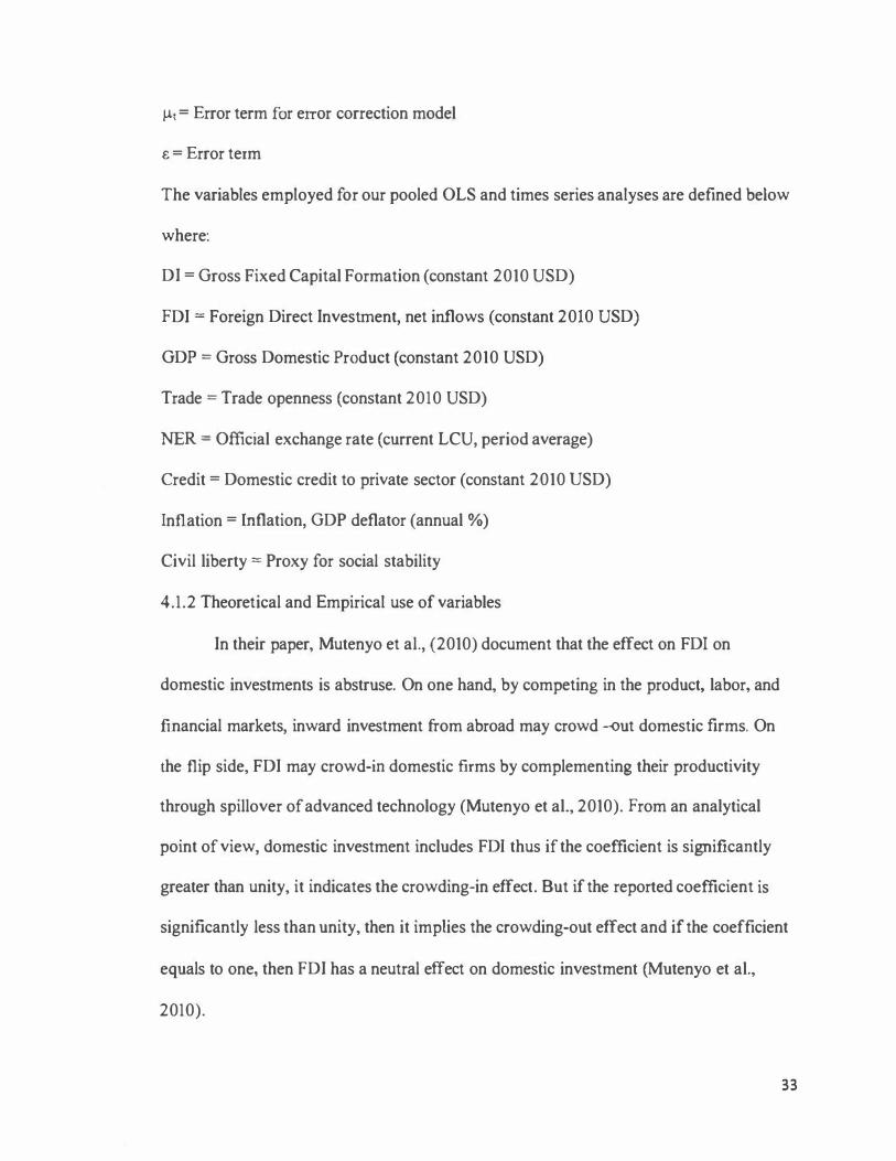
µ1 = Error term for error correction model
s = Error term
The variables employed for our pooled OLS and times series analyses are defined below
where:
DI = Gross Fixed Capital Formation (constant 2010 USD)
FDI = Foreign Direct Investment, net inflows (constant 2010 USD)
GDP = Gross Domestic Product (constant 2010 USD)
Trade = Trade openness (constant 2010 USD)
NER = Official exchange rate (current LCU, period average)
Credit = Domestic credit to private sector (constant 2010 USD)
Inflation = Inflation, GDP deflater (annual %)
Civil liberty = Proxy for social stability
4.1.2 Theoretical and Empirical use of variables
In their paper, Mutenyo et al., (2010) document that the effect on FDI on
domestic investments is abstruse. On one hand, by competing in the product, labor, and
financial markets, inward investment from abroad may crowd -out domestic firms. On
the flip side, FDI may crowd-in domestic firms by complementing their productivity
through spillover of advanced technology (Mutenyo et al., 2010). From an analytical
point of view, domestic investment includes FDI thus if the coefficient is significantly
greater than unity, it indicates the crowding-in effect. But if the reported coefficient is
significantly less than unity, then it implies the crowding-out effect and if the coefficient
equals to one, then FDI has a neutral effect on domestic investment (Mutenyo et al.,
2010).
33

Mutenyo et al., (2010) in their paper accounted that private investment according
to the neoclassical investment theory is assumed to be positively related to the growth of
real GDP (Green and Villanueva, 1 991 ; Fielding 1997; Mutenyo et al., 2010). In the same
light, we postulate that higher income levels will positively affect domestic investment
since an increase in income would lead to higher savings which then causes a spur in the
growth of financing investment. GDP is a predictor variable in the determinant model.
The relevance for GDP growth is that a growing economy will improve the prospects of
market potential. Profit-maximizing investors have high confidence in fast-growing
economies to take advantage of future market opportunities (Li and Resnick, 2003). High
growth economies indicate stable and credible macroeconomic policies which give green
light to domestic investors to invest.
Openness of an economy to the international market makes it more competitive.
As a result, increase in trade openness will mean high level of domestic investment to
meet up with the international demand. The ease of capital movement to and out of the
country and the trade openness of the country affect the domestic investment. Taking it
from the standard point of view, countries with capital control and restrictive trade
policies discourage business, relative to countries with liberal policies. On the other hand,
critics of trade liberalization claim that it can cost jobs because cheaper goods could flood
the domestic market. A very open country allows countries to trade goods without
regulatory barriers or their associated cost. Trade liberalization increases competition
from abroad, which might provide an incentive for greater efficiency and cheaper
production by domestic firms. It might also act as an incentive for an economy to
reallocate resources to industries they may have a competitive advantage in. Citing an
34

example to buttress this point, trade liberalization has encouraged the UK to concentrate
on the service sector rather than the manufacturing. On the cons of trade liberalization,, it
can negatively affect certain businesses within a nation because imported products
increase the competition from foreign producers and may result in less local support for
certain industries. In addendum, trade openness can also pose a threat to developing
nations or economies because free trade introduces stiff competition from more
established economies or nations. According to Asante (2000) restrictive trade regime has
a negative effect on private investment, while trade liberalization affects it positively.
Conversely, Bibi et al., (2012) in his study of Pakistan found that trade openness affects
negatively the domestic investment in Pakistan because trade openness helps in creating
more chances for the outflow of capital out of the economy. In equal vein, Frimpong and
Marbuah (20 10) found that trade liberalization leads to a rise in the foreign competition
of domestic private investment which affect private investment negatively in Ghana.
According to Mutenyo et al., (2010), financial markets in developing economies
are generally underdeveloped. Most domestic firms in these countries rely heavily on
banks for loans or credits. In this vein, credit policies would affect domestic investment
through the stock of credit available that have access to preferential interest rates
(Mutenyo et al., 2010). As our a priori expectations, we hypothesize that availability of
bank credits will have a positive impact on domestic investment. Some past studies
confirm this hypothesis (Gomanee et al., 2005; Ouattara, 2004).
The rate of inflation used as a proxy for the health of the economy is included to
capture the uncertainty of investment. A rise in domestic inflation relative to foreign
inflation with a given level of real exchange rate causes the nominal exchange rate to
35

depreciate adversely hurting investors who rely on imported goods for their business
operations. Macroeconomic instability is manifested by double-digit inflation, large
external deficits, and excessive budget deficits (Benjamin 2012; Demelew, 2014). While
a stable single-digit inflation rate is apparently known to indicate a sign of economic
stability, a high inflation, on the other hand, is perceived as a sign of instability of the
macroeconomic policy. Stated differently, it is recommended that the stability of price
levels is a potent driver for investment and growth. Onyeiwu et al., (2004) states a high
rate of inflation results from irresponsible monetary policy and fiscal policies, including
excessive money supply, budget deficits and a poorly managed exchange rate regime (
Demelew, 2014). On a general note, inflation increases the cost of capital for investors
and this affects profitability adversely and subsequently discourages investment and
economic growth. We hypothesize that inflation which is used as a proxy to measure
macroeconomic uncertainty will be negatively related to domestic investment.
Olson (1996) pointed out that the complex system of political and social
institutions are not given the maximum light in empirics. Mutenyo et al., (2010) argues
that political freedom and civil rights seem to be an important factor for public
investment. Defending their points, they said that benefits of investment spending
generally are not realized in the short-run thus dogmatic policymakers at the helm of
affairs will be inclined to reduce capital spending. In this light, we used civil liberty as a
proxy for social stability. We hypothesize that improved civil liberty in the short -run
will disrupt domestic investment due to higher social instability but this will correct itself
in the long -run.
36

4.2 Data
Gross Fixed Capital Formation (constant 2010 USD): Gross fixed capital
formation (formerly gross domestic fixed investment) includes land improvements
(fences, ditches, drains, and so on); plant, machinery, and equipment purchases; and the
construction of roads, railways, and the like, including schools, offices, hospitals, private
residential dwellings, and commercial and industrial buildings. According to the 1993
SNA, net acquisitions of valuables are also considered capital formation.
Foreign Direct Investment, net inflows (constant 2010 USD): Foreign direct
investment are the net inflows of investment to acquire a lasting management interest ( 10
percent or more of voting stock) in an enterprise operating in an economy other than that
of the investor. It is the sum of equity capital, reinvestment of earnings, other long-term
capital, and short-term capital as shown in the balance of payments. This series shows net
inflows (new investment inflows less disinvestment) in the reporting economy from
foreign investors.
Gross Domestic Product (constant 2010 USD): GDP at purchaser's prices is the
sum of gross value added by all resident producers in the economy plus any product taxes
and minus any subsidies not included in the value of the products. It is calculated without
making deductions for depreciation of fabricated assets or for depletion and degradation
of natural resources. Data are in constant 2010 U.S. dollars. Dollar figures for GDP are
converted from domestic currencies using 2010 official exchange rates. For a few
countries where the official exchange rate does not reflect the rate effectively applied to
actual foreign exchange transactions, an alternative conversion factor is used.
37

Trade openness (constant 2010 USD): Trade is the sum of exports and imports of
goods and services.
Official exchange rate (LCU per USD, period average): Official exchange rate
refers to the exchange rate determined by national authorities or to the rate determined in
the legally sanctioned exchange market. It is calculated as an annual average based on
monthly averages (local currency units relative to the U.S. dollar).
Domestic credit to private sector (constant 2010 USD): Domestic credit to private
sector refers to financial resources provided to the private sector by financial
corporations, such as through loans, purchases of non-equity securities, and trade credits
and other accounts receivable, that establish a claim for repayment. For some countries
these claims include credit to public enterprises. The financial corporations include
monetary authorities and deposit money banks, as well as other financial corporations
where data are available (including corporations that do not accept transferable deposits
but do incur such liabilities as time and savings deposits). Examples of other financial
corporations are finance and leasing companies, money lenders, insurance corporations,
pension funds, and foreign exchange companies.
Inflation, GDP deflator (annual %): Inflation as measured by the annual growth
rate of the GDP implicit deflator shows the rate of price change in the economy as a
whole. The GDP implicit deflator is the ratio of GDP in current local currency to GDP in
constant local currency.
Civil liberties: This rates the freedom status of a country that allow for the
freedoms of expression and belief, associational and organizational rights, rule of law,
and personal autonomy without interference from the state to be measured. The
38

measurement is on a one-to-seven scale with one representing the highest degree of
Freedom and seven the lowest. For easy interpretation, we ordered the scale in an
ascending order where one represents the lowest degree of Freedom and seven the
highest.
4.2. l Sources of data
Data for this investigation purpose came from different sources. A plethora of
parameters was considered to unequivocally figure out the relationship between FDI and
domestic investment. Data from World Development Indicators (WDI), United Nations
Conference on Trade and Development (UNCT AD), and Freedom house index sources
from (www.freedomhouse.org) were used to address the given research question. The
dataset covers the period from 1972 - 201 1 for both Kenya and South Africa.
39

CHAPTER FIVE
DISCUSSION AND POLICY RECOMMENDATION
This chapter will cover descriptive statistics, correlation matrix, discussions of
empirical results, and policy recommendation.
5 . 1 Descriptive Statistics and Correlation Matrix
From Table 5.1 , domestic investment chalked an average of27.4 billion US
dollars with a maximum investment of 87 billion US dollars for both countries. On
average, FDI inflow in the pooled data set is estimated to be around 1 . 1 7 billion US
dollars with a standard deviation of2.89 billion US dollars. This shows there is a
considerable variation in the inflow of FDI in these two countries put together over the
study period. Real GDP was estimated to sit around 1 32 billion US dollars over 40 years
with high variations in around 120 billion US dollars. Trade which contributes a bigger
share to the growth is averaged at 69.5 billion US dollars. Nominal exchange rate was
very volatile with respect to the standard deviation. From the table, inflation and credit
were averaged to be 1 1 .21 % and 133 billion US dollars respectively. The average civil
liberty index for both countries was reported to be approximately 3.75 indicating that
SSA has enjoyed fairly civil freedom over the sample period.
40

T bl 5 1 D a e . escnpt1ve S . . ti K tat1st1cs or enya an d s th Afri OU ca
Variable Obs Mean Std. Dev. Min Max
DI 80 2.74E+l0 2.50E+10 2.04E+09 8.70E+10
FDI 80 l . l 7E+09 2.89E+09 -l .51E+09 l .64E+10
RGDP 80 l .32E+ l l l .20E+l 1 9.67E+09 3.88E+l 1
Trade 80 6.95E+10 6.68E+l0 5.35E+o9 2.70E+l 1
NER 80 22. 12171 27.96175 0.679477 88.81077
Credit 79 1 .33E+ l l l.73E+ l l 1.60E+09 6.0l E+l l
Inflation 80 1 1 .2 1708 6.1 89707 0.933206 41 .98877
Civil Liberty 80 3.725 1 .5 17618 2 6
Table 5.2 shows the correlation between the dependent variable and the
independent variables. It could be seen that all the independent variables were positively
correlated with domestic investment except for nominal exchange rate it was negative.
Additionally, inflation showed a weak correlation with domestic investment.
T bl 5 2 C l . M .
ti K d s th Afr' a e . orre ation atnx or enya an OU ica lnDI InFDI InRGDP In Trade NER
lnDI 1 InFDI 0.6791 1 lnRGDP 0.9899 0.6931 1 In Trade 0.9875 0.7258 0.9942 1 NER -0.5074 -0.2816 -0.47 -0.4653 1 In Credit 0.9784 0.7066 0.9958 0.991 -0.4827 Inflation 0.025 -0.0772 0.003 0.0095 -0.0795 Civil 0.3077 0.5985 0.3885 0.3997 0.0237 Liberty
In Credit Inflation
1 -0.0429 1 0.4458 -0.4029
Civil Liberty
Table 5.3 shows the correlation between the independent variables included in all
the models and does not show any severe collinearity problems.
41
1

T bl 5 3 C l .
M .
f Ind d v .
bl a e orre at1on atnx o epen ent ana es InFDI InRGDP In Trade NER
InFDI 1 InRGDP 0.693 1 1 In Trade 0.7258 0.9942 1 NER -0.28 16 -0.47 -0.4653 1 InCredit 0.7066 0.9958 0.991 -0.4827 Inflation -0.0772 0.003 0.0095 -0.0795 Civil 0.5985 0.3885 0.3997 0.0237 Liberty
5.2 Pooled OLS estimates
In Credit Inflation Civil Liberty
1 -0.0429 1 0.4458 -0.4029
We first run the Pooled Ordinary Least Squares (OLS) to estimate the impact of
FDI on domestic investment in Sub-Saharan Africa using Kenya and South Africa as our
pooled countries. The results are tabulated below with standard errors reported in
parenthesis.
42
1

T bl 5 4 P l d OLS fl K a e . . oo e or en ya & s th Afri 1972 201 1 OU ca, -
Dependent Variable: InDI Variables Model I MODEL II MODEL III MODEL IV InFDI -0.0262674 -0.005401 1 -0.0044584 -0.00 1 1 684
(0.01 5983) (0.012282) (0.01 1782) (0.012) InRGDP 0.6524108*** 1.72625*** 1 . 833983*** 1 .665279* * *
(0. 1 56454) (0. 190465) (0. 187363) (0.2329) In Trade 0.3915381 ** 0.42 18728*** 0.4588474*** 0.4689645***
(0. 17121) (0. 1 32668) (0. 128014) (0.1278) NER -0.0022037*** -0.0038639*** -0.0041563*** -0.0036917***
(0.000772) (0.000619) (0.000604) (0.0007)
In Credit -0.70101 1 1 *** -0.793 13 12)*** -0.6863637*** (0.094735) (0.097639) (0. 1 3 13)
Inflation -0.0065 106** -0.007125*** (0.002531) (0.0026)
Civil Liberty -0.022 1 125 (0.01 83)
CONS - 1 .93383**** - 12.88087*** -14.18467*** -12.78384*** (0.475473) (1.52 1 191) (0. 1 544 1 1 9) (0. 1 .925)
R-SQUARE 0.9848 0.9917 0.9925 0.9927 ADJ R- 0.9839 0.99 1 1 0.9918 0.9919 SQUARE F Statistics 1071 .79 1533.83 1391 .45 1201.7 Prob>F 0 0 0 0 Sample 71 70 70 70 Note: *** Significant at 1 % level; ** Significant at 5% level; * Significant at 10% level
From the table, we had four different models trying to estimate the impact ofFDI
on domestic investment in Sub-Saharan African countries using two countries namely
Kenya and South Africa to make an inference. From Model I, we could infer that a
percentage increase in the log of FD I (InFDI) reduces the log of domestic investment
(InDI) by approximately -0.02 percent holding all else equal. Although, our results
showed a negative relationship between InFDI and InDI, it was insignificant. In other
words, the estimation shows that we do not have enough evidence to prove that FDI
indeed has some impact on domestic investment in SSA countries due to the high P-
value. However, Mutenyo, Asmah, and Kalio (2010) in their investigation of whether
43

FDI crowd-out domestic private investment in Sub-Sahara Africa over the period 1 990 -
2003 found evidence of crowding out effect ofFDI on domestic investment.
Controlling for other observable variables that are independently correlated with
domestic investment, we found out that a one percent change in the log of real GDP
( InRGDP) leads to an approximate 0.65 percentage change in the log of domestic
investment ( InDI) all things being equal. This positive relationship was highly significant
indicating that economic growth stimulate or drives domestic investment in a positive
direction. In addition, the output confirmed our a priori expectations that higher income
levels will positively affect domestic investment since an increase in income would lead
to higher savings which then causes a spur in the growth of financing investment ( Green
and Villanueva, 1991; Fielding 1997; Mutenyo et al., 2010). Trade openness equally
evinced a positive relationship with domestic investment with the coefficient being
significant at 5 percent. The results shows that trade liberalization has positively helped
boost domestic investment over the sample period in SSA. Lastly, there was a negative
relationship between nominal exchange rate and domestic investment. As the local
currency depreciates against the US dollar ( a unit increase in nominal exchange rate), the
log of domestic investment shrinks by 0.2 percent all else equal. The reason could
emanate from the view that, Kenya and South Africa are huge importing countries thus as
the local currency depreciates, importers are faced with high import duties crippling
investment opportunities for them due to the high cost of production.
Moving to Model II, III and IV, lnFDI was consistently having a negative
relationship with lnDI albeit insignificant. In the same vain, the log of real GDP and
Trade openness were both having a significant and positive association with the log of
44

domestic investment. This is to emphasize the importance of the growth of GDP and
trade to the survival of domestic investment. Nominal exchange rate equally registered a
significant negative relationship with the log of domestic investment. This reinforces the
fact that, high depreciation of the local currency in both Kenya and South Africa will
cause a deleterious effect on the activities and operations of domestic investors. In Model
11, we controlled for the availability of resources to domestic investors by including credit
accessibility to domestic investors. It was striking to notice that credit accessibility to the
local investors had a negative relationship with domestic investment. In other words, as
the log of credit increases, the log of domestic investment decreases. The relationship
may be from the fact that as more credit is made available to these domestic investors,
they tend to invest in unproductive ventures. Also, the rate of corruption and bottlenecks
in SSA has been known to be on the high. Due to the high corruption rates in these
countries, increasing credit accessibility may not tend to yield positive results on
domestic investment in the country due to embezzlement of such funds. The level of
inflation in both Model Il1 and IV evinced an adverse impact on domestic investment. As
the level of prices increases, domestic investment tend to reduce. High rate of inflation
indicates an unhealthy economy and thereby discourages investment.
Considering social (and political) stability as a determining factor for domestic
investors in SSA countries, we included Civil Liberty as a proxy for social stability in
Model IV. Even though Civil Liberty might not be the best proxy, that was the best this
paper could utilize over the time period of interest for these countries. This is because we
are dealing with countries where social unrest is recurrent and can be violent to the point
where widespread unrest can ensue and have a nationwide repercussions on economic
45

agents' decision to invest. From Model IV, Civil Liberty is negatively related to domestic
investment. This relationship is not far from the truth because, improved liberties may
breed more social unrest which is possible in a developing country practicing democracy.
These social unrests indicating social instability will definitely impact domestic
investors' decisions thereby reducing domestic investment. It should be emphasized that
this relationship is not significant in the model.
The models reported a very high R-square signifying that the set of independent
variables highly explains the variation of the dependent variable, domestic investment.
Additionally, the probability values for the F-Statistic were all significant indicating that
overall, the model is significant at 1 %.
We subjected our pooled OLS models (I, II, III & IV) to the conventional test for
heteroskedasticity and normality of the residual. This is shown in Table 5.5.
T bl 5 5 n· a e 1asmostics T ti P l d OLS est or oo e ReQTessions Heteroskedasticity (P-Value) Normality( P-Value) MODEL I 0.0003 0.0561 MODEL II 0.5477 0.7841 MODEL III 0.2016 0.842 MODEL IV 0.4171 0.8844 Note: * * * Significant at 1 % level; * * Significant at 5% level; * Significant at 10% level
Using Breusch- Pagan test for heteroskedasticity, Model I failed the test with a p-
value less than 1 % thus rejecting the null hypothesis of constant variance. We concluded
that based on the significant p-value that Model I suffers from non-constant variance.
Utilizing Jarque -Bera test for normality of residuals, Model I barely passed the test for
normality of residuals at 10% significance level. In other words, the residuals for Model I
are not normally distributed at significance level of 1 0%. It is clearly showed on the table
that Model II, III and IV were homoskedastic and having normality of residuals.
46

Table 5.6 Model I adjusted for Heteroskedasticity (Pooled OLS) Dependent Variable: InDI Variables Model I InFDI -0.0262674
(0.0169) InRGDP 0.6524108***
(0. 136) In Trade 0.3915381 ***
(0. 1498) NER -0.0022037***
(0.0006) In Credit Inflation Civil Liberty CONS -1.93383***
(0.3897)
R-SQUARE 0.9848 ADJ R-SQUARE Not Applicable F Stat 1306. 1 1 Prob>F 0 Sample 71 Note: *** Significant at 1 % level; ** Significant at 5% level; * Significant at 10% level
From Table 5.6, Model I is corrected for heteroskedasticity by applying standard
robust errors reported in parenthesis. The corrected model still specifies that the inflow of
FDI has no impact on domestic investment in SSA countries. The log of real GDP and
Trade still maintained significant and had positive relationship with the log of domestic
investment. Accordingly, nominal exchange rate was significant and negatively related to
the log of domestic investment all else equal.
The reported R-square was 0.9848 which means the set of independent variables
jointly explains 98.48 percent of the variation of the logged values of domestic
investment (InDI).
47

5.3 Time series estimates for Kenya
We investigate the impact of FDI on domestic investment in Kenya over 40 years.
Before running our OLS estimation, we check for unit root for all variables used in the
model which is summarized in Table 5.7. Furthermore, we apply the Engle-Granger
cointegration residual test for Models I, II, III and IV as shown in Table 5.8 and the
results show that all the variables are co-integrated for all the models.
T bl 5 7 U .
ti K a e rut root test or enya usmg ADF Constant Constant and trend Constant Constant and trend
1(0) 1(0) I(l) 1(1) Variables Z(t) Z(t) Z(t) Z(t) lnDI -0.21 8 -2.548 -5.905*** -5.858*** InFDI -6.270*** -6.513*** -10.014*** -9.906*** InRGDP -0.576 -1 .692 -3.685*** -3.601 ** In Trade -1 .062 -3.703** -7.002** * -6.894*** NER 0.142 -2.062 -5.241 *** -5.239*** In Credit -0.380 -3.497 -6.864*** -6.763*** Inflation -4.927*** -4.894*** -9.556*** -9.423*** Civil Liberty -1.210 -1 .735 -6.590*** -6.833*** Note: *** Significant at I% level; ** Significant at 5% level; * Significant at 10% level
The results for the test shows that all the variables used were having unit root at
levels except for InFDI and Inflation which were stationary at level. In addition, InTrade
was stationary at level when considering constant and trend. But all variables became
stationary at first difference therefore the variables are integrated to the order of 1 other
written as 1(1).
T bl 5 8 ADF t f R .d 1 ti K a e tes o est ua s or en ya
ADF test statistic Z(t)
MODEL I -3.780***
MODEL II -3.777***
MODEL III -3.852***
MODEL IV -4.019***
Note: *** Significant at 1 % level; ** Significant at 5% level; * Significant at 10% level
48

From Table 5.8, the test statistic values for the cointegration of the five
regressions or models were all significant at 1 0 percent, 5 percent, and 1 percent ,
showing that the residuals are all stationary and that the variables are co-integrated
therefore there is both a long-run and a short-run relationship among the variables. Since
the Engle-Granger two-step estimation procedure was employed and thus requires a two-
step estimation method for dynamic specifications, both the long-run and short-run
models are estimated using OLS estimation.
T bl 5 9 L a e . ong-run R I . hi b e at1ons lP etween FDI d D an Dependent Variable: InDI Variables Model ! MODEL II InFDI 0.001 6641 0.0016565
(0.01333 1 8) (0.0135)
InRGDP 0.8372603*** 0.8313502*** (0.144386) (0.2524)
In Trade 0.3063638** 0.3062318* (0.1491 89) (0. 1 5 14)
NER -0.0030767** -0.0030931 ** (0.001 249) (0.0014)
InCredit 0.0053789 (0.1871)
Inflation
Civil Liberty
CONS -4.827922** -4.803197* (2.1 82527) (2.3754)
. In " K omest1c vestment m en ya
MODEL III MODEL IV 0.0081472 0.0037239 (0.0125) (0.012465)
1.013751 *** 1 .1 28223*** (0.2382) (0.241864) 0.4532656*** 0.4330454*** (0.147) (0.143683) -0.0028038** -0.0030585** (0.0013) (0.001244) -0.2522585 -0.32461 14 (0.1926) (0.19246) -0.006332 1 *** -0.0054897** (0.0022) (0.002221)
0.025 1468 (0.01503)
-6.883913*** -7.553001 *** (2.2797) (2.25573 1)
R-SQUARE 0.946 0.946 0.9567 0.9602 ADJ R- 0.9399 0.9381 0.9488 0.95 1 5 SQUARE F Stat 153.37 1 1 9.2 121 .51 1 10.23 Prob>F 0 0 0 0 Sample 40 40 40 40 Note: *** Significant at 1 % level; ** Significant at 5% level; * Significant at 10% level
49

The principal goal of this paper is to examine the impact of FDI on domestic
investment. The coefficient of InFDI was approximately 0.002 for Model I which
indicates a percentage change in InFDI leads to InDI changing by 0.0016 percent in the
long-run all else equal. And it must be emphasized that the t statistic was statistically not
significant. Stated differently the inflow of FDI in Kenya has no impact on the domestic
investment over the study period. This results is in consonance with Mwega and Ngugi
(2006) work on investigating the factors that constrain improved net inflows ofFDI into
Kenya and whether Kenya responds differently from other countries regarding the
determinants of FDI. Among the issues they analyzed were the magnitudes of net FDI
inflows, their composition and sectoral destination, as well as the economic, political and
other factors that might influence them. The results of the study confirmed FDI over the
period of their study did not play an important role in the Kenyan economy. The same
was the situation in Model II, III and IV where InFDI reported a positive relationship
with InDI but the t statistic were not significant.
The consistent positive relationship between InRGDP and InDI shows that
economic growth is really imperative for domestic investment to thrive in Kenya. This is
because of the highly significant t statistic values of real GDP across the models. For
example in Model I, a percent increase in InRGDP increases InDI by 0.83 percent all else
equal.
Trade openness equally demonstrated a positive relationship with domestic
investment with the t statistic being significant at 5 percent in Model I, III and IV and 1 0
percent in Model I I . The results shows that trade liberalization has positively helped
so

boost domestic investment Kenya. This positive relationship could be explained that the
opportunity to easily import and export strongly influences domestic investment.
Nominal exchange rate was consistently significant and negatively related to
domestic investment in all the regression models. As the Kenyan Shillings depreciates
against the US dollar, domestic investment shrinks by approximately 0.308 percent all
else equal in Model I. This reinforces the fact that, high depreciation of the local currency
in Kenya cause a deleterious effect on the activities and operations of domestic investors
since production cost tends to be on the rise.
In Model II, we controlled for the availability of resource to domestic investors by
including credit accessibility to domestic investors. This variable reported to be positively
related to domestic investment in the long-run. That is, an increase in credit to the private
sector increases domestic investment by 0.005 percent albeit insignificant. It was striking
to notice that credit accessibility to the local investors had a negative relationship with
domestic investment in Model III and IV. This relationship was in accordance with the
relationship that was established in the pooled regression earlier discussed. The
relationship may be from the fact that as more credit is made available to these domestic
investors, they tend to invest in unproductive ventures. Also, the rate of corruption and
bottlenecks in Kenya had been known to be on the high. It should thus be emphasized
that this variable, credit, in the long run does not significantly explain domestic
investment in Kenya.
As aforesaid, Civil liberty was used as a proxy for social stability in Model IV.
From this model, Civil Liberty was positively related to domestic investment in the long
-run. Notwithstanding the insignificance of the coefficient, it makes a whole lot of sense.
51

That is, increased civil liberties become a positive factor as more accountability, checks
and balances and genuine expression of legitimate needs by the population force
decision-makers to address such needs in order to improve their living conditions and
alleviate poverty through high investments and employment in the long -run.
The models reported a very high R- square signifying that the set of independent
variables highly explains the variation of the dependent variable, domestic investment.
Additionally, the probability values for the F-Statistic were all significant indicating that
overall, the model is significant at I percent.
We subjected our time series (I, II, III & IV) to the conventional test for
autocorrelation, heteroskedasticity and normality of the residual. This is shown in Table
5.10.
T bl 5 10 D" " T £ L a e . iagnost1c ests or OnJ run M d 1 £ K o e s or en ya Durbin Watson Heteroskedasticity(P-Values) Normality( P-Value)
MODEL 0.9470042 0.3995 0.6108 I MODEL 0.9445058 0.3975 0.6068 II MODEL 1 .066908 0.5127 0 .6253 III MODEL 1 . 171748 0.4686 0 .7714 IV Note: *** Significant at 1 % level; ** Significant at 5% level; * Significant at 10% level
The Durbin Watson values for the long run models are reported in Table 5.10.
Using Breusch- Pagan test for heteroskedasticity, all the regression models were
homoskedastic due to their high p-values. Thus we fail to reject the null hypothesis of
constant variance. The Jarque-Bera test for normality of residuals all the models came out
to be normal. In other words, the residuals for Model I, II, III and IV are normally
distributed.
52

5.3.1 Estimation of ECM for Kenya
The short -run Models I, II, III, and fV provide information relating to the
adjustments that occur between the different variables to restore the long-run equilibrium
in response to the short-run disturbances of the domestic investment Models I, II, III, and
IV. For these error correction Models, the differenced variables and the lagged error
correction term (EC-1) whose function is to ensure that the short-run deviations in
relation to the long -run relationship are corrected are thus regressed.
T bl 5 1 1 Sh rt f'i K a e . o -run parsnnoruous regressions or en ya Dependent Variable: AlnDl Variables MODEL I MODEL II MODEL III MODEL IV AlnFDI -0.0025102 -0.001 1755 0.001 7065 -0.0002943
(0.007263) (0.00703 1 ) (0.006543) (0.0065 18) AlnRGDP 2.096183*** 1 .940803*** 2.035134*** 1 .922842***
(0.568284) (0.55287) (0.503707) (0.523632) A In Trade 0.32278 19*** 0.2663395** 0.261 1 1 98** 0.2224485**
(0. 1 1 2714) (0.1 1 2548) (0.102492) (0.104725) ANER -0.0045627 -0.003022 -0.0014506 -0.0010752
(0.00275 1 ) (0.002771) (0.00253) (0.002666) A In Credit 0.2632832* 0.070606 0.091826
(0.137047) (0.14006) (0.148954) A Inflation -0.0039039*** -0.00371 1 2***
(0.001258) (0.001288
A Civil (-0.0032038) Liberty (0.022422) EC (-1 ) -0.6550039*** -0.6793519*** -0.6794713*** -0.6833808***
(0.14599) (0.14124) (0.143876) (0.1 53967)
CONS -0.0483316* -0.0577465** -0.0533445** -0.049 1 1 67** (0.025924) (0.025459) (0.23084) (0.023644)
R-SQUARE 0.587 0.6285 0.7017 0.7027 ADJ R- 0.5244 0.5588 0.6343 0.6235 SQUARE F Stat 9.38 9.02 1 0.42 8.87 Prob>F 0 0 0 0 Sample 39 39 39 39 Note: *** Significant at 1 % level; ** Significant at 5% level; * Significant at 10% level
53

From the short -run parsimonious regressions above, we could infer that the
coefficient of change in InFDI was negative and insignificant in Model I, II and IV
confirming to the fact that in the short run, FDI has no impact on domestic investment.
However, in Model III, AlnFDI reported an approximate positive coefficient of 0.002.
That is, a percentage change in AlnFDI leads to a percentage increase in domestic
investment (AlnDI) by 0.002 percent. But the t statistic is not significant meaning FDI
has no impact on domestic investment in Kenya in the short-run.
Real GDP and Trade were both significant and positively related to domestic
investment in the short-run in Model I. This positive relationship of the variables were
consistent in the remaining models and significant in explaining domestic investment.
Nominal exchange rate had a consistent negative relationship with domestic
investment but was not significant in all the models in the short-run. That is to say,
domestic investors in the short -run do not consider the prevailing exchange rate in
making investment decision but definitely one of the critical factors they consider in the
long run.
The error correction term, EC (-1), was highly significant with a probability value
approaching almost zero. The negative coefficient of the error correction term (-
0.6550039) confirms the existence of long -term equilibrium relationship of the model
and also confirms the existence of a cointegration relationship among the variables in
Model I.
Domestic credit to the private sector was positively related to domestic
investment in the short -run. That means, an increase in credit accessibility to the private
sector by one percent increases domestic investment by approximately 0.263 percent in
54

Model II. This positive relationship was significant but was not in Model ill and IV. It
should be noted that, in the short -run, accessibility to credit increases domestic
investment but reduces domestic investment in the long -run. This switch in relationship
may be due to bottlenecks, inefficiency in the financial system coupled with high rate of
corruption in Kenya.
Civil liberty was negative related to domestic investment and insignificant in the
short -run. This is again not far from truth. In the short -run , with their newfound
freedom of belief, associational and organizational rights, rule of law, and personal
autonomy without interference, it indicates that the population engages in more violent
and unrestful actions that have destabilizing effects across society: sustained strikes,
street manifestations, attempted coups as the military sometimes follows suit and get
involved in the whole process. But this negative effect is corrected in the long -run. It
should be noted here that, Civil Liberty as a proxy for social stability in the short -run
was not meaningful in explaining domestic investment.
The error correction terms were all negative and statistically significant indicating
that there is a long -term equilibrium relationship of the models and also confirms the
existence of a cointegration relationship among the variables.
The models reported a very high R-square signifying that the set of independent
variables highly explains the variation of the dependent variable, domestic investment.
Additionally, the probability values for the F-Statistic were all significant indicating that
overall, the model is significant at one percent.
55

T bl 5 12 ff .
T fi Sh fi K a e iagnost1c ests or ort -run pars1momous regressions or en ya Durbin Watson Heteroskedasticity(P-Value) Normality( P-Value)
MODEL l 1 .8171 14 0.5549 0.7401 MODEL II 1.621969 0.4861 0.4006 MODEL III 1 .614098 0.9201 0.744
MODEL lV 1 .666729 0.6224 0.6645 Note: *** Significant at 1 % level; ** Significant at 5% level; * Significant at 10% level
The error correction models above looks very impressive in terms of its quality as
indicated by the results from the diagnostic tests shown in Table 5.12. The Durbin
Watson values shows there is no autocorrelation in all the models. Additionally, the null
hypothesis of normality, and homoscedasticity were accepted.
5 .4 Time series estimates for South Africa
We investigate the impact ofFDl on domestic investment in South Africa over 40
years. Before running our OLS estimation, we check for unit root for all variables used in
the model.
Furthermore, we apply the Engle -Granger cointegration residual test for all models as
shown in Table 5.14 and the results show that all the variables are co-integrated for all
the models.
T bl 5 1 3 U . fi s h Afr. a e rut root test or out 1ca usmg ADF
Constant Constant and trend Constant Constant and trend 1(0) 1(0) I(l) 1(1)
Variables Z(t) Z(t) Z(t) Z(t) InDl -0.657 -0.922 -3.599*** -3.571 * * InFDI -2.795* -3.508**
InRGDP 0.288 -0.995 -4.294 -4.296***
In Trade -0.580 -1 .549 -5.328*** -5.270***
NER -0.736 -2.383 -5.073*** -4.999 ***
In Credit 0 . 177 -2.460 -5.253*** -5.213 ***
Inflation -2.974** -4.857***
Civil - 1 .469 -2.550 -7.121 *** -7.017***
Liberty
56

Note: *** Significant at 1 % level; ** Significant at 5% level; * Significant at 10% level
The results of the test show that all the variables used were having unit root at levels
except for InFDI and Inflation which were stationary at levels. But the non-stationary
variables were stationary after first difference.
Table 5.14 ADF test of Residuals for South Africa ADF test statistic Z(t) MODEL I -3.522*** MODEL II -4.021 *** MODEL III -4.052*** MODEL IV -4.031 *** Note: * * * Significant at 1 % level; * * Significant at 5% level; * Significant at 10% level
From Table 5.14, the P-values for the cointegration of the five regressions or
models were all significant at 10 percent, 5 percent, and 1 percent, it shows that the
residuals are all stationary at levels and that the variables are co-integrated therefore there
is both a long-run and a short-run relationship among the variables. Since the Engle-
Granger two-step estimation procedure was employed and thus requires a two-step
estimation method for dynamic specifications, both the long-run and short-run models are
estimated using OLS estimation.
57

T bl 5 1 5 L a e . ong-run R l . hi b e at1ons Ip Dependent Variable: InDI Variables Model I InFDI -0.0027888
(0.014054) InRGDP -0.0665235
(0.224103) In Trade 1 .084372***
(0. 1 5 1 84) NER -0.081 0691 ***
(0.013737)
In Credit
Inflation
Civil Liberty
CONS -0.9026741 (3.687204)
etween FDI d D an
MODEL II 0.0000468 (0.013931) 0.5335637 (0.45 1 169) 0.9532242*** (0.194673) -0.0653647*** (0.015208)
-0.282 1 154* (0.1 57458)
-6.020859 (4.803065)
. In . S h Afri omest1c vestment m out ca
MODEL III MODEL IV 0.0007345 -0.0005833 (0.014618) (0.01638) 0.5232366 0.520 1 1 98 (0.463279) (0.473546) 0.9562704*** 0.9563818*** (0.199252) (0.203553) -0.0658578*** -0.0667028*** (0.015712) (0.01662)
-0.2710924 -0.270417 (0.169673) (0.173369) 0.0016302 0.00215 12 (0.00805 19) (0.008645)
-0.003487 (0.017805)
-6.145572 -6.052524 (4.94055) (0.017805)
R-SQUARE 0.8609 0.8821 0.8823 0.8825 ADJ R- 0.8395 0.8576 0.8516 0.8452 SQUARE F Stat 40.24 35.92 28.75 23.61 Prob>F 0 0 0 0 Sample 3 1 30 30 30 Note: *** Significant at 1 % level; * * Significant at 5% level; * Significant at 10% level
The regression results on South Africa showed some interesting dynamism. The
coefficient for InFDI in our baseline model (Model I) was -0.0027888. Thus, a
percentage change in InFDI leads to a -0.0028 percentage change in InDI. This negative
relationship or crowding out effect of FDI on domestic investment was not significant.
Trade openness showed a positive relationship with domestic investment with the
t statistic being significant at 1 percent in Model I, II, III and IV. The results shows that
trade liberalization has positively helped boost domestic investment in South Africa just
as in Kenya in the long -run. This positive relationship could be explained that the
opportunity to easily import and export strongly influences domestic investment.
58

Nominal exchange rate was consistently significant and negatively related to
domestic investment in all the regression models. As the South African Rand depreciates
against the US dollar, domestic investment shrinks by 8.1 percent all else equal in Model
I. This reinforces the fact that, high depreciation of the local currency in South Africa
cause a deleterious effect on the activities and operations of domestic investors since
production cost tends to be on the rise in the long -run.
In Model II, we controlled for the availability of resources to domestic investors
by including credit accessibility to domestic investors. This variable reported to be
negatively related to domestic investment in the long run. That is, a percentage change in
Incredit leads to -0.28 percentage change in InDI albeit insignificant. This relationship
was equally evident in both the pooled regression and Model III and IV of Kenya's
equation albeit not significant in the model. The relationship may be from the fact that as
more credit is made available to these domestic investors, they tend to invest in
unproductive ventures. Also, the rate of corruption and bottlenecks in South Africa had
been known to be on the high thus explaining the inverse relationship. In Model III,
InFDI showed a positive coefficient but was still not significant just as in Model II.
Inflation equally was not significant in both Model III and IV. As aforesaid, Civil
liberty was used as a proxy for social stability in Model IV. From this model, Civil
Liberty was negatively related to domestic investment in the long -run. Notwithstanding
the insignificance of the coefficient, improved civil liberties increases social instability
thus decreasing domestic investment. But, this does not explain the variation of the
domestic investment in the model.
59
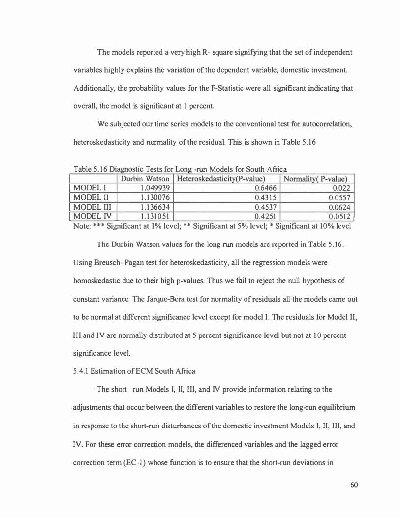
The models reported a very high R- square signifying that the set of independent
variables highly explains the variation of the dependent variable, domestic investment.
Additionally, the probability values for the F-Statistic were all significant indicating that
overall, the model is significant at 1 percent.
We subjected our time series models to the conventional test for autocorrelation,
heteroskedasticity and normality of the residual. This is shown in Table 5.16
T bl 5 16 D . .
T a e . 1agnost1c ests or ong -rurt M d l £ S th Afri o e s or ou ca Durbin Watson Heteroskedasticity(P-val ue) Normality( P-value)
MODEL I 1 .049939 0.6466 0.022 MODEL II 1 . 1 30076 0.43 15 0.0557 MODEL III 1 . 1 36634 0.4537 0.0624 MODEL IV 1 . 1 31051 0.4251 0.0512 Note: * * * Significant at 1 % level; * * Significant at 5% level; * Significant at 10% level
The Durbin Watson values for the long rurt models are reported in Table 5.16.
Using Breusch- Pagan test for heteroskedasticity, all the regression models were
homoskedastic due to their high p-values. Thus we fail to reject the null hypothesis of
constant variance. The Jarque-Bera test for normality of residuals all the models came out
to be normal at different significance level except for model I. The residuals for Model II,
III and IV are normally distributed at 5 percent significance level but not at 1 0 percent
significance level.
5.4.1 Estimation of ECM South Africa
The short -run Models I, II, III, and IV provide information relating to the
adjustments that occur between the different variables to restore the long-run equilibrium
in response to the short-rurt disturbances of the domestic investment Models I, II, III, and
IV. For these error correction models, the differenced variables and the lagged error
correction term (EC-1 ) whose function is to ensure that the short-run deviations in
60

relation to the long -run relationship are corrected are thus regressed and reported in
Table 5.17.
T bl 5 17 Sh ti s th Afri a e . ort -run parsrmoruous regressions or OU ca Dependent Variable: �InDI Variables Model I MODEL II MODEL ill MODEL IV �InFDI -0.0091301 * -0.0089439 -0.009809 -0.0101 143
(0.005275) (0.005651) (0.005943) (0.0062) �InRGDP 0.9161281 0.6319369 0.7561914 (0.7756002)
(0.804748) (0.978436) (1.017257) (1.095) �InTrade 0.259483 0.367295* 0.3445048* 0.3379894
(0.162 1 1 8) (0. 185823) (0.193533) (0.2094) �NER -0.0323637** -0.0290087** -0.0265958* -0.026483 1
(0.012942) (0.01354) (0.015031) (0.0161) �InCredit -0.1874984 -0.1 84708 -0.1901965
(0. 135214) (0. 1 37468) (0. 1438) �Inflation -0.0009463 -0.0010042
(0.003522) (0.0037) �Civil Liberty -0.0029293
(0.0082) EC (-1) -0.6565281 *** -0.6829815*** -0.6906796*** -0.6816063 * **
(0.102972) (0. 1 13222) (0. 1 1 5843) (0.1216)
CONS -0.0005059 0.0170159 0.0137474 0.0 13 1617 (0.019584) (0.023817) (0.024739) (0.0267)
R-SQUARE 0.7634 0.7552 0.7637 0.7575 ADJ R- 0.707 0.6778 0.6717 0.6434 SQUARE F Stat 13.55 9.77 8.31 6.64 Prob>F 0 0 0 0 Sample 27 26 26 26 Note: *** Significant at 1 % level; ** Significant at 5% level; * Significant at 10% level
From the short -run parsimonious regressions above, we could infer that the
coefficient of �InFDI was negative and significant in Model I which is our baseline
model. A percentage change in �InFDI leads to an approximate -0.009 percentage
change in �lnDI all else equal. At 10 percent significance level, we reject the null
hypothesis of FDI not having impact on domestic investment. In other words, we have
61

evidence that FDI indeed displaces domestic investment in South Africa over the study
period .
.6lnRGDP and .6lnTrade were both insignificant and positively related to
domestic investment in our baseline model but nominal exchange rate was highly
significant at 5 percent significance level. That is, the depreciation of the South African
Rand (an increase in NER) reduces domestic investment by 3.2 percent all things being
equal. In Model II, our main independent variable .6InFDI was still having a negative
coefficient but was not significant this time around. Meaning, we do not have enough
evidence to reject the null hypothesis of FDI not having an impact on domestic
investment. But .6lnTrade was significant in Model II. With the positive coefficient, a
unit increase in .6InTrade boost .6InDI by 0.36 percent ceteris paribus. This is to shed
light on the importance of trade openness in positively influencing domestic investors'
decision while holding all the other independent variables constant.
Nominal exchange rate in Model II again confirmed our a priori expectations of
having a negative relationship with domestic investment . That is to say reiterate the fact
that, domestic investors in South Africa definitely consider the prevailing exchange rate
in making investment decision both in the short and long -run.
In Model III and IV, .6lnFDI was still not significant in explaining domestic
investment likewise real GDP, credit accessibility and inflation rate. It should be noted
that trade openness and nominal exchange rate were both significant in Model ill
following the expected sign. Civil liberty introduced in the last model was negative
related to domestic investment and insignificant in the short -run. This is again not far
from truth. In the short-run , with their newfound freedom of belief, associational and
62

organizational rights, rule of law, and personal autonomy without interference, it
indicates that the population engages in more violent and unrestful actions that have
destabilizing effects across society: sustained strikes, street manifestations, attempted
coups as the military sometimes follows suit and get involved in the whole process. It
should be noted here that, Civil Liberty as a proxy for social stability in the short -run
was not meaningful in explaining domestic investment.
The error correction terms, EC (-1) for all the models were highly significant with
a probability value approaching almost zero. The negative coefficient of the error
correction term confirms the existence of long -term equilibrium relationship of the
model and also confirms the existence of a cointegration relationship among the variables
in all the models.
The models reported a very high R-square signifying that the set of independent
variables highly explains the variation of the dependent variable, domestic investment.
Additionally, the probability values for the F-Statistic were all significant indicating that
overall, the model is significant at 1 %.
£ s T able 5.18 Diagnostic Tests or hort -run parslillonious regressions Durbin Watson Heteroskedasticitv(P-val ues) Normality( P-value)
MODEL I 0.9244837 0.9828 0.1902 MODEL II 0.8698506 0.43 17 0.5018 MODEL III 0.865301 1 0.3921 0.5597 MODEL IV 0.8783099 0.3753 0.5534
Note: * * * Significant at 1 % level; * * Significant at 5% level; * Significant at 10% level
The error correction models above looks very impressive in terms of its quality as
indicated by the results from the diagnostic tests shown in Table 5.18. The Durbin
Watson values are reported. Additionally, the null hypothesis of normality, and
63

homoscedasticity were accepted. Thus, all our models are not suffering from
heteroskedasticity and the residuals are normally distributed.
5.5 Policy Recommendation
Our research work showed that FDI was not a significant driver of domestic
investment in the pooled sample but real GDP, trade, exchange rate, inflation, and credit
were strong predictors of investment in SSA. As to recommendations, policymakers in
this region should really put measures in place to foster the growth of the economy.
Economic growth entails a host of factors including improvement in human capital,
infrastructural development among others. A growing economy suggests well-established
infrastructures like roads, electricity, telephone, internet access, airports, vibrant and
working public institutions among others which goes a long way to significantly reduce
the cost of doing business. Thus, decision makers for this region should earmark a
significant portion of their GDP towards investment in the home country. Some countries
like China, Japan, and South Korea just to name a few have adopted similar policies of
boosting their domestic investments and are now enjoying the gains from such policy.
These indicators in place will definitely boost the investment climate in the region.
In South Africa to be particular, we suggest the government introduce a selective
treatment policy regarding the enticement of foreign investors into the country especially
with the sectors already flooded by local investors. If not, this will definitely worsen the
plight of the country by shooting unemployment rate via the displacement of local
businesses. In the effort to attract these foreign investors, there should be strong policies
to safeguard and protect small and growing domestic investments from the market
64

stealing mechanism and open up for more inward foreign investment in sectors where
FDI is having a spillover on domestic investment.
Furthermore, volatility of the exchange rate should be contained. A stable
exchange rate and inflation rate will definitely be a good indicator of a stable economy
and a congenial one for business. In addition, increasing openness to international trade is
associated with significant growth rates. The research is to inform policymakers in Kenya
and South Africa that trade policies have played a huge role in domestic investment. As
such, trade policies that encourage specializations in areas of comparative advantage,
import substitution strategies should be enacted fortified by the stability in the exchange
rate and inflationary rate. Both governments rather should be redirecting it spending
towards economic and social infrastructure that promotes both traditional and
nontraditional exports. The region should also fight corruption and bottlenecks in the
system to give a leeway for credit to positively impact local investment.
65

CHAPTER SIX
CONCLUSION
This theses investigated the impact ofFDI on domestic investment in Kenya and
South Africa during the period of 1972 -201 1 . Using SSA for our preliminary
discussions, the study employed pooled OLS to examine the relationship between FDI
and domestic investment in both Kenya and South Africa. After applying this
econometric technique, the study found that there is no relationship between the inflows
ofFDI and domestic investment during the study period. In other words, the study did not
have enough statistical evidence to prove that FD! has any crowing -out or crowding -in
effect on domestic investment in the SSA region in all four models.
Controlling for other independent variables that strongly predicts domestic
investment in SSA, real GDP and trade openness came out strongly significant and
positive in explaining domestic investment in all the four models. Additionally, nominal
exchange rate and inflation were consistently having a negative impact on domestic
investments in all models. This is to suggest that, high inflationary rate and constant
depreciation of the local currency over the study period showed disinvestment on the part
of local investors. Surprisingly, domestic credit to investors showed a consistently
negative effect on domestic investment in Model II, ill and IV. This relationship could
emanate from the fact that, more credit is made available to these domestic investors,
they tend to invest in unproductive ventures. Civil liberty which was used as a proxy for
social stability was negatively correlated with domestic investment but was insignificant.
Conducting an individual investigation through time series for each country, we
found out that FDI in both the short -run and the long -run had no impact on domestic
66

investment in Kenya. But FDI displayed a crowding -out effect in our baseline model
(Model I) in the short -run period. This is to suggest that South Africa in the attempt of
attracting more FDI to counterbalance the fall in domestic investment was rather hurting
domestic enterprises in the short -run.
Real GDP and trade openness were positively related to domestic investment in
both the short and long -run periods in Kenya. In South Africa, real GDP was an
insignificant determinant of domestic investment in both the short -run and long -run
period whiles trade in the long -run was a positive determinant of domestic investment in
South Africa. Additionally, trade was positive but significant in only Model II and III.
Nominal exchange rate had a negative relationship with domestic investment in
the short -run period in Kenya but this was not significant. However, it was a
determining variable to Kenyan investors in the long -run. A persistent decline in the
value of the Kenyan shillings against the US dollar in the long -run negatively affected
domestic investment. Comparatively, the depreciation of the South African Rand against
the US dollar was negatively related to domestic investment in the short -run. In
opposition to local investors in Kenya, local investors in South Africa do consider the
prevailing exchange rate to be really critical in their decision to invest in the short -run.
But this negative relationship was not significant in the last short -run model. In the long
-run, South Africa shared the same story of Kenya where the persistent decline in the
South African Rand against the US dollar negatively affected domestic investment and
was significant.
Domestic credit accessibility in Kenya was significant and positively related to
domestic investment in the short -run period for Model II. However, the opposite was
67

observed in South Africa where domestic credit was having a negative relationship with
domestic investment albeit insignificant in all the short -run models. In the long -run,
domestic credit was not a significant determinant of domestic investment in Kenya. This
was in consonance to the work of Oshikoya (1994) who found no empirical relationship
between bank credit and private investment for Morocco, Tanzania, and Zimbabwe. On
the other hand, domestic credit evinced a significant and negative relationship with
domestic investment in the long -run period for Model II.
Controlling for macroeconomic stability, high inflation rate was negatively
correlated with domestic investment in Kenya in both the short -run and the long -run.
On a general note, inflation increases the cost of capital and thus negatively affecting the
profit of domestic firms and subsequently discouraging both old and potential investors.
Conversely, this was not a determining factor in South Africa. In addendum, civil liberty
which was used as a proxy for social stability was not a significant determinant of
domestic investment in both countries.
In a nutshell, this theses established that in the pooled sample, FDI was not a
consequential driver for domestic investment. In the time series analyses, FDI had no
impact on domestic investment in Kenya in both the short and long -run period but
exhibited a crowding -out effect on domestic investment in South Africa in the short -
run.
68

References
Acar, S., Eris, B., & Tekce, M. (2012, September). The effect of foreign direct
investment on domestic investment: Evidence from MENA countries. Jn
European Trade Study Group 14th Annual Conference, Leuven, Belgium (pp. 13-
15).
Agosin, M. R., & Machado, R. (2005). Foreign investment in developing countries: does
it crowd in domestic investment?. Oxford Development Studies, 33(2), 149-162.
Ahmed, K. T., Ghani, G. M., Mohamad, N., & Derus, A. M. (2015). Does inward FDI
crowd-out domestic investment? Evidence from Uganda. Procedia-Social and
Behavioral Sciences, 1 72, 419-426.
Ajayi, S.I. (2006). The determinants of Foreign Direct Investment in Africa: A survey of
the evidence. Foreign direct investment in Sub-Saharan Africa: Origins, Targets,
Impact and Potential. Nairobi, Kenya: African Economic research Consortium.
Akinlo, A.E. (2004). Foreign direct investment and growth in Nigeria: An empirical
investigation Journal of Policy Modeling, 26(5), 627 -639.
Al-Sadig, A. (2013). The effects of foreign direct investment on private domestic
investment: evidence from developing countries. Empirical Economics, 44(3),
1267-1275.
Anyanwu, J. C. (2012). Why Does Foreign Direct Investment Go Where It Goes?: New
Evidence From African Countries. Annals of Economics & Finance, 13(2).
Apergis, N., Katrakilidis, C. P., & Tabakis, N. M. (2006). Dynamic linkages between FDI
inflows and domestic investment: a panel cointegration approach. Atlantic
Economic Journal, 34(4), 385-394.
69
Arvanitis, A. (2006). Foreign direct investment in South Africa: why has it been so low?
Retrieved from
https://www.imf.org/extemal/pubs/nft/2006/soafrica/eng/pasoafr/sach5.pdf.
Asiedu, E. (2006). Foreign direct investment in Africa: The role of natural resources,
market size, government policy, institutions and political instability. The World
Economy, 29(1), 63-77.
Bende-Nabende, A. (2002). Foreign direct investment determinants in Sub-Sahara Africa:
A co-integration analysis. Economics Bulletin, 6( 4 ), 1-19.
Benjamin, 0.N. (2012). Foreign direct investment in Sub-Saharan Africa. African
Journal of Economic and Sustainable Development, 1(1), 49 -66.
Bibi, S., Khan, U.A., & Bibi, A. (2012). Determinants of Investment in Pakistan.
Academic Research International, 2(2), pp.517-524.
Blanchard, 0. J., & Gali, J. (2007). The Macroeconomic Effects of Oil Shocks: Why are
the 2000s so different.from the 1970s? (No. wl3368). National Bureau of
Economic Research.
Borensztein, E., De Gregorio, J., & Lee, J. W. (1998). How does foreign direct
investment affect economic growth? 1. Journal of international Economics, 45(1),
1 1 5-135.
Cleeve, E. (2008). How effective are fiscal incentives to attract FDI to Sub-Saharan
Africa? The Journal of Developing Areas, 42(1), 135-153.
Demelew, T. Z. (2014). Foreign Direct Investment Led Growth and Its Determinants in
Sub-Saharan African Countries.
70

Deok-Ki Kirn, D., & Seo, J. S. (2003). Does FDI inflow crowd out domestic investment
in Korea?. Journal of economic studies, 30(6), 605-622.
Diwambuena, J. M., Magwire, A., Klingelhofer, H. E., & Kaggwa, M. (2017). Foreign
Direct Investment and Economic Growth: The Structural Vector Autoregressive
Approach for South Africa. In Development Finance (pp. 1 99-223). Palgrave
Macmillan, Cham.
Dupasquier, C., & Osakwe, P. N. (2006). Foreign direct investment in Africa:
Performance, challenges, and responsibilities. Journal of Asian Economics,
1 7(2), 241-260.
Fielding, D, (1997). "Adjustment Trade Policy and investment Slumps: Evidence from
Africa" Journal of Development Economics, 52, pp.121-37.
Financial Assistance (Incentives), n.d. Financial Assistance (Incentives). (n.d). Accessed
https://www.thedti.gov.za/financial_assistance/financial_incentive, on May 17,
2018
Frimpong, J.M & Marbuah, G. (2010). The Determinant of Private Sector Investment in
Ghana: An ARDL Approach. European Journal of Social Sciences, 15 (2),
pp.250-261
Gaffey. C. (2017, May 3 1 ). What you should know about Kenya's mega-railway, built
with Chinese money. Retrieved June 2, 2018, from
http://www.newsweek.com/kenya-railway-china-madaraka-express-61 83 57.
Gomanee, K., Girma, S. & Morrissey, 0. (2005). Aid and Growth in Sub-Saharan Africa:
Accounting for Transmission Mechanisms Journal of International Development,
17(8), pp. 1055 - I 076.
71

Government of Kenya, (2008). Kenya Vision 2030; A globally competitive and
prosperous nation. Government Printer: Nairobi.
Government of Kenya, (Various Issues). Economic Surveys. Government Printer:
Nairobi.
Green, J. & Villanueva, D. (1 997): "Private Investment in Developing Countries: An
Empirical Analysis" IMF Staff Papers, 38(/), pp.33-58.
Guma, N. (2013). Special Report -SA public sector investment: can it "crowd in"?
Standard bank. Retrieved from
https://m.research.standardbank.com/Research?view=1 67 14535203d9la54c23946
46faled627bf3-1
Harrison, A. E., & McMillan, M. S. (2003). Does direct foreign investment affect
domestic credit constraints?. Journal of international economics, 61(1), 73-100.
Herzer, D. (2012). How does foreign direct investment really affect developing countries'
growth?. Review of International Economics, 20(2), 396-414.
Jeffrey R. (2016). South Africa needs to attract domestic and foreign investment for
economic growth.
Kamaly, A. (2014). Does FDI crowd in or out domestic investment? New evidence from
emerging economies. Modern Economy, 5(04), 391.
Kenya Economy: Population, GDP, Inflation, Business, Trade, FDI, Corruption. (2018).
Retrieved June 2, 2018, from //www.heritage.org/in<lex/country/Kenya
Kenya Investment Authority (2004). "Investment Promotion Act No. 6." Government
Printer.
72

Lautier, M., & Moreaub, F. (2012). Domestic investment and FDI in developing
countries: the missing link. Journal of Economic Development, 37(3), 1 .
Li, Q., & Resnick, A. (2003). Reversal of fortunes: Democratic institutions and foreign
direct investment inflows to developing countries. International organization,
57(1), 175-212.
Li-jun, Y. X. F. R., & Hong-qin, L. I. (2006). An Empirical Study on the Crowding-out
Effects of FD I on Domestic Investment [J]. Journal of International Trade, 9,
013.
Malik, K. (2013). Human Development Report 2013. The Rise of the South: Human
Progress in a Diverse World.
Matsila, N. R. (2014). Estimation of the private investment functions for the South
African economy (Doctoral dissertation, University of Pretoria).
Maxwell J, Fry, (1995). Foreign Direct Investment in Southeast Asia - Differential
Impacts. ASEAN Economic Research Unit Institute of Southeast Asian Studies.
Misun, J., & Tomsik, V. (2002). Foreign direct investment in central europe-does it
crowd in domestic investment?. Prague Economic Papers, 2002(1).
Morris, R., & Aziz, A. (201 1). Ease of doing business and FDI inflow to Sub-Saharan
Africa and Asian countries. Cross Cultural Management: An International
Journal, 18( 4), 400-4 1 1 .
Morrissey, 0. (2012). FDI in Sub-Saharan Africa: Few linkages, fewer spillovers. The
European Journal of Development Research, 2 4(1 ), 26-3 1 .
73

Mugendi, N.C., & Njuru G. S. Foreign direct investment spill over's on domestic firms: a
case of Kenya's domestic firms. Journal of Economics and Development Studies
(Vol.4, pp.45 -60).
Ndikumana, L. (2003). Capital flows, capital account regimes, and foreign exchange rate
regimes in Africa.
Ndikumana, L., & Verick, S. (2008). The linkages between FDI and domestic
investment: Unravelling the developmental impact of foreign investment in SubO
Saharan Africa. Development Policy Review, 26(6), 713-726.
Njeru, J., & Randa, J. (2001). External effects of fiscal deficits in Kenya. African Journal
of Economic Policy, 8(2), 39-54.
Olson, M. (1996). Distinguished lecture on economics in government: big bills left on the
sidewalk: why some nations are rich, and others poor. Journal of economic
perspectives, 10(2), 3-24.
Onyeiwu, S., & Shrestha, H. (2004). Determinants of foreign direct investment in Africa
Journal of Developing Societies, 20(1-2), 89-106.
Oshikoya, T. W. ( 1994). Macroeconomic determinants of domestic private investment in
Africa: An empirical analysis. Economic development and cultural change, 42(3),
573-596.
Ouattara, B. (2004). Modelling the Long Run Determinants of Private Investment in
Senegal. CREDIT Research Paper, 5 (November), available at:
http://:www.nottingharn.ac. uk/economics/research/credit.
74

Ozturk, I. (2007). Foreign direct investment-growth nexus: a review of the recent
literature. International Journal of Applied Econometrics and Quantitative
Studies, 4(2), 79 - 98.
Prasanna, N. (2010). Direct and indirect impact of foreign direct investment (FDI) on
domestic investment (DI) in India. Journal of Economics, 1 (2), 77-83.
Ram, R. & Zhang, K.H. (2002). Foreign Direct Investment and Economic Growth:
Evidence from cross-country data for the 1990s, Economic Development and
Cultural Change, Vol.51 , P 205-2 15
Ramirez, M. (2006). Does Foreign Direct Investment Enhance Private Capital Formation
in Latin America? A Pooled Analysis for the 1981 -2000 Period. The Journal of
Developing Areas, 40(1), 8 1 -97. Retrieved from
http://www.jstor.org/stable/4193017.
Rodrik, D. (1991). Policy uncertainty and private investment in developing
countries. Journal of Development Economics, 36(2), 229-242.
Ronge, E., & Kimuyu, P. (1997). Private investment in Kenya: trends, composition, and
determinants. Institute of Policy Analysis and Research.
SA Reserve Bank, S.A.R (20 13). Quarterly bulletin. South African Reserve Bank
Pretoria, South Africa.
Socrates, M. K. (2012). Determinants of foreign direct investment in Kenya.
South Africa Economy: Population, GDP, Inflation, Business, Trade, FDI, Corruption.
(2018). Retrieved June 2, 2018, from
//www.heritage.org/index/country/southafrica
75

Tang, S., Selvanathan, E. A., & Selvanathan, S. (2008). Foreign direct investment,
domestic investment and economic growth in China: A time series analysis. The
World Economy, 3 1 (10), 1292-1309.
The World Factbook - Central Intelligence Agency. (2018, May). [Government].
Retrieved June 2, 2018, from https://www.cia.gov/library/publications/the-world
factbook/ geos/ke.html
Titarenko, D. (2005). The influence of foreign direct investment on domestic investment
processes in Latvia.
UNCTAD (1999a). World Investment Report: Foreign Direct Investment and the
Challenge of Development. Geneva: United Nations.
UNCT AD (2005). Investment policy review Kenya, New York and Geneva, United
Nations.
United Nations Conference on Trade and Development (1999).
United Nations Conference on Trade and Development (2016).
World Bank, World Development Indicators, 2010, retrieved from
htpp:// data. worldbank.org/topic/poverty.
Ying-Jun, X. U. (2006). The Influence of FDI on Chinese Domestic Investment:
Crowding in or out?[J]. Journal of International Trade, 8, 0 1 5.
76

Appendix
Appendix 1 : Summary statistics for Kenya
Variable Obs Mean Std. Dev. Min Max
DI 40 4.13E+09 l .66E+09 2.04E+09 8.65E+09
FDI 40 l .56E+08 2.58E+08 941961.7 l .47E+09
RGDP 40 2.22E+10 8.72E+09 9.67E+09 4.24E+l0
Trade 40 l .28E+l0 4.87E+09 5.35E+09 2.57E+1 0
NER 40 40.3957 29.83951 7.00 1 1 92 88.81077
Credit 40 5 . 12E+09 2.73E+09 l .60E+09 l .30E+IO
Inflation 40 10.87959 7.634658 0.933206 41 .98877
Civil Liberty 40 4.675 1.095152 3 6
Appendix 2: Pairwise correlation for Kenya
InFDI InRGDP In Trade NER In Credit Inflation Civil
Liberty
InFDI 1
InRGDP 0.2378 1
In Trade 0.3001 0.96 1
NER 0.2655 0.9083 0.9009 1
In Credit 0.2469 0.9862 0.9531 0.9255 1
Inflation 0.2054 -0.018 0.0725 -0.0302 -0.083 1
Civil 0.2567 0.297 0.3 174 0.3819 0.36 -0.2704 1
Liberty
77

Appendix 3 : Pair wise correlation for Kenya (with dependent variable)
InDI InFDI InRGDP In Trade NER In Credit Inflation Civil
Liberty
lnDI 1
InFDI 0.2448 1
InRGDP 0.9658 0.2378 1
In Trade 0.9446 0.3001 0.96 1
NER 0.8445 0.2655 0.9083 0.9009 1
In Credit 0.9475 0.2469 0.9862 0.9531 0.9255 1
Inflation -0.0707 0.2054 -0.018 0.0725 -0.0302 -0.083 1
Civil 0.3396 0.2567 0.297 0.3 1 74 0.3819 0.36 -0.2704 1
Liberty
78

Appendix 4: Summary statistics for South Africa
Variable Obs Mean Std. Dev. Min Max
DI 40 5.07E+l0 l .22E+l0 3.45E+10 8.70E+l0
FDI 40 2.19E+09 3.84E+o9 -l .5 1E+09 l .64E+l0
RGDP 40 2.41E+l 1 6.70E+l0 l .46E+l l 3.88E+l 1
Trade 40 1 .26E+l l 4.90E+10 6.83E+l 0 2.70E+l l
NER 40 3.847723 2.892791 0.679477 1 0.54075
Credit 39 2.56E+l 1 l .57E+l l 9.59E+IO 5.74E+l l
Inflation 40 1 1 .55458 4.368716 5.449048 24.87883
Civil Liberty 40 3.875 1 .771389 2 6
Appendix 5 : Pairwise correlation for South Africa
InFDI InRGDP In Trade NER In Credit Inflation Civil
Liberty
InFDI 1
InRGDP 0.5681 1
In Trade 0.667 0.9169 1
NER 0.624 0.8995 0.83 1 1 1
In Credit 0.5578 0.9656 0.8445 0.9278 1
Inflation -0.5648 -0.6328 -0.5776 -0.6608 -0.714 I
Civil -0.7292 -0.7264 -0.7732 -0.778 -0.75 19 0.6822 1
Liberty
79

Appendix 6: Pair wise correlation for South Africa (with dependent variable)
InDI InFDI InRGDP In Trade NER In Credit Inflation Civil
Liberty
InDI 1
InFDI 0.43 1 8 1
InRGDP 0.5473 0.5681 1
In Trade 0.7295 0.667 0.9169 1
NER 0.3132 0.624 0.8995 0.83 1 1 1
In Credit 0.382 0.5578 0.9656 0.8445 0.9278 1
Inflation -0.2736 -0.5648 -0.6328 -0.5776 -0.6608 -0.714 1
Civil -0.4039 -0.7292 -0.7264 -0.7732 -0.778 -0.75 1 9 0.6822 1
Liberty
80
Recommended