INVESTIGATION ON THE ANALYTICAL FORM OF THE
TRANSITION MATRIX IN INERTIAL GEODESY
VOON CHOONG WONGKLAUS-PETER SCHWARZ
December 1979
TECHNICAL REPORT NO. 58

PREFACE
In order to make our extensive series of technical reports more readily available, we have scanned the old master copies and produced electronic versions in Portable Document Format. The quality of the images varies depending on the quality of the originals. The images have not been converted to searchable text.
INVESTIGATION ON THE ANALYTICAL FORM OF THE TRANSITION
MATRIX IN INERTIAL GEODESY
Voon Choong Wong And
Klaus-Peter Schwarz
Department of Surveying Engineering University of New Brunswick
P.O. Box 4400 Fredericton, N.B.
Canada E3B 5A3
December 1979
ABSTRACT
The error behaviour of inertial survey systems can best
be described by a system of differential equations. Its solution
in analytical form, by way of a transition matrix, is discussed
in this report.
After a review of the methods available to solve systems
of differential equations, the dynamics matrix of the local-level
system operating in three dimensions is treated in detail. Two
methods are used to derive the analytical form of the transition
matrix: the inverse Laplace transform technique and the series
expansion of the matrix eA~onential. Analytical and numerical compari
sons show that the two derived solutions are not completely equiva
lent but agree very well for time intervals up to 1000 seconds.
For large time spans the inverse Laplace transform solution is more
accurate. The report concludes with a brief discussion of the
effects which the ~ariation of certain parameters has on the
error behaviour.

ACKNOWLEDGEMENTS
This research has been funded by a contract with the
Department of Energy, Mines and Resources and by a research grant
from the National Sciences and Engineering Research Council. The
support is gratefully acknowledged.
TABLE OF CONTENTS
Abstract •••. i
Acknowledgements • ii
1. Introduction 1
2. Solution of Systems of Differential Equa~ions 3
3. Dynamics Matrix 11
3.1 Notation . . • . 11 3.2 Description of the Dynamics Matrix
4. Inverse Laplace Transform Solution ...
4.1 Matrix Inversion by Partitioning Method 4.2 Inverse Laplace Transform Technique . 4. 3 Final Expressions .• . . . • 4.4 Discussion of the Solution
5. Series Solution
5.1 Dasic Technique 5.2 Final Expressions 5.3 Discussion of the Solution
6. Tests and Numerical Results
16
16 18 20 31
33
34 35 43
45
6.1 The Numerical Method 45 6.2 Testing the Inverse Laplace Transform Solution 47 6.3 Testing the Series Solution 49
7. Conclusions. 51
Appendix I • 53
References 58
iv
1. INTRODUCTION
During the last four years inertial survey systems have been
routinely used to establish second-order control and a recent analysis
of extensive test data indicates that first order accuracy may be
achievable (Schwarz, 1979a)". Considering the amount of information
generated by these systems, the integration of this new data type into
existing control is a task of growing importance. Its solution requires
error propagation models ,.,hich take into account the time dependence of
all quantities involved. Thus, the basic mathematical model is a
system of differential equations.
The solution of such systems is usually done today by numerical
integration procedures. The methods are well developed mathematically
and excellent program packages have become available, in recent years.
A review of the state of the art is given in Lambert (1977).
The advantage of this approach is that it is almost universally
applicable, i.e. inhomogeneo~s and nonlinear systems can be treated as
well as the homogeneous case. However, it is very time consuming
computerwise and it does not allow general statements about the stability
of the system and its characteristical features. Thus, analytical
solutions, besides requiring less computer time, can be of great value
to study the general behaviour of a specific system. Generally, such
1

2
solutions can only be obtained for a more restricted class of problems
and even then the amount of formal manipula~ions can be exasperating.
It vas felt, however, that this effort would be well spent for the
study of the error propagation in inertial survey systems. The
following report documents how far this attempt has been successful.
It should be noted at this point that the accuracy of the
final coordinates produced by an inertial survey system is a mixture
of continuous error propagation through a system of differential equations
and update procedures at discrete instants in time which basically are
discontinuous. Here, only the first part is treated. Its solution
sets the scene for the filtering and smoothing procedures which are
used when discrete control measurements become available. The application
of such methods to the error propagation in inertial positioning has
been treated in Schwarz (1979b).
The report has been organized in such a way that a brief
review on the solution of systems of differential equations is given
first. Then~ the system of error equations used in inertial geodesy
is described. Its solution is obtained in two ways, by using the
inverse Laplace transform and by a series expansion of the matrix
exponential. Comparison of results and some numerical studies conclude
the report.
2. SOLUTION OF SYSTEMS OF DIFFERENTIAL EQUATIONS
The inhomogeneous linear system of vector differential equations
x(t) = F(t) x(t) + G(t) u(t) (2-1)
with initial conditions
~(o) = ~
is used as a model for the errors in an inertial survey system. In
this equation vectors are denoted by an arrow and matrices by capital
-+ let~ers. Let us first discuss the homogeneous case u(t) = 0
:ic(t) = F(t) x(t)
with
~(0) = -;
(2-2)
It describes a physical system whose state at any time t is completely
. -+T . T defined by the N functi.ons xi (t) contained ~n x = {x1 , x2 .•. ~}
and whose rate of change at a given time tk depends only on the values
of the functions ~ ( t) at tk. This means that in a: formal way the
solution can be written as
where ~(t, t ) is as yet undetermined. 0
(2-3)
-+ We will call x(t) the state
vector, F(t) the dynamics matrix, and ~(t, t ) the transition matrix. 0
3

4
These names are often used in optimal estimation literature. 4>(t, t ) is 0
-+ a square matrix which in general is nonsymmetric. The vector c •
-+ represents the initial state of the system. If the elements of c
are such that equation (2-2) beco~s zero, we speak of an equilibrium
state. The behaviour of the system in the neighbourhood of such
equilibrium states is of special interest because it determines the
stability of the system. A system is called stable if after perturb-
ations it returns to the equilibrium state; otherwise, we speak of an
unstable system.
In our case the functions x.(t) describes the error charac~
teristics of an inertial survey system. It is obvious that in such a
case equation (2-2) can only be an approximation. It is dependent on
the current knowledge of the error sources and on the requirement that
they can be modelled in the form (2-2). Errors of this type are e.g.
the position, velocity and misalignment errors at the start of the
measurement, gyro drifts and accelerometer biases. If any of these
error sources produce an unbounded error growth, we have an unstable
system. It is well-known (see e.g. Britting, 1971) that this is the
case for the general inertial navigation problem in three dimensions
when no outside information is provided for the altitude channel. The
formulation of the dynamics matrix has therefore been done in such a
way as to exclude this instability.
So far only the homogeneous system has been discussed. The
solution of the more"general system (2-1) can be written in the form
-+ x(t) = 4>(t, t )
0
t -+ c + J
t 0
4>(t, t ) 4>-1 (s, t ) G(s) ~(s) ds 0 0
(2-4)
5
where s is a time variable. A comparison with equation (2-3) shows
that the solution obtained from the homogeneous system is changed by
adding an integral containing the transition matrix and the functions
-+-G(t) • u(t). Since the homogeneous equation describes the unforced
motion of the system, the functions u .. {t)are often called the forcing 1.
functions. They can be either deterministic or random. In the first
case, equation (2-1) is said to define a control problem, in the second
an estimation problem. A combination of both types of problems is
obviously possible. In the applications discussed here the gravity
vector can be considered as a control function while acceler-
ometer noise represents a random forcing function.
In order to obtain a solution of type (2-3) or (2-4) the
transition matrix must be determined. The remainder of this section
will therefore discuss methods to obtain ~(t, t ) in analytical form. 0
The inhomogeneous part of the solution (2-4) will not be treated in
detail. In the problems discussed in this report, the forcing functions
are always considered as random functions with mean zero, and are
therefore handled as part of the optimal estimation procedure.
Equation (2-2) has a unique solution if F(t) is continuous
fort > 0. This solution can be written in the form (2-3) where ~(t, t ) 0
is the unique matrix satisfying the matrix differential equation
~(t, t ) = F(t) t(t, t ) 0 0
with initial conditions
t(t , t ) = I 0 0
(2-5)

6
Among the continuous matrices those with constant coefficients represent
the simplest case. For such a matrix the solution of (2-2) can be
formally written as a matrix exponential
~( ) F(t-t ) ~ x t = e o c (2-6)
Comparison with equation (2-3) results in
"'( t .) = eF(t-to) .'i' t.
0 (2-7)
The matrix exponential can be expanded into an infinite series
F(t-t ) 00 (t-t )i Fi 1:
0 ( 2-8) e o = i=O • I 1.
which in conjunction with equation (2-7) gives the first method to
compute an analytical form of the transition matrix. Using the Cayley-
Hamilton theorem the infinite series expansion can be replaced by a
finite series of order N where N is the rank of F. A discussion of
this case and its usefulness in applications is given in Bierman (1971).
The meaning of the formal solutien (2-6) becomes clearer
when considering the special case F = AI
~(t) AI(t-t ) x = e o -+ d (2-9)
-+ where A is an unknown scalar and d an unr~own vector. When this solution
is introduced into equation (2-2), we obtain fort • 0 0
and thus
(F - U) d = 0 (2-11)
~
If d is not a zero vector, equation (2-2) will only have a solution if
IF- nl = o (2-12)
This equation represents a standard eigenvalue problem where A is the ~
eigenvalue and d the eigenvector. If all A· are distinct then we can 1
transform equation (2-9) into
~
x(t) = N E
i=l e
A. t 1 +
d. 1
(2-12)
where N is again the rank of F. This equation shows that a second method
to obtain an analytical solution is by way of the eigenvalue problem.
If instead of the special case leading to equation (2-9), a full matrix
F with distinct eigenvalues has to be treated, the canonical matrix A
can always be obtained by the transformation
T-l F T = A (2-13)
~here A is the diagonal matrix of eigenvalues and the columns of T are
the eigenvectors. The transition matrix is then of the simple form
~(t, t ) =TeAt T-l 0
At where e can be written as a diagonal matrix of the form
Alt e
A2t 0
e
At e =
0
(2-14)
(2-15)
In case of multiple eigenvalues the situation is more complicated and
reference is made·to textbooks as Gantmacher (1959) and Hochstadt
(1975).
8
A third way to arrive at an analytical form for t(t, t ) is 0
-1 by use of the inverse Laplace transform L • Again it is only appli-
cable to differential equations with constant coefficients. The Laplace
transform L of a function x(t ) is defined as
y(s) = L x(t)
.., = f e -S.t x( t) dt
0
and equivalently for the vector ~(t) of functions xi(t)
;.(s) = L ~(t)
co
= f e-st ~(t) dt 0
-+ where the operation (2-16) is performed on each element of x(t).
(2-16)
(2-17)
The Laplace transform of ~(t) can be found by integrating by parts
(X)
-st -+ -+ ~ f e x( t) dt = s y( s) - x( o) (2-18) 0
Using equations (2-17) and (2-18) the homogeneous equation (2-2) can
be transformed to
or
s-;<s) --+ c =
-+ F y( s)
(si - F) Y<s) -+ = c
(2-19)
(2-20)
Thus, the system of differential equations bas been converted into a
system of algebraic equations. If the inverse of (si -F) exists we
9
have
y(s) = (si - F)g ~ (2-21)
where the index g denotes some suitably defined generalized inverse.
For the Cayley inverse, which is the only one considered hereafter,
equation (2-21) reads
;(s) = (si - F)-l ~ (2-22)
~ -1 Once y(s) has been found the inverse Laplace transform L can be
applied to obtain ~(t)
x(t)
1 = --2trj
a +iw 0 + st f y( s) e ds
a -iw 0
(2-23)
where a0 > a1 and a1 is some allowable region of convergence. Thus, an
i(t) must be found whose transform is y(s). Usually the individual
function y.(s) can be brought into a form which is listed in one of ~
the extensive tables of Laplace transforms. By using equation (2-3),
(2-22) and (2-23) we obtain
which is the desired expression for the transition matrix. Applications
of this technique will be given in chapter 4.
So far only a matrix F with constant coefficients has been
treated. Homogeneous equations with variable coefficients are not
so tractable. In general, it is not possible to derive closed form
solutions. In certain cases, series solutions can be obtained. This

10
applies for instance to systems where F can be expanded into a series
with analytic coefficients. But usually the increase in complexity
is considerable. In many cases the solution from a constant coefficient
matrix represents a good first approximation and is sufficient for
applications. When modelling errors of an inertial system, a constant
F-matrix corresponds to a system without vehicle accelerations. Such
a system reflects all the long term error frequencies. If necessary, the
neglected accelerations can be modelled in a Taylor expansion about the
first approximation as discussed by Lyon (1977) for the two-dimensional
inertial navigation problem. This report treats only the case of
constant coefficients.

3. DYNAMICS !•1ATRIX
3.1 Notation
A number of symbols have been introduced in the last chapter.
To simplify the reference they are listed below together with some.
notations used later on.
(.)-first derivative with respect to time
( )-1- inverse
F - dynamics matrix
~ - transition matrix
R - distance from earth centre to platform
~ - geodetic latitude
X - geodetic longitude
h - height above the reference ellipsoid
g - gravity
~ - Schuler frequence (lg/R)
i - celestial longitude rate (i = ~ + w. ) ~e
wie- earth rate (7.202115 x 10⁻⁵ rad/s)
E - attitude errors
o - coordinate and velocity errors
K1 , K2 - damping loop gains
t - time
11

3.2 DescriPtion of the Pynamics Matrix
It has been mentioned in section 2 that the dynamics matrix
F should model all time dependent errors of the inertial survey system.
As equation (2-3) shows they can be presented as modulations of the
-+ error vector c at the initial point. Britting [1971] has proposed to
formulate a unified error theory by using a nine state vector of three
initial errors for position, velocity and attitude. This approach is
followed here. The much larger state vectors used in the Kalman
filters of inertial survey systems are obtained by splitting the above
errors into physically meaningful components. Thus, the attitude errors
may consists of a misalignment and drift part, t3e velocity errors of
an accelerometer bias and a scale factor. The separation of different
components is in general done by a priori weighting and belongs there-
fore to the estimation part of the problem. A thorough treatment of this
matter would have to include the observability conditions of the
dynamic system as discussed for instance in Fossard [1977] and KortUm
[1974].
The nine state error vector considered in our investigation
is given by
(3-1)
where e:N, e:E, e:D are the attitude errors, cScp, cS:>.., and cSh are the latitude,
longitude, and height errors, and cScj>, cS:>.., and cSh are velocity errors
in latitude, longitude and height.
/1'.,

13
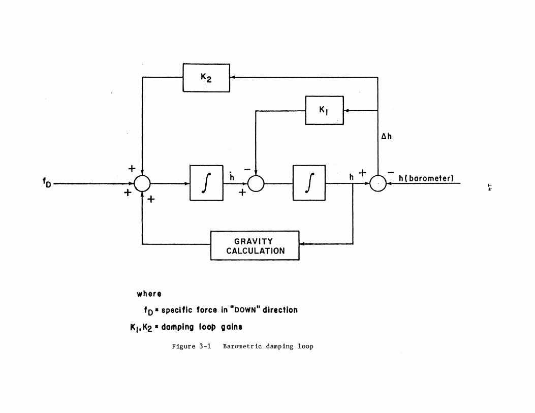
The dynamics matrix F associated with the state vector may
be derived from the specific force equations and the misorientation
error equation given e.g. in Britting [1971] and Adam [1979]. The F
matrix for a local level system that employs a barometric damping
second-order loop (as shown in Figure 3-1) can be found in Schmidt
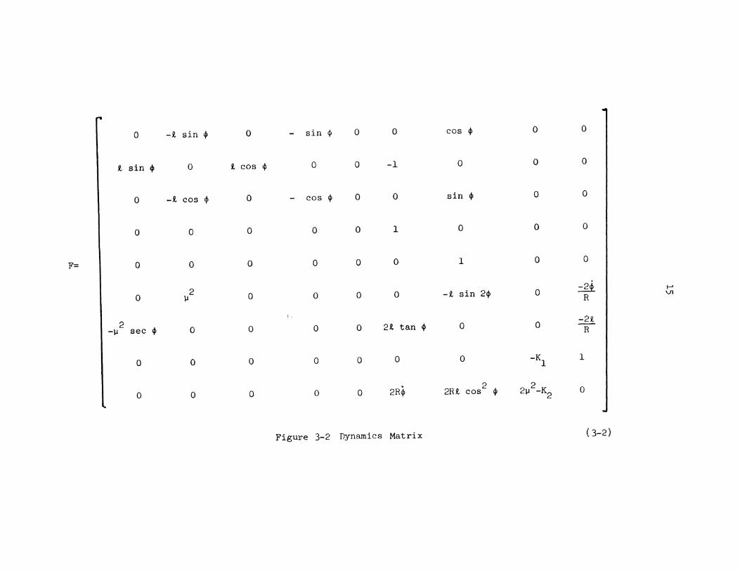
[1978]. By neglecting the time dependent elements and the products
of velocities, the dynamics matrix can be reduced to the form shown
in Figure 3~2. In the aircraft mode, such a system can utilze the
height difference information from the altimeter to dampen the
exponential growth of errors in the height channel and its effect
on the horizontal channels. In theterrestialmode no altimeter data
are available, but the errors are controlled by the information
obtained at every zero velocity update (ZUPT). Thus, the gain
factors K1 and K2 , although derived from a different set of measure
ments, can formally be used in exactly the same way in the F-matrix.
The final expression for the system of differential equation is
given by the matrix in Figure ( 3-2) and the state vector-(~-1).
to
K2 !
-. J
. h
. + +
GRAVITY CALCULATION
-------
where
fo • specific force in "DOWN" direction
K1, K2 • damping lool» gaIns
J
Figure 3-1 Barometric damping loop
Kl
h + .... "'"
0 -R. sin ~ 0 - sin 4> 0 0 cos ~ 0 0
R. sin ~ 0 R, cos ~ 0 0 -1 0 0 0
0 -R. cos ~ 0 - cos 4> 0 0 sin ~ 0 0
0 0 0 0 0 1 0 0 0
F= I 0 0 0 0 0 0 1 0 0
0 2 0 0 0 0 -R. sin 2~ 0
-2t I ......
lJ R \.n
2 sec ~ 0 2R. tan ~ 0 0
-2R. -lJ 0 0 0 R
0 0 0 0 0 0 0 -K 1
1
0 0 0 0 2Rij> 2 2 0 0 2RR. cos ~ 2lJ -K2
Figu'lie 3-2 Dynamics Matrix ( 3-2)

4. INVERSE LAPLACE TRANSFOR.l.! SOLUTION
The inverse Laplace tran~form is one of the techniques
used in solving for th~ transition matrix ~(t) of the system of
differential equations described in the last chapter. Here as in
the following t = 0 has been assumed. The purpose of this chapter 0
is to show how the matrix is derived and to list its fi::1al form.
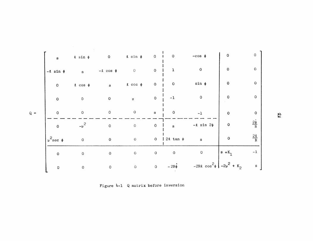
B.r.substituting the dynamics matrix F into equation (2-24),
the system of differential equation may be rewritten in the form shown
in ¥igure 4-1. The most difficult task in deriving the transition
matrix using the inverse Laplace transform is the inversion of the
matrix.
Q = (s:r - F) (4-1)
4.1 Matrix Inversion by Partitionin~ Method
The matrix partitioning method for inverting a matrix
described by Faddeev and Faddeeva [1963] can be used for solving
this problem.
To apply the method, the matrix Q in Figti.Te 4-:l·may be
parti tione·d as follows :
I ---~--- (4-2)
16

17
and the inverse is given as
32 I ' 01 I Ll
-1 I Q = 12 -..- _, ______ (4-3}
where
N. = (Di - CiAi-~i) 1
(4-4)
L. = -A.-~.N. 1 1 1 1 (4-5)
M. N.C.A. -1 = -1 1 1 1 (4-6)
and ~1 -~ -1 0. = A. +A. .N.C.A
1 1 1 1 1 1 ( 4-7)
In this case, the_ method has to be applied twice for inverting
the whole matrix in Figure 4-1. First, the 7 x 7 portion on the top
left hand corner is inver..ted and the partitioning is done as indicated
by the dotted lines. The whole matrix is then partitioned and inverted
according to the solid lines using the inverted 7 x 7 portion as the
-1 new A2 • The inverted top left hand 7 x 7 portion of Figure 4-1 is
shown in Appendix I and the N2-matrix which was derived from standard
co-factor techniques is
s 1
(s-a}{ s-b) (s-a) ( s-b)
N2 = (4-8) 2 (21l -K2 ) s + ~
(s-a)(s-b) (s-a) (~-b)
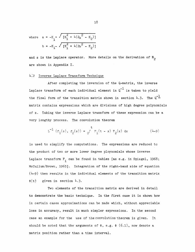
18
wher·e a = -K + I r~ + 1
b = -K1- I [K2 + 1
and s is the Laplace operator. More details on the derivation of N2
are shown in Appendix I.
4:2 Inverse Laplace Transform Technique
After completing the inversion of the Q-matrix, the inverse
Laplace transform of each individual element in Q-l is taken to yield
the final form of the transition matrix shown in section 4.3. -1 The Q-
matrix contains expressions which are divisions of high degree polynomials
of s. Taking the inverse Laplace transform of these expression can be a
very lengthy process. The convolution theorem
t
0J F1(t- x) F2(x) dx (4-9)
is used to simplify the computations. The expressions are reduced to
the product of two or more lower degree ploynomials whose inverse
Laplace transform F. can be found in tables [as e.g. in Spiegel, 1968; l.
McCullum/Brown, 1965]. Integration of the right-hand side of equation
(4-9) then results in the individual elements of the transition matrix
~(t·) given in section 4.3.
Two elements of the transition matrix are derived in detail
to demonstrate the basic technique. In the first case it is shown how
in certain cases approximations can be made which, without appreciable
loss in accuracy, result in much simpler expressions. In the second
case an example for the use of the convolutd.on theorem is given. It
·should be noted that the arguments of~. e.g. ~ (6.1), now denote a
matrix position rather than a time interval.

19
The element ~(6, 1) of the transition matrix is given as
~(6, 1)
Taking the inverse Laplace transform of (4-10), we get
~( 6 , l) = u2 ~ sin p(cos tt-cos ut) + tu2 t sin p ,2 + t2 .. .u
and using the assumption that
1J2 » R.2
(4-11) may be reduced to
~(6, 1) = R. sin ~(cos tt - cos ut + ut sin ut)
(4-10)
(4-11)
( 4-12)
Another more involved element ~(6, 8) is given as
~(6, 8) -1 2 5~ = L { -2(2u-K2 )( 2 2 ~---(s +1J )(s-a )(s -b)
Using the convolution theorem, equation (4-13) may be reduced to
t ( a(t-r) b(t-r)) cos l.:f ~(6, 8) = -2(2u-K2 )[~ f e -e df 0 (a-- b)
- t 2 sin 2~ t r(aea(t-r)_bea(t-r)) sin uf
! df] . ( 4-14) 0 2u (a - b)
which when integrated yields the final form·

20
[~ (u sin J..lt - a(cos )Jt-eat)
( a 2 +)J 2 ) ( a-b )
u sin J..lt - b(cos J..lt - ebt)
( b 2 +)J 2 ) ( a-b )
+ R. 2 sin cp
21J (a-b)
a (t(a sin \.It- \.!COS \.It)
(a2 + \.12)
b (t (b sin \.It - ll cos llt)
(b2 + \.12)
( (b2_, 2) ( bt) .. sin \.It + 2b\.l cos llt-e ) ] (b2 + \.12)
( 4-15)
In the first example, the final form of the element (6, 1)
can be simplified considerably if the assumption \.1 2 >> t 2 holds. The
accuracy.lost, numerically, is less than 1% of the value computed
from equations (4-21). The last example shows how the convolution
theorem can be applied to find the inverse Laplace transform of an
expression.
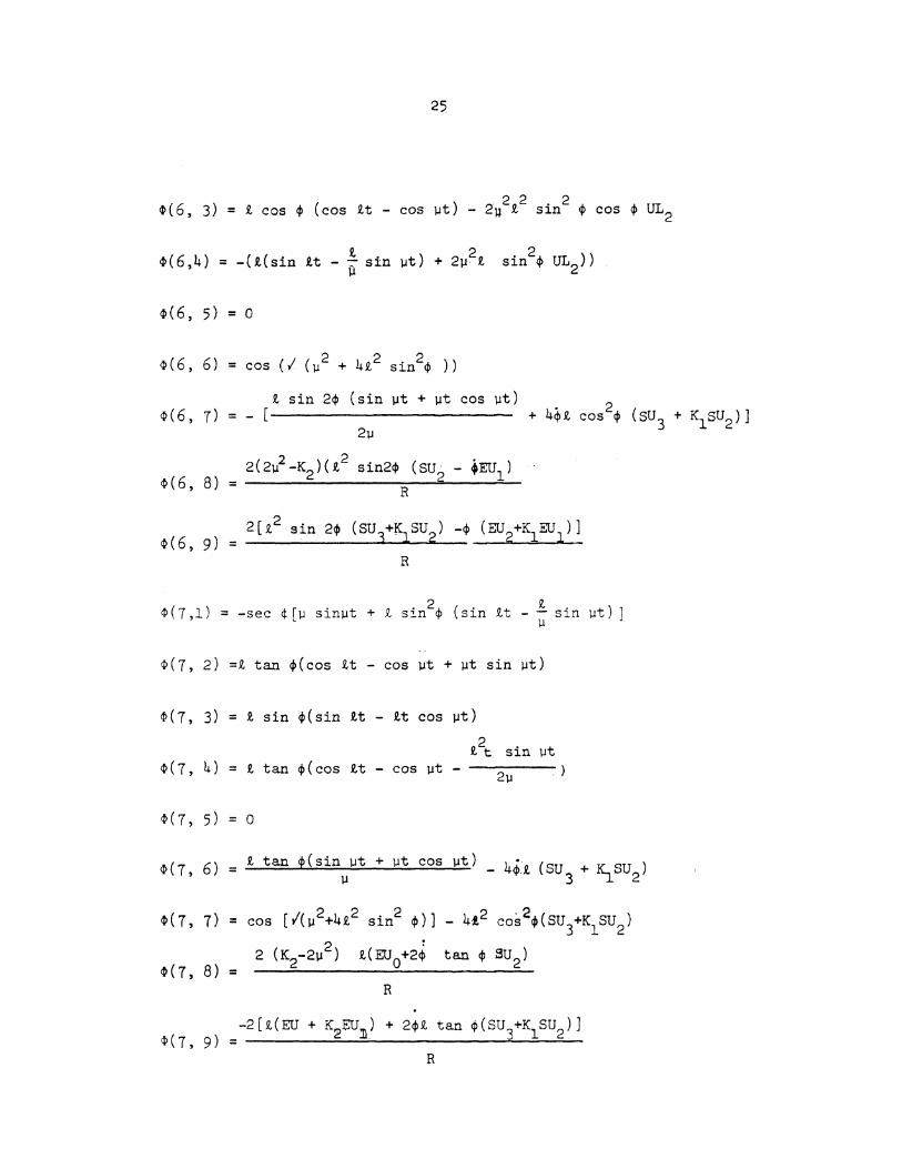
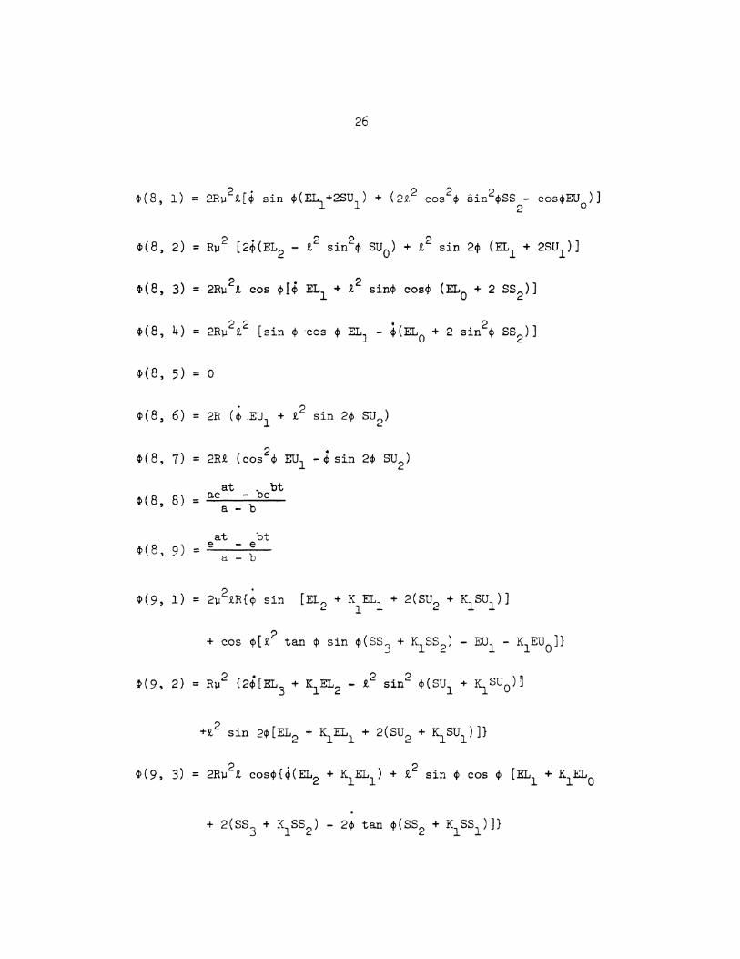
4.3 Final Expressions
Figure 4-1 shows the matrix Q as defined by equation (4-1).
The elements of the transition matrix obtained by forming
~(t) = L-l {Q-l (s)}
are listed below.
s R. sin ~ 0 R. sin ~ 0 I 0 -cos ~ 0 0
I I
-R. sin f s -R. cos ~ 0 0 I 1 0 0 0
I I
0 R. cos ~ s R. cos ~ 0 I 0 sin ~ 0 0
I
0 0 I
-1 0 0 0 s 0 . 0
Q = I 0 0 0 0 s 0 -1 0 0
----------- I I e --------,---------
0 -\.1 2 0 0 0 I s -R. sin 2~ 0 ~
I R
2 I n
\.1 sec ~ 0 0 0 0 I 2R. tan ~ s 0 R I
0 0 0 0 0 0 0 ~ +K1 -·1
. 2 I 2 0 0 0 0 0 - 2R~ -2RR. cos ~ -2\.1 + K2 s
Figure 4-1 Q matrix before inversion

22
~(1, 1) = cos ~t
~(1, 2) =-it sin ~ cos ~t - 4~i~2 (ss3 + K1ss2 )
~(1' 3)
~(1, 4)
~(1, 5)
~(1, 6)
~(1, 7)
c)l(1, 8)
:4>(1, 9)
~(2, 1)
4>(2, 2)
c)l( 2' 3)
¢(2, 4)
1 i 2 + i 2t sin yt = - 2 sin 2~ (:2 (cos ~t-cos it) u
i =-
= 0
it =
cos =
~
! sin it - sin ~t) ~
sin <P sin l-It 4~i
~
cj> sin ut ~
sin ~
cos ~(su2 + K1 Su1 )
0 -2 .
( 2~ -K2 )( 4¢£ sincp Su1 + 2£ cos cp EU0 ) =
R
0 - (4¢i sin ~ (SU2+K1su1 ) + 2i cos~ (EU1+K1Eu0 )) =
R
= it sin cp cos ~t ~ . 4~i~2 (SU1 + K1SU0 )
= cos ~t
i ct>(sin ~t
t it) = - cos --sin ll ).J
i2 2~( cos it) -= 2 cos ~t - cos
£2t . 2~ s1.n sin itt ll
).J
~(2, 5) = 0
4>(2, 6) -sin ~t =......:::..;~...::;:..::..

23
~(2, 7) R.t Sin 2~ Sin ~t + 4~1 2 = cos ' (su2 + Klsu1 )
2~
2 • . t 2sin 2q, su1 ) 2(2~ -K2)(q, EU0 .-
~(2, 8) = R
2( ~(EUtiS_ EU0) - R.2 sin 2cp (SU2+K1su1 ) ~(2, 9) = R
~(3, 1) =tan cp(cos R.t - cos ~t)
~(3, 2) = 0- sec cp(sin tt - R.t sin2$ cos ~t)
~(3, 3) =cos cpt
~(3, 4) = sec cp(! sin2$ ~
sin ~t - sin R.t)
~(3, 5) = 0
lt sin2<P sin~t tP(3, 6) = 4~1 sin <P(su2+rs_su1 )
J.J cos $
'P(3, 7) - sin cp sin ~t = J.J
~ -2 (4~1 (2~ -K2 ) tan cp sin cp SU1+2t cos<jl EU0 )
~(3, 8) =
~(3, 9) =
R
(2u2-K2)tan cp(4~t sin cp(SU2+K1su1 )+2i coscp(EU1+K1EU0))
R
~(4, 1) = sin cp(sin it - it cos ut)
~(4, 2) = cos ~t - cos ~t
~(4, 3) = cos cp(sin it -!sin ut) ~
( 4 4) 12 ( ) 12t sin2p sin ut ~ , = 1 - ~ cos 2$ cos ~t - cos it + J.J
J.l

24
41(4, 5) = 0
~(4, 6) = sin )Jt l.l
R.t sin2~ sin l.lt • 2 ~(4, 7) = 0- 2l.l- - 4~t cos ~ (su2 + K1su1 )
2 • 2 2(2l.l -K2 )(~EU0 - i sin 2~ su1 )
~(4, 8) = 0 - R
~(4, 9)
41(5, 1) = sec ~(cos ~t - cos2~ - sin2~ cos it)
~(5, 2) = tan ~(sin it - ~t cos ~t)
i 2 t 2t . t ~(5, 3) = sin ~(1 - cos it --- (cos l.lt - 1) - s~n ~ )
2 l.l l.l
41(5, 4) =tan ¢ (sinit-! sin l.lt) l.l
~(5, 5) = 1
~(5, 7) = sin ].lt l.l . 2
(4~1 tan ~ SU1+2i~ EU0 )(K2 - 21-! ) 41(5, 8) =
R .
-[4~1 tan ~(SU2+~SU1 ) + 21 (EU1 + K1EUO)] ~( 5' 9) =
R
41(6, 1) = i sin ~(cos it - cos l.lt + l.lt sin l.lt)
~(6, 2) = 1l sin l.lt + isin2 ~(sin it -!sin llt) 1l
25
( 6 ) ( lJt ) 2. 2 n 2 . 2 A. A. UL ~ , 3 = 1 cos $ cos it - cos - " ~ s~n ~ cos ~ 2
~(6, 5) = 0
~(6, T)
~(6, 8)
~(6, 9)
i sin 2~ (sin 1.1t + 1.1t cos JJt) 2 [ + 4~1 cos q, (su3 + K1su2 )]
21.1
= 2(2i-K2 )(t2 sin2cp (SU2 - +ru1)
R
= 2(t2 sin 2q, (su3+~1su2 ) -q, (EU2+K1EU1 )J
R
~(T,l) =-sec ¢[1.1 sinut + 1 sin2~ (sin tt- ~sin ut)] lJ
~(7, 2) =1 tan q,(cos it- cos JJt + 1.1t sin JJt)
~(7, 3) =~sin q,(sin it- it cos ut)
~(7, 4) = i tan q,(cos it- cos ut-
~(7' 5) = 0
~(7, 7) =cos [l(u2+4t2 sin2 q,)]- 4!2 cos2q,(su3+K1su2)
2 (K2-2JJ2 ) i(EU0+2; tan q, su2 ) ~(7, 8) =
R .
~(7, 9) =-2(t(EU + K2EUll) + 2q,1 tan ~(SUtiS_SU2 )]
R
26
2 [ ., 2 . 2 ) 2 . ( )] ~(8, 2) = R~ 2~ EL2 - i s~n ~ su0 + i s~n 2~ EL1 + 2SU1
~(8, 5) = 0
. 2 ~(8, 6) = 2R (~ .EU1 + i sin 2~ su2 )
2 • ~(8, 7) = 2RR. (cos ~ EU1 -~sin 2~ su2 )
at b bt ae - e a - b
~(8, 8) =
at bt ~(8, 9) = e - e
a - b
. + 2(Ss 3 + Klss2)- 2~ tan ~(ss2 + K1ss1 )]}

27
~(9,5)=0
~(9, 7) 2 = 2i[cos ~(EU2 + K1EU1 )
~(9, 8) = (2~- K2)(eat_ebt)
a - b
~(9, 9) = [ at( ) bt e a+~ - e (b+K1 )J
a - b
where
_ ! (sin ut - sin JJt UL2 - 4
JJ( lJ + i)2
( at· EU = _!_ [~sin \.It - a cosJJt-e ) 1 a-b a2 + 1J2
sin 11t - sin Q.t ) ,
ll(~- t) 2
JJSinJJt- b(cosJJt-ebt)]
b 2 + l
2 bt bJJsinJJt- b (cosHt-e )]
2 2 ' b + ~
at t a . t at a e -cosit - - sinit e -cosll - - s~nll
2 2 a + ~
+ a2 + 12
1J ) '
(4-21)
(4-22)
(4-24)
(4-25)
(4-26)

28
. bt _....;;1;.__ (f.!Sin t - b( COSf,lt-e )
ELl = 2 2 2 f.! (a-b) b + f.!
bt ~ sinit - b(cosit-e )
b2 + R.2
at isin it - a(cosit-ebt} f.! sin llt - a( cOSllt-e ) + ----------
a2 + ll2 a2 + 12
2 bt - --=1=--- [llb sinllt + ll (cosllt-e ) EL =
2 f.l2(a-b) b2 + ll2
tb sinit + t 2 (costt-ebt)
b2 + 12
2 at) sin1t + 12( cos eat) -- ll a sin f,lt + ll (cOSllt - e + 1 a R..t -a2 + ll2. a2 + R.2
(4-27)
(4-28)
2 bt 2 bt EL = 1 {b[llb sinlJt:+ (cosllt-e ) 1b sin1t + 1 (cos1t-e )]
3 2 b2 + 2 b2 + 12 l.l (a-b) ll
(4-29)
SU = ---1-{(t(bCOS}Jt + ll sinllt) 2 2 bt
+ (b -ll )(coslJt - e ) - 2b llsinllt (b2 + ll2)2 0 2ll2 (a-b) b2 + f.l 2
t(a cosllt - f.! sin J.lt) 2 2 a + l.l
(a2-ll2 )(cosl.lt-eat)-2al.l sinl.lt
(a2 + l>2 ]
-b sinllt + ll(cos f,lt - ebt)
ll(b2 + i> a sin f.lt + ll(cos llt - eat)
+ ------~---~-------ll(a2 + i>
( 4-30)
}
( 4-31)

29
+[~t(b cos ~t - usin ~t) + b sin ~t + ~cos ut
(b2 + ~2)
( 2 2) 2 _ 2b2 "e-bt + 1.1 b -1.1 cos ut + 2bu sinut .. ] } 2 2 2 b '
-t(b sinut + ucos ~t)
(b 2H 2 ) (b2+i)
9b + ~ )
+ 1 . [t sin (~t-e) t sin (~t + e)
4~1 1[(2~2-K2+12 ) 2 + 1~2 ] u + t u- t
+ cos (yt - e) - cos(tt +e)
(u + t) 2 cos(yt +a) - cos (tt + e)
(u - t) 2
( 4-33)
( 4-34)
and
30
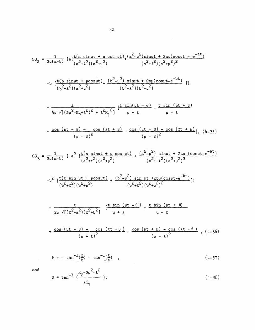
+ 1 [t sin(~t - £) t sin (~t + 8)
4~ 1[(2~2-K2+t2 ) 2 + t2~2 ) ~ + i ~ - i
+ cos (~t - 8) - cos (it + 8)
(~ - i)2
-b2 [t(b sin ~t + ~cos~t)
(b2+i2 )(b2 +i)
cos (~t + 8)- cos (it+ 8)], (4-35)
(~ - i)2
t [t sin (~t -e') t sin (~t + 6)
2~ l[(i2+a2 )(i2+b2 ] u + i u- i
+ cos ( ~t - B) - cos (it + 6 )
(~ + i)2
'
cos (~t + 8)- cos (it +6) ' (4-36) (~ - 1)2
( 4-37)
(4-38)
31
4.4 Discussion of the Solution
Difficulties in finding the inverse Laplace transform of
an expression are usually related to the degree and complexity of the
polynomial in its denominator. In our case the denominator is
basically given by the analytical expression for the determinant of
the Q-matrix. Therefore the order of the dynamics matrix F and the
complexity of its elements will to a large extent determine if the
use of this technique is advisable.
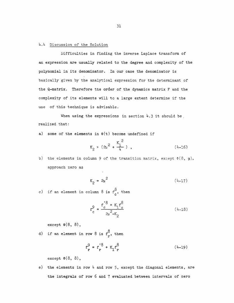
When using the expressions in section 4.3 it should be
realized that:
a) some of the elements in ~(t) become undefined if
(4-l6)
b) the elements in column 9 of the transition matrix, except ~(8, g),
approach zero as
K2 + ~2 ( 4:-17)
c) if an element in column 8 is f8 c' then
f9 f' 8 + K f 8
= c 1 c c 2
2ll -K 2
(4-18)
except ~(8, 8),
d) if an element in row 8 is f8 r' then
( 4-19)
except ~ ( 8, 8) ,
e) the elements in row 4 and row 5, except the diagonal elements, are
the integrals of row 6 and 7 evaluated between intervals of zero

32
and t.
In an undamped system the values of K1 and K2 are zero. The
inverse Laplace transform of the matrix N2 (4-8) becomes
cosh ~ sinh ~ c
L-lN = (4-20) 2 ~2 sinh ~ cosh /8;
c
The values of the elements in ~(t) which are associated with
the height channel increase exponentially as t increases. The increases
in these elements are propagated to each element in the transition
matrix, as indicated by equation (4-5), (4-6) and (4-7) and contaminate
the sinusoidal behaviour of the elements associated with the horizontal
channels when the value of t becomes very large.

5. S::ERIES SOLuriON
The series expansion approach is another way to find the
solution of the transition matrix of equation (2-2). The dynamics
matrix F can be substituted into equation ( 2-8) to form an
infinite series representation for the transition matrix t(t) which
converges for all values oft. Each element in the matrix is expressed
in form of a Taylor series expanding around the point where time t is
zero. By examining and regrouping the corresponding variables in each
series, the elements in the transition matrix may be expressed as sums
of several less complicated Taylor series of co~n functions. The
analytical expressions for the elements in the transition matrix may then
be derived from these series. However, this approach for the solution
of the transition matrix can be a very lengthy and difficult process.
The matrix t·{ t) has to be expanded analytically to the
sixth, or perhaps the seventh term of the series to include all the
essential components required to form the simpler series of
common functions. Regrouping the series is another difficult task.
Some of the series may not be easily rearranged to become sums of
common functions. The final analytical expression for the matrix t(t)
derived in the series expansion approach are listed in section 5.2 ..
33

5.1 Basic Technique
Two of the series approximations of elements of ~(t ) are
derived here to show how the series were rearranged to get the final
expressions.
The series expansion of element ~(1, 1) is
~(1, 1) t 2 2 . 2 2 t 4 4 2 4 2 2 = 1- ~ (i s~n ~ + ~) + 24 (i sin~+~ + ~ i) ••.
= r n=O
Using the assumption that
(5.1) may be reduced to
~(1, 1) = cos ~t + sin2~ (1 - cos it) .
Another element ~(2, 9) can be represented by the series
4 2 • • 3 2 t ( K2-~ ) <I> tel> t i sin 2p + ~ ( 2 ' 9) = R - -=--~3R~=-~ --1.::.2R..,....__
t5 2 12 t6 (K -~2)2~ (K2-4~ ) sin 2~ 2 + + R 360R
7 2 5~2) 12 t ['tK2-~ )Kl sin 2~ + . . . .
5040R
It can be rearranged and yields
(5-1)
(5-2)
(5-3)
(5-4)
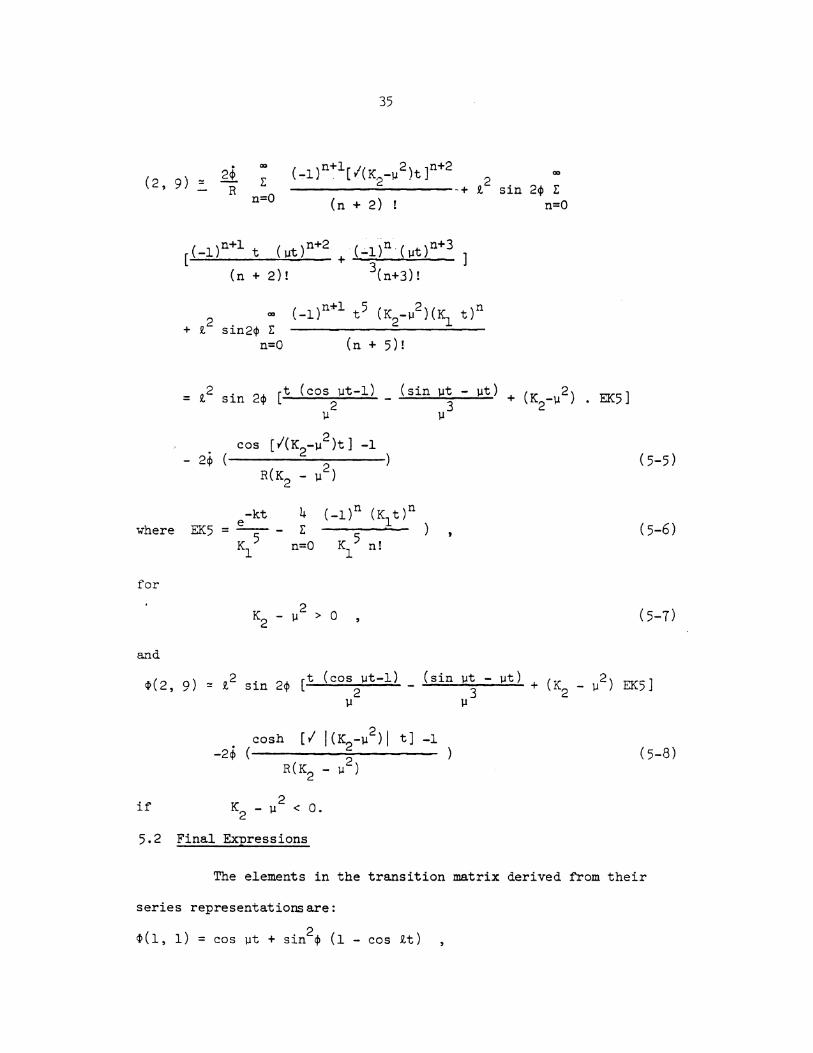
35
( 2' 9) I: n=O
(~l)n+l[I(K2-~2)t]n+2 ~ ----------+ t 2 sin 2cp I:
where
for
and
(n + 2) ! n=O
[(-l)n+l t (~)n+2 + (..;.1 )n·('llt)n+3
(n + 2)! 3(n+3)!
~ (-l)n+l t5 (K2-'Il2)(Kl t)n + R. 2 sin 2cp I:
n=O (n + 5)!
.2 t (cos 'llt-1) = ~ sin 2cp [ 2 (sin 'llt - 'llt) + (K -'112) • EK5 ] '113 2
- 2~
'll
cos [I(K2-'Il2 )t] -1
2 R(K2 - 'll )
-kt 4 e
(-l)n (K t)n 1 ) EK5 = --- I:
K 5 n=O l
K - '11 2 > 0 2
K 5 n' l .
(5-5)
(5-6)
(5-7)
~( 2' 9) (sin 'llt - 'llt) 2 ~;.;;;;;....,~---'"'"""'- + ( K2 - 'll ) EK5 ]
'll3
(5-8)
if
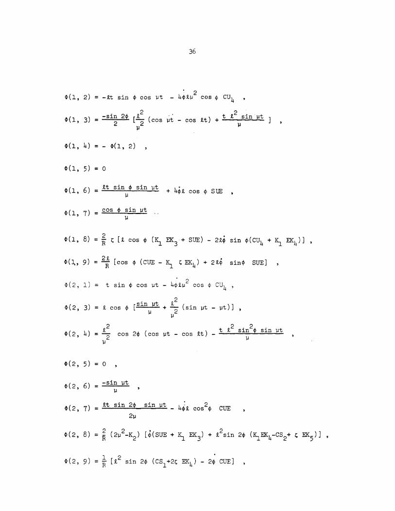
5.2 Final Expressions
The elements in the transition matrix derived from their
series representations are:
~(1, l) = cos 'llt + sin2cp (1 - cos R.t)
36
. 2 ~(1, 2) = -1t sin <1> cos lJt - 4<1>1JJ cos <f> cu4
· 2.~, i t 12 .sin·JJt ~( 1, 3) = -Sl.~ 'f' [ 2 (COS ~t - COS R.t) + ---.;~=;;o...:....;;. 1J J.l
~(1, 4) = - ~(1, 2)
~(1, 5) = 0
~(1, 6) R.t sin p sin )Jt + 4¢R. cos <I> SUE = )J
~(1, 7) cos 4> sin )Jt = 1J
~(]., 9) = 2: [cos <1> (CUE - IS_ l; EK4 ) + 21$ sin<l> SUE]
~(2, 1) . 2
= t sin <1> cos JJt - 4<t>iJJ cos <1> cu4
~(2, 3) [ sin )Jt 12 = R. cos <f> + 2 (sin lJt - lJt) ]
lJ lJ
12 t 12 sin2 <1> sin )Jt ~ ( 2' 4) = 2 cos 2<1> (cos )Jt - cos 1t) - ""'-""'--..;;;;.;)J--.... _______ ___ )J
~(2, 5) = 0
~(2, 6) -sin J.lt = )J
~( 2 , 7 ) = R.t sin 24> sin )Jt _ 4~ 1 cos2<1> CUE
2)J

37
~(3, 1) =tan ~(1 -cos ~t) - sin~ cos ~ (cos it-1) ,
~(3, 2) = sec ~(it sin2~ cos ~t - sin it)
~(3, 3) = cos2~ sin2~ cos it ,
~( 3, 4) n • 2 .1. • t = sec ~ ( .:;:.~v.....:S:..:J.:::n~r~;.....;::.s.::.:J.n::.....::~:.::.. - sin it )
~
~(3, 5) = 0
~(3, 6) = -tan ~ ~(1, 6)
~(3, 7) =-tan cp ~(1, 7)
~(3, 8) = -tan ~ ~(1, 8)
¢(3, 9) = -tanq, 1> (1, 9)
~(4, 1) = sin~ (sin it - it cos~t)
~(4, 2) = 1 - cos ut ,
~(4, 3) = i cos p( ut - sin ~t)
~
~(4, 4) = 1
~(4, 5) = 0
~(4, 6) = ~(2, 6) '
~(4, 7) = -~(2, 7)
~ ( 4 ' 8) = -~ ( 2 ' 8)

~(4, 9) = - ~(2, 9)
~(5, 1) = sin ~(cos ~t - 1)
~(5, 2) = sec ~ t(4, 1)
~ ( 5' 3) [1 - cos .12
cos ~t) t = sin ~ 1t + 2 (1-
~
~(5, 4) = R. tan ~( ~t - sin lit)
~
~(5, 5) = 1
~(5, 6) = sec $ ~(1, 6)
~(5, 7) = sec ~ ~(1, 7)
~(5, 8) = sec ~ ~(1, 8)
~ ( 5, 9) = sec ~ ~ ( 1, 8) ,
~(6, 1) = R. sin ~(cos tt - cos ~t + ~t sin ~t) ,
2 ~(6, 2) = ~ sin ~t +!_(sin ~t - ~t)
~
~ ( 6 , 3) = R.. COS ~ ( 1 - COS ~ )
t 2 2 2
12 sin~t ] ~
~(6, 4) =-- (sin ~t - ~t) + 1 sin ~ (t cos ~t - sin vt ) \J 'I' ~ '
~(6, 5) = 0
'
~(6, 7 ) = -4~R. cos2$[t sin JJt + ~ EK) 1 sin 2$ (sin ~t + ~t cos ~t)~ 2~ 3 - 2~

( . · 2 . 2 sin ut - ut ~(7, 1) = - sec ~ u nn lJt + R. s~n ~ .=;.......:;;;.;;_-....:;;~
lJ
~(7, 2) = R. tan ~(cos R.t- cos ut + lJt sin lJt)
~(7, 3) = R. sin ~(sin lJt- tt cos lJt)
t t 2 sin gt ~(7, 4) = R. tan ~(cos R.t- cos u + 2u )
~{7,5)=0,
~(7, 6) =; tan ~(sin ut + ut cos ut) - 4~t (0.5 SH2 - K1~ EK4)
~tB, 1) = 2Rtu2 [cos ~(SUE+ KIEK3) + 2~ sin ~(cs2+1.5KIEK4+1.5~EK5 )] ,
2 . 2 2 ) . 2 ~(8, 2) = Rt s~n ~ [3u (KlEK4 + ~EK5 + 2CS2] - 2R~u (SUE + KlEK3) ,
• 2 2 2 2 ~(8, 3) = R1(2~u cos ~(~EK4 + CUE) + t sin ~ cos $(CS3-3Klll EK5
+ ict 7 } 1 1863
( 2 2 • 2 ~ 8, 4) = Rt u (sin 2~ {CUE + K1EK4) + 2~(1 + 2 sin $) EK4] ,

~u
~( 8' 5) = 0
~(8, 6) = 2R <P.[K EK -CUE- K (K -l) EK4)J- 2Ri sin2 q,(CS1+ EK4 1 2 1 2
( 8 8) . -K t [ ( ) ( ) ] ~ , = e 1 + CHE - 1 - ~ l;; t EK1 + z;EK3 + EK2 + 2r;;EK4
~(9, 1) = 2Rt~2 {cos $CUE+ ~sin q,(t( 1 -2co~ ~t) - 3l;; EK4]} ~
~( 9 , 2) = 2R~2 [¢ (1 - cos~t + r;;EK ) + i2 sin 2$( t- t cos~t 2 3 2
~ 2~
~(9, 3) = 2Rt~2 [¢ cos cp(~t - ;in ~t - r;EK4) + 3t2 sin q, cos2cp
2 cvt - t sin~t )]
4~3 + r;;EK5
~(9, 5) = 0
( ) 2 ) • t sin ~t ~ 9, 7 = 2Rt [cos q, (SN1 - ~ r;;EK3 - ¢ sin 24>( 2~ + l;;EK3)]
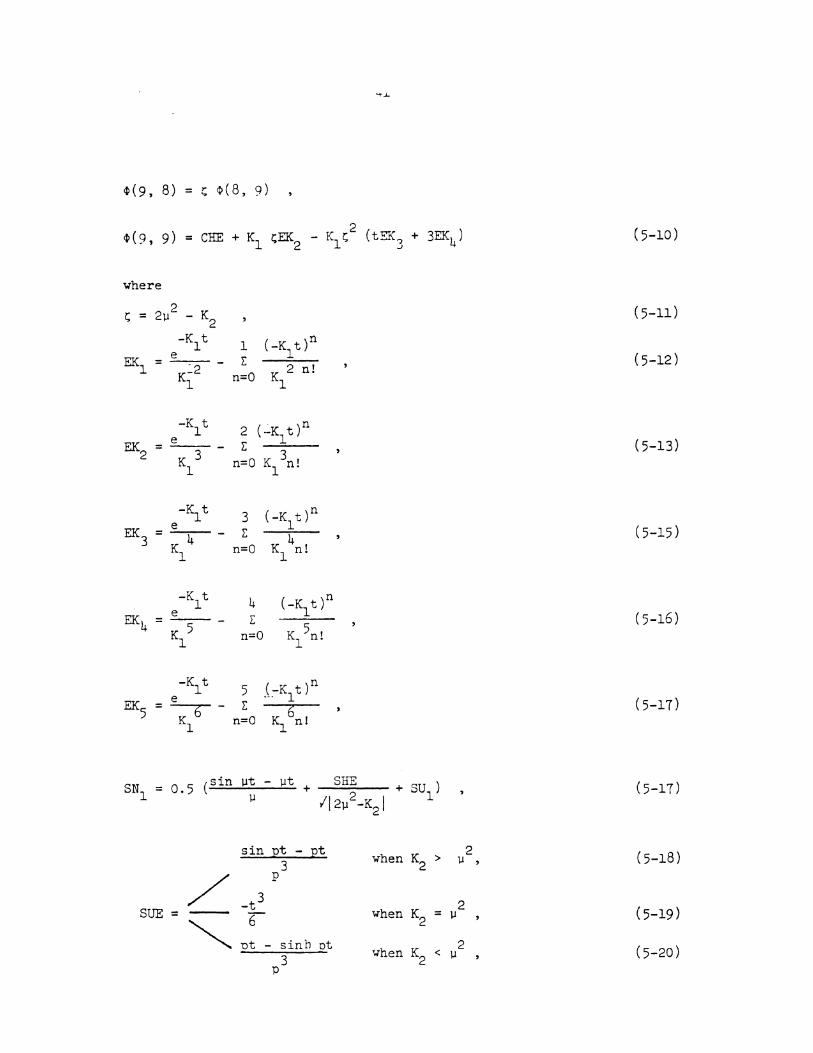
<11(9, 8) = ?; ¢(8, 9)
where
2 I;; = 2JJ - K
2
-K1t 1 (-K1t)n EK = _e __ - E
1 K~2 n=O K 2 n! 1 1
-K t 1
EK = _e __ -2 K 3
1
-K_t n -~ 3 ( -K1t)
EK = .::;.e~-- E 3 K 4 4
1 n=O K1 n!
-K t 1 e
EK4 = --K 5
1
4 E
n=O
sin pt - pt 3
SUE= / -t3 p
~ n:- sinh ot 3
p
2 when K2 > )J ,
2 = lJ
2 when K2 < ll
(5-10)
(5-11)
(5-12)
(5-13)
(5-15)
(5-16)
(5-17)
( 5-17)
(5-18)
(5-19)
(5-20)

sin pt /p su1 = -t
""sinh pt p p = I IK2 - ~PI
cos nt - 1 2 I K2 - "
-t2 CUE=--
2
\COSh Et - 1 2
K2 - \.1
cu4 = CUE+ G.5 t 2
K -2
2 \.1
.,., sin qt SHE =
"'-... sinh.qt
CHE = /cos qt
"-.....cosb qt
q = 112i - K2j
cs = t (cos \.1t - 1) 1 2
\.1
42
when K2 > \.1 2
when K2 = 2 \.1
when K2 < 2
\.1
when K2 >
when K2 =
when K2 <
2 when K2 .::_ 21.1
\.1
\.1
2 when K2 < 21.1 ,
2 when K2 .::_ 2\.1 ,
2 when K2 < 2\.1 ,
2 \.1
2
2
(5-21)
(5-22)
( 5-23)
(5-24)
(5-25)
(5-26)
(5-27)
(5-28)
(5-29)
( 5-30)
( 5-31)
( 5-32)
(5-33)

43
[t(sin )lt- lJt) 2(cos ut - 1 2 2
cs2 = 0.5 + +0.5ut 1 3
u )l (5-34)
t(cos )lt - 1 + 0.5 2 2 2(sin lJt -)ld t3
cs 3 u t = 2 3 3 )l 1J
(5-35)
and
t sin 1 + 2 -CHE SH2
ut 0. 5r,:t = • 1J 1;; (5-36)
5.3 Discussion of the Solution
The elements of the matrix given in section 5.2 were derived
from the first six terms of the series expansion of the transition
matrix ~(t). It was assumed that inferences on the high order terms
could be made from the first six terms. The other assumptions made in
deriving these expressions were the same as those made in the inverse
Laplace Transform approach. The expressions in the last two rows and
columns of the matrix are different from those derived in chapter 4
but they are numerically close.
The equations (5-17) to (5-32) indicate that for
2 K2 < ll
the expressions for elements associated with the height channel are
(5-39)
functions of hyperbolic functions which grow exponentially as t becomes
larger. Such growth can affect the other elements, espPcially those
associated with the velocity corrections, when t becomes very large.
Generally, the analytical expressions for the matrix ~(t)
derived in this chapter are shorter and less complicated than those
derived in chapter 4. However, it can be shown that many of the
expressions associated with the elements in the horizontal channels
are identical for both solutions. In most cases a series expansion

44
of the matrix elements given in section 4.3 will show this. The expressions
associated with the height channel are more complicated and their
agreement can only be shown by numerical comparison. The series
representation of the matrix exponential is less accurate because the
slimmation vas done on the basis of the first six terms only.
A~parently, theeff~ctsof some high order terms have been omitted by
this procedure.

6. TESTS AND NUMERICAL RESULTS
Two transition matrices have been derived in the last two
chapters. As has been pointed out in section 5.3 the equivalence of
the two solutions could not be shown analytically for each individual
element. Numerical tests were therefore performed for varying values
oft, $, K1 , and K2 in order to find out how closely the solutions
agreed numerically and how close they came to the exact solution. This
'exact' solution was computed by a numerical method given i:1 section 6.1
and it will be treated as the most accurate approximation to the actual
transition matrix. The differences between this matrix and the other
two matrices computed by using the analytical expressions of sections
4.3 and 5.2 will be regarded as the approximate errors of these
expressions.
6.1 The Numerical Method
The numerical method is basically the series expansion
solution. It generates the transition matrix ~(t ) by premultiplying n
a transition matrix for a small time interval t.t by itself for n times
t = n • t.t, n
(6-1)
where n is greater than zero. The matrix ~(t.t) can be computed by using
equation (2-8) truncated at a finite number of terms. The truncation
45

46
error is negligible if t:.t is very small. In our case t.t was equal
to 1 second and the matrix was truncated after the sixth term.
l'he Aolut.ton of the equation ( 2-2) for time t 1 may be vri tten as
~(tl) = 4>(t:.t, 0) . x(O) (6-2)
whe_re t, = t:.t ' ( 6-3)
-'-
and the solution for t is given by n
~(t ) = 4>(t ' tn-1) • ~(t ) n n n-1
4>(t ' tn-1) 4>(t t 2) ~(t = . n-1'
. n n- n-2
4>(tl, n + ( 6-4) = 0) • x(O)
for t = 0 (6-5) 0
Generating the solution with equation (6-4) is usually very time
consuming when the value of t becomes large. If the value of n is, n
however, a power of 2
k n = 2 , (6-6)
then the number of multiplications reduces from n to k. Formula ( 6-4)
is then replaced by
step 1 4>( t2) = ~(t:.t, 0)2
step 2 4>(t4) = ~(t2)2 = ~(t:.t, 0)4 • .. • • • 0 0 ..... ......
step k ~(t ) n = 4J(t )2 = ~(t.t, O)n (6-7)
n 2
Since we are usually free to choose t:.t the condition (6-6) can always be
satisfied. The major error in applying this method is the truncation
error occuring during the matrix multiplications.
\
)

6.2 Testing the Inverse Laplace Transform Solution
The solution for the transition matrix computed from the
analytical expressions given in chapter 4 was compared to the numerical
solution of the last section, for
25°~ ~ ~ 85° (6-8)
0 ~ Kl < f.! (6-9)
0 ~ K2 < 2
2].1 ' (6-10)
0 ~t <1000 seconds, ( 6-ll)
0 ~<P ~ 1. 31 X l0-5 rad/second (6-12)
and 0 ~>.. < l, 31 X l0-5 rad/second (6-13)
The results are given in the table below:
t)me (sec) max. percentage error
128 0.48
256 0.49
512 0.54
1024 1.13
Table 6-2 Error of Inverse Laplace Transform Solution
The inverse Laplace transform solution of the transition matrix
for the values of t between 1000 and 3000 seconds iras also computed to
show the effect of the damping loop gains K1 and K2 . The change of the
matrix elements ~(8, 8) and ~(9, 9) with respect to changes of K1
and K2 are tabulated in Table 6-2.
The results indicate that the values of ~(8, 8) and ~(9, 9)
increase rapidly for an undamped system.
The value of ~(8, 8) approaches e-Klt and the val~e of ~(9, 9)
becomes l. 0 as
(6-14)
and ~(8, 9) approaches t as
(6-15)

- -
time( sec.) 10000 1500 2000
K1 K2 t(8,B) t(9,9) t(8,8) 4>(9,9) 4>(8,8) 4>(9,9)
0 0 2.98 2.98 6.99 6.99 16.73 16.13
0. 211 o.4l 2.06 2.38 4.10 4.79 8.40 9.82
0. 4JJ o. 8\l 2 l. 39 1.91 2.29 3.26 3.98 5.70
0. 6ll l. 2ll 2 0.90 1.53 1.19 2.21 l. 71 3.27
o. 8ll l. 6ll 2 0.54 1.23 0.54 1.49 0.60 1.83
ll 2/ 0.29 1.00 0.155 1.00 0.08 1.00
lE-6 2ll 2 0.99 1.00 0.99 1.00 0.99 1.00 -
Table 6-2 Effect of Damping
2500
4>(8,8) 4>(9.9)
40.21 40.21
l7. 31 20.27
6.98 10.04
2.52 4.86
0.71 2.27
0.05 1.00
0.99 1.000
3000
4>(8,8)
96.69
35-73
12.30
3.74
0.86
0.02
0.99
4>(9,9)
96.69
41.84
17.60
7.23
2.81
1.00
1.00
I I
I .t:'" co
The values of other elements associated with the height channel also
decrease under the conditions (6-14) and (6-15). The numerical
method is generally a more time consuming way for generating a transition
matrix. In our case, the method required 10 times as much computation
time as the inverse Laplace transform solution to Dbtain the matrix
~(t) when t is larger than 128 seconds.
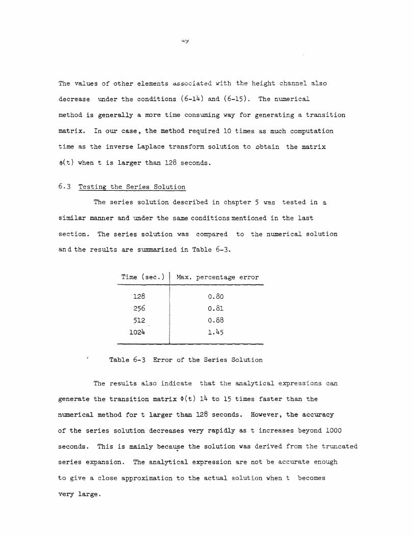
6.3 Testing the Series Solution
The series solution described in chapter 5 was tested in a
similar manner and under the same conditions mentioned in the last
section. The series solution was compared to the numerical solution
and the results are summarized in Table 6-3.
Time (sec.) Max. percentage error
128 0.80
256 0.81
512 0.88
1024 1.45
Table 6-3 Error of the Series Solution
The results also indicate that the analytical expressions can
generate the transition matrix ~(t) 14 to 15 times faster than the
numerical method for t larger than 128 seconds. However, the accuracy
of the series solution decreases very rapidly as t increases beyond 1000
seconds. This is mainly becaU?e the solution was derived from the truncated
series expansion. The analytical expression are not be accurate enough
to give a close approximation to the actual solution when t becomes
very large.
50
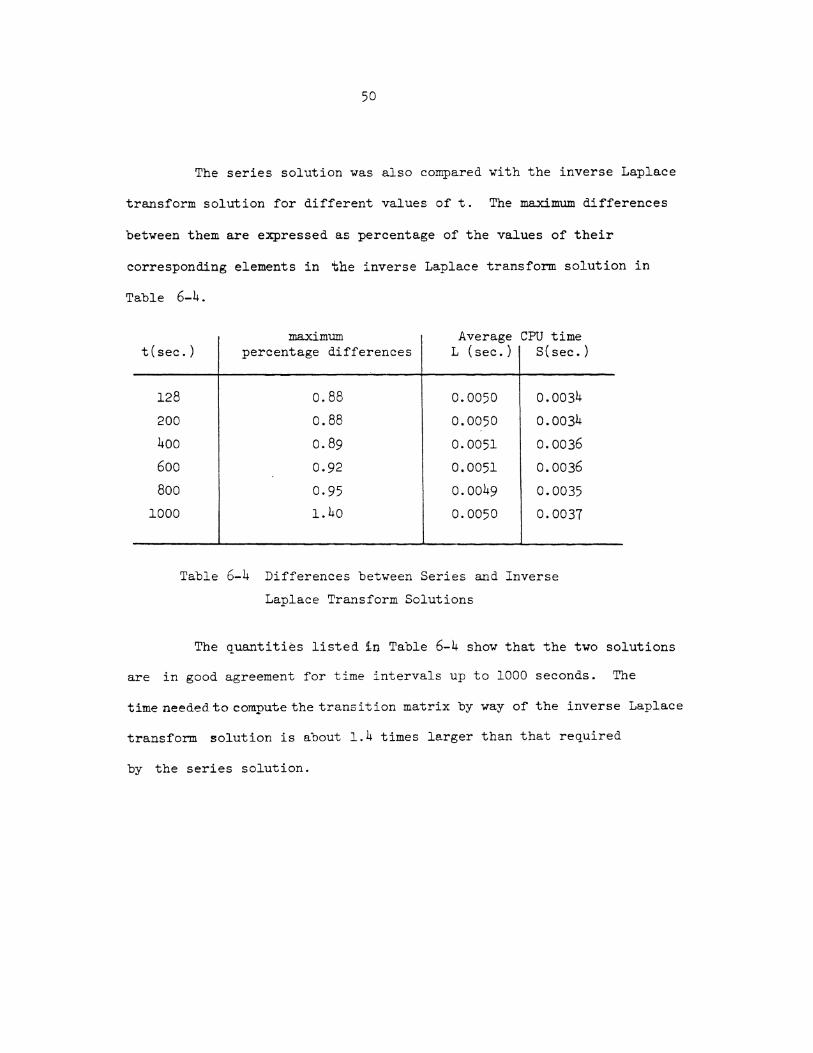
The series solution was also compared with the inverse Laplace
transform solution for different values oft. The maximum differences
between them are expressed as percentage of the values of their
corresponding elements in the inverse Laplace transform solution
Table 6-4.
maximum Average CPU time t(sec.) percentage differences L (sec.) S(sec.)
128 0.88 0.0050 0.0034
200 0.88 0.0050 0.0034
4oo 0.89 0.0051 0.0036
6oo 0.92 0.0051 0.0036
Boo 0.95 0.0049 0.0035
1000 1.40 0.0050 0.0037
Table 6-4 Differences between Series and Inverse
Laplace Transform Solutions
in
The quantities listed in Table 6-4 show that the two solutions
are in good agreement for time intervals up to 1000 seconds. The
time needed to compute the transition matrix by way of the inverse Laplace
transform solution is about 1.4 times larger than that required
by the series solution.
7. CONCLUSIONS
The analytical form of the transition matrix for the local
level case of inertial navigation has been derived in two different ways:
by using the inverse Laplace transform technique and by expanding the
matrix exponential into a series. The equivalence of the two solutions
can be shown for most matrix elements. Where it is not possible,
numerical comparisons have been made. The ~greement is always better
than 1.5% of the respective value for time intervals up to 1000 seconds.
Comparisons with an accurate nume~ical solution show agreement en the
same level of accuracy. For time intervals larger than 1000 seconds
the inverse Laplace transform solution is more accurate than the
series solution. Both analytical solutions are superior to the
numerical solution with respect to computer time by a factor of
10 to 15.
The analytical solutions can be used to discuss the
behaviour of individual errors in a very general manner and to spot
instabilities of the system. The best example is the instability
of the height channel. The expressions show that, in an undamped
system, the elements associated with the height channel contain
hyperbolic functions of the Schuler frequency and gro~ in exponenti~l.
manner when t becomes large. The damping loop gains, if properly
chosen, can reduce these errors.
51
52
The analJ~ical expressions were developed from a constant
dynamics matrix, i.e. by neglecting the time dependent components.
They can therefore only be treated as a first approximation to the
elements of the actual transition matrix of the system of error
equations. For further investigations, these time dependent
components may be included in the dynamics matrix. A better
approximation can then be obtained by using the inverse Laplace
transform solution as a first approximation and by deriving the
time dependent terms by a series expansion.

APPENDIX I
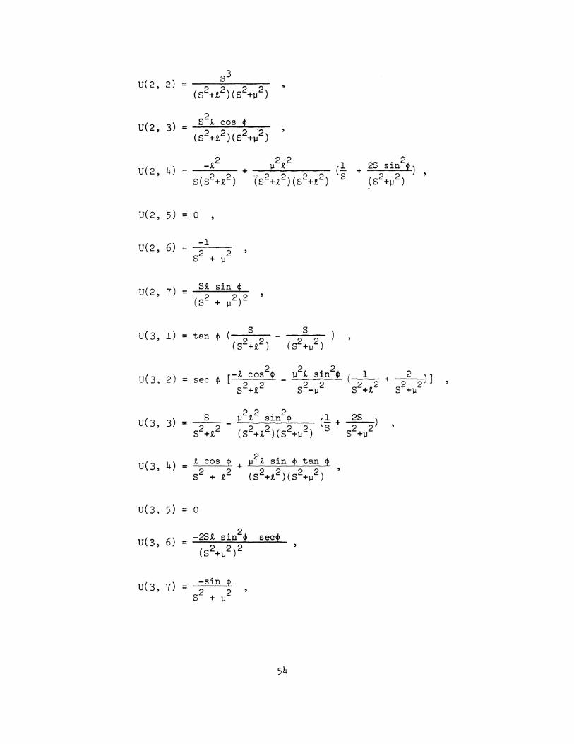
The purpose of this appendix is to show the elements of E2-l
in Chapter h and the detailed derivation of the matrix N2 described
in the same chapter.
Let us label E2 -l as U(Shhen the element in it are:
U(l, 1)
U( l, 2) ~ sin cp u 2 t sin<P ( 1 2 ) = + (8 2+t2) (82+ \l2) (S2H2) (S2+\l2) '
t 2 sin <P 1 2 1 2S ) ] U(1,3) ct>[
].L = cos + (- + S(S2H 2 ) (S2H2) (S2H.2) s (S2+l)
U( l, 4) = -s2 t sin cp
(S2H2)(S2+J.l2)
U(l, 5) = 0
U( 1, 6) = 2SR. sin cp
(s2 + u2)2
U(l, 7) = cos cp
(S2 + J.l2)
U( 2, 1) -R. sin cp + it sin <P ( 1 1
2 ) = + (S2 + 12) 2 2 (82 + t2) (S2 + (s + J.l ) ].l )
53
U( 2, 2) s3
= (S2+12)(S2+1J2)
2 U(2, 3) = 8 1 cos ~
(S2+12)(82+l)
U( 2, 4) -12 /12 cl + 2S sin2¢) = +
8(82+12 ) (82H2) (82+12) s (82+i)
U(2, 5) = 0
U(2, 6) -1
= 82 + 2
lJ
U( 2, 7) = SR. sin ~
(82 + i)2
U( 3, 1) = tan ¢ ( 8 s
(82+£2) ( 82+1J2)
2 J.! 2£ sin2¢ 1 2 U( 3, 2) = sec ¢ [-1 cos ¢ (22 + 22")]
S2H2 82+1J2 s +£ 8 +lJ
U(3, 3) s IJ2i2 sin2¢ (l + _g§__) =
82H2 (S2+£2)(S2+1J2) 8 82+lJ2
U( 3, 4) £ cos <P + 112£ sin ¢ tan ~ = 82 + 12 ( 8 2 H 2 ) ( 8 2 +IJ 2 )
U( 3, 5) = 0
U(3, 6) = -28£ sin2~ sec~
(82+i)2
u( 3, 7) = -sin <P
82 2 + l1
54

u(4, 1)
U(4, 2) =
U(4, 3) 2 = '.li cos 1>
(S2+.1'.2)(S2+'>l2)
U( 4, 5) = 0
U( 4, 6) = 1
82 + '>l2
U(4, 7) = SR. sin 2<j>
(S2 + u2)2
U(5, 1) =
2 U( 5, 2) = ];! i tan <j>
(S2+'>l2)
2£2 . U( 5, 3) = u s~n <j>
(s 2+t2 )(s2+·l)
2 U( 5, 4) = u II- tan <P
(S2+.1'.2)(S2+i)
U(5, 5) = s
U( 5, 6) = 2Si tan .p
(S2+ ll2)2
(1 -
( l 2 --+--) 32+.1'.2 S2+'>l2
(l+~) s 82 2 +'..!
2 (l - 2L-)
82+'..12
55

l U( 5, 7) = --=---
82 + i
U(6, l)
U(6, 2)
U(6, 3) =
U(6, 4) =
U( 6, 5) = 0
s U(6, 6) = -------
82 + ~ 2 +41 2 sin2 ¢
U(7, l) =
U(7, 2)
U( 7, 3)
U( 7, 5) = 0 ,
U(7, 6)
and
= 281. tan <P
(S2 + ~2)2
(AI-l)
56

Substituting the above matrices, A2 and c2 , into equation ( 4-4)
results in
. S+K. -1 I
= (D2-C2A2-~2) s + 4s(~2H2 2
K -21-1 2
Using the assumption that
l-12 » 9..2
and
2 ~2 ll >> ¢
(AI-2) may be reduced to
and its determinant is given by
where
and
= (S - a)(S -b)
I(K12 - 4K2 + 8})
(S2 + l-12)
2 cos p) (AI-2)
(AI-3)
(AI-4)
(AI-5)
(AI-6)
(AI-7)
(AI-8)
5 The matrix N2 may be derived by using standard co-factor techniques
s 1
( -1 ) -1 (s-aHS-b) (s-a)(s-b)
D2-C2A2 B2 = (AI-9) 2
21-1 -K2 S + K . .1
(S-a)(S-b) (S-a) (S-b)
57
REFERENCES
Adams, J.R. (1979): Description of the Local Level Inertial Survey System and its Simulation, Department of Survey Engineering. Technical Report No. 59, University of New Brunswick.
Bierman, G.F. (1971): Finite Series Solution for the Transition Matrix and the Covariance of a Time-Invariant System, IEEE, Transactions on Automatic Control Vol. AC-16, page 197-175.
Bellman, R. (1970): Introduction to Matrix Analysis, McGraw-Hill, New York.
Britting, K.R. (1971): Inertial Navigation System Analysis, WileyInterccience, New York.
Fossard, J.L. (1977): Multivariable System Control, North-Holland, Amsterdam.
Gantmacher, F.R. (1959): The Theory of Matrices,Vol. 2, Chelsea Publishing Company, New York.
Hochstadt, H. ( 19.75): Differential Equations, Dover Publishing Inc., New York.
KortUm, W. and Ho~an, W. (1974): Design of Optimal and Suboptimal State-Estimates under Regularity Defects, Deutsche. Luftund Raumfahrt, Forschungsbericht 74-73, Oberpfaffenhofen.
Lambert, J.D. (1977): The Initial Value Problem for Ordinary Differential Equations. In D.A.H. Jacobs (ed): The State of the Art in Numerical Analysis. Academic Press.
Lyon, F. (1977): Optimized Method for the Derivation of the Deflections of the Vertical from RGSS DATA, Proceeding of the '1st International Symposium on Inertial Technology ~or Surveying and Geodeys', Ottawa.
McCullum, P.A. and Brown, B.F. (1965): Laplace Transform Tables and Theorems, Holt, Rinehart and Winston, New York.
Moler, C. and Loan, Cb. van (1978): Nineteen Dubious Ways to Compute the Exponential of a Matrix. SIAM Review, Bd. 20, No. 4, s. 801-836.
Schmidt, G.T. (1978): Strapdown Inertial Systems- Theory and Applications - Introduction and Overview. AGARD Lecture Series No. 95.
58

Schwarz, K.P. (1979a): Inertial Surveying Systems -Experience and Prognosis. Paper presented at the FIG - Symposium on Modern Technology for Cadastre and Land Information Systems, Oct. 79, Ottawa. To be published in 'the Canadain Surveyor' 1980.
Schwarz, K.P. (1979b): Error Propagation in Inertial Positioning. Paper presented at the XVII General Assembly of the International Union of Geodesy and Geophysics, Canberra. To be published in 'the Canadain Surveyor', 3, 1980.
Spiegel, M.R. (1965): Laplace Transform, Schaum's Outline Series, McGraw-Hill Book Co , New York.
59
Recommended