IS-LM Revisited
Simple Income DeterminationProperties of IS & LM Curves
Equilibrium Output & Interest RatesEconomic Policy
(1) Simple Income Determination* Eco 1002
* Goods Market (IS)
* Exogenous Interest Rate & Prices
* Endogenous Income (GDP)
(2) IS-LM Model* Eco 2101 (Keynesian Short-Run)
* (1) + Money Market
* Endogenous Income & Interest Rate (Fixed P)
• Endogenous Policy
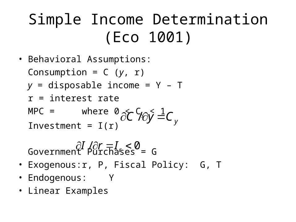
Simple Income Determination(Eco 1001)
• Behavioral Assumptions:
Consumption = C (y, r)
y = disposable income = Y – T
r = interest rate
MPC = where 0 < Cy < 1
Investment = I(r)
Government Purchases = G• Exogenous: r, P, Fiscal Policy: G, T• Endogenous:Y• Linear Examples
yCyC /
0/ rIrI
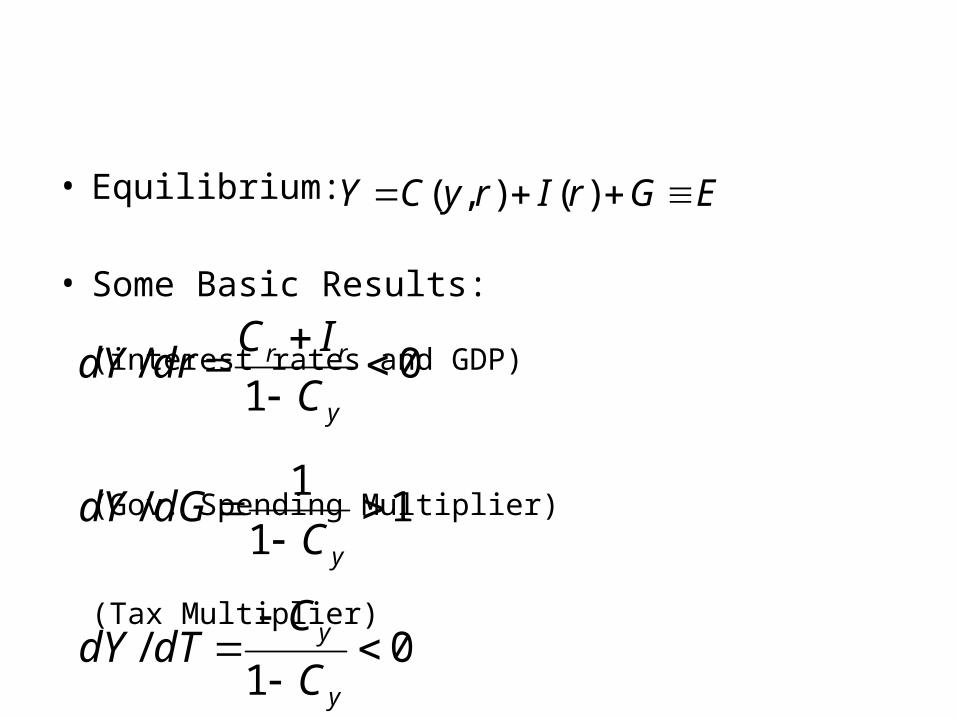
• Equilibrium:
• Some Basic Results:
(interest rates and GDP)
(Gov. Spending Multiplier)
(Tax Multiplier)
EGrIryCY )(),(
11
1/
yCdGdY
01
/
y
rr
C
ICdrdY
01
/
y
y
C
CdTdY
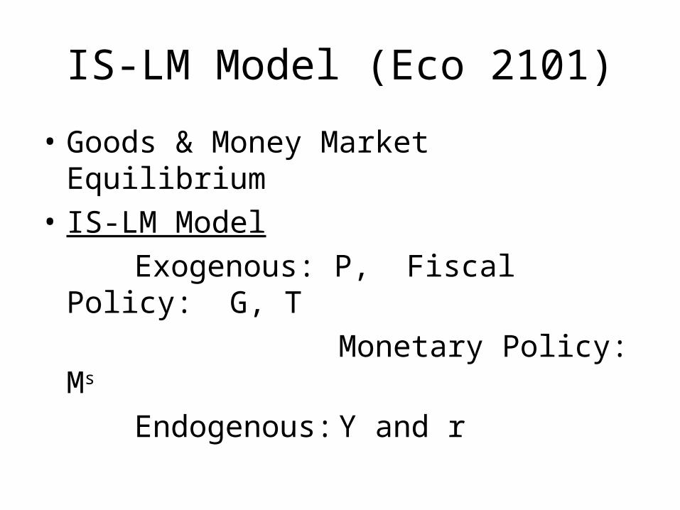
IS-LM Model (Eco 2101)
• Goods & Money Market Equilibrium
• IS-LM Model
Exogenous: P, Fiscal Policy: G, T
Monetary Policy: Ms
Endogenous: Y and r
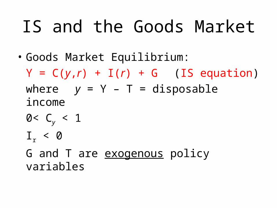
IS and the Goods Market
• Goods Market Equilibrium:
Y = C(y,r) + I(r) + G (IS equation)
where y = Y – T = disposable income
0< Cy < 1
Ir < 0
G and T are exogenous policy variables
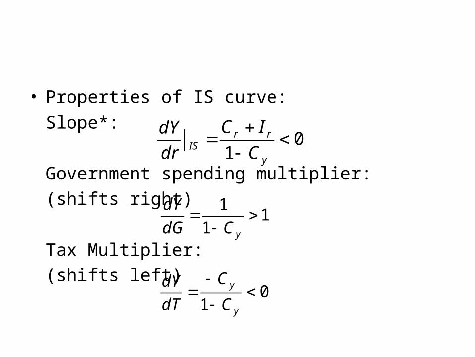
• Properties of IS curve:
Slope*:
Government spending multiplier:
(shifts right)
Tax Multiplier:
(shifts left)
01
y
rrIS C
IC
dr
dY
11
1
yCdG
dY
01
y
y
C
C
dT
dY
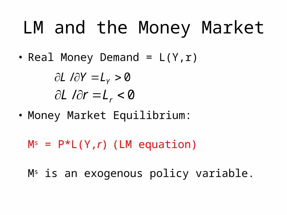
LM and the Money Market
• Real Money Demand = L(Y,r)
• Money Market Equilibrium:
Ms = P*L(Y,r) (LM equation)
Ms is an exogenous policy variable.
0/ YLYL
0/ rLrL
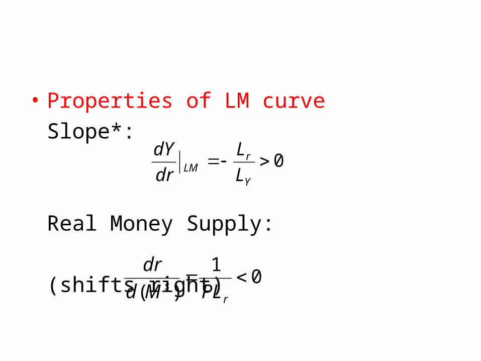
• Properties of LM curve
Slope*:
Real Money Supply:
(shifts right)
0Y
rLM L
L
dr
dY
01
)(
rs PLMd
dr
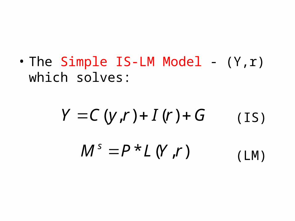
• The Simple IS-LM Model - (Y,r) which solves:
(IS)
(LM)
GrIryCY )(),(
),(* rYLPM s
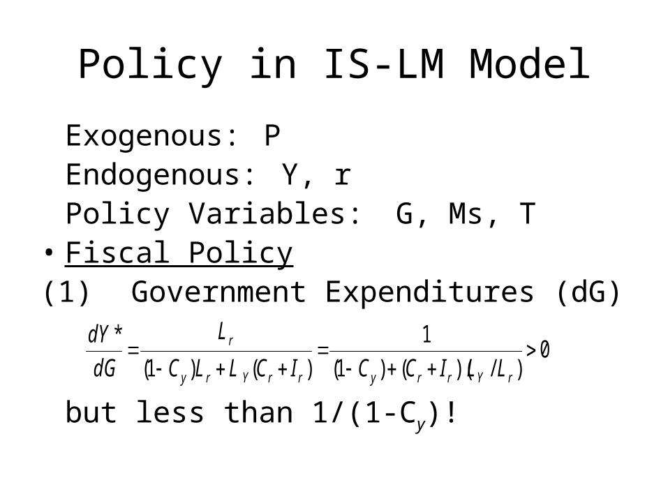
Policy in IS-LM Model
Exogenous: PEndogenous: Y, rPolicy Variables: G, Ms, T
• Fiscal Policy(1) Government Expenditures (dG)
but less than 1/(1-Cy)!
0)/)(()1(
1
)()1(
*
rYrryrrYry
r
LLICCICLLC
L
dG
dY
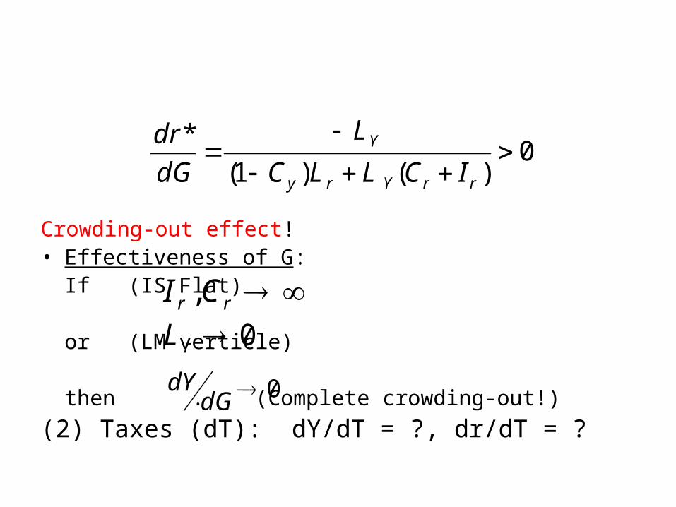
Crowding-out effect!• Effectiveness of G:
If (IS Flat)
or (LM verticle)
then . (Complete crowding-out!)
(2) Taxes (dT): dY/dT = ?, dr/dT = ?
0)()1(
*
rrYry
Y
ICLLC
L
dG
dr
rr CI ,0rL
0dGdY
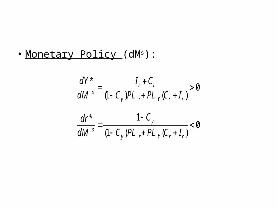
• Monetary Policy (dMs):
0)()1(
*
rrYry
rrs ICPLPLC
CI
dM
dY
0)()1(
1*
rrYry
y
s ICPLPLC
C
dM
dr
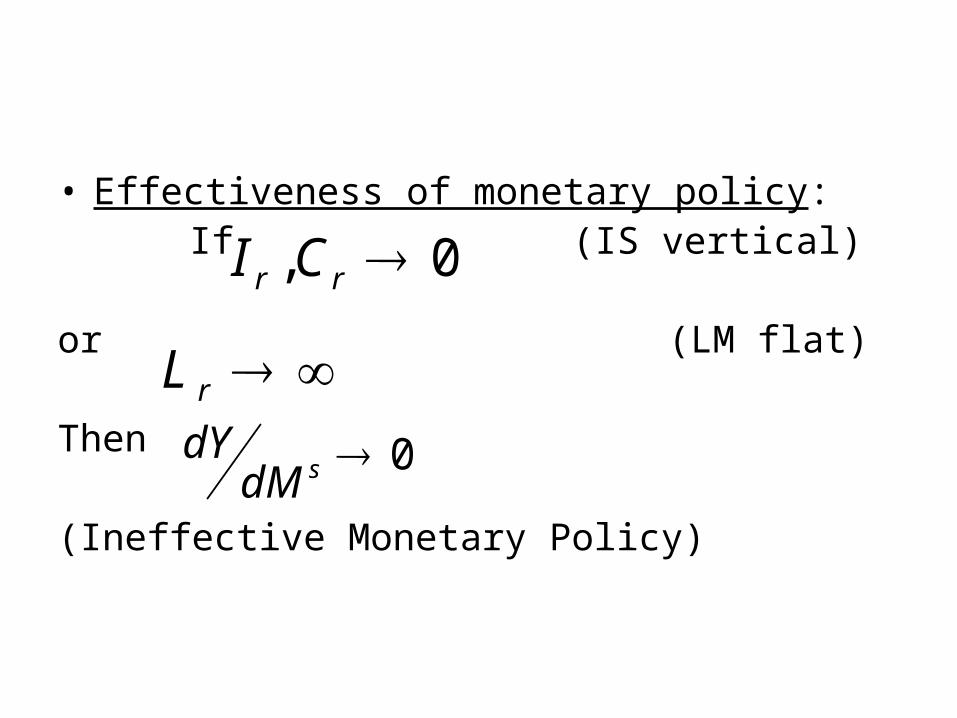
• Effectiveness of monetary policy:If (IS vertical)
or (LM flat)
Then
(Ineffective Monetary Policy)
0, rr CI
rL0sdM
dY
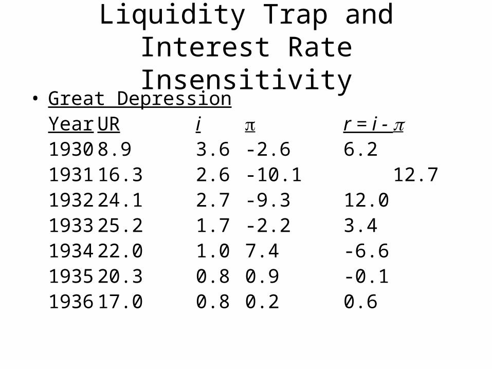
Liquidity Trap and Interest Rate Insensitivity
• Great DepressionYear UR i r = i - 1930 8.9 3.6 -2.6 6.21931 16.3 2.6 -10.1 12.71932 24.1 2.7 -9.3 12.01933 25.2 1.7 -2.2 3.41934 22.0 1.0 7.4 -6.61935 20.3 0.8 0.9 -0.11936 17.0 0.8 0.2 0.6
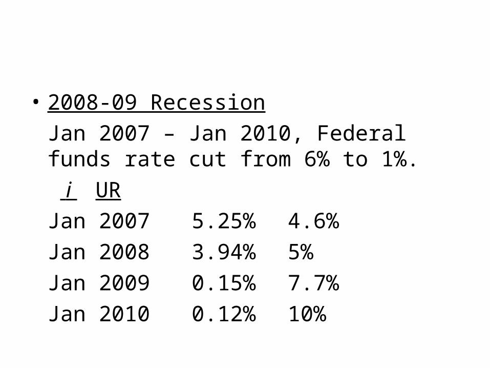
• 2008-09 Recession
Jan 2007 – Jan 2010, Federal funds rate cut from 6% to 1%.
i UR
Jan 2007 5.25% 4.6%
Jan 2008 3.94% 5%
Jan 2009 0.15% 7.7%
Jan 2010 0.12% 10%
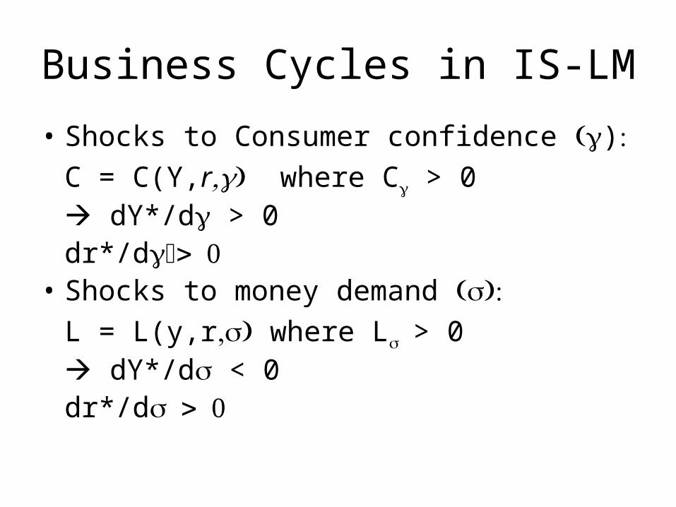
Business Cycles in IS-LM
• Shocks to Consumer confidence )C = C(Y,r where C > 0
dY*/d > 0dr*/d
• Shocks to money demand L = L(y,r where L> 0
dY*/d < 0dr*/d
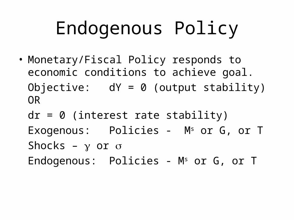
Endogenous Policy
• Monetary/Fiscal Policy responds to economic conditions to achieve goal.
Objective: dY = 0 (output stability) OR
dr = 0 (interest rate stability)
Exogenous: Policies - Ms or G, or T
Shocks – or
Endogenous: Policies - Ms or G, or T
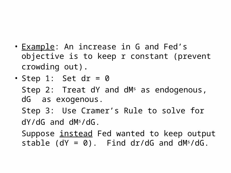
• Example: An increase in G and Fed’s objective is to keep r constant (prevent crowding out).
• Step 1: Set dr = 0
Step 2: Treat dY and dMs as endogenous, dG as exogenous.
Step 3: Use Cramer’s Rule to solve for
dY/dG and dMs/dG.
Suppose instead Fed wanted to keep output stable (dY = 0). Find dr/dG and dMs/dG.
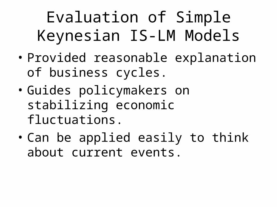
Evaluation of Simple Keynesian IS-LM Models
• Provided reasonable explanation of business cycles.
• Guides policymakers on stabilizing economic fluctuations.
• Can be applied easily to think about current events.
Shortcomings
• Criticisms of IS-LM Model:
(1) Emphasis on aggregate demand.
(2) Static Model.
(3) Lack of solid microeconomic foundations.
• Lucas Critique on Policy Evaluation
• Examples: Consumption, Phillips Curve
Modern Macro
• Dynamics
• Expectations (rational)
• Microeconomic Foundations
Most modern macro models (New Classical and New Keynesian) have these features.
Recommended