7/18/2019 jsee13_3 Response of Secondary System
http://slidepdf.com/reader/full/jsee133-response-of-secondary-system 1/17
JSEE: Summer 2004, Vol. 6, No. 2 / 29
ABSTRACT: A formulation for the response of the secondary systems subjected to multicomponent earthquake acceleration hasbeen developed, using the random vibration theory. The method accounts for interaction between the primary and the secondary systems as well as the nonproportionality of the combined primary- seondary system damping. The required formulations for thecalculation of the autocorrelation function, the power spectral density function, the response spectrum and the critical angle have beenobtained. The formulation has been arranged in such a way that the floor response spectrum can be calculated directly from the earthquakeresponse spectra of multicomponent input. The floor response spectraof torsional frames subjected to average response spectrum of 20earthquake records of Iran have been calculated. Variations of the spectra to various structure parameters such as eccentricity, mass ratio,and nonproportional damping have been studied. Results show that for large eccentricities the effect of multicomponentness of earthquakebecomes important and can not be neglected.
Keywords: Secondary Systems; Multicomponent earthquake;Interaction; Nonproportional damping; Mass ratio; Tunning
R esponse of Secondary Systems Subjected to
Multicomponent Earthquake Input
Mohsen Ghafory-Ashtiany 1 and A l i Reza Fiouz 2
1. International Institute of Earthquake Engineering and Seismology (IIEES), email:
2. Persian Gulf University, Boushehr, Iran
1. Introduction
For the modal analysis of important secondary
systems, it is common to generate the floor spectrum.
The floor spectrum defines the maximum absolute
acceleration response of a series of single degree of
freedom systems with different natural frequencies
and damping ratios, which are attached to the floor
under consideration. In the random vibration based
method, the spectral moments of the response of
floor is determined, and the floor spectrum is
calculated by multiplying its mean square by the
appropriate peak factor. Singh [1] used this method
and calculated the floor spectrum directly from the
design spectrum. In his method the input of the
secondary system was the response of the primary
system, so the interaction between the two systems
was neglected, and it was called decoupled (or
cascaded) analysis.Although the decoupled analysis is acceptable in
most cases, but there are situations which results to
significant overestimation, particularly when the
mass ratio is not too small, and the frequency of
the secondary system is tuned to one of the
predominant frequencies of the primary system. To
incorporate the effect of the dynamic interaction
between the two systems in the seismic analysis, the
secondary system can be considered as a part of
the whole structure and analyzed the combined
pri mar y-s ec on da ry sys tem by a conve ntion al
method. However, for light secondary systems, the
mass, damping, and stiffness matrices of the
combined system will have elements with much
smaller magnitude, which can cause numerical
instability in the dynamic analysis, resulting in the
numerical errors in the eigenvalue problem and
consequently on the response of the combined
system. Suarez and Singh [2] attempted to overcomethis shortcoming by presenting an exact approach to
determine the frequencies and mode shapes of the

7/18/2019 jsee13_3 Response of Secondary System
http://slidepdf.com/reader/full/jsee133-response-of-secondary-system 2/17
30 / JSEE: Summer 2004, Vol. 6, No. 2
M. Ghafory-Ashtiany and A.R. Fiouz
combined system. Because the mass of the secondary
system is usually small in comparison to the primary
system, it changes the dynamic properties of
the combined system slightly, so the perturbation
method become convenient to calculate the dynamic
properties and response of the combined system [3,
4, 5, 6]. Gupta and Tembulkar [7] studied the changesin both the frequencies and the response of the
primary and secondary systems due to decoupling.
Another problem in the analysis of the combined
system is due to the different damping characteristic
of the primary and secondary systems, which results
to the nonproportionality of the damping matrix. Thus
the analytical methods for the combined system
must be able to consider this effect. Direct and exact
method for calculating eigenvalues and eigenvectors
of nonproportionally damped systems, according to
the state vector approach, has been developed by
Foss [8], and after that has been used by many
researchers [9, 10]. Recently, new approach has been
developed by the first author, which substantially
reduces computational time [11].
In the seismic analysis of the secondary systems,
earthquake motion is commonly idealized as having
a single horizontal component, while in the actual
case there exist six correlated components (three
translational and three rotational), which are felt by
structure [12]. The rotational components can beexpressed in terms of the spatial derivatives of the
translational components [13, 14]. Three translational
components of earthquake are generally correlated,
but it can be found an orthogonal set of axis such that
the translational components are independent along
these axes. Kubo and Penzien [15] called these axes,
the principal axes of earthquake. Wilson and Button
[16] assumed that the two horizontal spectrum of
translational acceleration component of earthquake
are linearly dependent and proposed a complete
quadratic combination method for evaluating the
response of structure under these components.
Ghafory-Ashtiany and Singh [14] considered all of the
six components and calculated the response of
structure using the random vibration theory. Lopez
and Torres [17] considered structure as three-
dimensional frame with rigid floor that subjected to
the two horizontal component of the earthquake, and
determined the critical angle and the maximum
response of the structure.
A review of the existing literature shows that littleattention has been directed toward the effect of
torsion of the primary system on the response of the
secondary systems. Yang and Huang [18] presented
a complete quadratic combination rule to calculate
the response of the secondary systems, which are
attached to the torsional buildings, as well as the
effect of the base isolation system [19]. Bernal [20]
presented an example of a secondary system attached
to a torsional building.
In this paper the autocorrelation function, the
power spectral density function, and the floor
spectrum of the secondary systems, for which their
pr imary systems subjected to mult icomponent
earthquake have been formulated. In the presented
method, the interaction between the two systems and
the nonproportionality of damping of the combined
system is considered. The input of the primary
system can be in the form of time history with
correlated horizontal and vertical components of the
earthquake, power spectral density function or response spectrum of ground accelerations.
However, for the practical purposes, the formulations
are arranged such that the floor spectrum can be
calculated directly from the design spectrum at the
input level. Also the critical angle, i.e. the angle
between the axis of structure and the principal axes of
earthquake that produce maximum floor spectrum,
is calculated. In order to illustrate the applicability of
the method, torsional frames are considered and
parameters such as eccentricity, interaction, mass
ratio, and elevation of the secondary system from
ground, as well as nonproportional damping effect
have been studied.
To simplify the complex formulation for design
purposes, variation or sensitivity of each terms in the
formulation for different structural parameters have
been studied. The results of this study have been
presented in reference [21].
2. Formulation
Consider an N-degrees-of-freedom primary systemwith a mass [ M
p], damping [C
p], and stiffness matrix
[ K p
], attached by a single degree of freedom second-
ary system with a mass ( M s), a damping (C
s), and a
stiffness ( K s), to its mth degree of freedom, which
have been subjected to a multicomponent ground ex-
citation, .)( t x g ′&& The equations of motion of the com-
bined system become:
)(][
][][][][][ t x
r M
r M Y K Y C Y M g
s s
p p ′
−=++ &&&&&
(1)
Where Y = relative displacement response of
combined system and

7/18/2019 jsee13_3 Response of Secondary System
http://slidepdf.com/reader/full/jsee133-response-of-secondary-system 3/17
JSEE: Summer 2004, Vol. 6, No. 2 / 31
Response of Secondary Systems Subjected to Multicomponent Earthquake Input
=
s
p
M
M M
[0]
0][][ (2)
][0 [0]
0][][ c
p K
K K
+
= (3)
][0 [0]
0][][ c p C
C C
+= (4)
in which [ K c] and [C
c] are the coupling matrices
associated with the stiffness and damping matrices,
respectively, contain the stiffness and damping
coefficient of the secondary system in the mth and
N +1th element.
[ ]
−
−=
s s
s sc
K K
K K K
000
00000
000
00000
00000
LL
LL
MMMMMLL
MMMMM
LL
LL
(5)
[ ]
−
−=
s s
s sc
C C
C C C
000
00000
000
00000
00000
LL
LL
MMMMM
LL
MMMMM
LL
LL
(6)
In the present formulation it is assumed that the
earthquake has three translational correlated
components. Each row of )( t x g ′&& corresponds to an
acceleration component of earthquake along the
principal axes of the primary system, two horizontal
and one vertical axes [14, 15]. Also in Eq. (1), [r p
]
and [r s] are the displacement influence matrices
(matrices whose elements are the displacements of
degrees-of-freedom of the primary and the secondary
system, respectively, due to a unit static displacementof the base of the structure in the directions of
earthquake) of the primary and secondary systems.
These matrices have three columns, each column
corresponds to one component of the earthquake.
The eigenvalue problem of Eq. (1) in the case of
classical damped system is:
( [ K ] + ω2 [ M ] ) [φ] = [0] (7)
where ω and [φ] are the frequency and mode shape
of the combined system. For the light secondarysystems, the elements of [ K ] and [ M ] matrices are
not of the same order, which might cause numerical
inaccuracy. To overcome this shortcoming the
following transformation has been introduced [22]:
]][[][ U ϕ=ϕ (8)
where
ϕ
ϕ=
s
p
U ]0[
0][
][ (9)
in which [φ p
] is the mode shape of the primary system
normalized with respect to its mass matrix and
.1 s s M =φ Substitution of Eq. (8) into Eq. (7) gives:
]0[][][][ 2 =ϕω− M K (10)
where
][][][][ U M U M
T
= (11)
][][][][ U K U K T = (12)
The numerical inaccuracy of Eq. (7) has been
eliminated through the above mentioned trans
formation, since all diagonal elements of the matrices
in Eq. (10) are of the same order. However, two
sets of eigenvalue problems should be solved. First
for the primary system, and second the eigenvalue
Eq. (10).
Once the N +1 eigenvalues and eigenvectors of the
combined system are obtained, the equation of
motion, Eq. (1), can be solved using the normal
mode approach with the help of the following standard
transformation:
Y = [φ] V (13)
where V is the vector of principal coordinates.
Since [φ] is the normal mode shape of the system,
only the mass and the stiffness matrices could be
decoupled. Considering that the damping characteris-
tic of the primary and secondary systems aredifferent, the nonproportionality of damping matrix
is an inherent property of the coupled system. The
nonproportionality effect is particularly important for
the primary-secondary systems in tuning or nearly
tuning, with small values of mass ratio and large
differences in their damping constants. Substituting
Eq. (13) into Eq. (1) and premultiplying by [φi] leads
to Eq. (14):
∑
+
= ′γ −=ω++
1
1
2
][
N
i g j j jiij j xV V C V
&&&&&
; j=1, 2,…, N +1 (14)
where

7/18/2019 jsee13_3 Response of Secondary System
http://slidepdf.com/reader/full/jsee133-response-of-secondary-system 4/17
32 / JSEE: Summer 2004, Vol. 6, No. 2
M. Ghafory-Ashtiany and A.R. Fiouz
C ij
= φiT [C ] φ
j (15)
and
ϕ=γ
s s
p pT j j r M
r M
][
][][][ (16)
Eq. (14) is a coupled equation which can be
decoupled by using the state vector approach. The
state vector is defined as:
=
V
V Z
&
(17)
By using Eq. (17), Eq. (14) can be written as:
][
]0[][][][ g xQ Z B Z A ′
γ −=+ &&& (18)
where
=
−=
=
][]0[
]0[]0[][
][][
]0[][][
][][
][]0[][ 2 I
Q O0
I B
C I
I A
(19)
where [Ω 2] is a diagonal matrix of combined
frequencies, and [ I ] is the unit matrix of order N + 1.
To solve Eq. (18) by modal analysis, one should
find its eigenvalues and eigenvectors. The eigenvalue
problem of the Eq. (18) is:
(λ [ A ] + [ B ])[ψ ]=[0] (20)
Eq. (20) gives 2( N +1) eigenvalues (λ) and
corresponding eigenvectors [ψ ], which occur in the
pairs of complex and conjugate, due to negative-
definiteness of matrix [ B ]. Using the expansion
theorem, the vector Z is written as:
Z =[ψ ] x (21)
where Z is a vector of complex principal coordi-
nates. This vector is obtained by solving the Eq. (22):
][ g aaaa x F x x ′=λ− &&& ; a = 1, 2, …, 2( N +1) (22)
where
( ) aT
aT
aa AQ F ][][]0[
][][ ψ ψ
γ ψ −= (23)
in which F al
corresponds to direction l of the
earthquake.
The main response of the secondary system, which
is used for the generation of the floor spectrum, is the
absolute acceleration )( sU && which can be written in
terms of its relative acceleration )( sY && and the ground
acceleration component affecting it as:
][ g s s s xr Y U ′+= &&&&&& (24)
Using Eq. (13), the relative acceleration of the
secondary system can be written as:
∑+
=+ϕ=
1
11
N
j j j , N s V Y &&&&
(25)
Also by using Eqs. (17) and (21), we have:
∑+
=ψ == )(N
aa ja j j
x Z V
12
1
&&&& (26)
Obtaining a x& from Eq. (22) and substituting it into
Eqs. (26), (25) and (24), sU && will become:
′ψ ϕ+′
+
λψ ϕ=
∑ ∑
∑ ∑
+
=
+
=+
+
=
+
=+
1
1
1)2(
11
1
1
1)2(
11
][][
)(
N
j g a
N
a ja j , N g s
N
j
N
aaa ja j , N s
x F xr
t xU
&&&&
&&
(27)
Considering that the second terms in the right hand
side of Eq. (27) is zero, see Appendix (I), the absolute
acceleration of the secondary system will become:
( )∑ ∑+
=
+
=+
λψ +λψ ϕ=
1
1
1
11 )()()(
N
j
N
a
*a
*a
* jaaa ja j , N s t xt xt U
&& (28)
where superscript (*) means complex conjugate. Eq.
(28) forms the basis for the generation of floor
response spectrum. This will be used to calculate
the autocorrelation and power spectral density
function of the floor acceleration, which in turn is
required to define floor spectrum.
The autocorrelation function of the absolute
acceleration of the secondary system can be obtained
from Eq. (28) as:
(29)
In this equation, there are four expected values
which can be obtained in terms of autocorrelation or
power spectral density function of ground accelera-tion. Here, the first expected value in Eq. (29) will be
given as an example.
[ ]
[ ]
[ ]
[ ]
[ ]λψ λψ
+λψ λψ
+λψ λψ
+
λψ λψ
×ϕϕ=
∑ ∑
∑ ∑
∑ ∑
∑ ∑
∑ ∑
+
=
+
=
+
=
+
=
+
=
+
=
+
=
+
=
+
=
+
=++
1
1
1
121
1
1
1
121
1
1
1
121
1
1
1
121
1
1
1
11121
)()(
)()(
)()(
)()(
)()(
N
a
N
b
*ba
*b
*kba ja
N
a
N
b
*ba
*b
*kba ja
N
a
N
b
*b
*a
*b
*kb
*a
* ja
N
a
N
bbabkba ja
N
j
N
k k , N j , N s s
t xt x E
t xt x E
t xt x E
t xt x E
t U t U E
&&&&

7/18/2019 jsee13_3 Response of Secondary System
http://slidepdf.com/reader/full/jsee133-response-of-secondary-system 5/17
JSEE: Summer 2004, Vol. 6, No. 2 / 33
Response of Secondary Systems Subjected to Multicomponent Earthquake Input
To obtain the autocorrelation function xa, first we
need to solve Eq. (22) for xa in terms of Duhamel
integral.
( )∑ ∫ =
τ−λ ττ′=3
10
)()(l
t t gl al a
d e x F t x a && (30)
Using Eq. (30), E [ xa
(t 1
) xb
(t 2
)] becomes:
[ ]
[ ] 21)()(
21
3
1
3
10 011
2211
1 2
)()(
)()(
ττ′′
×=
−λ−λ
= =∑ ∑ ∫ ∫
d d eet xt x E
F F t xt x E
t t t t gn gl
l n
t t
bnal ba
ba &&&&
(31)
The relationship between the correlated accelera-
tions of earthquake along the principal axes of primary
system, , g x′&& and the uncorrelated accelerations
along the principal axes of earthquake, , g x&& is related
by the cosine direction matrix, [ D], as [15]:
][ g g x D x &&&& =′ (32)
where the acceleration cross correlation function can
be written as:
[ ] [ ]∑ ∑= =
=′′3
1
3
12121 )t()t()t()t(
p q gq gpnqlp gn gl x x E d d x x E &&&&&&&& (33)
in which p and q corresponds to the cosine direction
of the principal axes of the earthquake. Since the cross
correlation between accelerations along the principal
axes of earthquake is zero, the Eq . (33) can be
reduced to:
[ ] [ ]∑=
=′′3
12121 )t()t()t()t(
p gp gpnplp gn gl x x E d d x x E &&&&&&&& (34)
Expressing the autocorrelation function of the
ground accelerations in the Eq. (34), in terms of its
power spectral density function, and substituting it
into Eq. (33) and the result into Eq. (31), it becomes:
[ ]
( ) ( ) ( ) ωω
×=
∫ ∫ ∫
∑ ∑ ∑
∞+∞−
−ω−λ−λ
= = =
d d d eeeS
d d F F t xt x E
t t t t it t t t p
l n pnplpbnal ba
ba1 2 2122110 0 21
3
1
3
1
3
121
tt)(
)()(
(35)
Where S P
(ω) is the power spectral density function of
the ground accelerations along the pth principal axes of
earthquake. For the stationary processes, the limits of
integrals in Eq. (35) can be extended to −∞ and ,+∞and after some algebric calculation, the following is
obtained:
[ ]
∫
∑ ∑ ∑
∞+∞−
−ω
= = =
ωω+λω−λ
ω
×=
ba
t t i p
l n pnplpbnal ba
d ii
eS
d d F F t xt x E
)()(
)(
)()(
)(
3
1
3
1
3
121
21 (36)
Eq. (36) is the first used in the Eq. (29). The other
expected values, which can be obtained in similar
manner, are as follows:
[ ]
∫
∑ ∑ ∑
∞+∞−
−ω
= = =
ωω+λω−λ
ω
×=
ba
t t i
p
l n pnplp
*bn
*
*b
*a
d ii
eS
d d F F t xt x E
al
)()()(
)()(
**
)(
3
1
3
1
3
121
21
(37)
[ ]
∫
∑ ∑ ∑
∞+∞−
−ω
= = =
ωω+λω−λ
ω
×=
ba
t t i p
l n pnplp
*bn
*ba
d ii
eS
d d F F t xt x E
al
)()(
)(
)()(
*
)(
3
1
3
1
3
121
21 (38)
[ ]
∫
∑ ∑ ∑
∞+∞−
−ω
= = =
ωω+λω−λ
ω
×=
b*a
t t i p
l n pnplpbn
* ba
d ii
eS
d d F F t xt x E
al
)()(
)(
)()(
)(
3
1
3
1
3
121
*
21 (39)
Substituting Eqs. (36) to (39) into Eq. (29),
the total acceleration autocorrelation function
becomes:
With appropriate combination of the 1 st and 2n d
terms, and the 3rd and 4th terms, and after some
algebraic simplification, Eq. (40) can be rewritten as:
(40)
(41)
[ ]
ωω
ω+λω−λψ λψ λ
+ω+λω−λ
ψ λψ λ+
ω+λω−λ
ψ λψ λ
+
ω+λω−λ
ψ λψ λ
×ϕϕ=
−ω
∞+∞−
= = =
+
=
+
=
+
=
+
=++
∫ ∑ ∑ ∑∑∑
∑ ∑
d eS ii
F F
ii
F F
ii
F F
ii
F F
d d
t U t U E
t t i p
ba
bnkbb*al jaa
ba
*bnkbbal jaa
ba
*bnkbb
*al jaa
ba
bnkbbal jaa
l n pnplp
N
b
N
a
N
j
N
k k , N j , N s s
)(
*
**
*
**
**
****
3
1
3
1
3
1
1
1
1
1
1
1
1
11121
21)()()(
)()()()(
)()(
)()( &&&&
[ ]
( )
( )
( )
ωω
ωω+ω
+
ωω+ω
×
+
ω
×
ωω+ω
×ϕϕ=
−ω
∞+∞−
=
+
+= = = =
−ω
+
= = = =
∞+∞−
+
=
+
=++
∫
∑ ∑ ∑ ∑ ∑
∑ ∑ ∑ ∑ ∫
∑ ∑
d eS H DC
H B A
d d ?d eS H
B Ad d
t U t U E
t t i pbbnl jkabbnl jkab
aanl jkabanl jkab
N
a
N
ab l n pnplp
t t i pa
N
a l n panl jkaanl jkanplp
N
j
N
k k , N j , N s s
)(2224
2224
1
1
1
3
1
3
1
3
1
(2
1
1
3
1
3
1
3
1
224
1
1
1
11121
21
21
)(
2)(
)()( &&&&

7/18/2019 jsee13_3 Response of Secondary System
http://slidepdf.com/reader/full/jsee133-response-of-secondary-system 6/17
34 / JSEE: Summer 2004, Vol. 6, No. 2
M. Ghafory-Ashtiany and A.R. Fiouz
In which a H and b H are the complex frequency
function of the modes "a" and "b" of the combined
system, and the coefficients A jka ln
…, are defined in
Appendix (II). Eq. (41) defines the autocorrelation
function of the absolute acceleration of secondary
system. The power spectral density function of this
response will be:
]
(
) ])()(
)(
2
)()(
)(
2224
2224
1
1
1
3
1
3
1
3
1
2224
1 3
1
3
1
3
1
1
1
1
111
ωωω+ω
+ωω+ω
×
+ωωω+ω
×
ϕϕ=ω
∑ ∑ ∑ ∑ ∑
∑ ∑ ∑ ∑∑ ∑
=
+
+= = = =
+
= = = =
+
=
+
=++
pbbln jkabbln jkab
aaln jkabaln jkab
N
a
N
ab l n pnplp
paaln jkaaln jka
N
1a l n pnplp
N
j
N
k k , N j , N U
S H DC
H B A
d d
S H B A
d d S
s
&&
(42)
This equation defines the power spectral density
function of the absolute acceleration of the secondary
system in terms of the modal properties of the
primary system, eigenproperties of the combined
system, and the power spectral density function of
the ground accelerations along the principal axes of
earthquake.
For the stationary processes, the mean square
response of the total acceleration of the secondary
system can now be obtained through integration of
the response power spectral density function, Eq. (42):
[ ]
(
( )
)]
bb pbl ln jkab
bb pbln jkabaa paln jkab
N
a
N
ab l n p
aa paln jkabnplp
aa paln jkaaa paln jka
l n pnplp
N
1a
N
j
N
k k , N j , N s
I D
I C ? ,? I B
I Ad d
I B I A
d d U E
),(
),(
),((2
),(),((
][
12
04
12
1
1
1
3
1
3
1
3
1
04
12
04
3
1
3
1
3
1
11
1
1
111
2
ξωω
+ξωω+ω
+ξωω
+ξωω+ξωω
×ϕϕ=
∑ ∑ ∑ ∑ ∑
∑ ∑ ∑∑∑ ∑
=
+
+= = = =
= = =
+
=
+
=
+
=++
&&
(43)
Where I 0 p
(ωa, ξ
a) and I
1 p(ω
a, ξ
a), respectively,
represent the mean square values of the relative
displacement and relative velocity response of an
oscillator with frequency (ωa) and damping ratio (ξ
a)
excited by the ground motion in the p-direction. It is
a good approximation to suppose that the meansquare of the response are proportioned to the response
spectrum [23]; i.e.:
220 )()()( d aadp paa p PF / , Rd?S , I ξω=ω=ξω ∫
∞+∞−
(44)
2220 )()()( vaavp paa p PF / , Rd S , I ξω=ωωω=ξω ∫
∞+∞−
(45)
In which Rdp
(ωa, ξ
a) and R
vp(ω
a, ξ
a), are respectively,
relative displacement and relative velocity response
spectrum of ground motions in p-direction, and PF d
and PF v are the respective peak factors. Also, the
root mean square values of the absolute acceleration
of the secondary system when multiplied by the
corresponding peak factor will results to its response
spectrum:
][)( 222 sU s sU
U E F P , R
s s
&&&&&& =ξω (46)
Where )(2 s sU
, R s
ξω&& defines the total acceleration
floor spectra. Introducing Eqs. (43), (44), and (45)
into Eq. (46), and assuming that all the peak factors
are equal [24], the following result is obtained:
(47)( )[ ]
(
) ]ξω++ξω
×+
+ξω+
×ϕϕ=ξω
∑ ∑ ∑ ∑ ∑
∑ ∑ ∑∑∑ ∑
=
+
+= = = =
= = =
+
=
+
=
+
=++
),()(),(
)(2
),((
)(
22
1
1
1
3
1
3
1
3
1
2
3
1
3
1
3
1
11
1
1
111
2
bbapln jkabln jkabaaap
N
a
N
ab l n pln jkabln jkabnplp
aaapln jkaln jka
l n pnplp
N
1a
N
j
N
k k , N j , N s sU
R DC R
B Ad d
R B A
d d , R s&&
Where Rdp
(ωa, ξ
a) is the pseudo-acceleration
response spectrum of ground motions in p-direction.
Eq. (47) gives the relation for calculating floor
spectrum in terms of the cosine direction matrix [ D]
between the principal axes of earthquake and the
principal axes of the primary system. That is, if the
elements of this matrix are known, one can calculate
the floor spectrum. It is known that for most of the
tectonic regions, the ground motion can act along any
horizontal direction; therefore, this implies the exist-
ence of a possible different direction of seismic
incidence that would lead to an increase of floor
spectrum. Thus for important secondary systems, the
maximum response associated to the most critical
directions of ground motions must be examined.
The presented formulation is general and can be
applied to any structure and any direction of
earthquake, but here for avoiding the complexity of
the formulation, the primary system is restricted totorsional framed building with rigid floor that have
two perpendicular horizontal and one vertical degree

7/18/2019 jsee13_3 Response of Secondary System
http://slidepdf.com/reader/full/jsee133-response-of-secondary-system 7/17
JSEE: Summer 2004, Vol. 6, No. 2 / 35
Response of Secondary Systems Subjected to Multicomponent Earthquake Input
of freedom. Also, the earthquake is considered to
have two horizontal and one vertical component. For
this case the direction cosine matrix will become:
θθ−θθ
=100
0)()(
0)()(
scon si
n si sco
D][ (48)
whereθ is the horizontal angle between the principal
axes of earthquake and that of structure. Substituting
the elements of matrix [ D] in Eq. (47) gives:
0cs s
c s sU
R sincos R sin R
cos R R s
+θθ+θ+θ=ξω
)()()(
)(),(2
22&&
(49)
where
[
]
[
]),()(
),()(
),()(
),()(2
),()(),(
)(
222222
222222
211111
1
1
1
211111
222222
21
1111
11
1
1
111
bba jkab jkab
aaa jkab jkab
bba jkab jkab
N
a
N
abaaa jkab jkab
aaa jka jkaaaa
jka jka
N
1a
N
j
N
k k , N j , N c
S DC
S B A
S DC
S B A
S B A S
B A R
ξω+
+ξω+
+ξω+
+ξω+
+ξω++ξω
×+ϕϕ=
∑ ∑
∑∑ ∑
=
+
+=
+
=
+
=
+
=++
(50)
[
]
[
]),()(
),()(
),()(
),()(2
),()(),(
)(
212222
222222
221111
1
1
1
221111
212222
22
1111
1
1
1
111
bba jkab jkab
aaa jkab jkab
bba jkab jkab
N
a
N
abaaa jkab jkab
aaa jka jkaaaa
jka jka
N
1a
N
j
N
k k , N j , N s
S DC
S B A
S DC
S B A
S B A S
B A R
ξω+
+ξω+
+ξω+
+ξω+
+ξω++ξω
×+ϕϕ=
∑ ∑
∑∑ ∑
=
+
+=
=
+
=
+
=++
(51)
[
( )]
[
( )
( )]
bbabba
jkab jkab jkab jkab
aaaaaa
N
a
N
ab jkab jkab jkab jkab
aaaaaa jka jka
jka jka
N
1a
N
j
N
k k , N j , N cs
S S
DC DC
S S
B A B A
S S B A
B A R
),(),(
)(
),(),(
)(2
),(),()
(
21
22
21211212
21
22
1
1
121211212
21
221212
1212
1
1
1
111
ξω−ξω
×+++
+ξω−ξω
×+++
+ξω−ξω+
++ϕϕ=
∑ ∑
∑∑ ∑
=
+
+=
=
+
=
+
=++
(52)
[
[
]),()(),(
)(2),(
(
233333
23
1
1
13333
23
3333
1
1
1
1110
bba jkab jkabaaa
N
a
N
ab jkab jkabaaa
jka jka
N
1a
N
j
N
k k , N j , N
S DC S
B A S
B A R
ξω++ξω
×++ξω
×+ϕϕ=
∑ ∑
∑∑ ∑
=
+
+=
=
+
=
+
=++
(53)
Eq. (49) gives the floor spectrum as a function of the
angle of incidence (θ). The critical angle (θcr
) is
defined as the angle of incidence that causes the
maximum floor spectrum which can be obtained
from the derivative of ),(2 s s sU
R ξω&& with respect to θand by setting it equal to zero, it becomes:
sc
cscr
R R
Rtan
−=θ )2( (54)
This equation gives two roots for θcr
, with 90 o
difference, which defines the maximum and theminimum values of the floor spectrum. It should be
noted that the critical angle depends on the character-
istics of the horizontal spectra and the horizontal
dynamic properties of the structure.
From Eq. (52), it is known that if the two
horizontal ground spectrum are equal ( Rcs
= 0), then
θcr
= 0, which indicate that the floor spectrum does
not depend on the angle of incidence. For this reason,
it is enough to analyze the typical case of θ = 0 in order
to determine the maximum floor spectrum. In other
words, if the two horizontal ground spectra are
equal, the value of Rc is an upper bound of floor
spectrum to any angle of incidence.
3. Numerical Results
To demonstrate the application of the presented
method and to illustrate the importance of the
multi-components of the earthquake, a 10-story
torsional structure is considered to obtain the floor
response spectra for various parameters. The
dynamic properties of the structure are shown in
Figure (1) and its natural frequencies in the case of
zero eccentricities and without interaction and
nonproportional damping effects are listed in Table
(1). It is assumed that the eccentricity of stories are
equal in both directions.
In the presented formulation, the seismic input of
the primary system can be time history, power
spectral density function, or response spectrum of
ground accelerations. In this example the average
response spectra of 20 earthquake with similar characteristic, normalized to 1.0 g , is considered as
input. The two horizontal spectra are shown in

7/18/2019 jsee13_3 Response of Secondary System
http://slidepdf.com/reader/full/jsee133-response-of-secondary-system 8/17
36 / JSEE: Summer 2004, Vol. 6, No. 2
M. Ghafory-Ashtiany and A.R. Fiouz
Figure (2). For this structure the effect of eccentric -
ity, floor number, interaction, nonproportional
damping, and point of connection of the secondary
system on the floor, on the response of the secondary
system subjected to multicomponent earthquake
have been studied. The floor spectrum is obtained for
these different inputs:
i) The multicomponent earthquake acted along
the critical angle and its response will be denoted
by R.
ii) The single-component earthquake acted along
the critical angle and the floor spectrum and itsrelative difference with respect to R will be
denoted by R1 and e1, respectively.
Figure 1. Ten-story example structure.
Torsional Mode
Frequencies (rad/sec)
Lateral Mode
Frequencies (rad/sec)
Mode
Number
9.655.571
25.3914.662
41.5523.993
57.7233.324
71.3841.215
83.2348.056
90.8352.447
105.9361.168
116.5367.289
135.0877.9910
Table 1. Frequencies of the symmetric structure.
Figure 2. Input ground spectra.
iii) The single-component earthquake acted along
the principal axes of the primary structure and
the floor spectrum and its relative differencewith respect to R will be denoted by R
0 and e
0,
respectively.

7/18/2019 jsee13_3 Response of Secondary System
http://slidepdf.com/reader/full/jsee133-response-of-secondary-system 9/17
JSEE: Summer 2004, Vol. 6, No. 2 / 37
Response of Secondary Systems Subjected to Multicomponent Earthquake Input
3.1. Eff ect of Eccentr icity
Figure (3) shows the floor spectra at 10th floor for
eccentricity ratios of 5, 10, 15, and 20%. The
damping ratio of both the primary and the secondary
systems is assumed to be 0.02, and the mass ratio is
equal to 0.05. It is seen that as the eccentricity
increases, the response of the secondary system
and the difference between R , R1, and R0 will
increase. The increase in the tuning frequencies is
much larger than other frequencies. Thus, for
large eccentricities and in the tuning frequencies,
multicomponent effect should be considered.
3.2. Eff ect of I nteraction
The most important factor in the interaction is the
mass ratio of the secondary system to the floor. In
order to study the effect of interaction, four different
mass ratios is considered and floor spectrum of floor
Figure 3. Effect of eccentricity.

7/18/2019 jsee13_3 Response of Secondary System
http://slidepdf.com/reader/full/jsee133-response-of-secondary-system 10/17
38 / JSEE: Summer 2004, Vol. 6, No. 2
M. Ghafory-Ashtiany and A.R. Fiouz
5 have been calculated and plotted in Figure (4). In
this case the damping ratio of both the primary and
the secondary system are 0.05, and the eccentricity
is equal to 15%. From Figure (4), it can be seen that
by increasing the mass ratio, the floor response
spectrum will decrease, especially in the tuning
frequencies. Therefore interaction will be important
for heavy secondary system and tuning frequency.
This conclusion is in agreement with other research-
ers, such as Igusa and Derkiuregian [9]. Also from
this figure it can be seen that by increasing the
mass ratio, the difference between R, R1, and R0
will decrease and the error of neglecting multi-
componentness of earthquake decrease.
Figure 4. Effect of mass ratio.
7/18/2019 jsee13_3 Response of Secondary System
http://slidepdf.com/reader/full/jsee133-response-of-secondary-system 11/17
JSEE: Summer 2004, Vol. 6, No. 2 / 39
Response of Secondary Systems Subjected to Multicomponent Earthquake Input
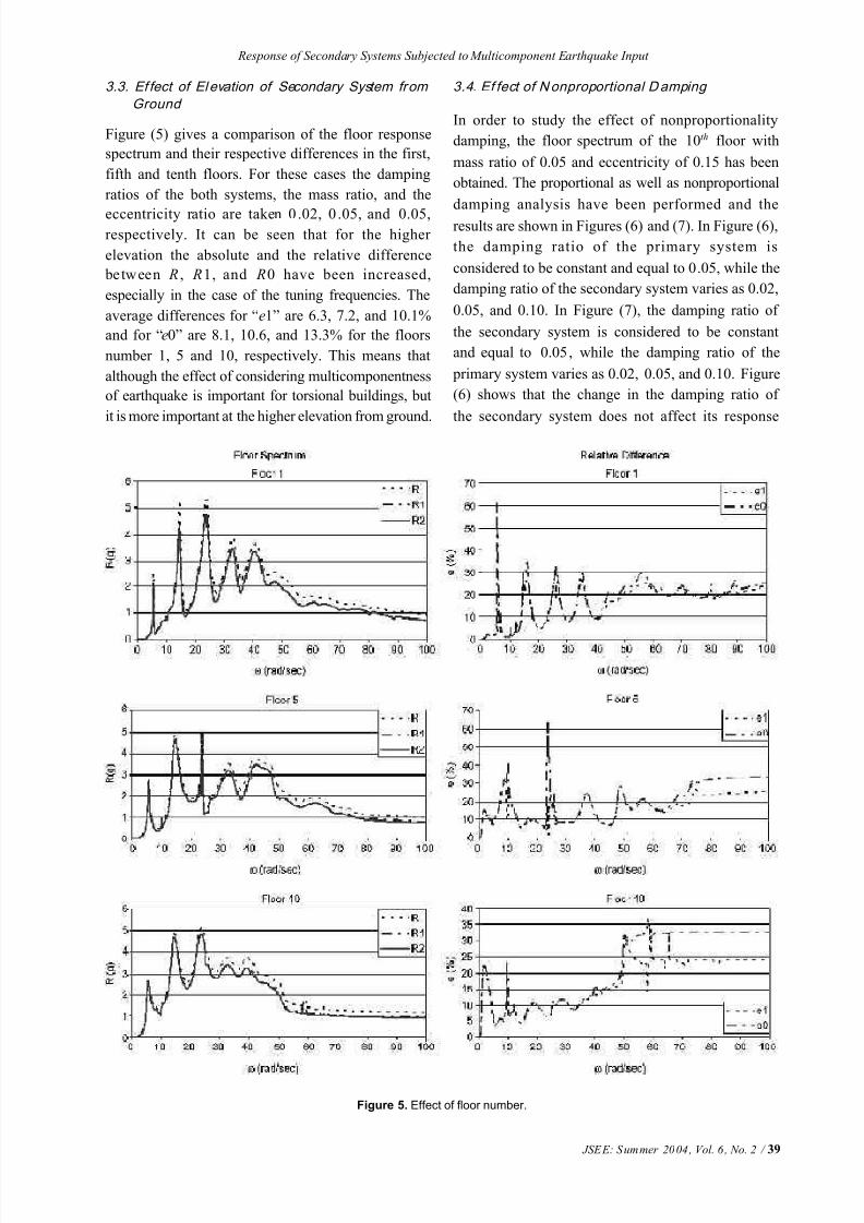
3.3. Ef fect of Elevation of Secondary System from
Ground
Figure (5) gives a comparison of the floor response
spectrum and their respective differences in the first,
fifth and tenth floors. For these cases the damping
ratios of the both systems, the mass ratio, and the
eccentricity ratio are taken 0 .02, 0 .05, and 0.05,respectively. It can be seen that for the higher
elevation the absolute and the relative difference
between R , R1, and R0 have been increased,
especially in the case of the tuning frequencies. The
average differences for “e1” are 6.3, 7.2, and 10.1%
and for “e0” are 8.1, 10.6, and 13.3% for the floors
number 1, 5 and 10, respectively. This means that
although the effect of considering multicomponentness
of earthquake is important for torsional buildings, but
it is more important at the higher elevation from ground.
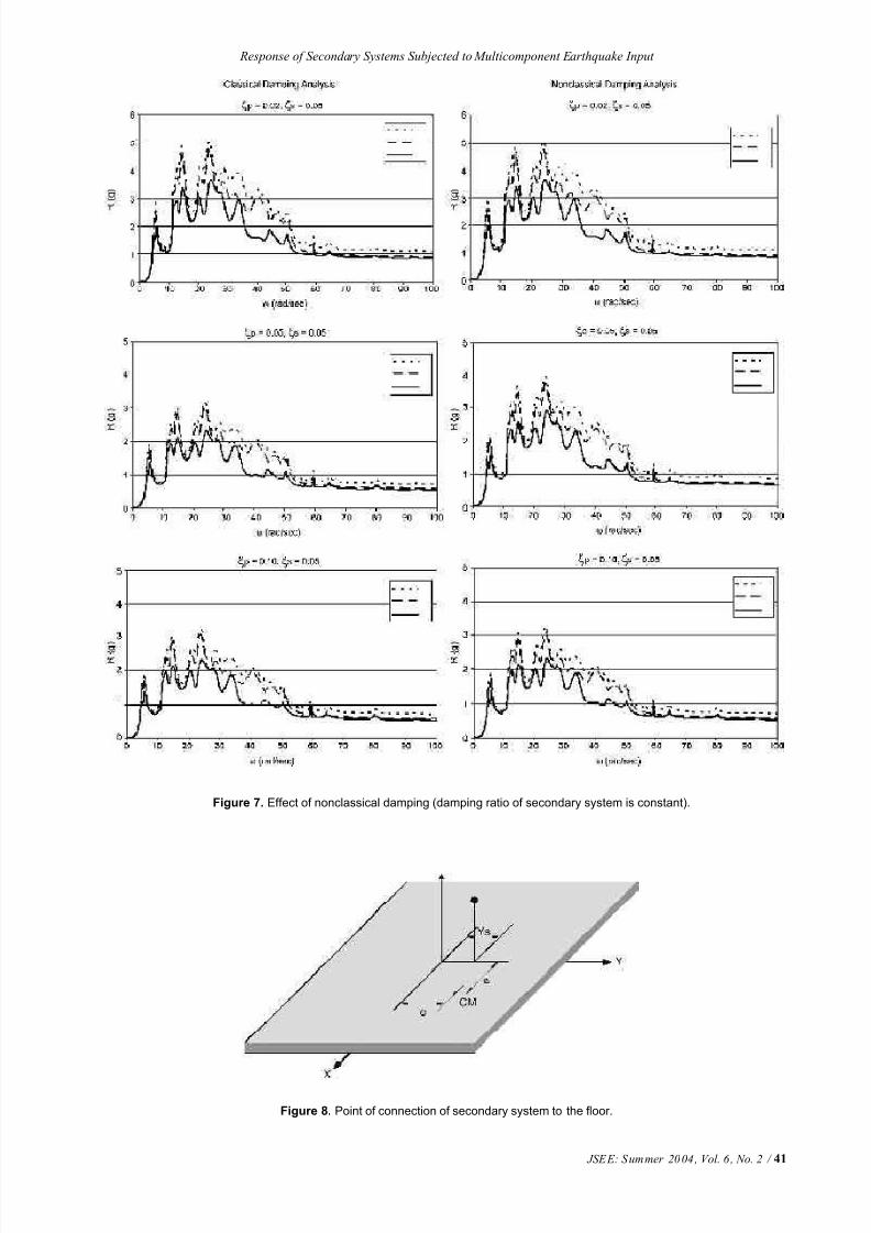
3.4. Ef fect of Nonproportional Damping
In order to study the effect of nonproportionality
damping, the floor spectrum of the 10th floor with
mass ratio of 0.05 and eccentricity of 0.15 has been
obtained. The proportional as well as nonproportional
damping analysis have been performed and the
results are shown in Figures (6) and (7). In Figure (6),
the damping ratio of the primary system is
considered to be constant and equal to 0.05, while the
damping ratio of the secondary system varies as 0.02,
0.05, and 0.10. In Figure (7), the damping ratio of
the secondary system is considered to be constant
and equal to 0.05, while the damping ratio of the
primary system varies as 0.02, 0.05, and 0.10. Figure
(6) shows that the change in the damping ratio of
the secondary system does not affect its response
Figure 5. Effect of floor number.

7/18/2019 jsee13_3 Response of Secondary System
http://slidepdf.com/reader/full/jsee133-response-of-secondary-system 12/17
40 / JSEE: Summer 2004, Vol. 6, No. 2
M. Ghafory-Ashtiany and A.R. Fiouz
Figure 6. Effect of nonclassical damping, damping ratio of primary system is constant.
significantly. But Figure (7) shows that the increase
in the damping ratio of the primary system cause the
decrease in the response of the secondary system.
This proves that the response of the secondary
system is affected by the damping ratio of the primary
structure rather than by the secondary system.
Figures (6) and (7) also show that the nonpropor-
tional damping analysis increase the response of the
secondary system, especially in the case of tuning
frequencies.
3.5.Ef fect of Point of Connection of the Second-
ary System on the F loor
The secondary system may be connected on a
location other than the center of mass of the floor as
it can be seen in Figure (8). In order to investigate
the effect of variation of the location of the
secondary system with respect to the center of
mass of the floor, the response spectrum of a
secondary system which installed on the 10th floor
with eccentricity of 0.01 has been obtained for
various ratios. The results have been shown in
Figure (9). A review of this figure shows that:
i) the response of the secondary system increases
as the ratio increases.
ii) the effect of multicomponent earthquake be-comes more important as the ratio between their
spectra or spectral density function increases.
7/18/2019 jsee13_3 Response of Secondary System
http://slidepdf.com/reader/full/jsee133-response-of-secondary-system 13/17
JSEE: Summer 2004, Vol. 6, No. 2 / 41
Response of Secondary Systems Subjected to Multicomponent Earthquake Input
Figure 8. Point of connection of secondary system to the floor.
Figure 7. Effect of nonclassical damping (damping ratio of secondary system is constant).

7/18/2019 jsee13_3 Response of Secondary System
http://slidepdf.com/reader/full/jsee133-response-of-secondary-system 14/17
42 / JSEE: Summer 2004, Vol. 6, No. 2
M. Ghafory-Ashtiany and A.R. Fiouz
Figure 9. Effect of point of connection of secondary system on floor.

7/18/2019 jsee13_3 Response of Secondary System
http://slidepdf.com/reader/full/jsee133-response-of-secondary-system 15/17
JSEE: Summer 2004, Vol. 6, No. 2 / 43
Response of Secondary Systems Subjected to Multicomponent Earthquake Input
4. Conclusions
New formulation for the calculation of the floor
response spectrum subjected to multicomponent
earthquake is presented, which accounts for the
interaction of the primary and the secondary systems
and nonproportional damping which are inherent
characteristics of combined systems. The autocorre-
lation, power spectral density functions, and mean
square responses have been also derived. The two
horizontal and one vertical components of earthquake
is considered and the critical angle, which produce
the maximum floor spectrum, has been obtained. The
proposed method is efficient, since it generates floor
response spectrum directly from the multicomponent
ground response spectra. Numerical studies show that
the effect of multicomponent earthquake input is
important in the structures with large eccentricity,
light secondary systems and in the case of tuned
modes.
References
1. Singh, M.P. (1975). “Generation of Seismic Floor
Spectra”, J. Eng. Mech., ASCE , 101(EM5), 593-
607.
2. Suarez, L.E. and Singh, M.P. (1987). “Seismic
Response of SDF Equipment-Structure System”,
J. Eng. Mech., ASCE, 113(1), 16-30.
3. Sackman, J.L. and Kelly, J.M. (1979). “Seismic
Analysis of Internal Equipment and Components
in Structures”, Eng. Str. , 1, 179-190.
4. Sackman, J.L., Derkiureghian, A., and Nour-Omid,
B. (1983). “Dynamic Analysis of Light Equipment
in Structures: Modal Properties of the Combined
System”, J. Eng. Mech., ASCE, 109(1), 73-89.
5. Derkiureghian, A., Sackman, J.L., and Nour-Omid,
B. (1983). “Dynamic Analysis of Light Equipment
in Structures: Response to Stochastic Input”, J.
Eng. Mech., ASCE, 109(1), 90-110.
6. Singh, M.P. and Suarez, L.P. (1986). “A
Perturbation Analysis of Eigenproperties of
Equipment-Structure Systems”, Nuclear Eng.
Des., 97, 167-185.
7. Gupta, A.K. and Tembulkar, M. (1984). “DynamicDecoupling of Secondary Systems”, Nuc. Eng.
Des., 81, 359-373.
8. Foss, K.A. (1958). “Coordinates which Uncouple
the Equation of Motion of Damped Linear
Dynamic Systems”, J. Appl. Mech., 25, 361-364.
9. Igu sa, T. and Derkiureghian, A. (1985).
“Generation of Floor Response Spectra Including
Oscillator-Structure Interaction”, Eq. Eng. Str.
Dyn., 13, 661-676.
10. Singh, M.P. and Suarez, L.P. (1987). “Seismic
Response Analysis of Structure-Equipment
Systems with Non-Classical Damping Effects”,
Eq. Eng. Str. Dyn., 15, 871-888
11. Khanlary, K. and Ghafory-Ashtiany, M.
(2004). “New Approaches for the Non-Classically
Damped System Eigenanalysis”, Accepted for
Publication in J. Earthquake Engineering and Structural Dynamics.
12. Rosenblueth, E.F. (1973). “The Six Components
of Earthquakes”, Proc. 12 th Regional Conf.
Planning and Design of Tall Buildings, Sydney,
Australia, 63-81.
13. Castellani, A. and Boffi, G. (1989). “On the
Rotational Component of Seismic Motion”, Eq.
Eng. Str. Dyn., 18, 785-797.
14. Ghafory-Ashtiany, M. and Singh, M.P. (1986).
“Structural Response for Six Correlated Earth-
quake Components”, Eq. Eng. Str. Dyn., 14, 103-
119.
15. Kubo, T. and Penzien, J. (1979). “Analysis of
Three-Dimensional Strong Ground Motions Along
Principal Axes, San Fernando Earthquake”, Eq.
Eng. Str. Dyn., 7, 265-278.
16. Wilson, E.L. and Button, M.R. (1982). “Three-
Dimensional Dynamic Analysis for Multi-
Component Earthquake Spectra”, Eq. Eng. Str.
Dyn., 10, 471-476.
17. Lopez, O.A. and Torres, R. (1997). “The Critical
Angle of Seismic Incidence and the Maximum
Structural Response”, Eq. Eng. Str. Dyn., 26, 881-
894.
18. Yang, Y.B. and Huang, W.H. (1993). “SeismicResponse of Light Equipment in Torsional
Buildings”, Eq. Eng. Str. Dyn., 22, 113-128.

7/18/2019 jsee13_3 Response of Secondary System
http://slidepdf.com/reader/full/jsee133-response-of-secondary-system 16/17
44 / JSEE: Summer 2004, Vol. 6, No. 2
M. Ghafory-Ashtiany and A.R. Fiouz
19. Yang, Y.B. and Huang, W.H. (1998). “Equipment-
Structure Interaction Considering the Effect of
Torsion and Base Isolation”, Eq. Eng. Str. Dyn.,
27, 155-171.
20. Bernal, D. (1999). “A Dynamic Stiffness Formu-
lation for the Analysis of Secondary Systems”,
Eq. Eng. Str. Dyn., 28, 1295-1308.
21. Fiouz, A.R. (2002) . “Analysis of Secondary
Systems Subjected to Multicomponent Earth-
quake Accelerations and Proposing Simplified
Methods”, Thesis Presented for Degree of
Philosophy in Structural Engineering, Tarbiat
Modarres University.
22. Suarez, L.E. and Singh, M.P. (1987). “Floor
Response Spectra with Structure-EquipmentInteraction Effects by a Mode Synthesis
Approach”, Eq. Eng. Str. Dyn., 15, 141-158.
23. Vanmarcke, E.H. (1976). “Seismic Structural
Response”, Ch. 8 in Seismic Risk and Engr.
Decisions, Ed. C. Lomnitz and E. Rosenblueth,
Elsevier Scientific Pub. Co., New York.
24. Ghafory-Ashtiany, M. (1983). “Seismic Response
for Multicomponent Earthquake”, Ph.D. Disser-
tation V.P.I. and S.U.
Appendix I
Since the secondary system is the N +1th degree of
freedom of the combined system, the parenthesis of
the second term of Eq. (27) can be written as:
∑ ∑=
+
=++ ′
ψ φ+
3
1
1
1,1,1 )(
l gl
N
jal ja j N l N x F r && (I-1)
If [Q] from Eq. (19) substitute in Eq. (23), [ F a]
becomes:
][
][
]0[
][
][
]0[
][]0[
]0[]0[
][a
T a
T a
aT
a
T a
a A A
I
F
ψ ψ
γ ψ −=
ψ ψ
γ
ψ
−= (I-2)
The l st element of [ F a] will be:
][
0
aT
a
l
T a
al A
F
ψ ψ
γ ψ −= (I-3)
The size of ψ a is 2( N +1) by 1, which can be
separated into the upper and lower parts:
ψ ψ =ψ
l la
ua
a
(I-4)
where uaψ and l
laψ are the ( N +1) upper and lower
element of ψ a, respectively. Substituting this
equation into Eq. (I-3), F al
becomes:
][
aT
a
l T l
aal
A F
ψ ψ γ ψ −= (I-5)
which can be written as:
][
0
][][
][]0[
aT
a
l
T
l a
ua
al A
C I
I
F ψ ψ
γ
ψ ψ
−= (I-6)
The matrix in the middle part of the numerator of this
equation is [ A], therefore,
][
0
][
aT
a
l T a
al A
A
F ψ ψ
γ ψ
−= (I-7)
Since the imaginary mode shapes have the orthogo-
nality and independency conditions, any vector can be
expand in term of them. One can expand the vector
γ
0
l as:
∑+
=ψ β=βψ =
γ )1(2
1
][0
N
aaa
l
(I-8)
Where β’s are the expansion coefficients which can
be obtained by substituting Eq. (I-8) into Eq. (I-7):
][
][][][
aT
a
T a
al A
A F
ψ ψ βψ ψ −= (I-9)
Since the imaginary mode shapes are orthogonal with
respect to matrix [A], this equation becomes:
aa
aT
a
aT
aal
A
A F
β−=βψ ψ ψ ψ −=
]][[][
]][[][ (I-10)
The jth row of the Eq. (I-8) is:
∑+
=ψ β=γ
)1(2
1
N
a jaa jl (I-11)
Substituting Eq. (I-10) into Eq. (I-11), and the
results into Eq. (I-1), it becomes:
gl l
N
j jl j N l N xr ′
γ φ−∑ ∑=
+
=++ &&
3
1
1
1,1,1 (I-12)

7/18/2019 jsee13_3 Response of Secondary System
http://slidepdf.com/reader/full/jsee133-response-of-secondary-system 17/17
JSEE: Summer 2004, Vol. 6, No. 2 / 45
Response of Secondary Systems Subjected to Multicomponent Earthquake Input
Now it will be shown that the parenthesis in the Eq.
(I-12) is zero. In the Eq. (16) the l st element of [γ j] is:
][
]0[
0][
][
l T
j
sl
pl
s
pT j
sl s
pl pT j jl
r M r
r
M
M
r M
r M
φ=
φ
=
φ=γ
(I-13)
where r pl
is the lth column of [r p
], r sl
is the l s t
element of [r s], and where .
=
sl
pl l r
r r
Since the
normal mode shapes have the orthogonality and
independency conditions, any vector can be expand in
term of them. One can expand the vector r l as:
∑+
=φα=αφ=
1
1
][ N
j j jl r (I-14)
Where α’s are the coefficients of the expansion. The
N +1th element of r l is:
∑+
=++ φα=
1
1,1,1
N
j j N jl N r (I-15)
Substituting Eq. (I-14) into Eq. (I-13) gives:
][ αφφ=γ M T j jl (I-16)
By the orthogonality of the mode shape, the Eq.
(I-16) becomes:
j jT
j j M αφφ=γ ][l (I-17)
Since the mode shapes normalized with respect to mass
matrix )( j jl α=γ , Eq (I-15) becomes:
∑+
=++ φγ =
1
1,1,1
N
j j N jl l N r (I-18)
Therefore, the parenthesis in the Eq. (I-12) is zero,
and consequently the Eq. (I-1) become zero.
Appendix II
The coefficients A j ka ln
and B jka ln
in Eq. (41) are
calculated as:
A jka In
= 4a ja I
akbn
(II-1)
+ξ−ξ
+−ξ+=
)(1
)(4
22
2
kbn jal kbn jal aa
kbn jal kbn jal akbn jal ln jka
abba
bbaabb B
(II-2)
where:
a jal
= Re (ψ ja
F al
) (II-3)
b ja l
= Im (ψ ja
F al
)
(II-4)
Also the coefficients A jka b ln
,…, D jkab ln
in Eq. (41)
are obtained from the solution of following simulta-
neous equation:
[ P ] A=W (II-5)
where
AT = [ A jkab ln
B jkab ln
C jkab ln
D jka b ln
] (II-6)
ωω ωω−ξωω
−ξωωωω
ωωωω−ξωω
−ξωωωω
=
0)24(
)24(
0
0
)24(
)24(
0
][
44
24242
2224
2
44
42222
2224
2
ba
baaba
abab
b
ba
babba
bbaa
a
P
(II-7)
ωωξ+ωωξ−′−ωω′
ωξ−ωξ−′
ωω′+ωξωξ+ω−ω−′
−ωξωξ+ω−ω−′+′′
=
)(2
)(2
)4(
)4(
2222
22
22
22
baaabbln jkabbaln jkab
bbaaln jkab
baln jkab
bbaabaln jkab
bbaabaln jkabln jkab
ln jkab
C B
C
A
A
B A
B
W
(II-8)
in Eq. (I-8), the coefficients ,, nl jkabnl jkab
B A ′′ and nl jkab
C ′are given by:
kbn jal banl jkab aa A 22
4 ωω=′ (II-9)
ξ−ξ−ξ−ξ+
×ξ−ξ−+ξξωω=′
kbn jal ab jal kbnbakbn jal
bakbn jal babanl jkab
bababb
aa B
)1()1(
)1()1(4
22
22
(II-10)
[
ξ−ω−ξ−ω
+ωξ−ωξωω=′
kbn jal ba jal kbnab
abbakbn jal banl jkab
baba
aaC
)1()1(
)(4
22 (II-11)
2
)(
a
aa
Re
λλ−=ξ
(II-12)
.22
aa λ=ω (II-13)
Recommended