Prediction of permittivity using received backscatter
values on GreenlandKevin and Kyra Moon
EE 670December 1, 2011

Background◦ Motivation◦ Problem
Theoretical model for backscatter Simulations Estimators
◦ ML◦ MAP
Example of estimators Results Conclusion
Outline
To get an “image” of the ground, a radar or satellite sends out an electromagnetic wave and measures the return it receives from the ground
The returned value is called “backscatter”, or .
There are many different factors affecting the brightness of ◦ Roughness of surface◦ Conductivity of surface
Background
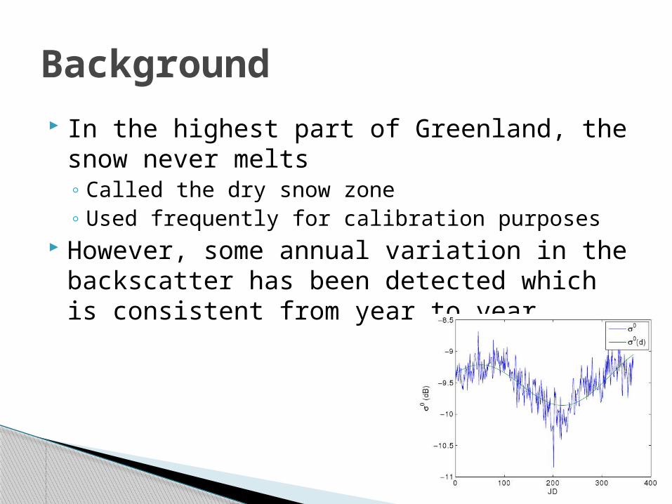
In the highest part of Greenland, the snow never melts◦ Called the dry snow zone◦ Used frequently for calibration purposes
However, some annual variation in the backscatter has been detected which is consistent from year to year
Background
This variation cannot be caused by melt because it does not drop below a specific threshold◦ Temperatures are typically between
However, it is possible that increasing temperatures do change the permittivity of the snow, thus changing the backscatter
Annual variation

We decided to test if received backscatter values could predict changes in permittivity
The answer to this would provide insight into possible causes for the annual variation◦ If backscatter cannot predict changes in
permittivity, then it is likely there are other factors affecting the annual variation
Problem

We created a model relating permittivity to backscatter (at least for snow)
Because knowing the temperature helps us predict the permittivity more accurately, we found a relationship between temperature and permittivity◦ This model required an intermediate step relating
temperature to snow density and snow density to permittivity
Theoretical Model
The equations for our model were (temperature to density)
(this is approximately linear)
(density to permittivity)
really complicated (several lines of equations)
Theoretical Model

Theoretical Results
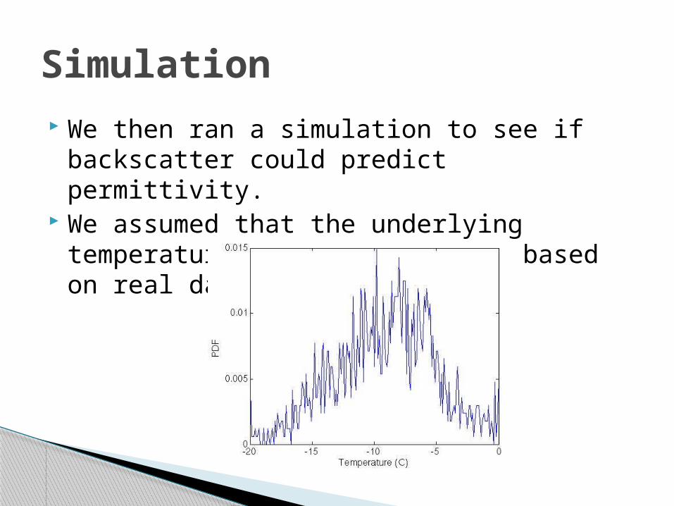
We then ran a simulation to see if backscatter could predict permittivity.
We assumed that the underlying temperature data was weighted based on real data
Simulation
Randomly generated temperatures using the histogram◦ Normalized the histogram◦ Calculated the cumulative distribution function◦ Generated uniformly distributed random numbers
between 0 and 1◦ Assigned each random number the temperature
value corresponding to the same index as the closest value of the cdf that was still less than the random number
Simulation

For a given temperature, the snow density, permittivity, and corresponding backscatter were calculated using the earlier equations
The backscatter was then corrupted with additive white Gaussian noise◦ This simulated real noise between the ground and
the satellite receiver, including atmospheric and instrumental noise
Simulation
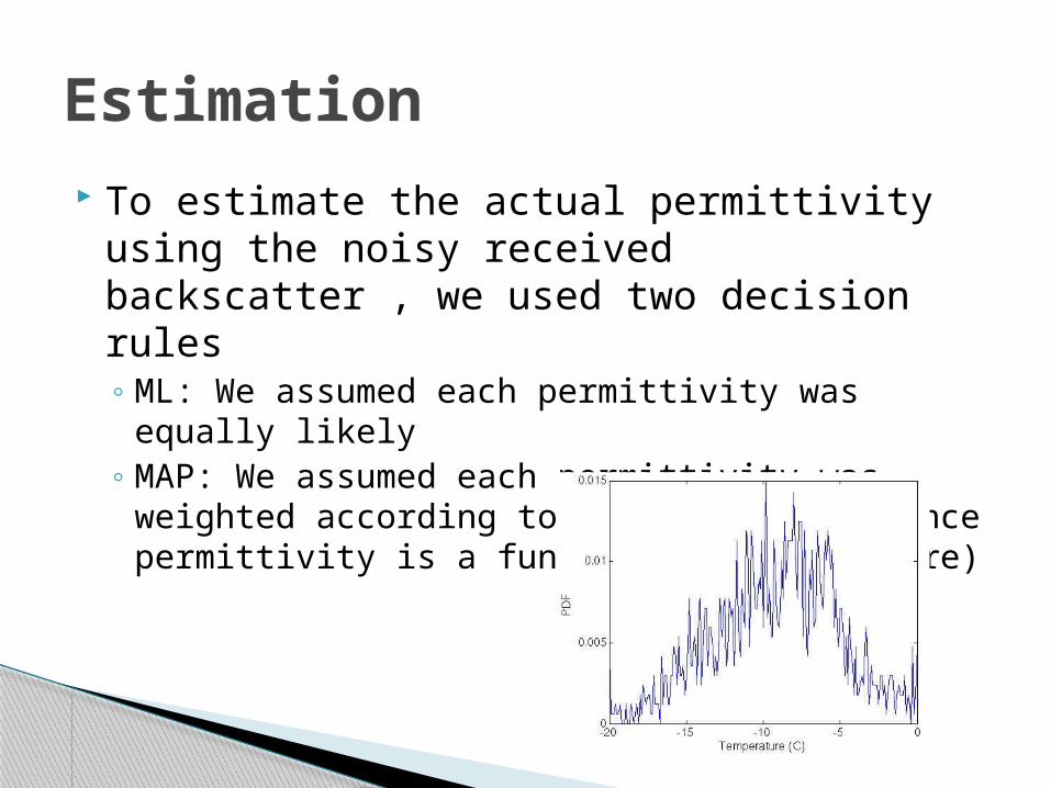
To estimate the actual permittivity using the noisy received backscatter , we used two decision rules◦ ML: We assumed each permittivity was equally
likely◦ MAP: We assumed each permittivity was weighted
according to the histogram (since permittivity is a function of temperature)
Estimation
The maximum likelihood rule is
That is, we choose the value of permittivity which makes receiving most likely.
Since is a function of permittivity, this is equivalent to
Maximum Likelihood (ML)
The goal is to choose , because that will give us the correct permittivity
Note that , where is a Gaussian random variable with 0 mean and variance related to SNR (white noise)
Hence, ◦ This is a Gaussian random variable
Maximum Likelihood
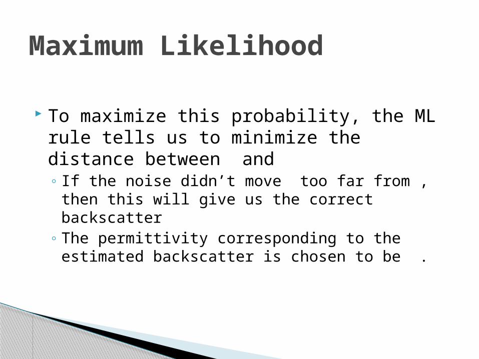
To maximize this probability, the ML rule tells us to minimize the distance between and ◦ If the noise didn’t move too far from , then this
will give us the correct backscatter◦ The permittivity corresponding to the estimated
backscatter is chosen to be .
Maximum Likelihood

The maximum a-posteriori rule is
We no longer assume that every permittivity is equally likely
This makes more sense given the distribution of temperatures
Maximum a-posteriori (MAP)
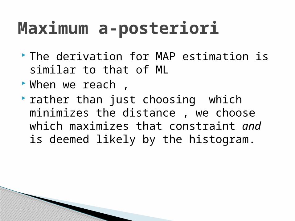
The derivation for MAP estimation is similar to that of ML
When we reach , rather than just choosing which minimizes
the distance , we choose which maximizes that constraint and is deemed likely by the histogram.
Maximum a-posteriori

MAP vs ML example
(or equivalently, permittivity or backscatter)
True value
Received value
What ML would estimate (minimize distance from received)
What MAP would estimate (this value is a lot more likely, even if the distance from received is further)
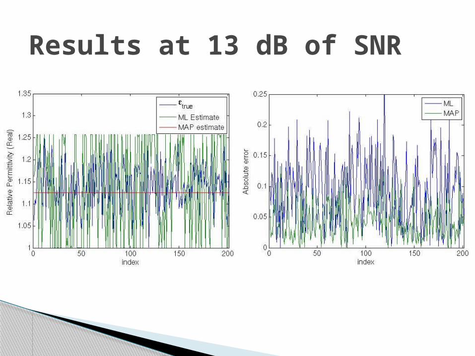
Results at 13 dB of SNR

MAP has superior performance to ML because there is more information available
However, neither estimator is a good predictor of permittivity based on received backscatter values
It is likely that the annual variation noticed in Greenland is caused by more than just changes in permittivity
Conclusions
Recommended