Kinetic equationsfrom stochastic dynamics in continuum
Yuri Kondratiev
Bielefeld University
Yuri Kondratiev (Bielefeld) Kinetic equations from stochastic dynamics in continuum 1 / 45
Setup
MACRO, MESO, and MICRO
Non-linear PDE and SPDE
as phenomenological models of complex systems.
Reaction-diffusion equations (RDE)
∂u
∂t= 4u+ f(u), u = u(t, x)
in combustion theory, bacterial growth, nerve propagation, epidemiology, geneticsetc.
RDE = Allen-Cahn = Ginzburg-Landau
Fisher equation: f(s) = s(1− s).
Yuri Kondratiev (Bielefeld) Kinetic equations from stochastic dynamics in continuum 2 / 45
Setup
We observe an active recent development in the study ofnon-local versions of RDE:
∂u
∂t= J ? u− u+ f(u), u = u(t, x).
u(0, x) = ϕ(x), x ∈ Ω ⊆ Rd
0 ≤ J ∈ L1, ‖J‖1 = 1 jump kernel.
Just few references:Coville, Dupaigne (2008)Ignat, Rossi (2010)Berestycki, Nadin, Ryzhik (2009)Pan, Li, Lin (2009)Zhang, Li, Sun (2010)
Yuri Kondratiev (Bielefeld) Kinetic equations from stochastic dynamics in continuum 3 / 45
Setup
Actually, such kind of equation was introduced byKolmogorov, Petrovsky and Piskunov (KPP) in 1937 (!)as a way to derive Fisher equation.
Local RDE (macroscopic description)are approximations tonon-local RDE (mesoscopic description)
Yuri Kondratiev (Bielefeld) Kinetic equations from stochastic dynamics in continuum 4 / 45
Setup
MACRO, MESO, and MICRO
Problem: derivation of meso- and macroscopic equations(deterministic or stochastic)from microscopic models .
There are known different techniques:– scaling limits for dynamics (hydrodynamic, Vlasov, Landau etc.)
– scaling of fluctuations (equilibrium or non-equilibrium)
– closure of (infinite linear) moment systems
– hierarchical chains (BBGKY etc.)
– particle approximation method
Yuri Kondratiev (Bielefeld) Kinetic equations from stochastic dynamics in continuum 5 / 45
Setup
Three levels in physics
In context of the theory of classical gases:
(Mi) is the level of particle dynamics (Newtons laws)
(Me) is the level of Boltzmann description
(Ma) is the level of continuum description.
Yuri Kondratiev (Bielefeld) Kinetic equations from stochastic dynamics in continuum 6 / 45
Setup
Microscopic Stochastic Systems
In mathematical terms we are interested in the links between the followingmathematical structures:
(Mi) the micro–scale of stochastically interacting entities (cells, individuals,. . .),in terms of (linear) Markov semigroups (or corresponding processes)
(Me) the meso–scale of statistical entities, in terms of continuous nonlinearsemigroups related to the solutions of nonlinear Boltzmann–type non-local kineticequations
(Ma) the macro–scale of densities of interacting entities (in terms of dynamicalsystems related to reaction–diffusion type equations).
Yuri Kondratiev (Bielefeld) Kinetic equations from stochastic dynamics in continuum 7 / 45
Setup General facts
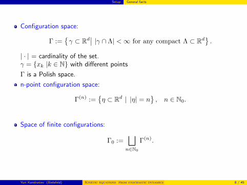
Configuration space:
Γ :=γ ⊂ Rd
∣∣ |γ ∩ Λ| <∞ for any compact Λ ⊂ Rd.
| · | = cardinality of the set.γ = xk |k ∈ N with different points
Γ is a Polish space.
n-point configuration space:
Γ(n) :=η ⊂ Rd | |η| = n
, n ∈ N0.
Space of finite configurations:
Γ0 :=⊔n∈N0
Γ(n).
Yuri Kondratiev (Bielefeld) Kinetic equations from stochastic dynamics in continuum 8 / 45
Setup General facts
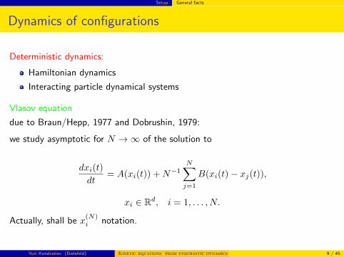
Dynamics of configurations
Deterministic dynamics:
Hamiltonian dynamics
Interacting particle dynamical systems
Vlasov equation
due to Braun/Hepp, 1977 and Dobrushin, 1979:
we study asymptotic for N →∞ of the solution to
dxi(t)
dt= A(xi(t)) +N−1
N∑j=1
B(xi(t)− xj(t)),
xi ∈ Rd, i = 1, . . . , N.
Actually, shall be x(N)i notation.
Yuri Kondratiev (Bielefeld) Kinetic equations from stochastic dynamics in continuum 9 / 45
Setup General facts
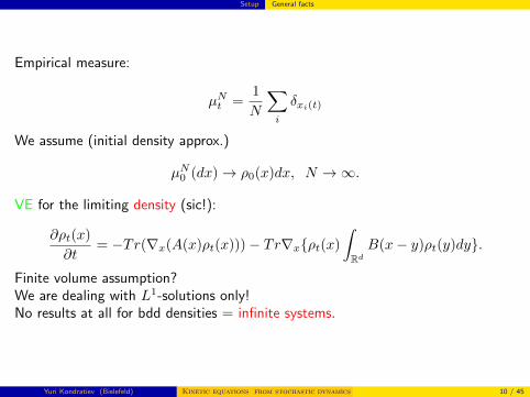
Empirical measure:
µNt =1
N
∑i
δxi(t)
We assume (initial density approx.)
µN0 (dx)→ ρ0(x)dx, N →∞.
VE for the limiting density (sic!):
∂ρt(x)
∂t= −Tr(∇x(A(x)ρt(x)))− Tr∇xρt(x)
∫RdB(x− y)ρt(y)dy.
Finite volume assumption?We are dealing with L1-solutions only!No results at all for bdd densities = infinite systems.
Yuri Kondratiev (Bielefeld) Kinetic equations from stochastic dynamics in continuum 10 / 45
Setup General facts
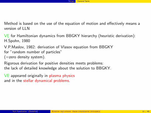
Method is based on the use of the equation of motion and effectively means aversion of LLN
VE for Hamiltonian dynamics from BBGKY hierarchy (heuristic derivation):H.Spohn, 1980
V.P.Maslov, 1982: derivation of Vlasov equation from BBGKYfor ”random number of particles”(=zero density system).
Rigorous derivation for positive densities meets problems:the lack of detailed knowledge about the solution to BBGKY.
VE appeared originally in plasma physicsand in the stellar dynamical problems.
Yuri Kondratiev (Bielefeld) Kinetic equations from stochastic dynamics in continuum 11 / 45
Setup General facts
Markov evolutions in continuum:
Diffusions (e.g., gradient diffusion)
Jumping particles Markov processes (e.g., Kawasaki dynamics)
Birth-and-death stochastic dynamics (e.g., Glauber, IBM in spatial ecology)
other stochastic IPS in Rd
Questions:
What is possible concept of related Vlasov equations?
May we work with infinite particle dynamics?
Is there a notion of a limiting IPS dynamics which creates Vlasov equation?
Other scalings and other kinetic equations?
Yuri Kondratiev (Bielefeld) Kinetic equations from stochastic dynamics in continuum 12 / 45
Setup General facts
Lattice framework: kinetic equations from lattice stochastic dynamics
For lattice stochastic dynamics and their hydrodynamic scalings
we have several excellent results by
Lebowitz, Presutti, Varadhan, Yau, Kipnis, Landimand many other authors
showing how macroscopic kinetic equations appear from microscopic stochasticprocesses.
Particular examples of non-local RDE were derived from lattice stochasticdynamics by Durrett, 1995.
Front propagation in these mesoscopic models analyzed by Perthame/Souganidis,2005.
Scaling of lattice stochastic dynamics to super-processes etc.
Yuri Kondratiev (Bielefeld) Kinetic equations from stochastic dynamics in continuum 13 / 45
Setup General facts
Our approach is based on the study of state evolutionfor the considered systems.
Markov dynamics of IPS ⇒ evolution of states (measures)
Particular scalings ⇒ different kinds of kinetic equations
General discussion for Hamiltonian dynamics:[Dobrushin/Sinai/Suhov], 1985.
Interacting diffusions:McKean-Vlasov limitwhich is a stochastic versionof the deterministic case.Classical results by McKean, Dawson, Gartner, Shiga et. al.
Yuri Kondratiev (Bielefeld) Kinetic equations from stochastic dynamics in continuum 14 / 45
General scheme of Vlasov scaling
Markov evolutions
Let L be a Markov pre-generator defined on some set of functions F(Γ)given on the configuration space Γ.
(Backward) Kolmogorov equation:
∂Ft∂t
= LFt,
Ft|t=0 = F0;
Duality: < F, µ >:=∫
ΓFdµ
(Forward) Kolmogorov = Fokker- Planck equation:
∂µt∂t
= L∗µt,
µt|t=0 = µ0.
Yuri Kondratiev (Bielefeld) Kinetic equations from stochastic dynamics in continuum 15 / 45
General scheme of Vlasov scaling
Vlasov scaling
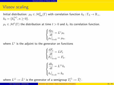
Initial distribution: µ0 ∈M1fm(Γ) with correlation function k0 : Γ0 → R+,
k0 = k(n)0 , n ≥ 0.
µt ∈M1(Γ) the distribution at time t > 0 and kt its correlation function.dµtdt
= L∗µt
µt∣∣t=0
= µ0,
where L∗ is the adjoint to the generator on functionsdFtdt
= LFt
Ft∣∣t=0
= F0.dktdt
= L4kt
kt∣∣t=0
= k0
where L4 := L∗ is the generator of a semigroup T4t := T ∗t .Yuri Kondratiev (Bielefeld) Kinetic equations from stochastic dynamics in continuum 16 / 45
General scheme of Vlasov scaling
1st step in VS
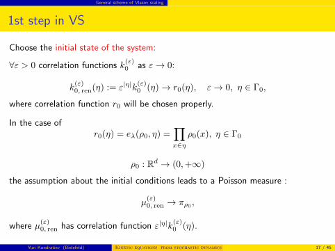
Choose the initial state of the system:
∀ε > 0 correlation functions k(ε)0 as ε→ 0:
k(ε)0, ren(η) := ε|η|k
(ε)0 (η)→ r0(η), ε→ 0, η ∈ Γ0,
where correlation function r0 will be chosen properly.
In the case ofr0(η) = eλ(ρ0, η) =
∏x∈η
ρ0(x), η ∈ Γ0
ρ0 : Rd → (0,+∞)
the assumption about the initial conditions leads to a Poisson measure :
µ(ε)0, ren → πρ0 ,
where µ(ε)0, ren has correlation function ε|η|k
(ε)0 (η).
Yuri Kondratiev (Bielefeld) Kinetic equations from stochastic dynamics in continuum 17 / 45
General scheme of Vlasov scaling
2nd step in VS
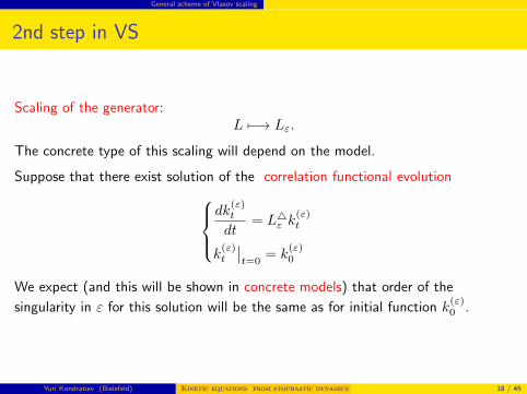
Scaling of the generator:L 7−→ Lε.
The concrete type of this scaling will depend on the model.
Suppose that there exist solution of the correlation functional evolutiondk
(ε)t
dt= L4ε k
(ε)t
k(ε)t
∣∣t=0
= k(ε)0
We expect (and this will be shown in concrete models) that order of the
singularity in ε for this solution will be the same as for initial function k(ε)0 .
Yuri Kondratiev (Bielefeld) Kinetic equations from stochastic dynamics in continuum 18 / 45
General scheme of Vlasov scaling
3rd step in VS
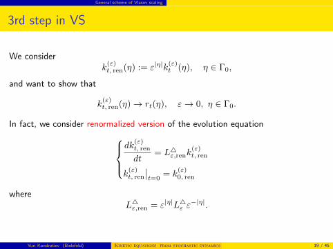
We considerk
(ε)t, ren(η) := ε|η|k
(ε)t (η), η ∈ Γ0,
and want to show that
k(ε)t, ren(η)→ rt(η), ε→ 0, η ∈ Γ0.
In fact, we consider renormalized version of the evolution equationdk
(ε)t, ren
dt= L4ε,renk
(ε)t, ren
k(ε)t, ren
∣∣t=0
= k(ε)0, ren
whereL4ε,ren = ε|η|L4ε ε
−|η|.
Yuri Kondratiev (Bielefeld) Kinetic equations from stochastic dynamics in continuum 19 / 45
General scheme of Vlasov scaling
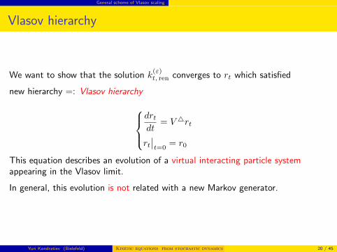
Vlasov hierarchy
We want to show that the solution k(ε)t, ren converges to rt which satisfied
new hierarchy =: Vlasov hierarchy
drtdt
= V 4rt
rt∣∣t=0
= r0
This equation describes an evolution of a virtual interacting particle systemappearing in the Vlasov limit.
In general, this evolution is not related with a new Markov generator.
Yuri Kondratiev (Bielefeld) Kinetic equations from stochastic dynamics in continuum 20 / 45
General scheme of Vlasov scaling
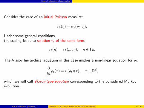
Consider the case of an initial Poisson measure:
r0(η) = eλ(ρ0, η).
Under some general conditions,the scaling leads to solution rt of the same form:
rt(η) = eλ(ρt, η), η ∈ Γ0.
The Vlasov hierarchical equation in this case implies a non-linear equation for ρt:
∂
∂tρt(x) = υ(ρt)(x), x ∈ Rd,
which we will call Vlasov-type equation corresponding to the considered Markovevolution.
Yuri Kondratiev (Bielefeld) Kinetic equations from stochastic dynamics in continuum 21 / 45
Derivation of Vlasov hierarchies
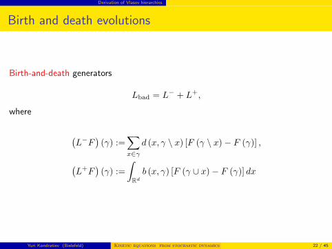
Birth and death evolutions
Birth-and-death generators
Lbad = L− + L+,
where
(L−F
)(γ) :=
∑x∈γ
d (x, γ \ x) [F (γ \ x)− F (γ)] ,
(L+F
)(γ) :=
∫Rdb (x, γ) [F (γ ∪ x)− F (γ)] dx
Yuri Kondratiev (Bielefeld) Kinetic equations from stochastic dynamics in continuum 22 / 45
Derivation of Vlasov hierarchies
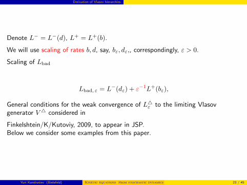
Denote L− = L−(d), L+ = L+(b).
We will use scaling of rates b, d, say, bε, dε,, correspondingly, ε > 0.
Scaling of Lbad
Lbad, ε = L−(dε) + ε−1L+(bε),
General conditions for the weak convergence of L4ε to the limiting Vlasovgenerator V 4 considered in
Finkelshtein/K/Kutoviy, 2009, to appear in JSP.Below we consider some examples from this paper.
Yuri Kondratiev (Bielefeld) Kinetic equations from stochastic dynamics in continuum 23 / 45
Derivation of Vlasov hierarchies Particular models: B-A-D systems
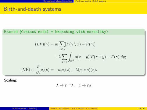
Birth-and-death systems
Example (Contact model = branching with mortality)
(LF )(γ) = m∑x∈γ
[F (γ \ x)− F (γ)]
+ λ∑x∈γ
∫Rda(x− y)[F (γ ∪ y)− F (γ)]dy;
(VE) :∂
∂tρt(x) = −mρt(x) + λ(ρt ∗ a)(x).
Scaling:λ 7→ ε−1λ, a 7→ εa
Yuri Kondratiev (Bielefeld) Kinetic equations from stochastic dynamics in continuum 24 / 45
Derivation of Vlasov hierarchies Particular models: B-A-D systems
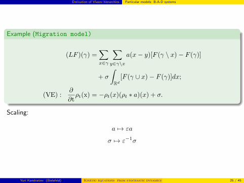
Example (Migration model)
(LF )(γ) =∑x∈γ
∑y∈γ\x
a(x− y)[F (γ \ x)− F (γ)]
+ σ
∫Rd
[F (γ ∪ x)− F (γ)]dx;
(VE) :∂
∂tρt(x) = −ρt(x)(ρt ∗ a)(x) + σ.
Scaling:
a 7→ εa
σ 7→ ε−1σ
Yuri Kondratiev (Bielefeld) Kinetic equations from stochastic dynamics in continuum 25 / 45
Derivation of Vlasov hierarchies Particular models: B-A-D systems
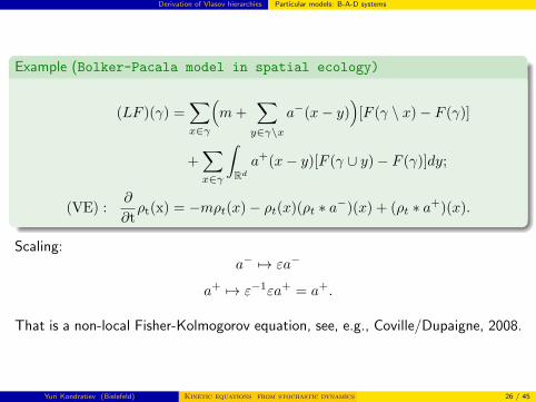
Example (Bolker-Pacala model in spatial ecology)
(LF )(γ) =∑x∈γ
(m+
∑y∈γ\x
a−(x− y))
[F (γ \ x)− F (γ)]
+∑x∈γ
∫Rda+(x− y)[F (γ ∪ y)− F (γ)]dy;
(VE) :∂
∂tρt(x) = −mρt(x)− ρt(x)(ρt ∗ a−)(x) + (ρt ∗ a+)(x).
Scaling:a− 7→ εa−
a+ 7→ ε−1εa+ = a+.
That is a non-local Fisher-Kolmogorov equation, see, e.g., Coville/Dupaigne, 2008.
Yuri Kondratiev (Bielefeld) Kinetic equations from stochastic dynamics in continuum 26 / 45
Derivation of Vlasov hierarchies Particular models: B-A-D systems
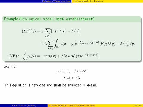
Example (Ecological model with establishment)
(LF )(γ) = m∑x∈γ
[F (γ \ x)− F (γ)]
+ λ∑x∈γ
∫Rda(x− y)e−
∑u∈γ φ(y−u)[F (γ ∪ y)− F (γ)]dy;
(VE) :∂
∂tρt(x) = −mρt(x) + λ(a ∗ ρt)(x)e−(φ∗ρt)(x).
Scaling:a 7→ εa, φ 7→ εφ
λ 7→ ε−1λ
This equation is new one and shall be analyzed in detail.
Yuri Kondratiev (Bielefeld) Kinetic equations from stochastic dynamics in continuum 27 / 45
Derivation of Vlasov hierarchies Particular models: B-A-D systems
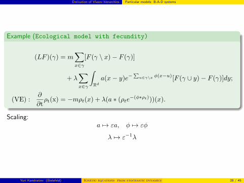
Example (Ecological model with fecundity)
(LF )(γ) = m∑x∈γ
[F (γ \ x)− F (γ)]
+ λ∑x∈γ
∫Rda(x− y)e−
∑u∈γ\x φ(x−u)[F (γ ∪ y)− F (γ)]dy;
(VE) :∂
∂tρt(x) = −mρt(x) + λ(a ∗ (ρte
−(φ∗ρt)))(x).
Scaling:a 7→ εa, φ 7→ εφ
λ 7→ ε−1λ
Yuri Kondratiev (Bielefeld) Kinetic equations from stochastic dynamics in continuum 28 / 45
Derivation of Vlasov hierarchies Particular models: B-A-D systems
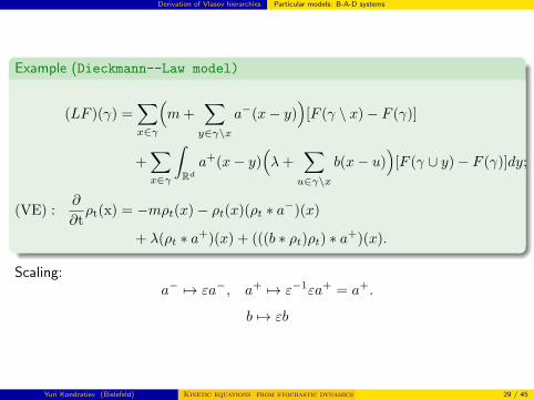
Example (Dieckmann--Law model)
(LF )(γ) =∑x∈γ
(m+
∑y∈γ\x
a−(x− y))
[F (γ \ x)− F (γ)]
+∑x∈γ
∫Rda+(x− y)
(λ+
∑u∈γ\x
b(x− u))
[F (γ ∪ y)− F (γ)]dy;
(VE) :∂
∂tρt(x) = −mρt(x)− ρt(x)(ρt ∗ a−)(x)
+ λ(ρt ∗ a+)(x) + (((b ∗ ρt)ρt) ∗ a+)(x).
Scaling:a− 7→ εa−, a+ 7→ ε−1εa+ = a+.
b 7→ εb
Yuri Kondratiev (Bielefeld) Kinetic equations from stochastic dynamics in continuum 29 / 45
Derivation of Vlasov hierarchies Particular models: conservative particle systems
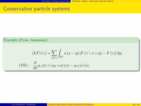
Conservative particle systems
Example (Free Kawasaki)
(LF ) (γ) =∑x∈γ
∫Rda (x− y) [F (γ \ x ∪ y)− F (γ)] dy;
(VE) :∂
∂tρt (x) = (ρt ∗ a) (x)− ρt (x) 〈a〉 .
Yuri Kondratiev (Bielefeld) Kinetic equations from stochastic dynamics in continuum 30 / 45
Derivation of Vlasov hierarchies Particular models: conservative particle systems
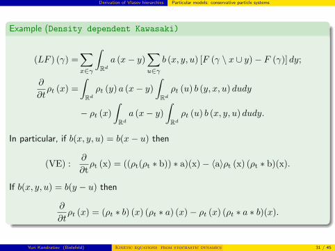
Example (Density dependent Kawasaki)
(LF ) (γ) =∑x∈γ
∫Rda (x− y)
∑u∈γ
b (x, y, u) [F (γ \ x ∪ y)− F (γ)] dy;
∂
∂tρt (x) =
∫Rdρt (y) a (x− y)
∫Rdρt (u) b (y, x, u) dudy
− ρt (x)
∫Rda (x− y)
∫Rdρt (u) b (x, y, u) dudy.
In particular, if b(x, y, u) = b(x− u) then
(VE) :∂
∂tρt (x) = ((ρt(ρt ∗ b)) ∗ a)(x)− 〈a〉ρt (x) (ρt ∗ b)(x).
If b(x, y, u) = b(y − u) then
∂
∂tρt (x) = (ρt ∗ b) (x) (ρt ∗ a) (x)− ρt (x) (ρt ∗ a ∗ b)(x).
Yuri Kondratiev (Bielefeld) Kinetic equations from stochastic dynamics in continuum 31 / 45
Derivation of Vlasov hierarchies Particular models: conservative particle systems
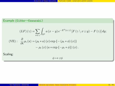
Example (Gibbs--Kawasaki)
(LF ) (γ) =∑x∈γ
∫Rda (x− y) e−E
φ(x,γ) [F (γ \ x ∪ y)− F (γ)] dy;
(VE) :∂
∂tρt (x) = (ρt ∗ a) (x) exp − (ρt ∗ φ) (x)
− ρt (x) (a ∗ exp −ρt ∗ φ) (x) .
Scaling:φ 7→ εφ
Yuri Kondratiev (Bielefeld) Kinetic equations from stochastic dynamics in continuum 32 / 45
Derivation of Vlasov hierarchies Particular models: conservative particle systems
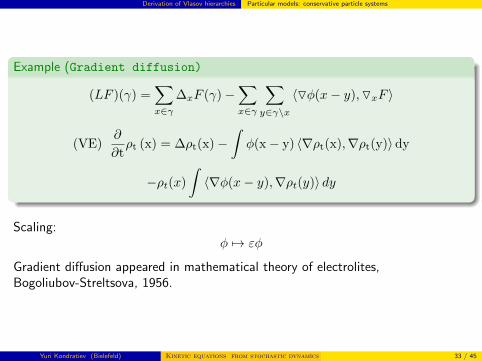
Example (Gradient diffusion)
(LF )(γ) =∑x∈γ
∆xF (γ)−∑x∈γ
∑y∈γ\x
〈Oφ(x− y),OxF 〉
(VE)∂
∂tρt (x) = ∆ρt(x)−
∫φ(x− y) 〈∇ρt(x),∇ρt(y)〉dy
−ρt(x)
∫〈∇φ(x− y),∇ρt(y)〉 dy
Scaling:φ 7→ εφ
Gradient diffusion appeared in mathematical theory of electrolites,Bogoliubov-Streltsova, 1956.
Yuri Kondratiev (Bielefeld) Kinetic equations from stochastic dynamics in continuum 33 / 45
Derivation of Vlasov hierarchies Particular models: conservative particle systems
Convergence problem
In all models above the weak convergence of the generators
L4ε → V 4, ε→ 0
is shown.
A difficult question: convergence of solutions of hierarchical equations to theVlasov hierarchy solution.
In each model even just the problem of the existence for the solution to hierarchyneed a special analysis and difficult technical work (non-equilibrium dynamics).
But we need essentially more:detailed control of the solution uniformly w.r.t. parameters on any finite timeinterval.
Two regimes:
zero density systems = L1 solutions to be considered
positive density systems = L∞ solutions
Yuri Kondratiev (Bielefeld) Kinetic equations from stochastic dynamics in continuum 34 / 45
Derivation of Vlasov hierarchies Particular models: conservative particle systems
For the positive density case only knownresults (Finkelshtein/K/Kutoviy 2009-2010) concern
Contact Model
Migration Model
Glauber Dynamics
Bolker-Pacala model in spatial ecology
Zero density case should be possible to analyze also in other modelsand under more relaxing conditions on parameters (work in progress).
Yuri Kondratiev (Bielefeld) Kinetic equations from stochastic dynamics in continuum 35 / 45
Inter-spices interactions in spatial ecology
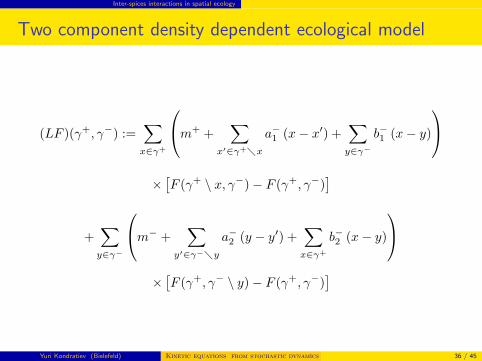
Two component density dependent ecological model
(LF )(γ+, γ−) :=∑x∈γ+
m+ +∑
x′∈γ+x
a−1 (x− x′) +∑y∈γ−
b−1 (x− y)
×[F (γ+ \ x, γ−)− F (γ+, γ−)
]
+∑y∈γ−
m− +∑
y′∈γ−y
a−2 (y − y′) +∑x∈γ+
b−2 (x− y)
×[F (γ+, γ− \ y)− F (γ+, γ−)
]
Yuri Kondratiev (Bielefeld) Kinetic equations from stochastic dynamics in continuum 36 / 45
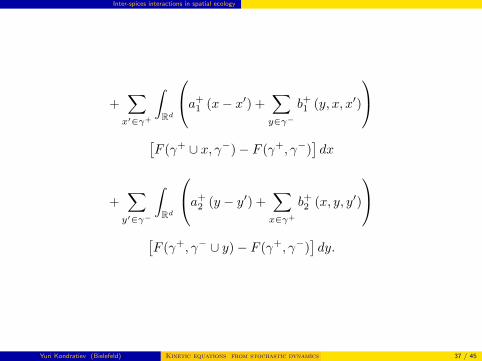
Inter-spices interactions in spatial ecology
+∑x′∈γ+
∫Rd
a+1 (x− x′) +
∑y∈γ−
b+1 (y, x, x′)
[F (γ+ ∪ x, γ−)− F (γ+, γ−)
]dx
+∑y′∈γ−
∫Rd
a+2 (y − y′) +
∑x∈γ+
b+2 (x, y, y′)
[F (γ+, γ− ∪ y)− F (γ+, γ−)
]dy.
Yuri Kondratiev (Bielefeld) Kinetic equations from stochastic dynamics in continuum 37 / 45
Inter-spices interactions in spatial ecology
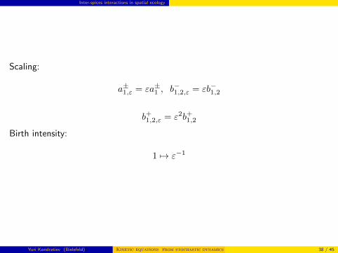
Scaling:
a±1,ε = εa±1 , b−1,2,ε = εb−1,2
b+1,2,ε = ε2b+1,2
Birth intensity:
1 7→ ε−1
Yuri Kondratiev (Bielefeld) Kinetic equations from stochastic dynamics in continuum 38 / 45
Inter-spices interactions in spatial ecology
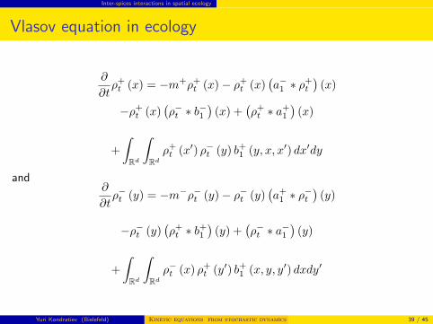
Vlasov equation in ecology
∂
∂tρ+t (x) = −m+ρ+
t (x)− ρ+t (x)
(a−1 ∗ ρ
+t
)(x)
−ρ+t (x)
(ρ−t ∗ b−1
)(x) +
(ρ+t ∗ a+
1
)(x)
+
∫Rd
∫Rdρ+t (x′) ρ−t (y) b+1 (y, x, x′) dx′dy
and∂
∂tρ−t (y) = −m−ρ−t (y)− ρ−t (y)
(a+
1 ∗ ρ−t
)(y)
−ρ−t (y)(ρ+t ∗ b+1
)(y) +
(ρ−t ∗ a−1
)(y)
+
∫Rd
∫Rdρ−t (x) ρ+
t (y′) b+1 (x, y, y′) dxdy′
Yuri Kondratiev (Bielefeld) Kinetic equations from stochastic dynamics in continuum 39 / 45
Hydrodynamic equations
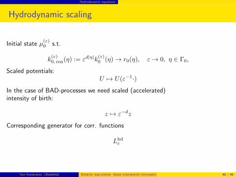
Hydrodynamic scaling
Initial state µ(ε)0 s.t.
k(ε)0, ren(η) := εd|η|k
(ε)0 (η)→ r0(η), ε→ 0, η ∈ Γ0,
Scaled potentials:U 7→ U(ε−1·)
In the case of BAD-processes we need scaled (accelerated)intensity of birth:
z 7→ ε−dz
Corresponding generator for corr. functions
Lhdε
Yuri Kondratiev (Bielefeld) Kinetic equations from stochastic dynamics in continuum 40 / 45
Hydrodynamic equations
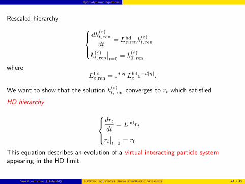
Rescaled hierarchy dk
(ε)t, ren
dt= Lhd
ε,renk(ε)t, ren
k(ε)t, ren
∣∣t=0
= k(ε)0, ren
whereLhdε,ren = εd|η|Lhd
ε ε−d|η|.
We want to show that the solution k(ε)t, ren converges to rt which satisfied
HD hierarchy
drtdt
= Lhdrt
rt∣∣t=0
= r0
This equation describes an evolution of a virtual interacting particle systemappearing in the HD limit.
Yuri Kondratiev (Bielefeld) Kinetic equations from stochastic dynamics in continuum 41 / 45
Hydrodynamic equations
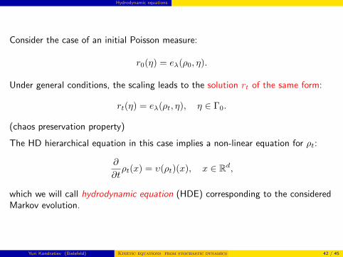
Consider the case of an initial Poisson measure:
r0(η) = eλ(ρ0, η).
Under general conditions, the scaling leads to the solution rt of the same form:
rt(η) = eλ(ρt, η), η ∈ Γ0.
(chaos preservation property)
The HD hierarchical equation in this case implies a non-linear equation for ρt:
∂
∂tρt(x) = υ(ρt)(x), x ∈ Rd,
which we will call hydrodynamic equation (HDE) corresponding to the consideredMarkov evolution.
Yuri Kondratiev (Bielefeld) Kinetic equations from stochastic dynamics in continuum 42 / 45
Hydrodynamic equations
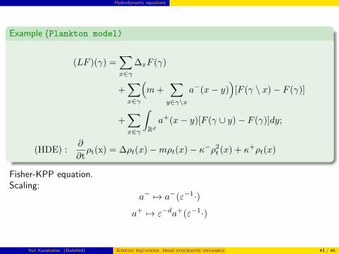
Example (Plankton model)
(LF )(γ) =∑x∈γ
∆xF (γ)
+∑x∈γ
(m+
∑y∈γ\x
a−(x− y))
[F (γ \ x)− F (γ)]
+∑x∈γ
∫Rda+(x− y)[F (γ ∪ y)− F (γ)]dy;
(HDE) :∂
∂tρt(x) = ∆ρt(x)−mρt(x)− κ−ρ2
t (x) + κ+ρt(x)
Fisher-KPP equation.Scaling:
a− 7→ a−(ε−1·)
a+ 7→ ε−da+(ε−1·)
Yuri Kondratiev (Bielefeld) Kinetic equations from stochastic dynamics in continuum 43 / 45
Mixed scaling for BAD dynamics
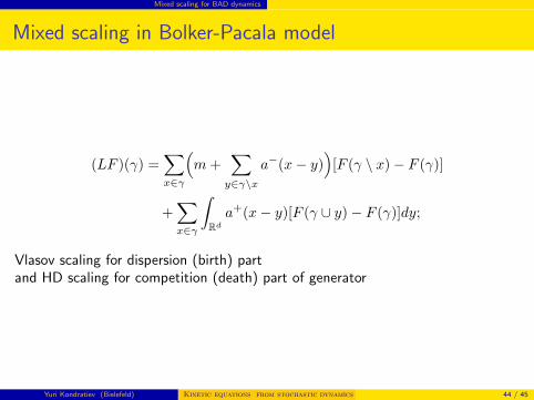
Mixed scaling in Bolker-Pacala model
(LF )(γ) =∑x∈γ
(m+
∑y∈γ\x
a−(x− y))
[F (γ \ x)− F (γ)]
+∑x∈γ
∫Rda+(x− y)[F (γ ∪ y)− F (γ)]dy;
Vlasov scaling for dispersion (birth) partand HD scaling for competition (death) part of generator
Yuri Kondratiev (Bielefeld) Kinetic equations from stochastic dynamics in continuum 44 / 45
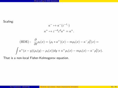
Mixed scaling for BAD dynamics
Scaling:a− 7→ a−(ε−1·)
a+ 7→ ε−dεda+ = a+.
(HDE) :∂
∂tρt(x) = (ρt ∗ a+)(x)−mρt(x)− κ−ρ2
t (x) =∫a+(x− y)(ρt(y)− ρt(x))dy + κ+ρt(x)−mρt(x)− κ−ρ2
t (x).
That is a non-local Fisher-Kolmogorov equation.
Yuri Kondratiev (Bielefeld) Kinetic equations from stochastic dynamics in continuum 45 / 45
Recommended


![A hybrid smoothed dissipative particle dynamics (SDPD ...the deterministic spatial dynamics but not the stochastic dynamics. The spatial stochastic simulation 80 algorithm (sSSA) [29]](https://img.pdfslide.net/doc/110x75/5f41a2ab66492703c57addfe/a-hybrid-smoothed-dissipative-particle-dynamics-sdpd-the-deterministic-spatial.jpg)