Introduction to ComputationalNeuroscienceLecture 4: Data analysis I
viernes, 16 de septiembre de 16
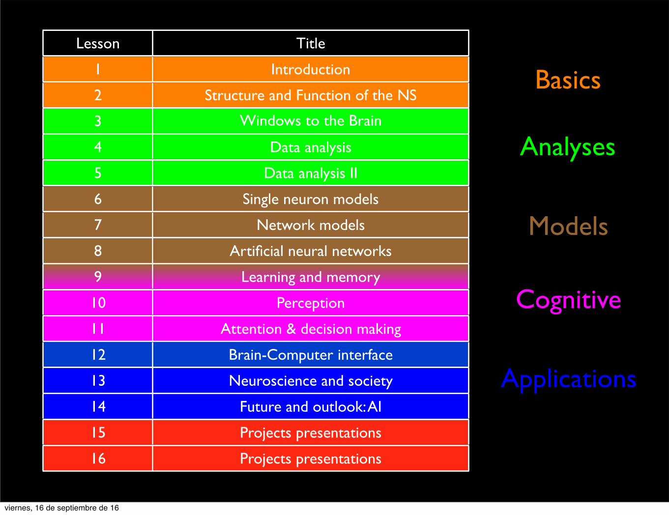
Applications
Cognitive
Models
Analyses
Basics
Lesson Title
1 Introduction
2 Structure and Function of the NS
3 Windows to the Brain
4 Data analysis
5 Data analysis II
6 Single neuron models
7 Network models
8 Artificial neural networks
9 Learning and memory
10 Perception
11 Attention & decision making
12 Brain-Computer interface
13 Neuroscience and society
14 Future and outlook: AI
15 Projects presentations
16 Projects presentations
viernes, 16 de septiembre de 16

http://www.psychology.ut.ee/en/about-us/location
http://www.psychology.ut.ee/en/about-us/laboratory-experimental-psychology
viernes, 16 de septiembre de 16
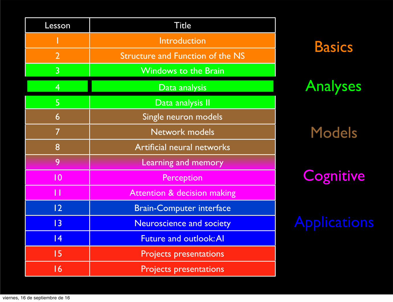
Neuroimaging
Structural brain imaging techniques are used to resolvethe anatomy of the brain in a living subject without physically penetrating the skull
Functional brain imaging techniques are used to measureneural activity without physically penetrating the skull
* Measure anatomical changes over time
* Diagnose diseases such as tumors or vascular disorders
* Which neural structures are active during certain mental operations?
viernes, 16 de septiembre de 16

Functional brain imaging
Non-invasive
recording from
human brain
(Functional
brain imaging)
Positron emission
tomography
(PET)
Functional magnetic
resonance imaging
(fMRI)
Electro-
encephalography
(EEG)
Magneto-
encephalography
(MEG)
Excellent spatial
resolution (~1-2mm)
Poor temporal
resolution (~1sec)
Poor spatial
resolution (esp. EEG)
Excellent temporal
resolution (<1msec)
Hemodynamic
techniques
Electro-magnetic
techniques
viernes, 16 de septiembre de 16

Extracellular recordings
Easier than intracellular in vivo
Requires spike sorting to identify which cell fire which a.p.
107Chapter | 4 Electrophysiology
single unit data to be obtained by recording multiple cells at once. Identifying individual cells based on their spiking activity and assigning the waveforms to particular cells is known as spike sorting .
By investigating the activity of dozens of neurons at a time, it is possible to answer questions regarding connectivity and timing within a neural network. A scientist can also manipulate specific neurons within the network and monitor the effect on other neurons recorded by the array. Ultimately, using MEAs to study the simultaneous response of neural circuits provides pivotal information on neuronal interactions, as well as spatiotemporal information about neural networks.
MEAs can be used to record from multiple neurons in vitro or in vivo. In vitro , a brain slice can be placed over a grid of many microelectrodes for extra-cellular recordings. In vivo tetrodes or MEAs can be implanted in the intact brains of live animals for multiunit recordings. Multielectrode technology has also been used in non-human primates for long-term recording. For example, network activity recorded using MEAs in the premotor cortex of monkeys while they perform reaching tasks is being studied to develop neural prosthetics that would allow animals (including humans) to move a prosthetic device using conscious thought.
Intracellular Recording
While extracellular recordings detect action potentials, intracellular recordings detect the small, graded changes in local membrane potential caused by syn-aptic events. Intracellular recording requires impaling a neuron or axon with a
Tetrode Multielectrode Array
Electrodes
Guide tube
Plug
A B
Electrodes
Base
FIGURE 4.6 Two specialized types of electrodes for recording from more than one neuron. (A) A tetrode is composed of four microelectrode wires rolled into a single device. A scientist implants a tetrode into the brain of an animal and connects the top plug to a cable attached to the amplifier. (B) A microelectrode array is composed of 25 or more electrodes (sometimes over 100) and is used to record from neurons on the surface of the brain. Multielectrode arrays can also be used to record from slices in vitro .
Records a few tens up to hundreds neurons
viernes, 16 de septiembre de 16
Summary
• Structural (functional) brain imaging capture the anatomy (activation) of different brain regions
• MRI (fMRI) technique of choice for good spatial resolution
• EEG and MEG have excellent temporal resolution
• Electrophysiology techniques measure activity at the neuron level
• No perfect technique allows yet to monitor extensive regions of brain circuits with a single-neuron resolution
viernes, 16 de septiembre de 16

Analysis is what lies between data and results
viernes, 16 de septiembre de 16
Learning objectives
• Understand the basic analyses for continuous and spiking electrophysiology data
viernes, 16 de septiembre de 16

Continuous signals
Spikes
viernes, 16 de septiembre de 16
Event Related Potentials (ERPs)
Analysis of rhythmic data (power spectrum)
Association measures (networks)
Continuous signals
viernes, 16 de septiembre de 16

Event Related Potential
http://neurocog.psy.tufts.edu/images/ERP_technique.gif
In many experiments we are interested in the activity generated by some event... (ex., sensory stimulus or behavior)
viernes, 16 de septiembre de 16
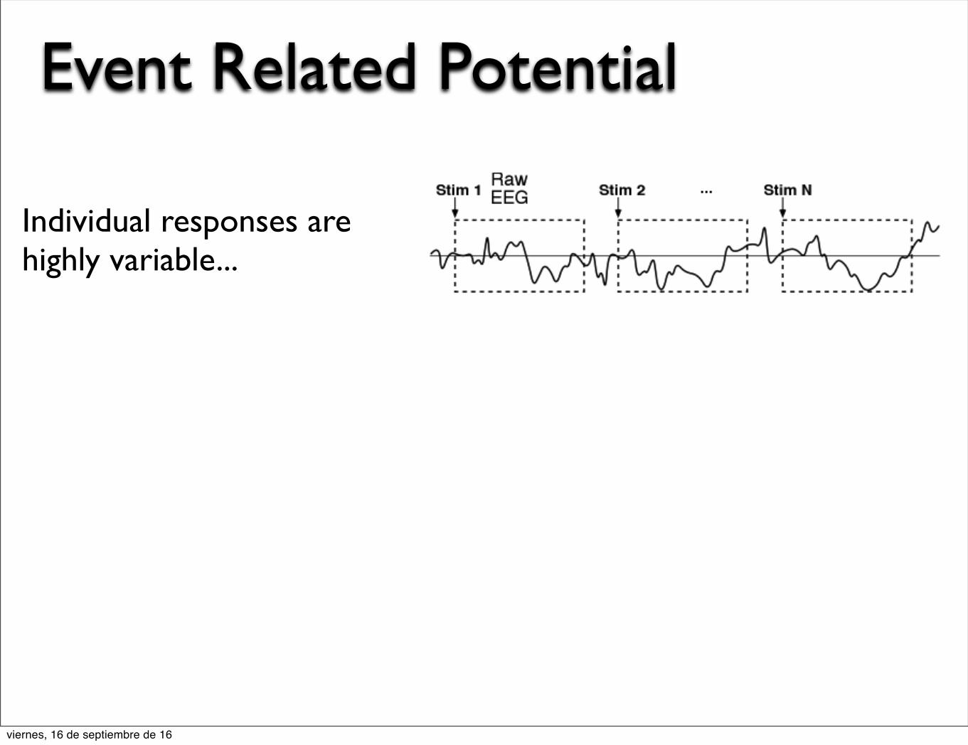
Event Related Potential
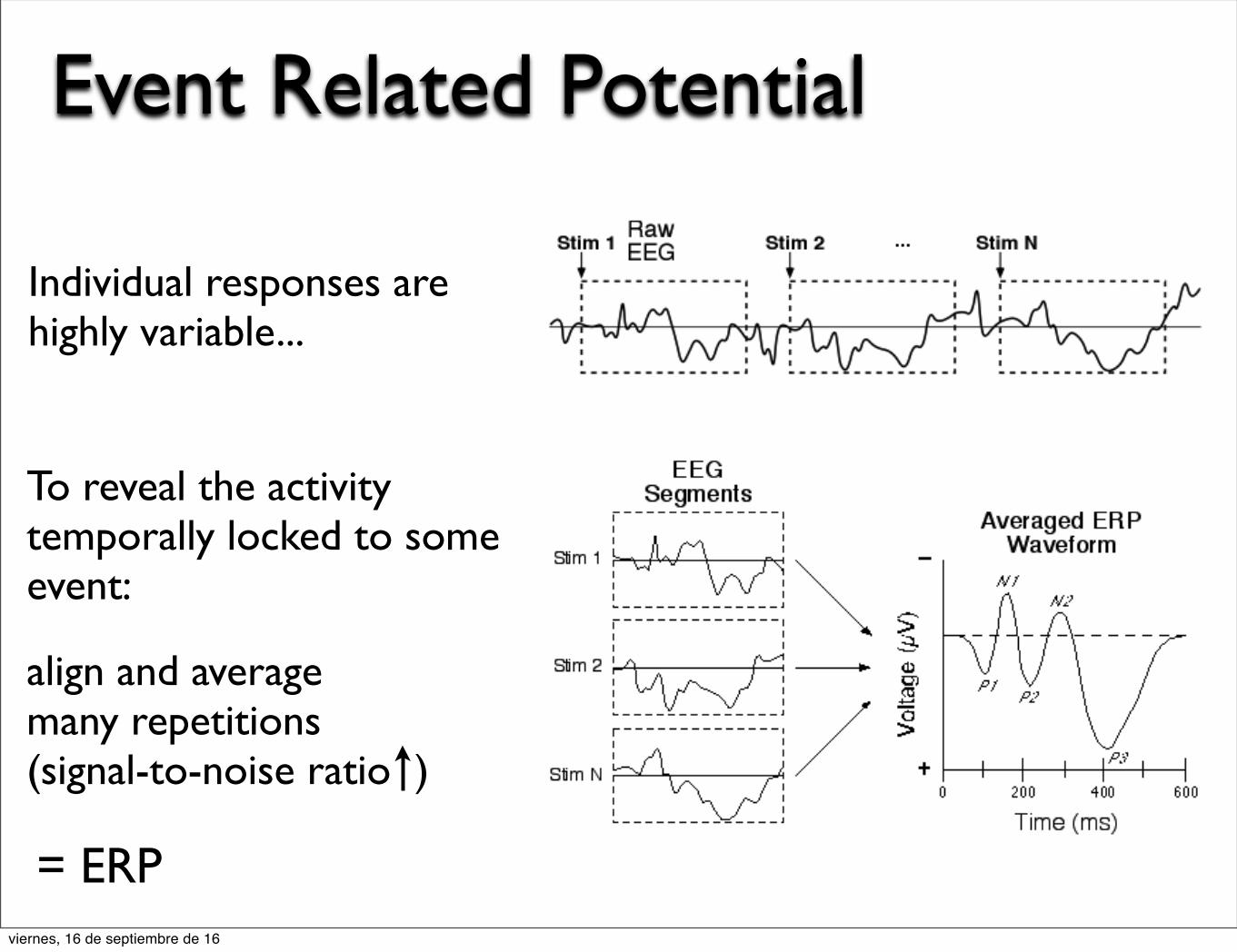
Individual responses arehighly variable...
viernes, 16 de septiembre de 16
Event Related Potential
Individual responses arehighly variable...
To reveal the activity temporally locked to some event:
align and average many repetitions(signal-to-noise ratio )
= ERPviernes, 16 de septiembre de 16

ERP (nomenclature)
http://neurocog.psy.tufts.edu/images/ERP_components.gif
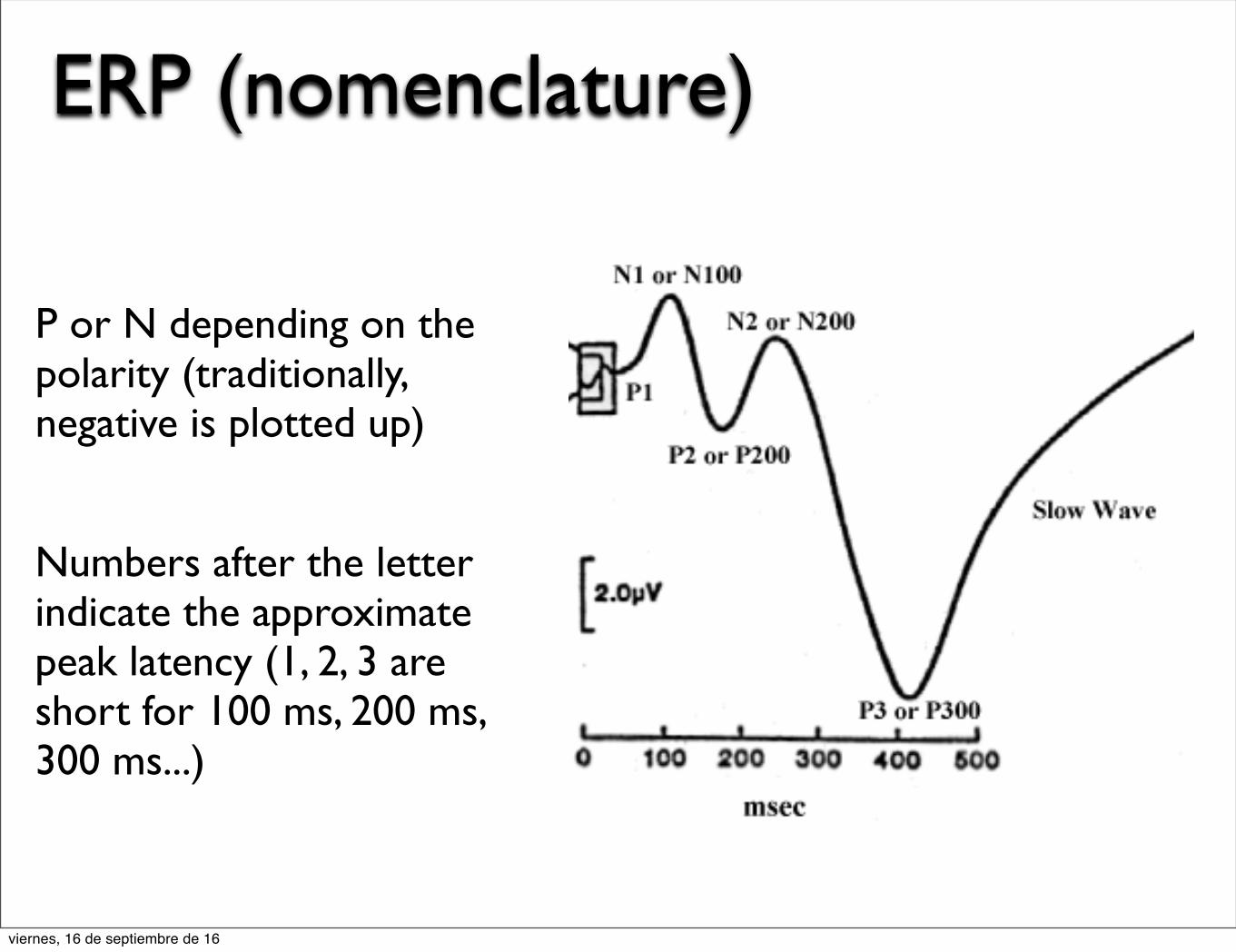
Labelling of ERP components(warning: a bit confusing)
P or N: whether thecomponent is negative orpositive going.
Number after the letter:indicates the approximatepeak latency of thecomponents. 1, 2, 3, etc.are short for 100ms,200ms, 300ms and soforth.
Traditionally, negative isplotted up and positivedown.
viernes, 16 de septiembre de 16
ERP (nomenclature)
http://neurocog.psy.tufts.edu/images/ERP_components.gif
Labelling of ERP components(warning: a bit confusing)
P or N: whether thecomponent is negative orpositive going.
Number after the letter:indicates the approximatepeak latency of thecomponents. 1, 2, 3, etc.are short for 100ms,200ms, 300ms and soforth.
Traditionally, negative isplotted up and positivedown.
P or N depending on the polarity (traditionally, negative is plotted up)
Numbers after the letterindicate the approximatepeak latency (1, 2, 3 are short for 100 ms, 200 ms,300 ms...)
viernes, 16 de septiembre de 16
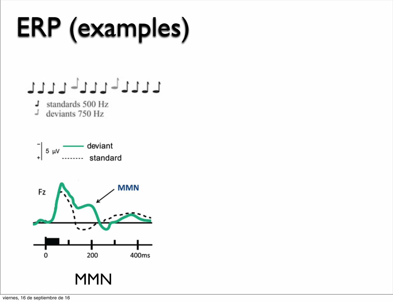
ERP (examples)
MMNviernes, 16 de septiembre de 16

ERP (examples)
MMN P300viernes, 16 de septiembre de 16
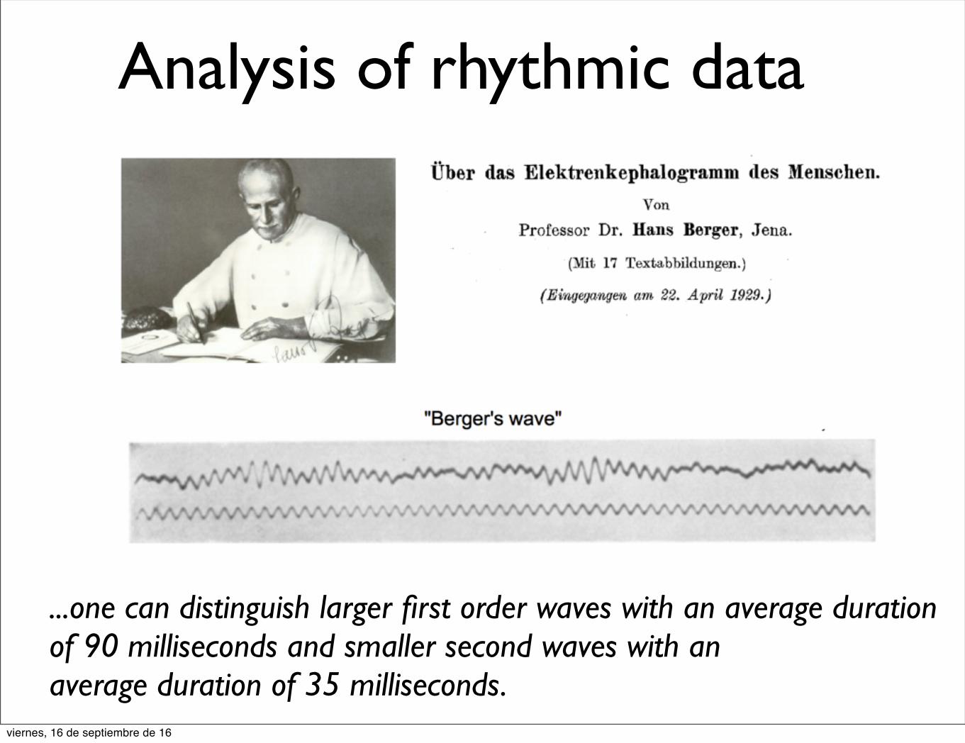
Analysis of rhythmic data
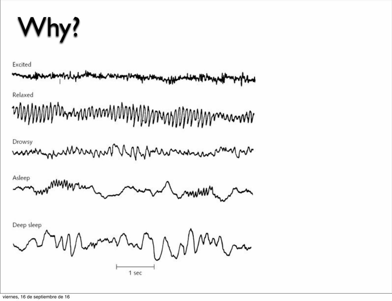
...one can distinguish larger first order waves with an average duration of 90 milliseconds and smaller second waves with an average duration of 35 milliseconds.
viernes, 16 de septiembre de 16

Why?
Quantifying brain waves is agreat tool for the clinics:
* epilepsy* coma/anesthesia* sleep* encephalopathies* brain death* BCI
viernes, 16 de septiembre de 16
Why?
viernes, 16 de septiembre de 16

* More prominent and regular oscillations during sleep
Why?
viernes, 16 de septiembre de 16

* More prominent and regular oscillations during sleep
* 3 orders of magnitude
Why?
viernes, 16 de septiembre de 16
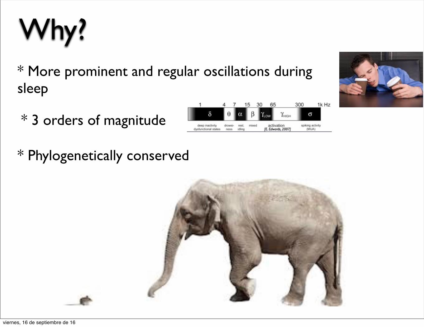
* More prominent and regular oscillations duringsleep
* 3 orders of magnitude
* Phylogenetically conserved
Why?
viernes, 16 de septiembre de 16

* More prominent and regular oscillations duringsleep
* 3 orders of magnitude
* Phylogenetically conserved
Why?
* Change with stimulus, behavior, or disease
viernes, 16 de septiembre de 16
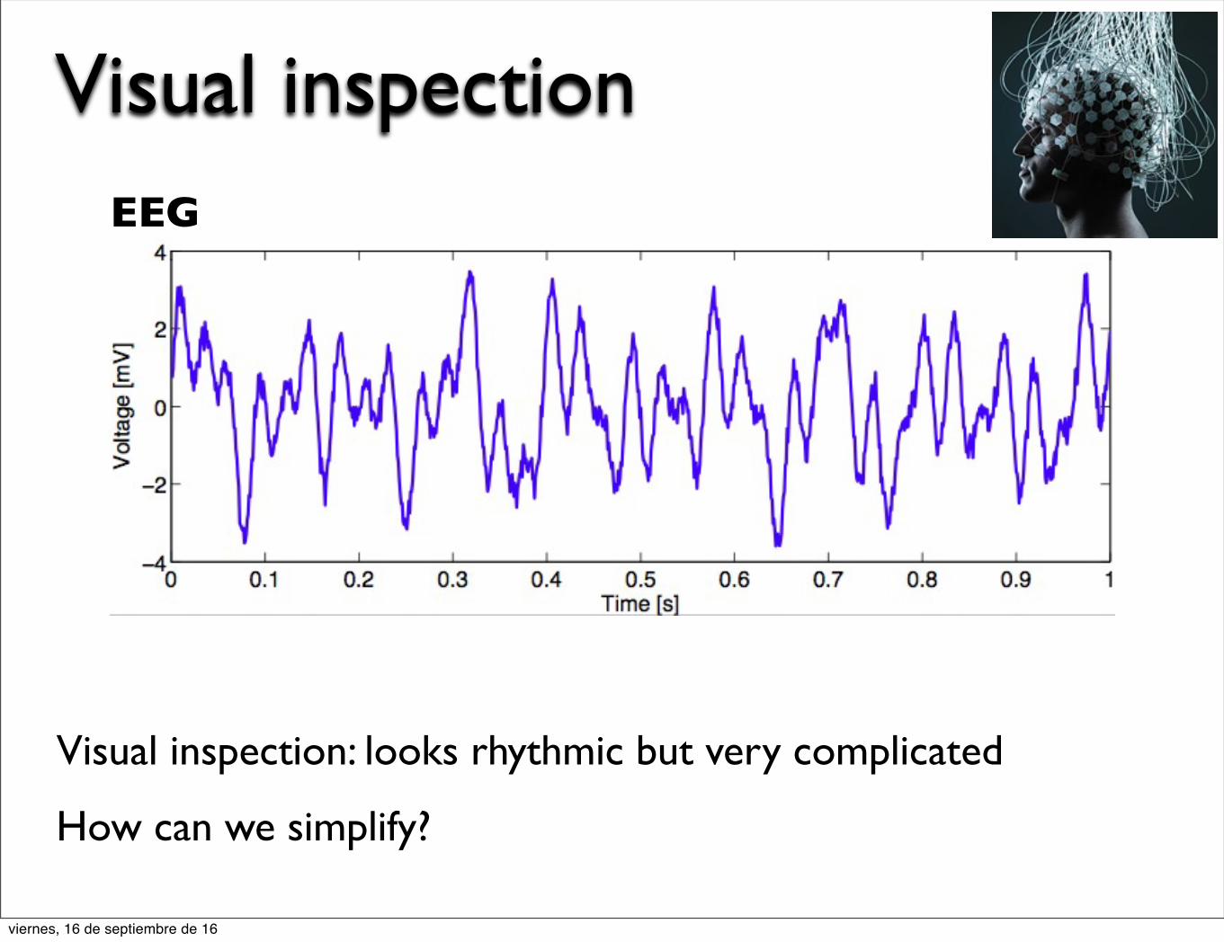
Visual inspectionEEG
Visual inspection: looks rhythmic but very complicated
How can we simplify?
viernes, 16 de septiembre de 16

Visual inspectionEEG
viernes, 16 de septiembre de 16

Power spectrumPower spectrum (EEG)
Axes: Power (dB) vs Frequency (Hz)
Simpler representation in frequency domain. Four peaks at {7, 10, 23, 35} Hz
viernes, 16 de septiembre de 16

Idea
V =
viernes, 16 de septiembre de 16

Idea
V =
Separate the signal into oscillations at different frequencies
+
+
+
+
...
V =
viernes, 16 de septiembre de 16

Idea
V =
Separate the signal into oscillations at different frequencies
A1
A2
A3
A4
f1
f2
f4
f3
+
+
+
+
...
V =
viernes, 16 de septiembre de 16

Idea
V =
Separate the signal into oscillations at different frequencies
A1
A2
A3
A4
f1
f2
f4
f3
+
+
+
+
...
V =
Represent V as a sum of sinusoids (e.g., part 7 Hz, part 10 Hz,...)viernes, 16 de septiembre de 16

Idea
We want to decompose data V(t) into sinusoids
We need to find the coefficients:
Fourier transform
Power (complexcoefficients squared)
Complex coefficients
Sinusoids with better match to V(t) will have larger power
viernes, 16 de septiembre de 16

In practice
fft
>> pow = abs(fft(v)).^2*2/length(v);
To compute the power spectrum in MATLAB use command
Fourier transform
Power (complexcoefficients squared)
viernes, 16 de septiembre de 16
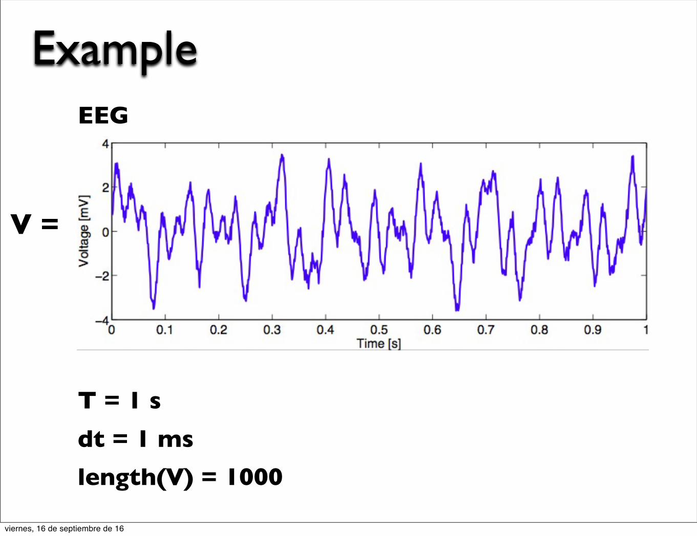
ExampleEEG
T = 1 s
dt = 1 ms
length(V) = 1000
V =
viernes, 16 de septiembre de 16

Example
>> pow = abs(fft(v)).^2*2/length(v);>> pow = 10*log10(pow);>> plot(pow)
MATLAB code 1000 data pts
Matches length of vIncomplete: Must label x-axis?
viernes, 16 de septiembre de 16

Power spectrum x-axisIndices and frequencies are related in a funny way...
Examine vector pow:
Freq
Index
Frequencyresolution
(df)
Nyquistfrequency
(fNQ)
f > 0 f < 0
1000
viernes, 16 de septiembre de 16
Power spectrum x-axis
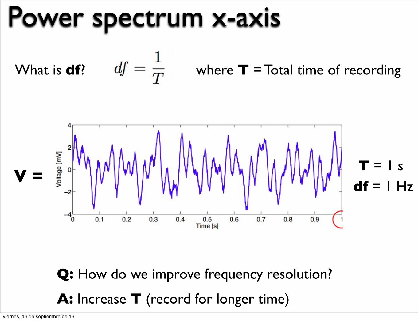
What is df? where T = Total time of recording
V =df = 1 HzT = 1 s
Q: How do we improve frequency resolution?
A: Increase T (record for longer time)viernes, 16 de septiembre de 16
Power spectrum x-axis
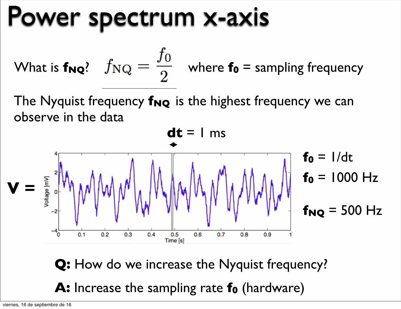
What is fNQ? where f0 = sampling frequency
V =
dt = 1 ms
f0 = 1/dt
Q: How do we increase the Nyquist frequency?
A: Increase the sampling rate f0 (hardware)
The Nyquist frequency fNQ is the highest frequency we can observe in the data
f0 = 1000 Hz
fNQ = 500 Hz
viernes, 16 de septiembre de 16
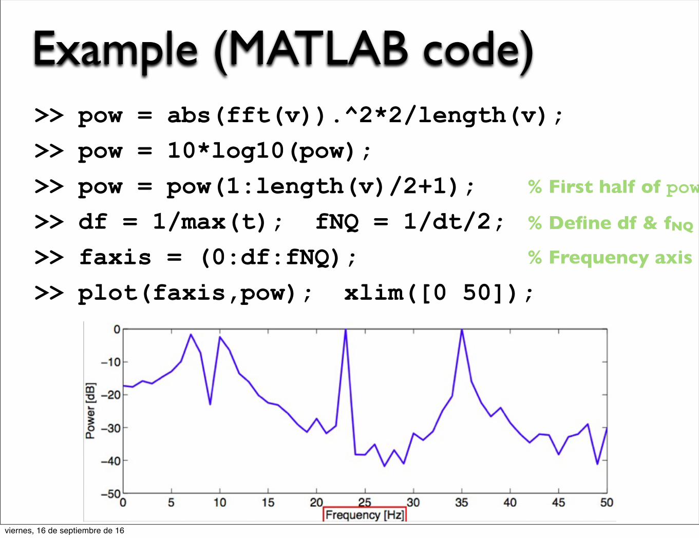
Example (MATLAB code)>> pow = abs(fft(v)).^2*2/length(v);>> pow = 10*log10(pow);>> pow = pow(1:length(v)/2+1);>> df = 1/max(t); fNQ = 1/dt/2;>> faxis = (0:df:fNQ);>> plot(faxis,pow); xlim([0 50]);
% First half of pow
% Define df & fNQ
% Frequency axis
viernes, 16 de septiembre de 16
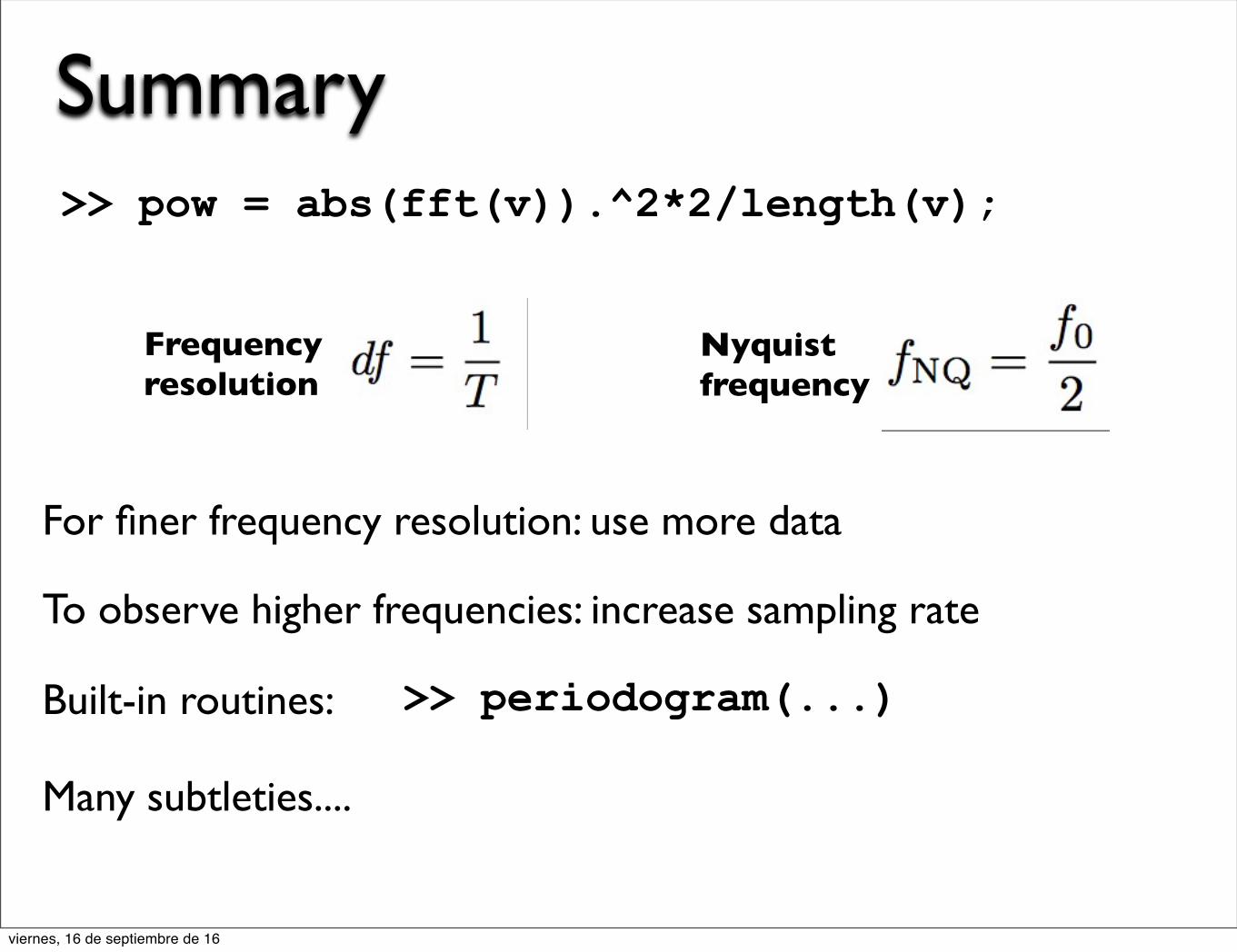
Summary>> pow = abs(fft(v)).^2*2/length(v);
Frequency resolution
Nyquist frequency
For finer frequency resolution: use more data
To observe higher frequencies: increase sampling rate
Built-in routines: >> periodogram(...)
Many subtleties....
viernes, 16 de septiembre de 16

SpectrogramWhat if signal characteristics change in time?
Different spectra at beginning and end of signal
Idea: split up data into windows & compute spectrum in eachviernes, 16 de septiembre de 16

Example (MATLAB code)
>> [S,F,T] = spectrogram(v,1,0.5,1,1000);>> S = abs(S);
>> imagesc(T,F,10*log10(S/max(S(:))));
window
overlap
padding
f0
Plot of power (color) vs frequency and time
A better representation of dataviernes, 16 de septiembre de 16

Network analysis
In many experiments we collect tens or hundreds of channels
An averaged response to a 1kHz toneMagnetic field at 110ms
= auditory M100
How are the activities of different channels related?
viernes, 16 de septiembre de 16

Association measures
Association measures quantify some degree of interdependence between two or more time series:
Correlation (cross-correlation)
Synchronization
Granger causality
Mutual information
...
viernes, 16 de septiembre de 16

Correlation
Y
Y
Y Y
Y Y
X X X
X X
X
X
Given two time series: X = {x1, x2, x3, ... , xn} & Y = {y1, y2, y3, ... , yn}
the correlation coefficient r mesures the linear “similarity” between them
>> r = corr(X,Y);
Y(t) = a*X(t) + w(t) ?
viernes, 16 de septiembre de 16

Cross-correlation
Cross-correlation measure the degree of linear similarity of twosignals as a function of a time shift (lag)
viernes, 16 de septiembre de 16

Cross-correlationThe value and position (lag) of the maximum of the cross-correlation function can give information about the strength and timing of interactions
>> r = xcorr(X,Y,maxlag); % returns a vector r of length 2*maxlag + 1
Y(t) = a*X(t-d) + w(t) ?
viernes, 16 de septiembre de 16

Networks
In structural networks the edges represent physical connections between nodes (synapses or white matter tracts)
Set of nodes and edges
It allows to study a set of channelsas a whole
Functional networks rely on the co-activation or coupling of the dynamics of separate brain areas
viernes, 16 de septiembre de 16

Networks
1 Compute a measure of “coupling” between two channels (e.g. cross-correlation)
2 Draw and edge if the “coupling” > threshold
3 Repeat for all pairs of channels
Network characterize its structure (degree, length, hubs, clusters,...)
viernes, 16 de septiembre de 16

NetworksThe easy way to estimate connectivity: HERMES toolbox
http://hermes.ctb.upm.es
viernes, 16 de septiembre de 16

Default Mode Network (DMN)fMRI (BOLD) Spontaneous modulations
during restingCorrelations (functional
connectivity)
viernes, 16 de septiembre de 16

Continuous signals
Spikes
viernes, 16 de septiembre de 16
Raster plot
Post-stimulus time histogram
Receptive field
Spikes
Spike triggered average
viernes, 16 de septiembre de 16

Spike trains (raster plot)
A spike train is a series of discrete action potentials from a neuron taken as a time series
A raster plot represents spike train along time in the x-axis and cell number (or trial number) in the y-axis
raster plot
viernes, 16 de septiembre de 16

Spike trains (rate)
If properties change over time a more refined measure is the instantaneous rate r(t): r(t)*dt = average number of events between t and t+dt
Each neuron can be characterized by its firing rate r r = average number of events per unit of time
28 spikes/s
64 spikes/s
17 spikes/s
viernes, 16 de septiembre de 16
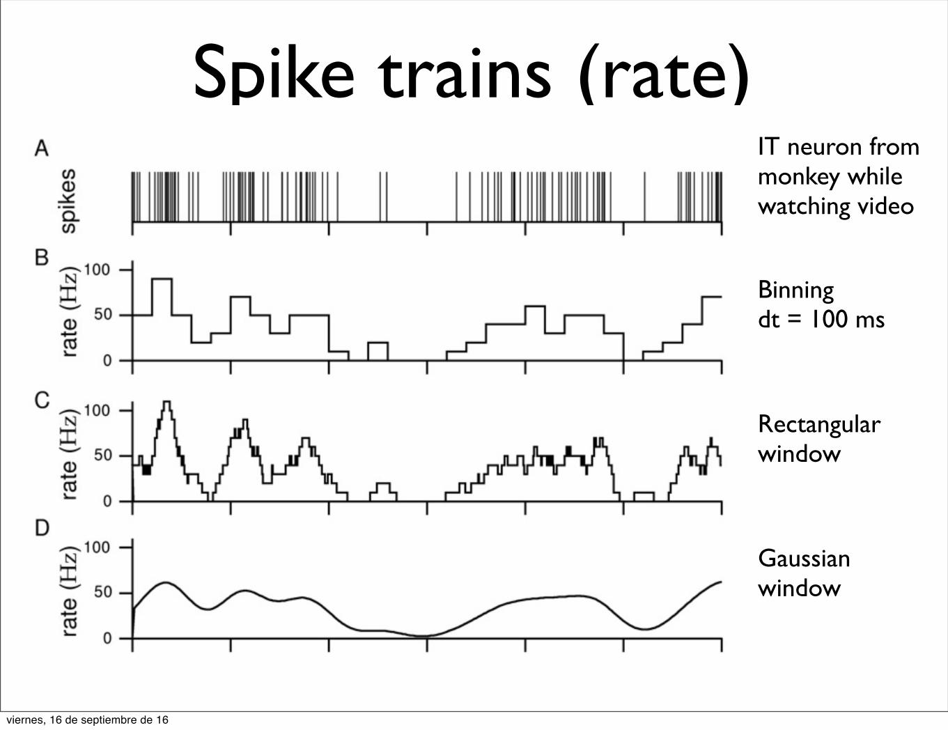
Spike trains (rate)IT neuron frommonkey while watching video
Binning dt = 100 ms
Rectangularwindow
Gaussianwindow
viernes, 16 de septiembre de 16

PSTH is an histogram of the times at which neurons fire
Post-Stimulus Time Histogram
PSTH is used to visualize the rate and timing of spikes in relation to an external stimulus. PSTH/#trials ∼ r(t)
viernes, 16 de septiembre de 16
The receptive field of a neuron is a region of space in which the presence of a stimulus will alter the firing of that neuron
Receptive field
The space can be a region on an animal’s body (somatosensory), a range of frequencies (auditory), a part of the visual field (visual system), or even a fixed location in the space surrounding an animal (place cells)
http://www.youtube.com/watch?v=8VdFf3egwfg
viernes, 16 de septiembre de 16

viernes, 16 de septiembre de 16

The Spike Triggered Average (STA) is the average stimulus preceding a spike
Spike Triggered AverageWhat makes a neuron fire?
viernes, 16 de septiembre de 16

STA from neuron in the electrosensory antennal lobe
Spike Triggered Average (Ex.)Weakly electric fish (Eigenmannia)
viernes, 16 de septiembre de 16
Summary• Event related potentials (ERPs) and post-time
stimulus histograms (PSTH) average the neural responses near some event of interest
• Power spectrum can reveal the presence of rhythms or oscillations in recordings
• Functional networks are defined by the co-activation of separate brain areas
• Receptive fields describes what a neuron is sensitive to
viernes, 16 de septiembre de 16
Applications
Cognitive
Models
Analyses
Basics
Lesson Title
1 Introduction
2 Structure and Function of the NS
3 Windows to the Brain
4 Data analysis
5 Data analysis II
6 Single neuron models
7 Network models
8 Artificial neural networks
9 Learning and memory
10 Perception
11 Attention & decision making
12 Brain-Computer interface
13 Neuroscience and society
14 Future and outlook: AI
15 Projects presentations
16 Projects presentations
viernes, 16 de septiembre de 16
Recommended