
Lecture 4
• Recall that we are interested in learning about
models
• In this chapter, we will learn about
– behavior of the representative consumer
– behavior of the representative firm
4-1
4-2
Representative Consumer
• Consumer’s preferences over consumption and leisure as represented by indifference curves.
• Consumer’s budget constraint.
• Consumer’s optimization problem: making his or herself as well off as possible given his or her budget constraint.
• How does the consumer respond to: (i) an increase in non-wage income; (ii) an increase in the market real wage rate?

Let’s first look at the consumer preferences
4-4
Representative Consumer’s
Indifference Curves
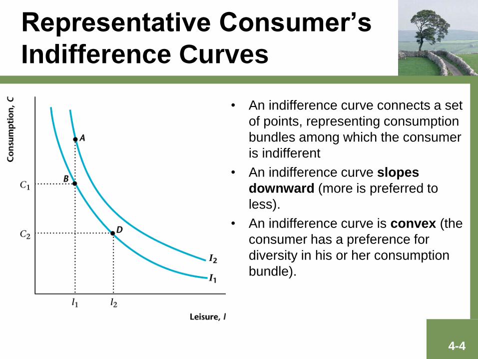
• An indifference curve connects a set
of points, representing consumption
bundles among which the consumer
is indifferent
• An indifference curve slopes
downward (more is preferred to
less).
• An indifference curve is convex (the
consumer has a preference for
diversity in his or her consumption
bundle).
4-5
Properties of Indifference
Curves
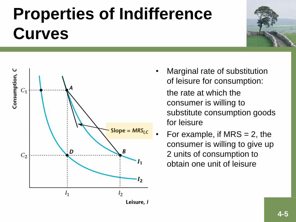
• Marginal rate of substitution
of leisure for consumption:
the rate at which the
consumer is willing to
substitute consumption goods
for leisure
• For example, if MRS = 2, the
consumer is willing to give up
2 units of consumption to
obtain one unit of leisure

Now let’s look at the constraints that the consumer
faces
4-7
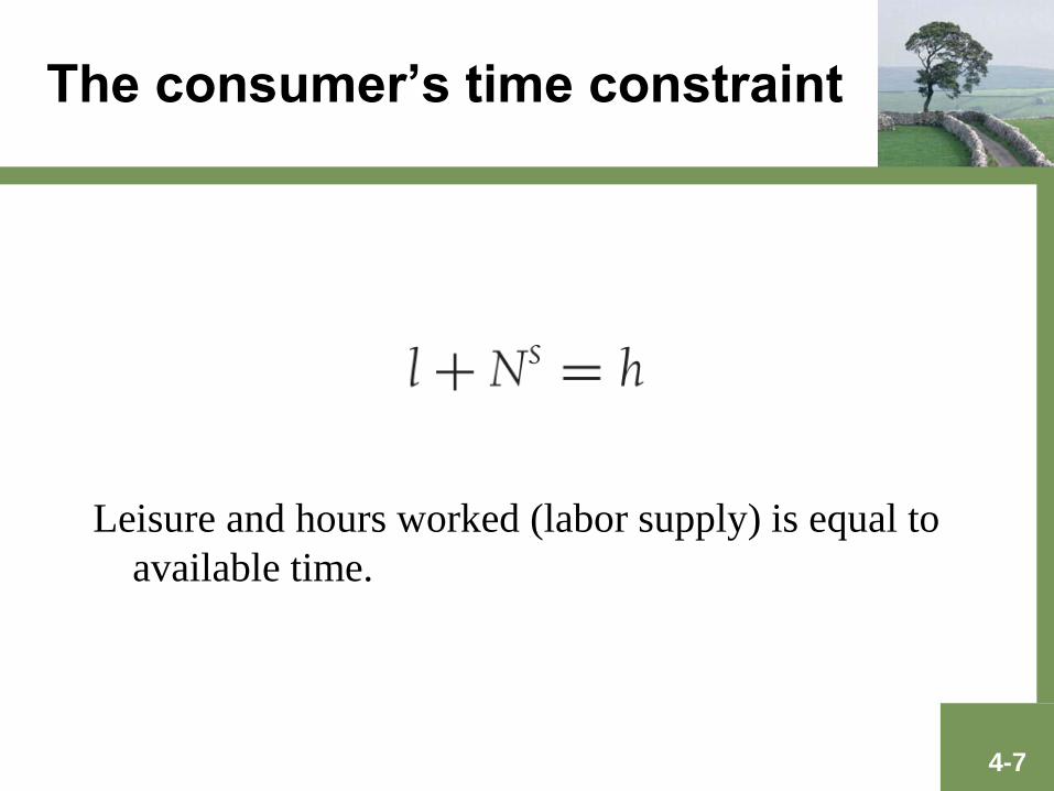
The consumer’s time constraint
Leisure and hours worked (labor supply) is equal to
available time.
4-8
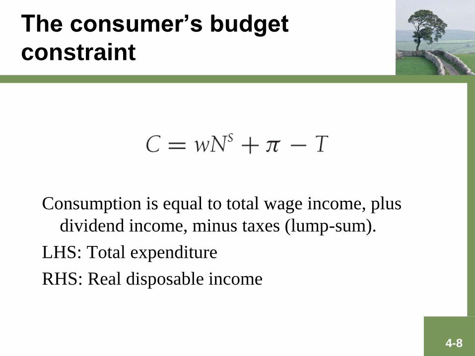
The consumer’s budget
constraint
Consumption is equal to total wage income, plus
dividend income, minus taxes (lump-sum).
LHS: Total expenditure
RHS: Real disposable income
4-9
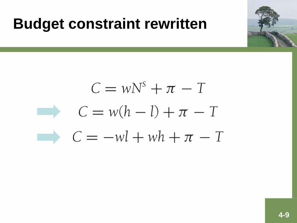
Budget constraint rewritten
4-10
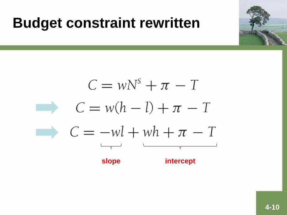
Budget constraint rewritten
slope intercept
4-11
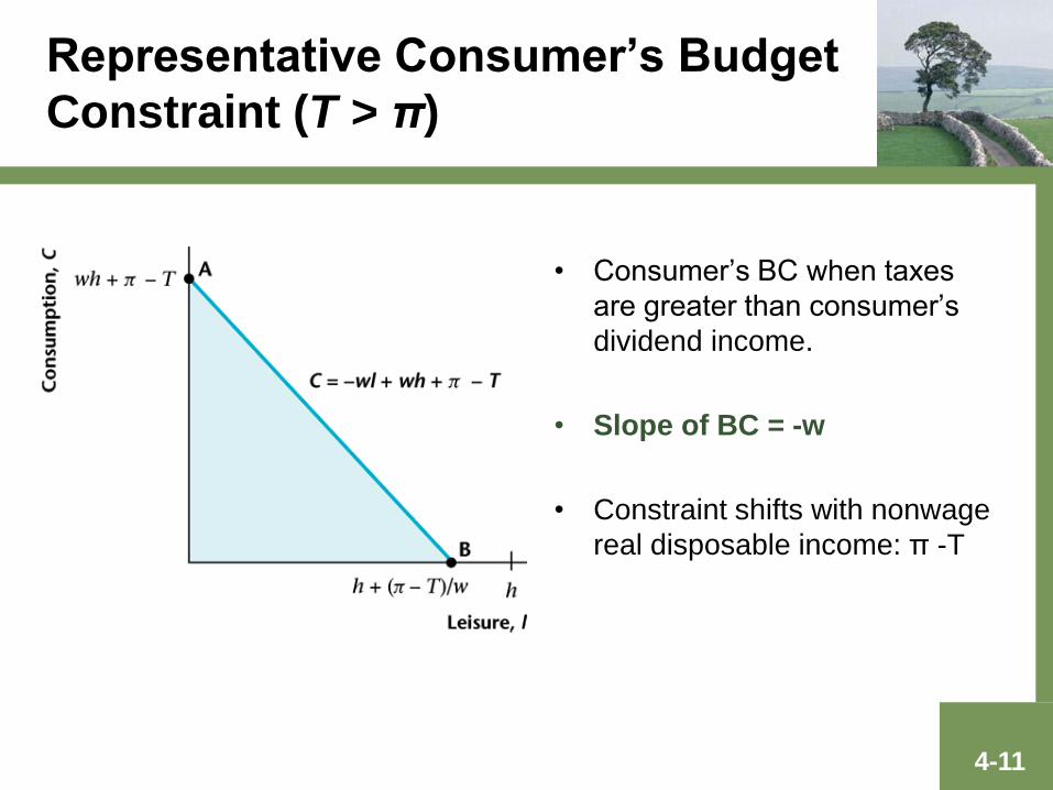
Representative Consumer’s Budget
Constraint (T > π)
• Consumer’s BC when taxes
are greater than consumer’s
dividend income.
• Slope of BC = -w
• Constraint shifts with nonwage
real disposable income: π -T
4-12
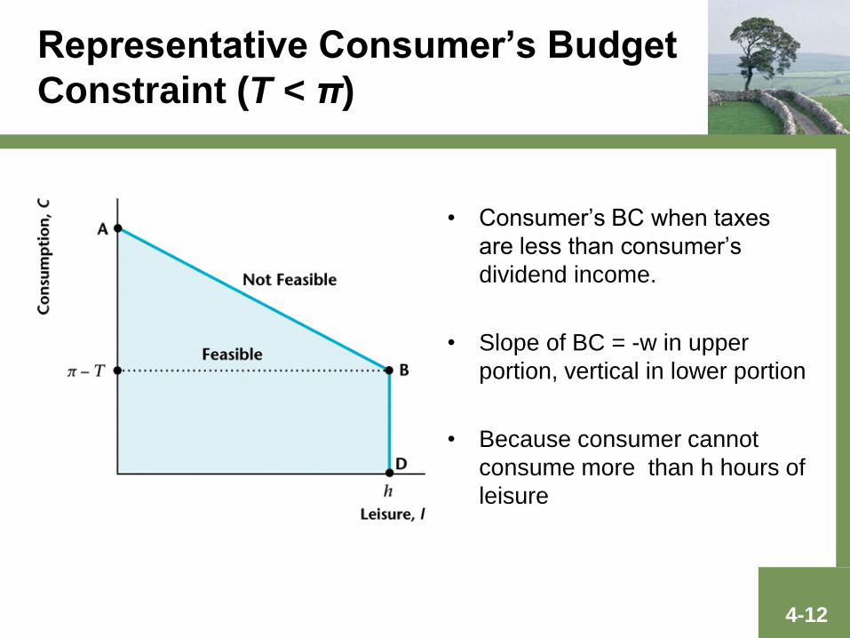
Representative Consumer’s Budget
Constraint (T < π)
• Consumer’s BC when taxes
are less than consumer’s
dividend income.
• Slope of BC = -w in upper
portion, vertical in lower portion
• Because consumer cannot
consume more than h hours of
leisure
4-13
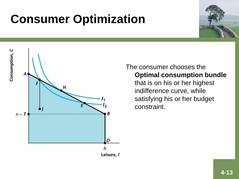
Consumer Optimization
The consumer chooses the
Optimal consumption bundle
that is on his or her highest
indifference curve, while
satisfying his or her budget
constraint.

4-14
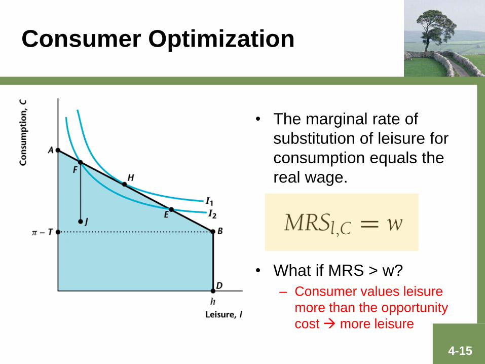
Consumer Optimization
• The marginal rate of
substitution of leisure for
consumption equals the
real wage.
• What if MRS > w?
4-15
Consumer Optimization
• The marginal rate of
substitution of leisure for
consumption equals the
real wage.
• What if MRS > w?
– Consumer values leisure
more than the opportunity
cost more leisure
4-16
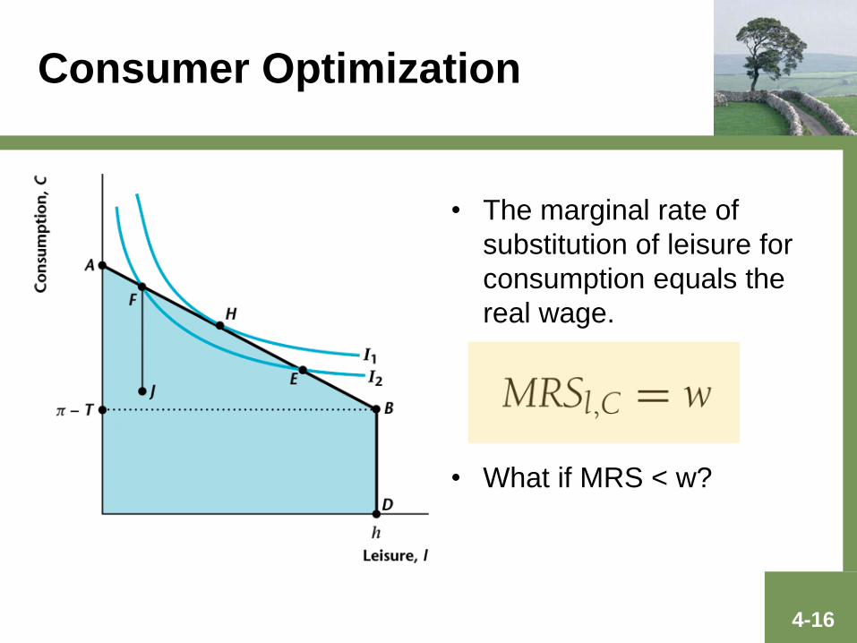
Consumer Optimization
• The marginal rate of
substitution of leisure for
consumption equals the
real wage.
• What if MRS < w?

4-17
Consumer Optimization
• The marginal rate of
substitution of leisure for
consumption equals the
real wage.
• What if MRS < w?
– Consumer values leisure
less than the opportunity
cost less leisure
4-18
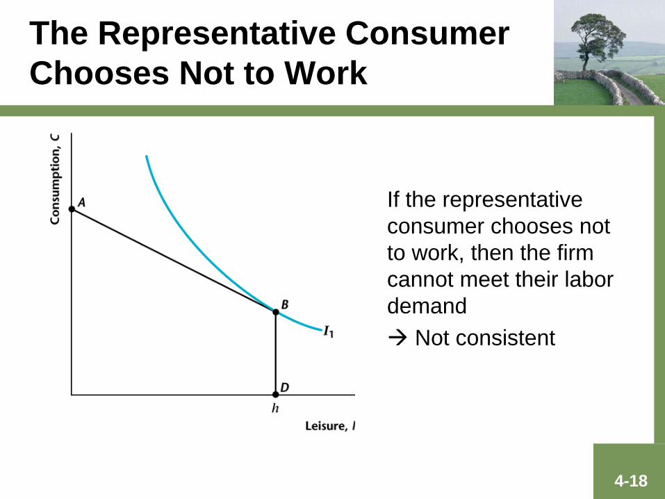
The Representative Consumer
Chooses Not to Work
If the representative
consumer chooses not
to work, then the firm
cannot meet their labor
demand
Not consistent
Comparative Statics
• What if real dividends increase or taxes
decrease?
• What if real wages increase?
4-19
4-20
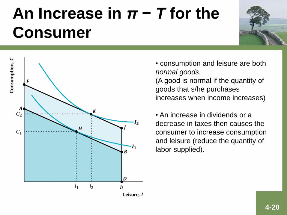
An Increase in π − T for the
Consumer
• consumption and leisure are both
normal goods.
(A good is normal if the quantity of
goods that s/he purchases
increases when income increases)
• An increase in dividends or a
decrease in taxes then causes the
consumer to increase consumption
and leisure (reduce the quantity of
labor supplied).
4-21
An increase in the market real
wage rate
• This has income and substitution effects.
• Substitution effect: the price of leisure rises, so the
consumer substitutes from leisure to consumption.
• Income effect: the consumer is effectively more
wealthy and, since both goods are normal, consumption
increases and leisure increases.
• Conclusion: Consumption must rise, but leisure may
rise or fall.
4-22
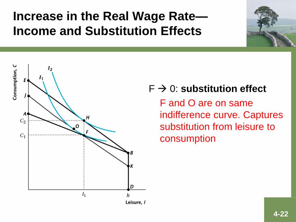
Increase in the Real Wage Rate—
Income and Substitution Effects
F 0: substitution effect
F and O are on same
indifference curve. Captures
substitution from leisure to
consumption

4-23
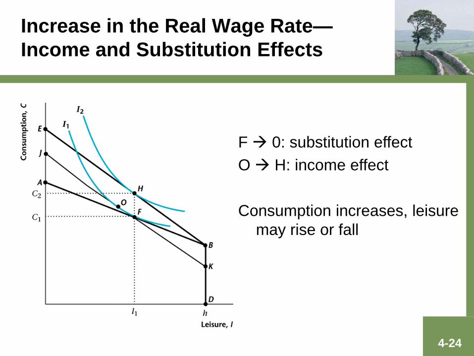
Increase in the Real Wage Rate—
Income and Substitution Effects
O H: income effect
EB and JK have the same
slope. Captures increase in
consumption and leisure in
response to pure income
effect
4-24
Increase in the Real Wage Rate—
Income and Substitution Effects
F 0: substitution effect
O H: income effect
Consumption increases, leisure
may rise or fall
4-25
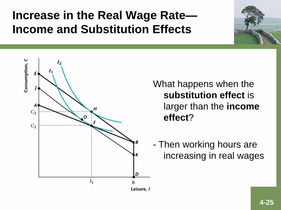
Increase in the Real Wage Rate—
Income and Substitution Effects
What happens when the
substitution effect is
larger than the income
effect?
- Then working hours are
increasing in real wages
4-26
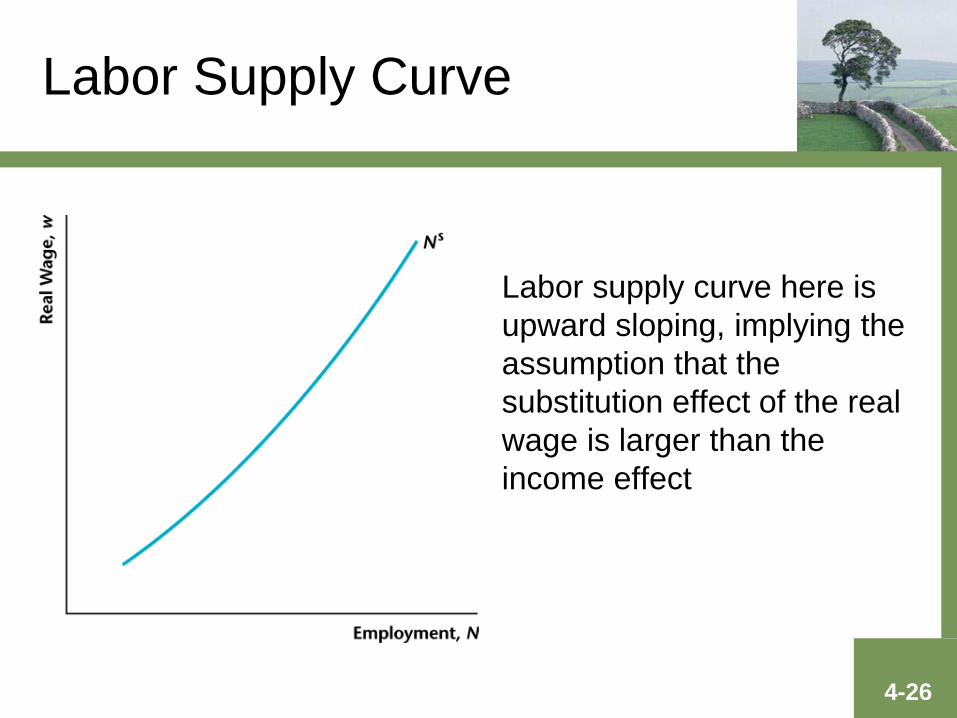
Labor Supply Curve
Labor supply curve here is
upward sloping, implying the
assumption that the
substitution effect of the real
wage is larger than the
income effect
4-27
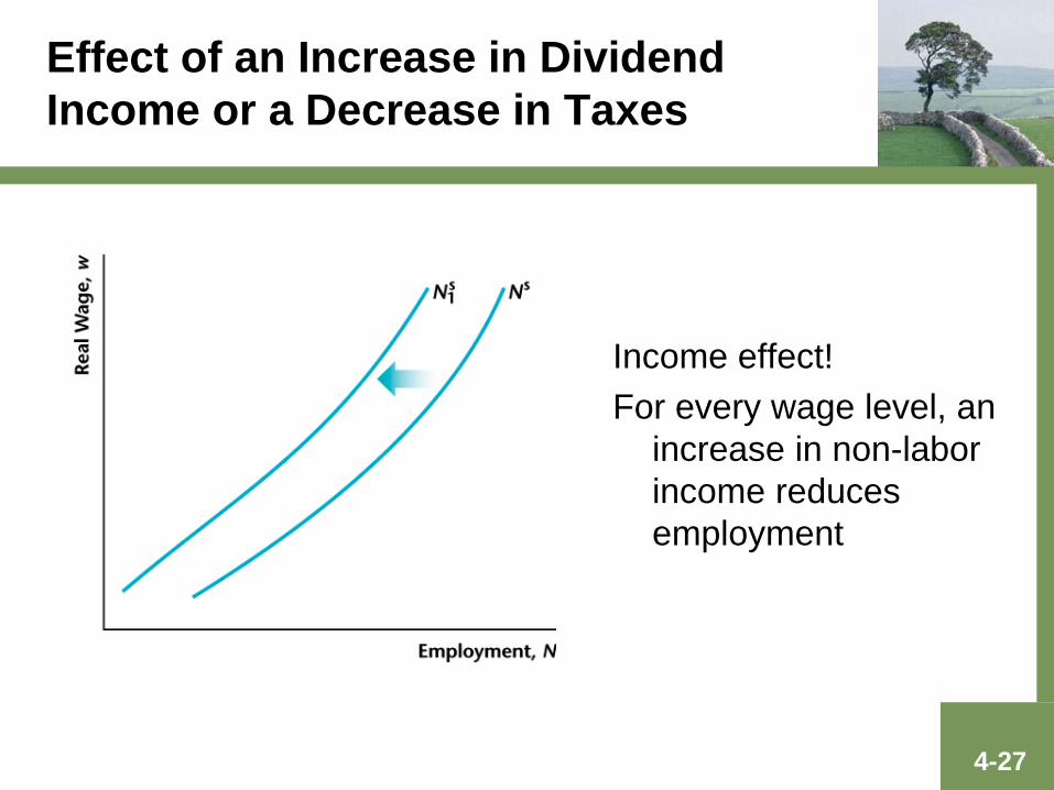
Effect of an Increase in Dividend
Income or a Decrease in Taxes
Income effect!
For every wage level, an
increase in non-labor
income reduces
employment

4-28
Any questions?
We are now ready to look at handout 1!
Recommended