
ISSN 1836-8123
Series Editor: Dr. Alexandr Akimov
Copyright © 2012 by author(s). No part of this paper may be reproduced in any form, or stored in a retrieval system, without prior permission of the author(s).
Marginal abatement cost curves and carbon capture and storage options in Australia
Jason West
No. 2012-02
1
Marginal abatement cost curves and carbon capture and storage options in Australia
Jason West1
Abstract
Griffith University
Marginal abatement cost curves are a principal tool used for measuring the relative economic
impact of emissions abatement mechanisms. Abatement curves can be constructed using
either a top-down approach based on aggregated microeconomic models or using a bottom-
up approach based on an engineering assessment that analyses different technical potentials
for emission reductions. While top-down models offer simplicity and ease of interpretation,
they are not as robust as the bottom-up approach, particularly for assessing the implications
of new technologies such as carbon capture and storage (CCS). Using a bottom-up approach
and incorporating real options analysis, this study redefines the relative abatement costs for
retrofitting post-combustion CCS technology to coal-fired generators and then reconstructs
the Australian marginal emissions abatement curve. The revised curve provides power
generators and other industry sectors with more accurate and stable abatement cost estimates
for these technologies relative to alternate abatement options.
Key words: Carbon sequestration, coal, energy production, emissions abatement, real
options.
JEL: Q54, Q58, Q41, G13
1
Department of Accounting, Finance and Economics, Griffith Business School, Nathan, QLD, Australia, 4111, +61 7
37354272 (w), email: [email protected]
2
1. Introduction Marginal abatement cost curves (MACCs) are one of the principal tools used to measure the
relative economic impact of emission abatement mechanisms. A MACC can be derived for a
firm, an industry sector or a geographic region. The core advantage of an abatement curve is
that it can provide a reasonably simple interpretation of the relative and total abatement costs
for various abatement activities and technologies aimed at reducing greenhouse gas
emissions. An abatement curve can be constructed not only for carbon-dioxide (CO2) but for
any pollutant (McKitrick, 1999). MACCs for reducing greenhouse gas (GHG) emissions
have become an important tool for estimating the major economic impacts of national GHG
reductions policies (Johnson, 2002; Klepper and Peterson, 2006) and have also been used in
an environmental economic context to identify efficient and practical policy solutions aimed
at reducing the net social cost of climate change policies (Lee, 2005).
MACCs can be constructed in two major ways. Firstly a top-down approach based on
aggregated microeconomic models and cost functions and/or related distance functions can
be used. Secondly a bottom-up model based on an engineering assessment that analyses
different technical potentials for emission reductions can be employed. The MACC derived
using a top-down approach to aggregate economic models is often used to develop broad
climate change policy settings and to assess investment opportunities in both government and
industry settings. While abatement curves derived using this method are relatively simple to
use in an economy-wide context, they are not as accurate or robust as the bottom-up approach
for assessing the implications of new technologies. Due to the aggregation of abatement
activities, top-down models generally ignore a range of specific technical capabilities that can
be employed at the plant level. When aggregated, the plant level activities can offer
significant abatement advantages than aren’t identified during the top-down approach.
Misapplication of emissions abatement opportunities at the firm or industry sector level can
damage the long term competitiveness of a firm or industry which results in sub-optimal
abatement decisions.
The top-down approach for constructing MACCs also ignores the economic impact of
recursive feedback from explicit emissions prices imposed on industry sectors. For instance,
in the presence of an emissions tax or permit scheme the additional costs to power generators
from increased fuel costs due to fugitive emissions incurred from coal mining and gas

3
extraction is either ignored or a simple baseline cost is applied to all emitters. At the plant or
mine level however, the actual consumption of fuel containing fugitive emissions penalties as
well as local abatement opportunities using small-scale technical solutions can significantly
alter the abatement cost. The top-down approach also ignores the flexibility in the timing of
building technology options when it is optimal to do so.
A MACC has been constructed for Australia using the top-down approach (McKinsey, 2008).
The Australian MACC is widely used for emissions policy analysis and for prioritising
abatement technology funding by both industry and government. This analysis reconstructs
the Australian MACC using a bottom-up approach to assess a specific and significant
abatement option available to power generators – post-combustion carbon capture and
storage (CCS). This analysis includes the feedback costs of higher input fuel prices
associated with fugitive emissions and the value of managerial optionality and economic
incentives. The result of using this approach redefines the relative abatement costs associated
with retrofitting CCS technology to existing coal-fired power plants. The revised abatement
curve demonstrates the true economics of CCS technology by aggregating plant-level costs
and our analysis reveals the optimal timing for retrofitting CCS to each plant in Australia
using real option valuation. It is shown that imposing an explicit price on emissions should
alter the research and development incentives for CCS technology and lead to the
development of commercial scale plants at a cost advantage ahead of alternate energy
sources.
Section 2 describes the alternative approaches for constructing the MACC in the Australian
context. Section 3 introduces the model framework. Section 4 presents and discusses the
results. Section 5 offers some concluding remarks.
2. Construction of the Australian marginal abatement curve 2.1. Australia’s energy mix
The composition of electricity supply in Australia in the period 2011 to 2030 will be
influenced by a number of factors, most notably:

4
• government policy settings for renewable energy, in particular mandatory renewable
energy targets;
• the cost and availability of different fuel sources (the costs of fuel will partly depend
on the price signal for CO2);
• the cost of competing generation technologies;
• the extent to which alternative technologies are commercialised;
• societal attitudes towards alternative generation and abatement technologies; and
• the capacity of transmission and interconnection infrastructure as well as the
regulatory framework.
Australia’s energy mix is dominated by fossil fuels. Figure 1 provides a history and IEA
forecast of installed generation capacity by plant type for 1998-2030. Coal and gas made up
around 77 percent of installed capacity and almost 89 percent of annual production in 2010.
Figure 1 illustrates a significant decline in capacity from 2018 which coincides with the
expected phased decommissioning of several coal and gas generation units. Since Australia’s
power demand is not expected to decline in line with this projection but increase over this
period, the gap in generation capacity encourages analysis of what energy alternatives will be
cost effective after this point. A gap of at least 10GW of generating capacity by 2020
represents a significant investment opportunity for energy generators however the source of
this power will depend on the expected investment returns of the range of alternatives
available.

5
Figure 1: Installed electricity generation capacity (GW) in Australia 1998-2010 and forecast 2011-2030 by
fuel type. Forecast obtained from IEA (2009) projections.
In 2010 the Australia’s installed energy capacity was approximately 47 GW which produced
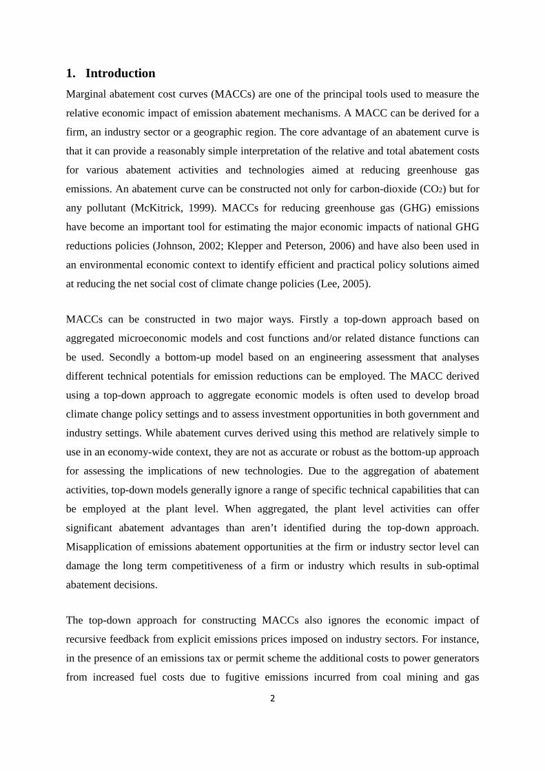
around 207 TWh of electricity. Australia’s energy intensity, calculated as units of energy per
unit of GDP, has historically been in line with most western countries and is projected to
continue at this rate to 2030. This is illustrated in Figure 2 alongside the levels of energy
intensity projected for France, Germany and the US as a comparison. Energy demand is
expected to continue to grow at a rate consistent with GDP growth, moderated by the
efficiencies implied by improved energy intensity.
Ex
6
Figure 2: The energy intensity of Australian electricity industry relative to the energy intensity levels of
the US, France and Germany (1998 base year), IEA (2009).
The choice of power generation unit depends inter alia on liabilities associated with the cost
of construction, operating and maintenance costs and input fuel prices which then dictates the
unit’s merit order for power dispatch. The choice of generation unit due to the expected
growth in power demand and the forecast shortfall in capacity in Australia will need to
include an explicit price on emissions. Such an imposition of a price on emissions may
greatly alter Australia’s energy mix due to an expected shift in the merit order away from
fossil fuels to other alternatives, particularly for baseload electricity generation.
2.2. The Australian CO2 abatement cost curve
In the context of energy source selection the challenge lies in finding affordable means for
reducing greenhouse gas emissions. Marginal emissions abatement curves are used to
illustrate the economic benefits and likelihood of climate change mitigation projects. The
notion of a marginal abatement cost curve (MACC) is derived from firm or plant level
models for reducing greenhouse gas and other emissions, but is generally applied at an
aggregate level. From contemporary production theory the interpretation of the MACC is
straightforward. Given that certain activities in the production process lead to emissions of
undesired pollutants and assuming the availability of certain abatement technologies, the
marginal abatement cost represents either the marginal loss in profits from avoiding the last
unit of emissions or the marginal cost of achieving a certain emission target given some level
of output. While the latter focuses on abatement technologies to prevent the release of
7
pollutants, the former focuses on the economic reaction of a firm to an emission constraint
(McKitrick, 1999). This includes adjustments by the firm to the level of output. The concept
of a MACC was adopted for climate policy analyses in the context of a general equilibrium
framework and has been championed by McKinsey & Company in assessing abatement
options by industrial sector and geographic region (McKinsey, 2007).
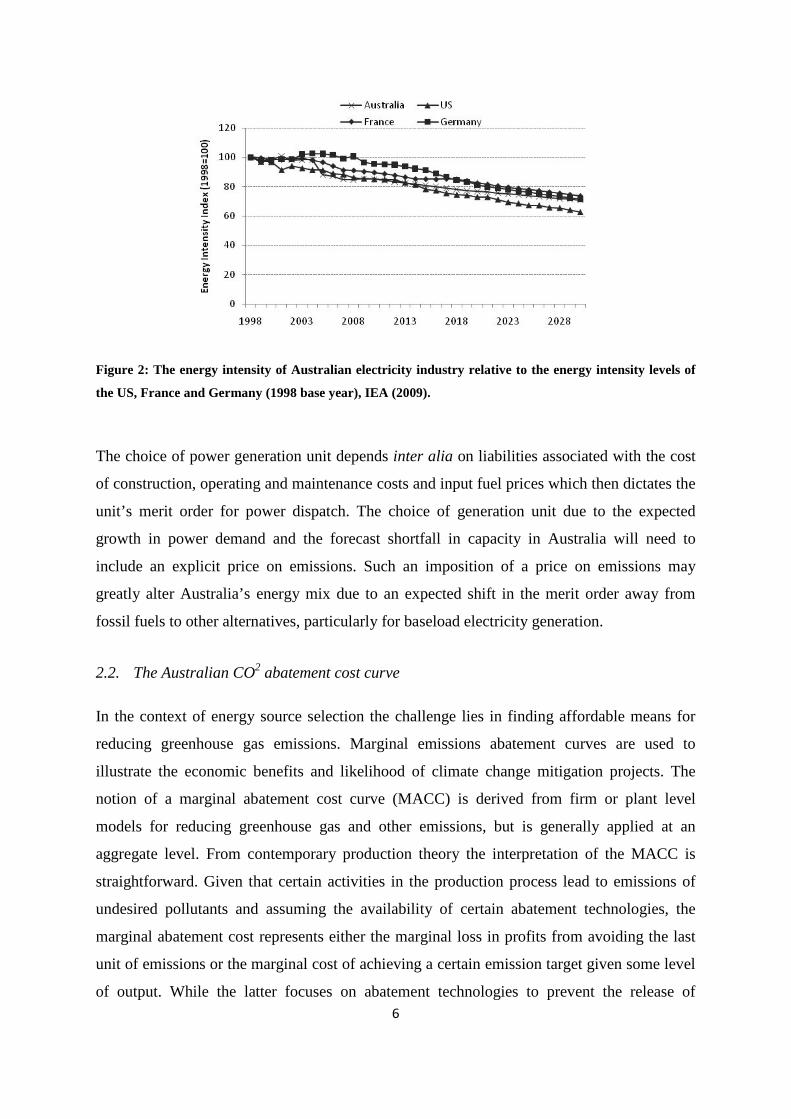
Figure 3 is a reproduction of the abatement curve for Australia (McKinsey, 2008) with the
CCS retrofit opportunities highlighted. The curve presents an estimate of the maximum
potential of all technical GHG abatement measures below A$50/tCO2 if each abatement
option were pursued and successfully implemented. The cost curve illustrates abatement
potential and corresponding cost for abatement options relative to a reference case. For this
study the reference case is business-as-usual (BAU) for Australia with minimal abatement
incentives and no explicit price on CO2.
Figure 3: Australian 2030 CO2 abatement cost curve. Abatement opportunities are not accumulated with
those of previous years. Source: McKinsey Australia Climate Change Initiative, 2008.
Abatement potential is defined as the volume difference between an emissions baseline
scenario (BAU) and the level of emissions after an abatement mechanism has been applied.
60
80
100
120
-20
-40
-60
40
200 300 400 500 6001000
20
-80
-100
-120
-140
-160
-180
Abatement cost, A$ per tCO2e
Motor systems
Commercial air handling
Geothermal
Solar PV
Coal CCS retrofit
Abatement potentialMtCO2e per year
Af forestation, pasture
Forest management
Onshore wind
Coal CCS newIndustrial CCS
Avoided deforestation
Biomass
Afforestation, cropland
Coal to gas shif ts, new-builds
Agriculture (soils and livestock)
Conservation tillage
Car fuel economy
Residential heating ef f iciencies
8
The width of each column represents the economic potential of an abatement mechanism that
results in a reduction of emissions using the abatement option over the scenario period. Note
that the column widths represent potential abatement volumes and are not an actual forecast
of abatement activities. The height of each column is the average cost of avoiding a tonne of
CO2 from each abatement opportunity. Abatement costs are the incremental cost of a low-
emissions mechanism compared to the reference case measured as a dollar per tonne of CO2
avoided. Abatement costs include annualised capital and operating expenditure which
attempts to replicate the project cost of installing and operating the technology (McKinsey,
2007). The abatement cost AC is computed as
, (1)
where is the full cost of the CO2 efficient alternative, is the full cost of the
reference case, is the volume of CO2 emissions from the CO2 efficient alternative and
is the volume of CO2 emissions from the reference solution over the scenario period
(2010-30).
As shown in Figure 3 the economy-wide MACC for Australia identifies the cost of reducing
an additional unit of CO2 from the BAU emissions level. Each additional unit of emission
reduction generally has incrementally higher cost leading to the formation of a convex curve
with increasingly positive slope. Similarly a firm-specific MACC links a firm’s emission
levels to the cost of reducing one unit of emissions from the current level and is a key tool for
optimising firm-related abatement opportunities (McKitrick, 1999). At the system level
MACCs can be used to determine which sector(s) to focus on to abate emissions in the most
cost-effective manner.
In this study we focus on the impact on the Australian MACC of retrofitting existing coal-
fired generation assets with post-combustion CCS technology accounting for the influence of
fugitive emissions on fuel input costs and managerial flexibility in the timing of the capital
investment.
2.3. Abatement curve modelling alternatives
9
Two general types of models are used to analyse abatement alternatives and generate the
MACC for a given region or industry. The first is a top-down model based on an aggregated
microeconomic model and cost function approach (Gollop and Roberts, 1985) or distance
function approach (Fare, et.al., 1993; Lee, Park and Kim, 2002). When using either approach
the marginal abatement cost is calculated as the shadow price of reducing emissions by one
unit or alternatively the opportunity cost of reducing the level of output by one unit. In this
context the marginal abatement cost is defined as the shadow cost produced by a constraint
on CO2 emissions for a given region and period. The shadow cost is equivalent to the tax that
would have to be levied on the emissions to achieve the targeted level or the price of an
emission permit in the case of an emissions trading scheme. This is the general approach
taken by McKinsey (2008) for the construction of the MACC for Australia.
While the cost function and output distance function methods can roughly indicate the cost of
reducing emissions by way of reducing the output, these approaches do not explicitly
consider any end-of-pipe (EOP) or change-in-process (CIP) control technologies to reduce
emissions. For example, Coggins and Swinton (1996) clearly showed their inability to
incorporate important technology options such as scrubbers to arrive at estimates of the cost
of sulphur-dioxide allowances from coal-fired generators. Because these approaches only
consider changes in output, a specific EOP or CIP control may have a lower marginal
abatement cost than the shadow price estimated using the top-down approach. Further, the
actual opportunity cost of forgoing production may be higher than estimated in a case where
plant efficiency decreases with a reduction in the output. Firms also generally fail to
minimise their production cost in the presence of various regulations and so the cost-function
approach is likely to underestimate the marginal abatement cost (Lee, 2005).
Bottom-up models are based on a plant-by-plant engineering-economic approach that
measures different technical potentials for emission reductions by power generator or CO2
emitter (Beaumont and Tinch, 2004; Karvosenoja and Johansson, 2003) and then aggregates
abatement potential for the system. Different levels of a shadow carbon tax are levied on
coal-fired power generators depending on plant specific factors such as thermal efficiency,
proximity to fuel sources and capacity for retrofitting CCS. This will lead to adjustments in
the final energy demand and to the corresponding levels of emission reductions via
technological or implicit behavioural changes, as well as the replacement of energy
10
conversion systems for which the technologies are explicitly defined. This approach is made
difficult by the requirement for in-depth, plant-specific technical information, firm-specific
proprietary control technology and cost information, and a sound technical understanding of
the construction and operation of the control technologies. Successful working examples of
bottom-up engineering-economic models include the Regional Air Pollution Information and
Simulation (RAINS) model used for predicting acid rain in the European Union and Asia and
MARKAL developed by the Energy Technology Systems Analysis Programme (ETSAP) of
the International Energy Agency.
While top-down methods provide useful information for general analysis and policy making,
the information is rarely useful to managers or decision-makers at the generator level, as it
does not capture plant and technology-specific details related to changes in fuel prices and
the integration of CCS. Likewise cost engineering tools for individual generators capture the
technology and process details for various abatement options, but cannot be readily used to
assess sector-wide costs and tradeoffs among plants. This analysis bridges this
methodological gap by demonstrating a new bottom-up method to create an aggregated
MACC based on individual generator data for Australia. The revised MACC can then be used
to determine how the retrofit costs and emissions reductions associated with individual plants
compare with the entire system.
3. Bottom-up model of marginal abatement The variation of marginal abatement costs across sources of GHGs is highlighted by sectoral
modelling of abatement actions (Weyant, 1999). Reducing coal combustion for instance,
which has the highest CO2 emissions per unit of energy is often among the least costly
abatement option. But for Australia’s baseload energy needs coal-fired generation is likely to
dominate the energy mix given the low cost of domestic coal. A pervasive and uniform
emission price signal applied across the energy sector will encourage abatement actions such
as retrofitting CCS.
3.1. Carbon capture and storage
Carbon capture and storage (CCS) is a technique that prevents CO2 generated from large
stationary sources such as coal-fired power generators from entering the atmosphere. The
technology seeks to capture around 90 percent of CO2 emissions from these generators and

11
permanently prevent their release into the atmosphere by capturing and compressing the CO2
and then transporting it to a storage location. Storage of the CO2 is likely to be in deep
geological formations, in deep ocean masses or stored in the form of mineral carbonates.
The three principal capture processes that are vying for commercial acceptance in the next 20
years are oxy-fuel combustion, post-combustion capture and pre-combustion. Oxy-fuel and
pre-combustion technologies look to increase the concentration of CO2 in the flue gases with
the full exhaust stream being captured. In contrast the simpler post-combustion capture
technology removes CO2 from exhaust gases through absorption by certain solvents. This
analysis will focus on post-combustion capture since the technology is more advanced than
pre-combustion alternatives and sufficient cost data is available.
Post-combustion capture technology is an EOP control technology capable of high
performance and is likely to be a primary technique used for new power plants and
retrofitting existing power plants in Australia from 2011 to 2030. At current estimates the
type of CCS technology employed will not significantly affect the total cost of capture for a
large scale plant, even though the shares of capital and operating expenditure as well as fuel
prices vary significantly across technologies.
The post-combustion capture system generally consists of three parts; the direct contact
cooler, the absorber and the regenerator. Flue gas is exposed to cool water in the contact
cooler which cools and saturates the flue gas post-combustion. This cooler also performs the
desulphurisation process. A chemical reagent solution is combined with the cooled and
saturated flue gas in the absorber. The reagent reacts with the CO2 to form a stable compound
that remains in solution. The CO2-rich solution is then fed to the regenerator where it is
heated and stripped with steam to remove the CO2, which is then transported and sequestered.
Capturing CO2 accounts for about three-fourths of the total cost of a capture, storage,
transport and sequestration system (Rubin, Rao and Berkenpas, 2001; Riahi et.al, 2004),
assuming that CO2 is captured from flue gases by currently available chemical absorption
systems.
The post-combustion analysis accounts for added fuel consumption, parasitic power demand,
reduced plant efficiency and the associated costs of CO2 sequestration. The cost varies by

12
plant type and capacity. Costs also vary depending on the volume of CO2 to be sequestered
and the availability of a suitable site may be limited.
The constant annual output Q in MWh of a power plant using technology n is
, (2)
where is the installed capacity of the generator in MW, c is the capacity factor, is
auxiliary power consumption as a proportion of the total and 8766 represents the number of
hours per annum. The capacity factor incorporates plant availability at baseload and peak
times and the average duration for which the generator is ahead of the marginal supplier in
the merit order. Average plant availability for coal-fired generators varies from 82 percent to
88 percent. The annual output figure is the quantity of electricity generated and dispatched to
the market via the Australian Energy Market Operator (AEMO).
Upon introduction of an explicit emissions price incremental fuel cost increases will be
dependent on the level of the emissions price and the magnitude of fugitive emissions during
the extraction process. The fuel cost in A$/MWh for technology n is a function of the fuel
prices f, the cost pass through associated with fugitive emissions , the rate of net fuel
efficiency (already accounting for auxiliary power consumption) and 3.6 is a general
conversion factor for energy (watt hours to joules) defined as
. (3)
The annual cost of CO2 transport and storage in A$/MWh is represented by the product
of the capture rate r, the annual emissions e and the total capital and operating cost of
transport and storage divided by the output of the capture plant
, (4)
where the annual emissions e in tonnes of CO2 are calculated as
13
, (5)
where is the CO2 emission factor in kt/PJ of fuel consumed. The numerator calculates the
volume of emissions and the denominator adjusts this for the fuel efficiency of the
technology. Note that the cost of CO2 capture is a component of the operating and
maintenance cost for the capture technology.
Net revenue from electricity output for technology n is calculated as
, (6)
where is the constant annual output in MWh, is the average dispatch price, is the
average operating and maintenance cost, is the fuel cost including fugitive emission costs
that are passed through, is the transport and storage cost per tonne of CO2 and the
annual cost of emitting CO2 is
, (7)
where the emissions cost is dependent on the explicit emissions price and the annual
emissions of CO2 that are not captured . This is necessary as post-combustion CCS
technology is limited and it generally captures less than 100 percent of CO2 output. The total
operating cost associated with CCS is thus in A$/tCO2 (metric
tonne of CO2) and the total capital expenditure cost for the CCS plant is represented as in
A$/tCO2.
The costs for retrofitting each generator with CCS were estimated using equations (2) to (7)
to build up a cost profile for the coal-fired power generation sector. The cost profile is then
used as a basis for the bottom-up abatement model and optimal time for retrofit as described
below. The coal-fired generators used in the analysis are outlined in the Appendix.
3.2. Model assumptions
14
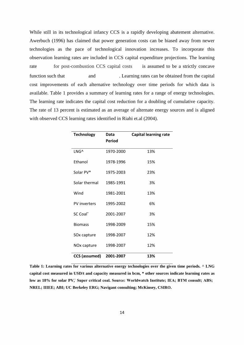
While still in its technological infancy CCS is a rapidly developing abatement alternative.
Awerbuch (1996) has claimed that power generation costs can be biased away from newer
technologies as the pace of technological innovation increases. To incorporate this
observation learning rates are included in CCS capital expenditure projections. The learning
rate for post-combustion CCS capital costs is assumed to be a strictly concave
function such that and . Learning rates can be obtained from the capital
cost improvements of each alternative technology over time periods for which data is
available. Table 1 provides a summary of learning rates for a range of energy technologies.
The learning rate indicates the capital cost reduction for a doubling of cumulative capacity.
The rate of 13 percent is estimated as an average of alternate energy sources and is aligned
with observed CCS learning rates identified in Riahi et.al (2004).
Technology Data Period
Capital learning rate
LNG^ 1970-2000 13%
Ethanol 1978-1996 15%
Solar PV* 1975-2003 23%
Solar thermal 1985-1991 3%
Wind 1981-2001 13%
PV inverters 1995-2002 6%
SC Coal˚ 2001-2007 3%
Biomass 1998-2009 15%
SOx capture 1998-2007 12%
NOx capture 1998-2007 12%
CCS (assumed) 2001-2007 13%
Table 1: Learning rates for various alternative energy technologies over the given time periods. ^ LNG
capital cost measured in USD/t and capacity measured in bcm, * other sources indicate learning rates as
low as 18% for solar PV, ̊ Super critical coal. Source: Worldwatch Institute; IEA; BTM consult; ABS;
NREL; IIIEE; ABI; UC Berkeley ERG; Navigant consulting; McKinsey, CSIRO.

15
A number of parameter assumptions were made to properly account for the energy penalty
during CO2 capture. We assume that type 2 (prior to 2015) and type 3 (after 2015) post-
combustion capture technologies were employed for retrofitting existing power plants. Type
2 and 3 post-combustion technologies are outlined in Riahi et.al. (2004) and we use the same
terminology for consistency. Type 2 and 3 technologies are advanced solvent-based solutions
with amines bases. We assume a capture rate of 90 percent, energy consumption of 300kWh/t
CO2 for capture and compression, capital expenditure for flue gas treatment of $17/t CO2 per
annum, capital expenditure of the capture plant of around $40/t CO2, reagent cost of $5/t CO2
and annual operating and maintenance costs equal to 4 percent of capital expenditure.
A complication for the Australian electricity coal fired generators is the general lack of NOx
and SOx control systems (flue gas desulphurisation or FGD), which means that either
solvents need to be developed which can be used economically with the current level of these
gases in the flue gases or an integrated approach be developed for emissions control. We
assume that the former will be the technology adopted as it is already well developed. The
latter solution will significantly improve the efficiency of the capture plant so our
conservative assumption will set a lower limit for emissions penalties.
The retrofit of type 2 and 3 technology will require sufficient space for a combined flue gas
cooler and de-SOx absorber. This study assumes that sufficient space is available at each of
the existing plants for retrofitting a capture and control system and in the majority of cases
there is ample room at each plant for a post-combustion CCS retrofit. Along with the energy
loss assumption for capture and compression, post-combustion capture also requires power to
operate solvent and cooling pumps, to cater for pressure losses in the FGD plant or CO2
absorber and for compression and liquefaction of the produced CO2 to pipeline pressure
(assumed at 100 bar). Energy loss assumptions are 0.04kWh/kg CO2 captured for pumps and
fans and 0.1kWh/kg CO2 captured for compression and liquefaction. Overall energy losses
average around 17 percent.
The McKinsey study assumes a weighted average cost of capital (WACC) of 8 percent which
is equivalent to the long-term bond rate plus 300 basis points (April 2008). This would be the
appropriate funding rate for a CCS plant funded through debt alone. The average debt-equity
ratio of Australia’s coal-fired power generators is around 1:1 implying a WACC at around 11
16
percent. We therefore use the higher WACC for this analysis as a conservative estimate for
capital costs.
For transportation and disposal it was assumed that the CO2 is transported in liquid state over
a distance of 100 km by pipe and stored in geological formations. We assume a cost for CO2
transportation at A$20/t CO2, which is based on estimates from the IEA (2006). This is about
50 percent higher than the costs assumed in the McKinsey study, which uses highly
interconnected CO2 sequestration in Europe as a baseline. The greater distance between
plants in Australia reduces the efficiency gained through an interconnected transport system
along with fewer locations with suitable geological conditions.
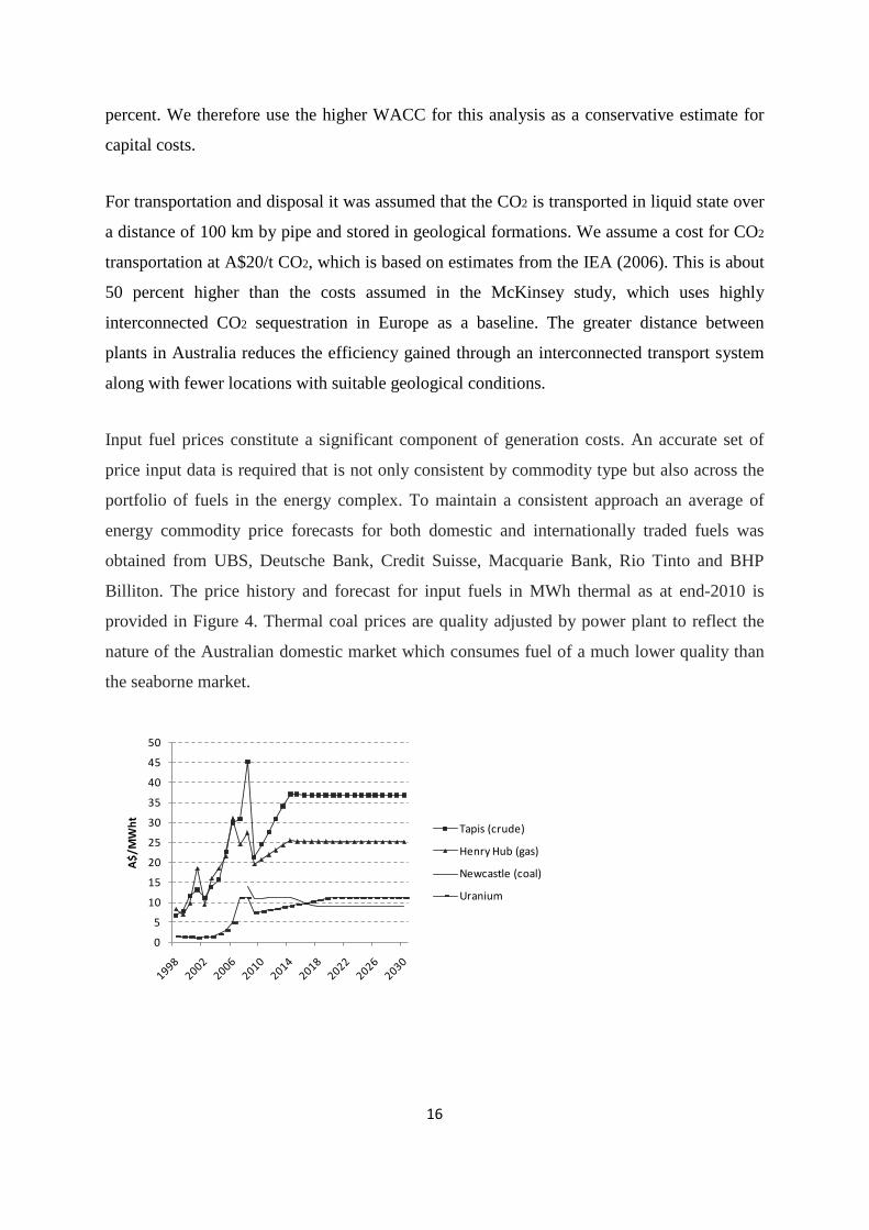
Input fuel prices constitute a significant component of generation costs. An accurate set of
price input data is required that is not only consistent by commodity type but also across the
portfolio of fuels in the energy complex. To maintain a consistent approach an average of
energy commodity price forecasts for both domestic and internationally traded fuels was
obtained from UBS, Deutsche Bank, Credit Suisse, Macquarie Bank, Rio Tinto and BHP
Billiton. The price history and forecast for input fuels in MWh thermal as at end-2010 is
provided in Figure 4. Thermal coal prices are quality adjusted by power plant to reflect the
nature of the Australian domestic market which consumes fuel of a much lower quality than
the seaborne market.
0
5
10
15
20
25
30
35
40
45
50
A$/
MW
ht Tapis (crude)
Henry Hub (gas)
Newcastle (coal)
Uranium
17
Figure 4: Price history and forecast of input fuels in MWh thermal (no adjustments for different plant
efficiencies) 2009-2030. Source: UBS, Deutsche Bank, Credit Suisse, Macquarie Bank, Rio Tinto and BHP
Billiton.
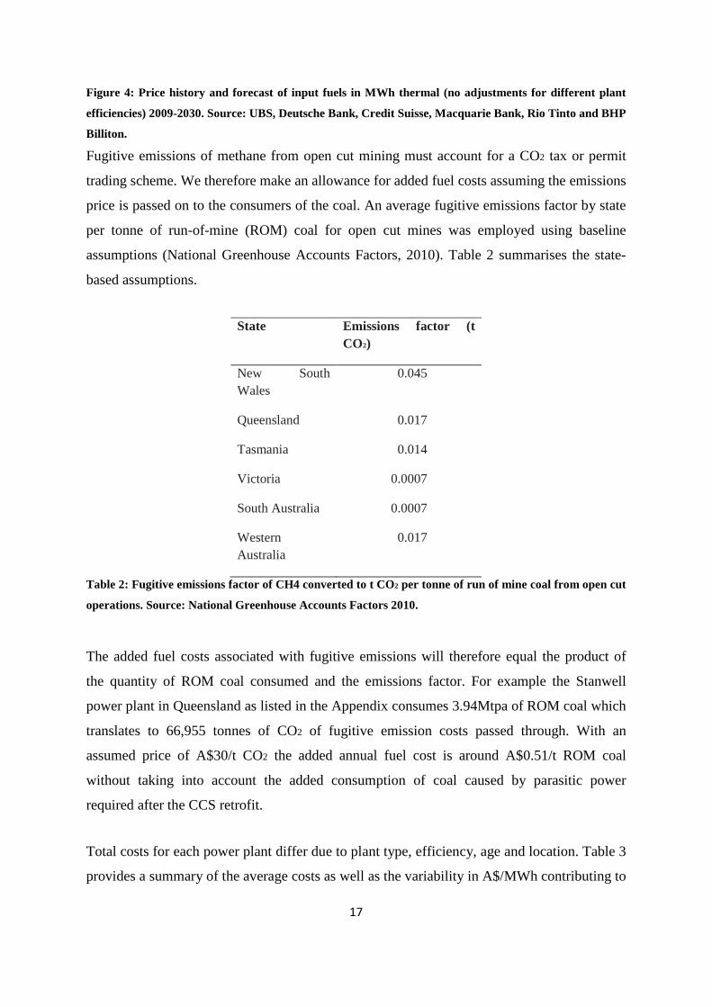
Fugitive emissions of methane from open cut mining must account for a CO2 tax or permit
trading scheme. We therefore make an allowance for added fuel costs assuming the emissions
price is passed on to the consumers of the coal. An average fugitive emissions factor by state
per tonne of run-of-mine (ROM) coal for open cut mines was employed using baseline
assumptions (National Greenhouse Accounts Factors, 2010). Table 2 summarises the state-
based assumptions.
State Emissions factor (t CO2)
New South Wales
0.045
Queensland 0.017
Tasmania 0.014
Victoria 0.0007
South Australia 0.0007
Western Australia
0.017
Table 2: Fugitive emissions factor of CH4 converted to t CO2 per tonne of run of mine coal from open cut
operations. Source: National Greenhouse Accounts Factors 2010.
The added fuel costs associated with fugitive emissions will therefore equal the product of
the quantity of ROM coal consumed and the emissions factor. For example the Stanwell
power plant in Queensland as listed in the Appendix consumes 3.94Mtpa of ROM coal which
translates to 66,955 tonnes of CO2 of fugitive emission costs passed through. With an
assumed price of A$30/t CO2 the added annual fuel cost is around A$0.51/t ROM coal
without taking into account the added consumption of coal caused by parasitic power
required after the CCS retrofit.
Total costs for each power plant differ due to plant type, efficiency, age and location. Table 3
provides a summary of the average costs as well as the variability in A$/MWh contributing to

18
the total cost associated with retrofitting CCS to existing plants. The total costs for the ‘no-
emissions’ price scenario excludes incremental operating and maintenance costs (including
reagent costs), additional fuel costs from fugitive emission cost pass-through, CO2 transport
and storage costs, unabated emissions costs and capital costs for CCS retrofit.
No emissions price
Average 10.13 11.36 0 0 0
Standard deviation
1.90 1.29 0 0 0
Emissions price
Average 26.74 12.01 20 2.14 39.25
Standard deviation
3.04 1.37 2 0.24 4.46
Table 3: Average component costs and standard deviations for CCS retrofit to existing coal-fired power
plants. CO2 costs are estimated since post-combustion capture and storage is assumed to abate 90 percent
of CO2 with the remainder incurring an emissions charge.
3.3. Real options and post-combustion CCS
The top-down approach requires an assumption around the timing of the installation of
abatement technologies. For instance the McKinsey top-down approach assumes a 10 percent
CCS retrofit to all coal-fired power plants in operation by 2020 (initially with the ones near
suitable geological features) and further assumes that two-thirds of all coal-fired power plants
in operation by 2030 employ CCS technology. These assumptions appear arbitrary and do not
quantitatively account for likely investment behaviour given the inherent value in investment
timing flexibility.
The real option value of an investment in CCS must include the strategic value of that
investment, along with the usual net present value (NPV) estimate. The real option value
is therefore
, (8)

19
where is the present value of the net revenue estimated over the life of the asset
and is the strategic value of the investment decision. Clearly the investment flexibility
in the timing of retrofitting a CCS plant may have positive value despite the NPV of the plant
having negative value. The technological immaturity of CCS and its installation as a retrofit
to coal-fired power plants is best viewed as an option to be exercised at an optimal time in the
future rather than as the central feature as an abatement option for consideration in the
present. Subsidised technology development can bring down the cost of CCS, but
commercially the technology will be just as unattractive at A$25/t CO2 as at A$125/t CO2 if
venting CO2 to the atmosphere remains free.
The lack of large scale demand for CO2 for enhanced oil recovery or other industrial uses for
CO2 in Australia, particularly near existing power stations, means that for a coal-fired power
station to retrofit CCS technology, it would only be considered as an alternative to paying a
tax on CO2 or decommissioning the plant. We therefore employ real options analysis to
determine if retrofitting CCS will increase the value of the power station using assumed
explicit prices for CO2 via either a tax or permit scheme.
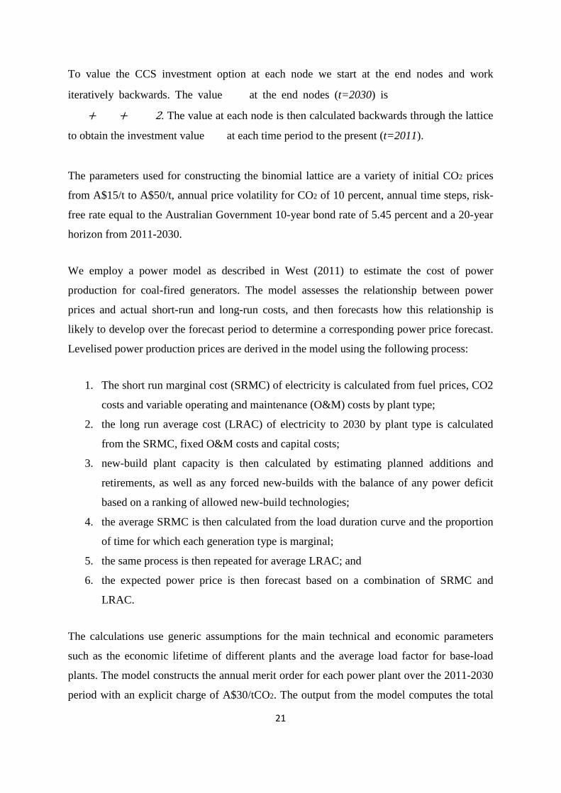
To value the strategic value of the timing for a CCS retrofit we employ a binomial lattice as it
is relatively simple to construct, allows for a variety of stochastic processes and jumps in
prices and it reflects the discrete annual investment option assessments conducted by power
producers willing to retrofit their plants with CCS technology.
To construct the binomial tree we commence with modelling the underlying CO2 price,
assuming the market for CO2 eventually reverts to prices based on a market mechanism. In its
simplest form, the diffusion approximation method assumes that the changes in the
investment value over time approximately follow a geometric Brownian motion (GBM)
diffusion process which is a standard assumption in finance literature (Cox, Ross and
Rubinstein, 1979; Hull, 2006). The price of CO2 either moves up by factor u or down by
factor d in period t+1. Factors u and d are linked to the volatility of the underlying emissions
price as
(9)

20
(10)
with risk-neutral probability
, (11)
where is the risk-free rate, is the annual volatility of the emissions price process and
is the time period between nodes. The argument supporting the risk neutral approach is that
since the valuation of options is based on arbitrage and is therefore independent of risk
preferences we can value the option assuming any set of risk preferences and arrive at the
same result. The value of each node in the tree is therefore derived as the expected value of
investment alternatives discounted at the risk-free rate
, (12)
where is the risk-neutral present value of the alternative investment options at time t+1.
Figure 5 illustrates the binomial lattice structure.
Figure 5: Three time periods of a simple binomial lattice. At each node the decision to retrofit or not
retrofit is made based on the value of the retrofit under a CO2 pricing regime where the combined costs
of capital and operating expenditures as well as the efficiency penalty are compared with the explicit CO2
price.
21
To value the CCS investment option at each node we start at the end nodes and work
iteratively backwards. The value at the end nodes (t=2030) is
+ + 2. The value at each node is then calculated backwards through the lattice
to obtain the investment value at each time period to the present (t=2011).
The parameters used for constructing the binomial lattice are a variety of initial CO2 prices
from A$15/t to A$50/t, annual price volatility for CO2 of 10 percent, annual time steps, risk-
free rate equal to the Australian Government 10-year bond rate of 5.45 percent and a 20-year
horizon from 2011-2030.
We employ a power model as described in West (2011) to estimate the cost of power
production for coal-fired generators. The model assesses the relationship between power
prices and actual short-run and long-run costs, and then forecasts how this relationship is
likely to develop over the forecast period to determine a corresponding power price forecast.
Levelised power production prices are derived in the model using the following process:
1. The short run marginal cost (SRMC) of electricity is calculated from fuel prices, CO2
costs and variable operating and maintenance (O&M) costs by plant type;
2. the long run average cost (LRAC) of electricity to 2030 by plant type is calculated
from the SRMC, fixed O&M costs and capital costs;
3. new-build plant capacity is then calculated by estimating planned additions and
retirements, as well as any forced new-builds with the balance of any power deficit
based on a ranking of allowed new-build technologies;
4. the average SRMC is then calculated from the load duration curve and the proportion
of time for which each generation type is marginal;
5. the same process is then repeated for average LRAC; and
6. the expected power price is then forecast based on a combination of SRMC and
LRAC.
The calculations use generic assumptions for the main technical and economic parameters
such as the economic lifetime of different plants and the average load factor for base-load
plants. The model constructs the annual merit order for each power plant over the 2011-2030
period with an explicit charge of A$30/tCO2. The output from the model computes the total
22
utilisation of each plant in the market for the assumed growth in demand and input costs. We
then employ the binomial lattice model to estimate the exercise date of the CCS retrofit
option assuming an emissions price of a known size commences in 2012.
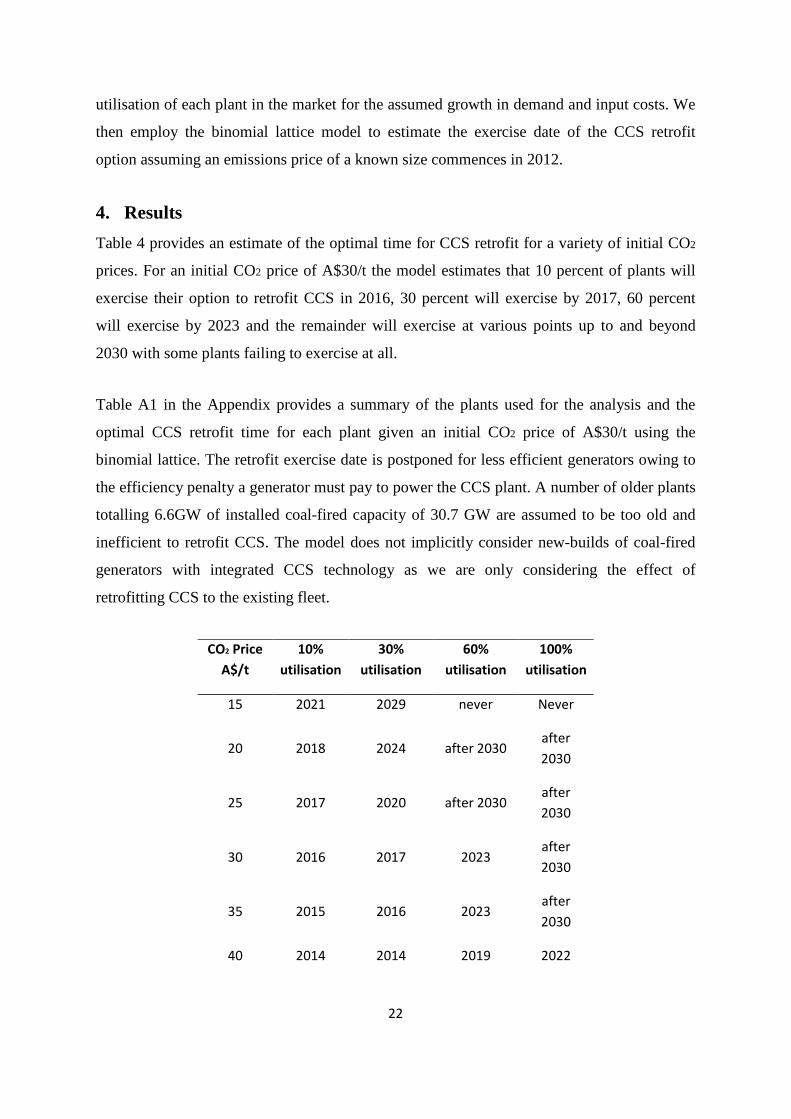
4. Results Table 4 provides an estimate of the optimal time for CCS retrofit for a variety of initial CO2
prices. For an initial CO2 price of A$30/t the model estimates that 10 percent of plants will
exercise their option to retrofit CCS in 2016, 30 percent will exercise by 2017, 60 percent
will exercise by 2023 and the remainder will exercise at various points up to and beyond
2030 with some plants failing to exercise at all.
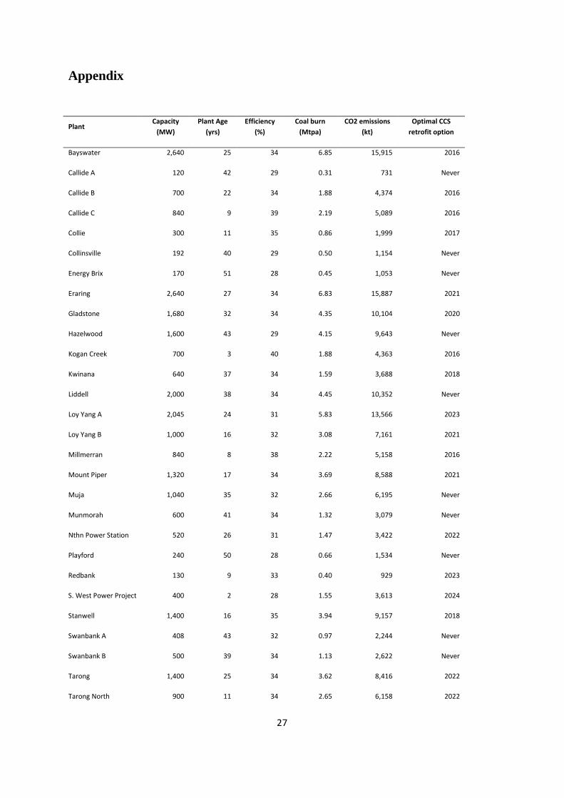
Table A1 in the Appendix provides a summary of the plants used for the analysis and the
optimal CCS retrofit time for each plant given an initial CO2 price of A$30/t using the
binomial lattice. The retrofit exercise date is postponed for less efficient generators owing to
the efficiency penalty a generator must pay to power the CCS plant. A number of older plants
totalling 6.6GW of installed coal-fired capacity of 30.7 GW are assumed to be too old and
inefficient to retrofit CCS. The model does not implicitly consider new-builds of coal-fired
generators with integrated CCS technology as we are only considering the effect of
retrofitting CCS to the existing fleet.
CO2 Price A$/t
10% utilisation
30% utilisation
60% utilisation
100% utilisation
15 2021 2029 never Never
20 2018 2024 after 2030 after 2030
25 2017 2020 after 2030 after 2030
30 2016 2017 2023 after 2030
35 2015 2016 2023 after 2030
40 2014 2014 2019 2022
23
45 2013 2013 2013 2013
50 2012 2012 2012 2012
Table 4: Utilisation rates to retrofit existing coal-fired power plants with CCS based on several CO2
prices.
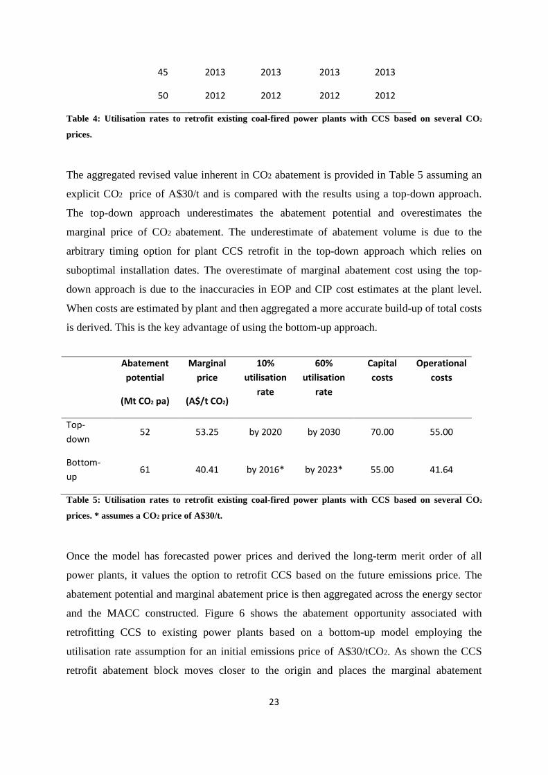
The aggregated revised value inherent in CO2 abatement is provided in Table 5 assuming an
explicit CO2 price of A$30/t and is compared with the results using a top-down approach.
The top-down approach underestimates the abatement potential and overestimates the
marginal price of CO2 abatement. The underestimate of abatement volume is due to the
arbitrary timing option for plant CCS retrofit in the top-down approach which relies on
suboptimal installation dates. The overestimate of marginal abatement cost using the top-
down approach is due to the inaccuracies in EOP and CIP cost estimates at the plant level.
When costs are estimated by plant and then aggregated a more accurate build-up of total costs
is derived. This is the key advantage of using the bottom-up approach.
Abatement potential
(Mt CO2 pa)
Marginal price
(A$/t CO2)
10% utilisation
rate
60% utilisation
rate
Capital costs
Operational costs
Top-down
52 53.25 by 2020 by 2030 70.00 55.00
Bottom-up
61 40.41 by 2016* by 2023* 55.00 41.64
Table 5: Utilisation rates to retrofit existing coal-fired power plants with CCS based on several CO2
prices. * assumes a CO2 price of A$30/t.
Once the model has forecasted power prices and derived the long-term merit order of all
power plants, it values the option to retrofit CCS based on the future emissions price. The
abatement potential and marginal abatement price is then aggregated across the energy sector
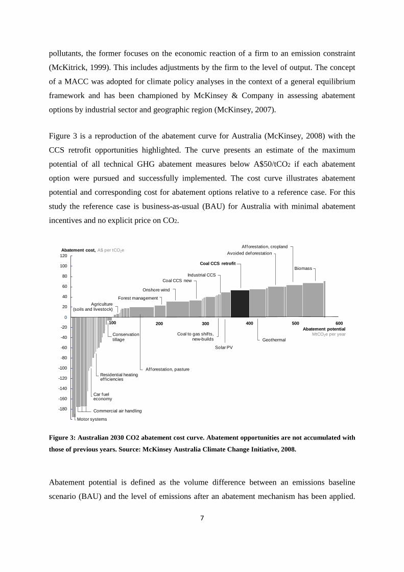
and the MACC constructed. Figure 6 shows the abatement opportunity associated with
retrofitting CCS to existing power plants based on a bottom-up model employing the
utilisation rate assumption for an initial emissions price of A$30/tCO2. As shown the CCS
retrofit abatement block moves closer to the origin and places the marginal abatement

24
opportunity for CCS retrofit ahead of other options such as solar PV and coal-to-gas shifts for
existing and new-builds. The cost of post-combustion CCS retrofit becomes comparable with
integrated pre-combustion CCS for newer plants using the bottom-up approach.
Figure 6: Australian 2030 CO2 abatement cost curve with post-combustion CCS retrofit using a bottom-
up model assuming a CO2 price of A$30/t.
Actual sequestration expenses are site-specific. While the improvement in CCS retrofit at the
margin is positive there are a number of competing CCS technologies such oxy-fuel and pre-
combustion which were not considered in this analysis. However the aggregated cost to
retrofit each of the pre-combustion technologies is likely to be of a similar scale to post-
combustion CCS out to 2030.
A variety of components are excluded from the abatement cost estimates. Some of these
factors could be included by adjusting one or more of the capital or operational cost elements
so that they act as a proxy for the ‘missing’ elements. Exogenous impacts such as the value of
government funded research programs, residual insurance responsibilities and external
pollution costs were explicitly ignored in the analysis. The system factors that were excluded
include transmission and other network costs, costs associated with providing energy
60
80
100
120
-20
-40
-60
40
200 300 400 500 6001000
20
-80
-100
-120
-140
-160
-180
Abatement cost, A$ per tCO2e
Motor systems
Commercial air handling
Geothermal
Solar PV
Coal CCS retrofit
Abatement potentialMtCO2e per year
Af forestation, pasture
Forest management
Onshore wind
Coal CCS new
Industrial CCS
Avoided deforestation
Biomass
Afforestation, cropland
Coal to gas shif ts, new-builds
Agriculture (soils and livestock)
Conservation tillage
Car fuel economy
Residential heating ef f iciencies
25
security, flexibility and management of power station output and the relative impact of
demand variation. The business impacts excluded from the model include the effect of
project size, scale and modularity, the fact that plant lifetime may exceed economic life, fuel
price volatility, regulatory changes and corporate taxes. The impact of a combination of these
factors could have some impact on abatement costs however estimating the probability of
such impacts, while difficult, is assumed to be immaterial for this analysis.
5. CONCLUSIONS Over a planning horizon, owners of electricity generating assets seek to minimise the net
present value (NPV) of future capital outlays, operating expenses and fuel costs. This
optimisation framework expands easily to accommodate an assessment of CCS retrofit costs.
Fundamentally CCS retrofit technologies compete with standard coal-fired generation plants
as an investment option and taxes on CO2 emissions and the costs of sequestration become
additional terms in the calculation of marginal operating costs. The MACC for the electricity
generation sector is derived using top-down NPV analysis and is a key decision tool used to
assess CCS retrofit investments.
The broad assumptions applied in constructing the MACC using a top-down approach result
in high marginal costs for CCS retrofit. However examination of the end-of-pipe and change-
in-process control technology costs for CCS retrofit on a generator-by-generator basis reveals
a marginal cost at a much lower resulting in feasible investment opportunities given an
explicit price on CO2 above A$30/t. Limitations associated with the top-down approach for
constructing abatement curves have been examined. Due to the weaknesses in this approach
we employ a bottom-up model to assess the marginal cost of retrofitting post-combustion
CCS plants to existing coal-fired generators. The bottom-up approach accounts for plant
variations in efficiency and efficiency penalties after CCS retrofit, CO2 intensity levels,
diminishing capital costs through learning and added fuel costs from fugitive emissions. A
binomial option pricing model was used to estimate the timing of each plant’s CCS retrofit
based on an assumed emissions price. Application of policy centred solely on the results from
the top-down approach to measure marginal abatement can result in decisions that are in
danger of dismissing the valuable option to retrofit CCS to coal-fired generators. If CCS
technology fails to manifest in the power sector and its potential contribution is replaced by

26
renewable energy sources the modelling indicates that the economic cost of abatement is
likely to rise significantly.
27
Appendix
Plant Capacity
(MW) Plant Age
(yrs) Efficiency
(%) Coal burn
(Mtpa) CO2 emissions
(kt) Optimal CCS
retrofit option
Bayswater 2,640 25 34 6.85 15,915 2016
Callide A 120 42 29 0.31 731 Never
Callide B 700 22 34 1.88 4,374 2016
Callide C 840 9 39 2.19 5,089 2016
Collie 300 11 35 0.86 1,999 2017
Collinsville 192 40 29 0.50 1,154 Never
Energy Brix 170 51 28 0.45 1,053 Never
Eraring 2,640 27 34 6.83 15,887 2021
Gladstone 1,680 32 34 4.35 10,104 2020
Hazelwood 1,600 43 29 4.15 9,643 Never
Kogan Creek 700 3 40 1.88 4,363 2016
Kwinana 640 37 34 1.59 3,688 2018
Liddell 2,000 38 34 4.45 10,352 Never
Loy Yang A 2,045 24 31 5.83 13,566 2023
Loy Yang B 1,000 16 32 3.08 7,161 2021
Millmerran 840 8 38 2.22 5,158 2016
Mount Piper 1,320 17 34 3.69 8,588 2021
Muja 1,040 35 32 2.66 6,195 Never
Munmorah 600 41 34 1.32 3,079 Never
Nthn Power Station 520 26 31 1.47 3,422 2022
Playford 240 50 28 0.66 1,534 Never
Redbank 130 9 33 0.40 929 2023
S. West Power Project 400 2 28 1.55 3,613 2024
Stanwell 1,400 16 35 3.94 9,157 2018
Swanbank A 408 43 32 0.97 2,244 Never
Swanbank B 500 39 34 1.13 2,622 Never
Tarong 1,400 25 34 3.62 8,416 2022
Tarong North 900 11 34 2.65 6,158 2022

28
Vales Point B 1,320 32 34 3.41 7,936 2022
Wallerawang C 1,000 32 34 2.59 6,014 2022
Yallourn West 1,450 32 31 4.01 9,317 2023
Total 30,735 - - 81.49 189,461 -
Average - 27 33 - - -
Table A1: Coal-fired plants used for bottom-up marginal abatement curve construction. Retrofit column
indicates optimal time to retrofit CCS based on CO2 prices of A$30/t.
29
References Awerbuch, S. (1996) Capital budgeting, technological innovation and the emerging
competitive environment of the electric power industry, Energy Policy 24 (2), 195-202.
Beaumont, N.J. and Tinch, R. (2004) Abatement cost curves: a viable management tool for
enabling the achievement of win–win waste reduction strategies? Journal of Environmental
Management 71, 207-215.
Coggins, J.S. and Swinton, J.R. (1996) The price of pollution: a dual approach to valuing
SO2 allowances, Journal of Environmental Economics and Management 30, 58-72.
Cox, J.C., Ross, S.A. and Rubinstein, M. (1979) Option pricing: A simplified approach,
Journal of Financial Economics 7, 229-263.
Fare, R., Grosskopf, S., Lovell, C.A.K., and Yaisawarng, S. (1993) Derivation of shadow
prices for undesirable outputs: a distance function approach, Review of Economics and
Statistics 75, 374-380.
Gollop, F.M. and Roberts, M.J. (1985) Cost-minimizing regulation of sulphur emissions:
regional gains in electric power, Review of Economics and Statistics 67, 81-90.
Hull, J. (2006) Options, Futures and Other Derivatives, Prentice Hall, New Jersey.
International Energy Agency (IEA). (2009) World Energy Outlook, Paris, OECD.
Johnson, T.L. (2002) Electricity without carbon dioxide: assessing the role of carbon capture
and sequestration in US electric markets, PhD thesis, Department of Engineering and Public
Policy, Carnegie Mellon University, Pittsburgh, 266.
Karvosenoja, N. and Johansson, M. (2003) Cost curve analysis for SO2 and NOx emission
control in Finland, Environmental Science and Policy 6, 329-340.
Klepper, G. and Peterson,S. (2006) Marginal abatement cost curves in general equilibrium:
the influence of world energy prices, Resource and Energy Economics 28, 1-23.
30
Lee, J.-D., Park, J.-B. and Kim,T.-Y. (2002) Estimation of the shadow prices of pollutants
with production/environment inefficiency taken into account: a non parametric directional
distance function approach, Journal of Environmental Management 64, 365-375.
Lee, M. (2005) The shadow price of substitutable sulphur in the US electric power plant: a
distance function approach, Journal of Environmental Management 77, 104-110.
McKinsey & Company (2007) Pathways to a low carbon economy, McKinsey & Company.
McKinsey & Company (2008) An Australian cost curve for greenhouse gas reduction,
McKinsey Australia Climate Change Initiative, Sydney.
McKitrick, R. (1999) A derivation of the marginal abatement cost curve, Journal of
Environmental Economics and Management 37, 306-314.
National Greenhouse Accounts Factors (2010) Department of Climate Change and Energy
Efficiency, Australian Government, Canberra, ACT.
Riahi, K., Rubin, E.S., Taylor, M.R., Schrattenholzer, L. and Hounshell, D. (2004)
Technological learning for carbon capture and sequestration technologies, Energy Economics
26, 539-564.
Rubin, E.S., Rao, A.B. and Berkenpas, M.B. (2001) A multi-pollutant framework for
evaluating CO2 control options for fossil fuel power plants. Proceedings of First National
Conference on Carbon Sequestration, US Department of Energy, Washington, DC.
West, J.M. (2011) Picking winners: Understanding the future cost of energy generation in
Australia, JASSA: The Finsia Journal of Applied Finance 1, 13-19.
Weyant, J. (1999) The costs of the Kyoto Protocol: a multi-model evaluation, The Energy
Journal, Special Issue.
Recommended