University of New MexicoUNM Digital Repository
Civil Engineering ETDs Engineering ETDs
2-14-2014
Material Characteristics of Hot Mix Asphalt andBinder Using Freeze-Thaw ConditioningGhazanfar Barlas
Follow this and additional works at: https://digitalrepository.unm.edu/ce_etds
This Thesis is brought to you for free and open access by the Engineering ETDs at UNM Digital Repository. It has been accepted for inclusion in CivilEngineering ETDs by an authorized administrator of UNM Digital Repository. For more information, please contact [email protected].
Recommended CitationBarlas, Ghazanfar. "Material Characteristics of Hot Mix Asphalt and Binder Using Freeze-Thaw Conditioning." (2014).https://digitalrepository.unm.edu/ce_etds/88

i
Ghazanfar Barlas Candidate
Civil Engineering
Department
This thesis is approved, and it is acceptable in quality and form for publication:
Approved by the Thesis Committee:
Dr. Rafiqul A. Tarefder, Chairperson
Dr. Arup K. Maji
Dr. Mahmoud Reda Taha
ii
MATERIAL CHARACTERISTICS OF HOT MIX ASPHALT
AND BINDER
USING FREEZE-THAW CONDITIONING
by
GHAZANFAR BARLAS
B.S., CIVIL ENGINEERING
UNIVERSITY OF NEW MEXICO
THESIS
Submitted in Partial Fulfillment of the
Requirements for the Degree of
Master of Science
Civil Engineering
The University of New Mexico
Albuquerque, New Mexico
December, 2013

iii
DEDICATIONS
I would like to dedicate my work to my parents. My mother, who supported me in every
step of life but unfortunately could not fight the battle of cancer. My father has been my
motivation for pursuing a career in Civil Engineering.
iv
ACKNOWLEDGMENTS
First and foremost, I would like to thank my parents, Shafiqa Ahmadi and Muhammad
Nadir Ahmadi, who have supported me spiritually throughout my life and during my
studies. Next, I would like to thank Professor Rafiqul A. Tarefder, my advisor, for his
support and guidance during the time of my research. I would also like to thank Professor
Arup K. Maji and Professor Mahmoud Reda Taha for their valuable time and being the
members of my thesis committee. Also, I would like to thank the New Mexico
Department of Transportation for their support: Jeff Mann (Head of Pavement Design,
NMDOT), Parveez Anwar (State Asphalt Engineer, NMDOT), and Virgil Valdez
(Research Bureau, NMDOT) for their valuable suggestions and continuous support. I
owe my utmost gratitude to Hasan M. Faisal for his laboratory assistance, data analysis,
and continuous support throughout my study. I would like to thank Md Rashadul Islam
for his help and discussions. Lastly, I would like to thank my family, friends, and
colleagues for their support during the completion of my thesis.

v
MATERIAL CHARACTERISTICS OF HOT MIX ASPHALT
AND BINDER
USING FREEZE-THAW CONDITIONING
by
Ghazanfar Barlas
B.S., Civil Engineering, University of New Mexico, 2011
M.S., Civil Engineering, University of New Mexico, 2013
ABSTRACT
Depending on the region, in a single year, the pavement undergoes many cycles of
freezing and thawing. Freeze-thaw, as well as traffic loading, are important parameters in
the study of damage in asphalt pavement. In areas of wide ranging temperatures,
pavements are susceptible due to thermal cracking. This study investigates the effect of
freeze-thaw on fatigue life and material characteristics of Hot Mix Asphalt (HMA) and
binder. Since, temperature is variable throughout the year, a constant temperature should
not be assumed when finding the fatigue life and material characteristics of HMA. To
evaluate the damage, flexure test is conducted to determine the effect of freeze-thaw on
the modulus and the fatigue life. In concurrence with the flexure test, indirect tensile
(IDT) strength test is performed on the same mix with similar freeze-thaw conditioning to
determine the reduction in the strength of HMA. Furthermore, Bending Beam Rheometer
(BBR) test is performed on the binder that is used for the HMA. Similarly, the binder is
vi
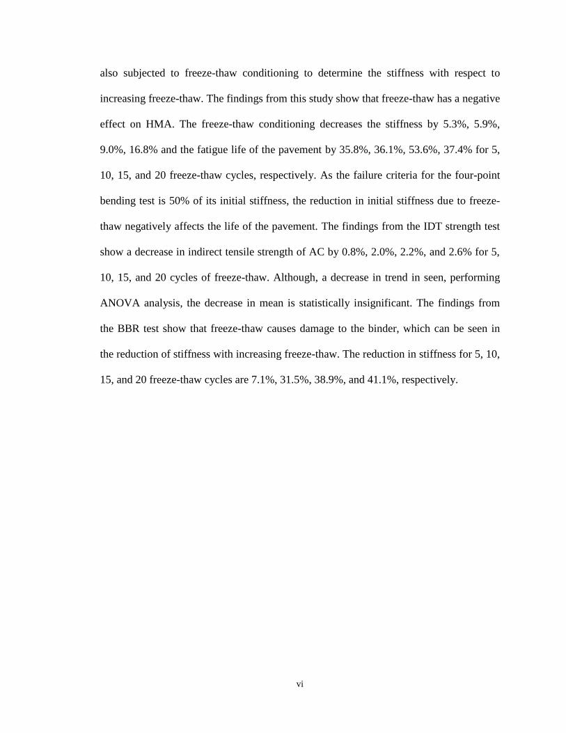
also subjected to freeze-thaw conditioning to determine the stiffness with respect to
increasing freeze-thaw. The findings from this study show that freeze-thaw has a negative
effect on HMA. The freeze-thaw conditioning decreases the stiffness by 5.3%, 5.9%,
9.0%, 16.8% and the fatigue life of the pavement by 35.8%, 36.1%, 53.6%, 37.4% for 5,
10, 15, and 20 freeze-thaw cycles, respectively. As the failure criteria for the four-point
bending test is 50% of its initial stiffness, the reduction in initial stiffness due to freeze-
thaw negatively affects the life of the pavement. The findings from the IDT strength test
show a decrease in indirect tensile strength of AC by 0.8%, 2.0%, 2.2%, and 2.6% for 5,
10, 15, and 20 cycles of freeze-thaw. Although, a decrease in trend in seen, performing
ANOVA analysis, the decrease in mean is statistically insignificant. The findings from
the BBR test show that freeze-thaw causes damage to the binder, which can be seen in
the reduction of stiffness with increasing freeze-thaw. The reduction in stiffness for 5, 10,
15, and 20 freeze-thaw cycles are 7.1%, 31.5%, 38.9%, and 41.1%, respectively.
vii
Table of Contents CHAPTER 1 .................................................................................................................................................... 1
INTRODUCTION ........................................................................................................................................... 1
1.1. Problem Statement ...................................................................................................................... 1
1.1 Hypothesis .................................................................................................................................... 3
1.1.1 Hypothesis 1 .............................................................................................................................. 3
1.1.2 Hypothesis 2 .............................................................................................................................. 3
1.2 Outline .......................................................................................................................................... 4
CHAPTER 2 .................................................................................................................................................... 5
LITERATURE REVIEW ................................................................................................................................ 5
2.1 Introduction .................................................................................................................................. 5
2.2 Current and Past Studies on Freeze-Thaw Conditioning Methods ......................................... 5
2.3 Freeze-Thaw Conditioning Approaches .................................................................................. 10
2.4 Four-Point Bending Test ........................................................................................................... 11
2.5 Indirect Tensile Strength Test .................................................................................................. 12
2.6 Bending Beam Rheometer Test ................................................................................................ 13
2.7 Remarks ...................................................................................................................................... 14
CHAPTER 3 .................................................................................................................................................. 15
SAMPLE PREPARATION AND LABORATORY TESTING ................................................................... 15
3.1 Experimental Plan ..................................................................................................................... 15
3.2 HMA Mixture Gradation .......................................................................................................... 15
3.3 Sample Preparation ................................................................................................................... 17
3.3.1 Beam Specimen ....................................................................................................................... 17
3.3.2 Cylindrical Specimen .............................................................................................................. 19
3.3.3 BBR Specimen ........................................................................................................................ 21
3.4 Sample Cutting ........................................................................................................................... 23
3.4.1 Asphalt Beam Samples ............................................................................................................ 23
3.4.2 Asphalt Cylinder Samples ....................................................................................................... 25
3.5 Specimen Volumetric Analysis ................................................................................................. 26
3.6 Sample Conditioning ................................................................................................................. 27
3.7 Four-Point Bending Test ........................................................................................................... 29
3.8 Indirect Tensile Strength Test .................................................................................................. 32
3.9 Bending Beam Rheometer Test ................................................................................................ 35
CHAPTER 4 .................................................................................................................................................. 38
EFFECT OF FREEZE-THAW ON BEAM FATIGUE PARAMETERS ..................................................... 38
4.1 Introduction ................................................................................................................................ 38
4.2 Fatigue Test ................................................................................................................................ 39
4.2.1 Results and Discussion on Beam Fatigue Test ........................................................................ 39
CHAPTER 5 .................................................................................................................................................. 54
viii
EFFECTS OF FREEZE-THAW ON INDIRECT TENSILE STREGNTH AND BENDING BEAM
RHEOMETER STIFFNESS ......................................................................................................................... 54
5.1 Introduction ................................................................................................................................ 54
5.2 Indirect Tensile Strength Test .................................................................................................. 56
5.2.1 Results and Discussion for IDT Test ....................................................................................... 56
5.3 Bending Beam Rheometer Test ................................................................................................ 62
5.3.1 Results and Discussion for BBR Test ...................................................................................... 62
CHAPTER 6 .................................................................................................................................................. 71
CONCLUSIONS AND RECOMMENDATIONS ........................................................................................ 71
6.1 Conclusions ................................................................................................................................. 71
6.1.1 Fatigue Test Conclusion .......................................................................................................... 71
6.1.2 IDT Test Conclusion ............................................................................................................... 72
6.1.3 BBR Test Conclusion .............................................................................................................. 73
6.2 Recommendations for Future Work ........................................................................................ 73
REFERNCES ................................................................................................................................................ 74
ix
LIST OF FIGURES
Figure 3.1: Aggregate Gradation for SP-III Mixture ..................................................................................... 16
Figure 3.2: Linear Kneading Compactor ....................................................................................................... 18
Figure 3.3: Linear Kneading Compactor Mold ............................................................................................. 18
Figure 3.4: Pine Gyratory Compactor ........................................................................................................... 20
Figure 3.5: Molded Sample with 8 inches Height and 6 inches Diameter .................................................... 20
Figure 3.6: Trimming of Room Temperature Binder Sample ....................................................................... 21
Figure 3.7: Finished BBR sample ................................................................................................................. 22
Figure 3.8: Finished sample conditioning of Binder Sample in -10°C .......................................................... 22
Figure 3.9: Uncut Hot Mix Asphalt Beam Samples ...................................................................................... 23
Figure 3.10: GCTS stone-cutting saw with original clamps .......................................................................... 24
Figure 3.11: GCTS stone-cutting saw with modified clamps ........................................................................ 24
Figure 3.12: GCTS Pressure Controlled Core Drill....................................................................................... 25
Figure 3.13: Espec Temperature/Humidity Chamber .................................................................................... 28
Figure 3.14: Samples Being Conditioned by Freeze-Thaw Method.............................................................. 28
Figure 3.15: Typical Four-Point Bending Test Schematic ............................................................................ 29
Figure 3.16: GCTS Flexural Beam Setup ...................................................................................................... 31
Figure 3.17: Beam Fatigue Test Setup with the LVDT Attached.................................................................. 31
Figure 3.18: IDT Sample with Dimensions ................................................................................................... 33
Figure 3.19: IDT Asphalt Concrete Sample .................................................................................................. 33
Figure 3.20: IDT Test Setup with a Specimen .............................................................................................. 34
Figure 3.21: BBR Sample with Dimensions ................................................................................................. 36
Figure 3.22: BBR Testing Apparatus ............................................................................................................ 36
Figure 3.23: BBR Test Setup with a Sample ................................................................................................. 37
Figure 4.1: Stiffness versus Different Numbers of Freeze-Thaw Cycles Curve ........................................... 40
Figure 4.2: Comparison of Number of Cycles to Failure with Different Freeze-Thaw Cycles ..................... 41
Figure 4.3: Comparison of Stiffness Reduction with Different Freeze-Thaw Cycles ................................... 42
Figure 4.4: Stiffness versus Number of Cycles for 0 Freeze-Thaw Cycles ................................................... 44
Figure 4.5: Stiffness versus Number of Cycles for 5 Freeze-Thaw Cycles ................................................... 44
Figure 4.6: Stiffness versus Number of Cycles for 10 Freeze-Thaw Cycles ................................................. 45
Figure 4.7: Stiffness versus Number of Cycles for 15 Freeze-Thaw Cycles ................................................. 45
Figure 4.8: Stiffness versus Number of Cycles for 20 Freeze-Thaw Cycles ................................................. 46
Figure 4.9: Stiffness Ratio versus Number of Cycles for 0 Freeze-Thaw Cycles ......................................... 47
Figure 4.10: Stiffness Ratio versus Number of Cycles for 5 Freeze-Thaw Cycles ....................................... 47
Figure 4.11: Stiffness Ratio versus Number of Cycles for 10 Freeze-Thaw Cycles ..................................... 48
Figure 4.12: Stiffness Ratio versus Number of Cycles for 15 Freeze-Thaw Cycles ..................................... 48
x
Figure 4.13: Stiffness Ratio versus Number of Cycles for 20 Freeze-Thaw Cycles ..................................... 49
Figure 4.14: Correlation of Initial Stiffness with Increasing Number of F-T Cycles .................................... 50
Figure 4.15: Box Plot for Different Cycles of F-T with Their Respective Initial Stiffness ........................... 51
Figure 4.16: Correlation of Number of Cycles to Failure to F-T Cycles ....................................................... 52
Figure 4.17: Box Plot for No. of Cycles to Failure with Respective F-T Cycles .......................................... 53
Figure 5.1: Comparison of IDT Strength with different Freeze-Thaw Cycles .............................................. 59
Figure 5.2: Strength Reduction with Different Freeze-Thaw Cycles ............................................................ 59
Figure 5.3: Comparison of Tensile Strength Ratio with different Freeze-Thaw Cycles ............................... 60
Figure 5.4: Box Plot for IDT Strength with Respective F-T Cycles ............................................................. 61
Figure 5.5: Test Data Plot Obtained for Asphalt Binder for 20 cycles of F-T............................................... 63
Figure 5.6: Displacement over Time for 0 F-T Cycles .................................................................................. 64
Figure 5.7: Displacement over Time for 5 F-T Cycles .................................................................................. 64
Figure 5.8: Displacement over Time for 10 F-T Cycles ................................................................................ 65
Figure 5.9: Displacement over Time for 15 F-T Cycles ................................................................................ 65
Figure 5.10: Displacement over Time for 20 F-T Cycles .............................................................................. 66
Figure 5.11: Stiffness with Respect to Freeze-Thaw Cycles ......................................................................... 66
Figure 5.12: plot of stiffness vs. logarithmic time for m-value calculation for 60 sec. ................................. 68
Figure 5.13: Box Plot for different cycles of F-T with their respective Stiffness.......................................... 68
Figure 5.14: m-value Box Plot for Each Class of Freeze-Thaw Cycle .......................................................... 69
xi
LIST OF TABLES
Table 3.1: Aggregate Gradation for SP-III .................................................................................................... 16
Table 4.1: Fatigue Test Results with Different Cycles of Freeze-Thaw ........................................................ 42
Table 5.1: Test Matrix for IDT Test .............................................................................................................. 55
Table 5.2: Test Matrix for Bending Beam Rheometer Test .......................................................................... 55
Table 5.3: Laboratory Indirect Tensile Strength and Tensile Strength Ratio ................................................ 57
Table 5.4: Stiffness and m-value Test Results for BBR ................................................................................ 70

1
1 CHAPTER 1
INTRODUCTION
1.1. Problem Statement
Hot Mix Asphalt (HMA) in pavement structures has been used throughout United States
and worldwide. As more research is being done, there have been significant changes in
the way pavements are built today. Design standards are constantly updated and changing
with new ways of analyzing and predicting the behavior of HMA. Pavements are built
with several criteria in mind and depending on the location of the pavement, different
mix designs, traffic intensity, and climatic factors are taken into consideration.
The design of asphalt pavements mainly focuses on resisting rutting, low temperature
cracking, and fatigue cracking. With the use of Performance Grade (PG) binders, the
rutting issue can be addressed on the binder level. Climate plays a major role in traffic
induced fatigue and low-temperature cracking. Pavement experiences various weather
conditions as well as high intensity traffic loading over a certain period of time.
Consequently, the latest testing in time dependent testing of asphalt is needed, along with
a similar weathering condition. One of the common weather patterns a pavement
experiences is freezing and thawing. Kestler et al, (2011) found that there is a correlation
between the fatigue damage (Asphalt Institute) and winter season weather pattern.
Statistical study indicated that more fatigue damage occurs in shorter winters as well as
warmer winters with shallow freeze-thaw depths. To address this issue, the use of freeze-
thaw conditioning is recommended to represent the field conditions.

2
Freeze-thaw damage, as well as traffic loading, are important parameters in life of asphalt
pavement. As the weather is not constant throughout the year, it gets cold in the winter
and hot in the summer, it is not feasible to assume a constant temperature when trying to
find the fatigue life and material characteristics of HMA. Depending on the region, in a
single year, the pavement undergoes many cycles of freezing and thawing (Goh and You
2012; Attia and Abdelrahman 2010; Loria et al, 2011; Bolzan 1989; Ozgan and Serin
2012; Feng et al, 2010; Chen and Huang 2007; Lu and Harvey 2008). Some researchers
have shown, through indirect tensile test, that after each cycle of freezing and thawing,
the tensile strength ratio decreases (Chen and Huang 2007; Feng et al, 2010; Shu et al,
2012; Loria et al, 2011).
In 2010, Mei et al, researched the fatigue life of asphalt pavement and in the study,
splitting fatigue test was performed. The two major drawbacks of this study was there
was no comparison between several freeze-thaw cycles and of lately, most researchers
use four-point bending tests to determine the fatigue life of asphalt pavements because of
its ability to better predict fatigue life. A study needs to be conducted on the effects of
freeze-thaw cycles on asphalt pavement through the use four-point bending test to
understand its effect on pavement life. Another objective of this thesis is to relate the
asphalt binder’s creep stiffness as a function of time and also perform indirect tensile
strength of asphalt concrete when it has been subjected to freeze-thaw cycles.
3
1.1 Hypothesis
1.1.1 Hypothesis 1
Although in the previous research, it is shown that freeze-thaw has a negative effect on
the engineering properties of asphalt, strength of asphalt samples have shown to decrease.
Little to no work has been done to find the effect of freeze-thaw on the fatigue life and
stiffness of asphalt material. It hypothesized that the same negative effect may occur on
the fatigue life and stiffness of asphalt as well. This hypothesis can be proven by inducing
freeze-thaw conditioning and performing four-point bending test on asphalt samples and
Bending Beam Rheometer test on the binder.
1.1.2 Hypothesis 2
In previous research, done on the strength of asphalt, it has been shown that most damage
occurs during the first stages of freeze-thaw and then deceases steadily with every cycle
of freeze-thaw. It can be hypothesized that same damage trend may occur for local NM
mixes. The fatigue life will be affected the most with the first freeze-thaw conditioning
and decrease slowly. An equation can be developed which can relate damage of asphalt
with the number of freeze-thaw cycles. Moreover, from the initial stiffness of asphalt, a
prediction can be made to determine the stiffness of the pavement after a given number of
freeze-thaw cycles. Furthermore, the results from IDT tests may support the findings of
the fatigue tests. A model can be created to describe the damage occurring after freeze-
thaw for the IDT test.
4
1.2 Outline
In this study, the effect of freeze-thaw conditioning on the HMA and binder is
introduced. Freeze-thaw conditioning is used in conjunction with four-point bending test,
indirect tensile strength test, and bending beam rheometer test.
This thesis will include 6 chapters: Introduction, literature review, sample preparation
and laboratory testing, effect of freeze-thaw on beam fatigue parameters, effect of freeze-
thaw on indirect tensile strength and bending beam rheometer stiffness, and Conclusion.
Chapter Two, the literature review, summarizes moisture damage (freeze-thaw) to
asphalt and their relations to the present study.
Chapter Three, sample preparation and laboratory testing, describes the
experimental plan for this study. This chapter includes material selection, sample
preparation, sample conditioning, laboratory fatigue testing, indirect tensile strength
testing and bending beam rheometer testing.
Chapter Four, effect of freeze-thaw on beam fatigue parameters, will include the
laboratory data and analysis which has been obtained from the freeze-thaw conditioning.
Chapter Five, effect of freeze-thaw on indirect tensile test and bending beam
rheometer test, will include the laboratory data and analysis which has been obtained
from the freeze-thaw conditioning.
Chapter Six is the concluding chapter for this study. This chapter summarizes the
findings from the laboratory tests with freeze-thaw conditioning.
5
2 CHAPTER 2
LITERATURE REVIEW
2.1 Introduction
This chapter presents a summary of moisture induced freeze-thaw conditioning of asphalt
material and its relevant testing methods by previously conducted and on-going research.
2.2 Current and Past Studies on Freeze-Thaw Conditioning Methods
Moisture Damage is one of the major concerns in asphalt pavements. Moisture damage
can be described in two different stages, loss of adhesion and loss of cohesion. Loss of
adhesion, which is the stripping of asphalt film, occurs between the asphalt and the
aggregate. This phenomenon is called “stripping”. Loss of cohesion happens within the
binder itself due to water infiltration and causes a loss of mixture stiffness, which a
complex phenomenon affected by many factors.
Moisture related damage can be attributed by a lot of distresses in pavement. Some of the
factors the can contribute to moisture related distress are the mix design (binder type,
binder content, aggregate, air voids, and additives), production of the Hot Mix Asphalt
(HMA), Construction (compaction, permeability, reproducibility), and most importantly
Climate (freeze-thaw, rainfall, excessive heat). Some other factors which affect the life
and durability of asphalt pavements are surface drainage, subsurface drainage, rehab
strategies and truck volume).
Asphalt is a viscoelastic material, which means it can heal if given enough time. Cracks
in the pavement occur due to many climatic, traffic, and construction reasons. The major
reason as to why pavement collapse fail at a faster rate is the repeated truck traffic and
6
freeze-thaw cycles (Garcia, 2011). Garcia found that the healing rates of asphalt mastic
increases with the increase of temperature. Although, it is possible for the asphalt mastic
to heal, it is complex to predict the healing time and temperature which is a function of
the aging and the binder type.
There are limited researches dedicated to the study of freeze-thaw on asphalt pavement.
Work by Feng et al., 2009 showed that freeze-thaw damage occurs in three different
stages. Feng concluded that with the increase of freeze-thaw cycles, the splitting strength
of asphalt decreased, weight loss rate decreased while the volume of the mix expanded in
a steady manner. Feng also noted that the performance stabilized until the next rapid
deterioration caused by loss of adhesion. Indirect tensile strength tests were performed at
0, 2, 4, 6, 8 cycles of freeze-thaw conditioning. However, to understand the behavior of
the pavement, a fatigue test is required to capture the deterioration over a number of
years.
Mei et al., 2010 at Jiaotong University in China reported that fatigue life of asphalt
pavements in rich rainfall areas are about 60% of that in a drought or little rain area. It
was also noticed that the better fatigue life was observed as the pavement thickness
increased. This of course will lead to a higher pavement cost which is not plausible. Mei
adopted the test method of split fatigue test which uses a stress controlled method to
define the fatigue life. Stress controlled method is acceptable when the thickness of the
pavement is greater than 5 inches (125 mm). With the use of different pavement design
methods, more pavement are designed with different layers and most asphalt layer close
to the top surface have a thickness of less than 5 inches. Since the most damage occurs
7
towards the top, constant strain test would yield a more accurate representation of the
pavement life.
In another study by Feng et al., 2010, which relates the impact of salt versus distilled
water with the conditioning method of freeze-thaw, it was found that freeze-thaw damage
of asphalt mixtures include two phases. In first phase, the damage is caused by the
expansion of water which would ultimately decrease the indirect tensile strength of the
asphalt. The damage of the second phase occurs on the interfacial of the mix between the
asphalt and the aggregate or in some cases, the fracture of asphalt mortar which results in
weight loss. It was also found that salt plays a major role in the low temperature
performance of asphalt binder. Particularly, when the percentage of salt is greater than 3,
the deformability of asphalt decreases rapidly. However, no attempt was done in this
study to relate the fatigue life of the pavement.
While in an attempt to figure out the effect of freeze-thaw on the fatigue life of asphalt,
other researcher have investigated certain engineering characteristics of asphalt being
exposed to freeze-thaw conditioning. Ozgan and Serin (2012) investigated effect of
freeze-thaw on the binder and wearing surface coats. In this particular study, specimens
were exposed to freeze-thaw cycles for 6, 12, 18, and 24 days after which the voids ratios
fill with asphalt, void ratio, and the voids ratios inside the aggregate were determined by
the method of ultrasonic velocity and Marshall Stability. Ultrasonic Velocity is a test
done on materials to measure their acoustic velocity in order to measure some mechanical
properties. The findings from the research concluded that there are important negative
effects of the freeze-thaw on the engineering properties of asphalt mixture.
8
Another form of moisture inducing method which has been used recently is Moisture
Sensitivity Stress Tester (MIST). MIST is used for testing the moisture susceptibility of
asphalt mixtures which is designed to simulate the stripping mechanisms that occur in the
HMA pavement. Shu et al., (2012) used MIST as well as freeze-thaw conditioning of
plant-produced foam warm mix asphalt with a high percentage of Reclaimed Asphalt
Pavement (RAP) to evaluate the moisture susceptibility of the mix. In the study, indirect
tensile test (IDT), tensile strength ratio (TSR), dynamic modulus test, and Asphalt
Pavement Analyzer (APA) Hamburg tracking test were used to evaluate the effect of
MIST and freeze-thaw conditioning. It was concluded that both freeze-thaw and MIST
had different effects on the properties of asphalt. IDT induced greater damage to IDT
strength, which is often used to determine the fatigue life, while MIST had greater impact
on the Dynamic Modulus. It can be reasonable to conclude that freeze-thaw method
induces greater damage to asphalt pavement and can be used as a superior to MIST to
induce maximum damage to asphalt pavement for determining fatigue life. Loria et al.,
(2011) also concluded that the use of multiple freeze-thaw cycles provide a better
characterization of the mixture’s reaction to moisture damage.
Another method to evaluate the effects of moisture and freeze-thaw cycles can be
analyzed with Freeze-Thaw Pedestal Test (FTPT) developed by Plancer et al (1980).
FTPT is a water susceptibility test that indicates the susceptibility of asphalt-aggregate
mixtures to repeated freeze-thaw cycles (Bolzan 1989).
Attia and Abdelrahman (2010) studied the effect of freeze-thaw conditioning, RAP
content, moisture content, as well as dry density to access the structural capacity of RAP.
Attia and Abdelrahman evaluated the effect of freeze-thaw on RAP and concluded that
9
the Resilient Modulus, when compacted at 2% above optimum moisture content,
increased after freeze-thaw conditioning yet did not show loss of strength when
compacted at optimum moisture content. Not having a negative impact of the stiffness of
RAP can be explained by the low ability of RAP to hold extra moisture beyond optimum.
To find the future stiffness of the RAP, a fatigue test is ideal to represent the stiffness
reduction after certain amount of time.
More freeze-thaw occurs when the temperature are not very extreme and close to freezing
point. This allows the temperature to fluctuate more often below and above freezing. In
return, the pavement experiences more freeze-thaw cycles which causes the pavement
more distress. In a statistical study done by Kestler et al, (2011), it was noted that
moderate correlation between the fatigue damage (Asphalt Institute) and winter season
characteristics indicated that more fatigue damage occurs in shorter winters as well as
warmer winters with shallow freeze-thaw depths. The past studies, similar patterns have
been observed where short and warm winters imply temperatures closer to freezing,
resulting in more freeze-thaw cycles. To understand the damage of each freeze-thaw
cycles, laboratory tests have to be done to see the effect for every cycle of freezing and
thawing.
Damage mostly occurs on the surface of the asphalt pavement where it experiences the
most amount of temperature deviation. In hot weather, the top surface experiences the
most heat which results in aging and oxidation of the binder. In cold weather, the top
surface experiences the most cold and the moisture from the air is induced in the
pavement. Goh and You (2012) studied the stripping of fine and coarse aggregates on the
surface of the asphalt mixture after being freeze-thaw conditioned. The effect of freezing

10
and thawing was then analyzed using an image processing technique. Samples were
conditioned for a total of 38 days with 8 freeze-thaw cycles per day. It was concluded
that distresses of cracks and stripping increase with each freeze-thaw cycles. To further
confirm this study, work has to be done on the performance of the asphalt mixture after
being induced to freezing and thawing.
2.3 Freeze-Thaw Conditioning Approaches
The climate is a big factor in determining the procedures of freeze-thaw methods. Many
different methods have been explored by many researchers to find the freezing and
thawing temperatures, freeze-thaw durations, and number of cycles appropriate. Attia and
Abdelrahman (2010) uses the freeze-thaw conditioning method of freezing the specimen
for 24 hours at -24°C followed by 24 hours of thawing at 24°C. Samples were subjected
to two freeze-thaw cycles. By subjecting the samples to long term freezing and thawing,
it becomes difficult to observe what actually happens in between and how the sample is
being damaged. To better understand the damage of freeze-thaw, shorter freezing and
thawing should be incorporated.
Goh and You (2012) subjected the samples into an automatic freeze-thaw chamber for 38
days. Each day samples were subjected to 8 freeze-thaw cycles for a total of 300 cycles.
A single freeze-thaw cycle consisted of freezing the sample to 0°F (-17.8°C) and steadily
raising the temperature to 40°F (4.4°C). This method of freeze-thaw creates great amount
of damage due to the amount of freeze-thaw cycles. Ozgan and Serin (2012) uses a total
of 24 cycles of freeze-thaw, while Feng et al, (2010) uses 8 cycles to condition the
samples. Feng et al, (2010) conditioned the samples with water conditioning by vacuum
saturation with distilled water for 15 minutes. Then the specimen were subjected to
11
freezing for 8 hours at -20°C followed by soaking for 4 hours at 60°C, a total of 2 cycles
per day. Chen and Huang (2007) subjected the samples to one and two freeze-thaw cycles
with the conditioning method in accordance to ASTM D4867. Shu et al, (2012)
conducted only one freeze-thaw cycles on the specimen. It can be seen, many different
conditioning method have been explored by different researchers. One important factor
which was not addressed by the previous study is thermal shock. The previous studies
show thermal shock is neglected, which does not represent the field condition. In the
field, the temperature gradually changes; it takes time for temperature in the field to go
from its maximum negative to maximum positive. In this research, the issue of neglecting
thermal shock will be addressed.
One of the freeze-thaw conditioning in concrete is the ASTM C1645. This procedure
gives the standard for rapid freezing and thawing of concrete. Although, this standard is
for concrete, same procedure can be used to condition asphalt pavement. This standard
consists of freezing at -5°C (27°F) for 16 hours and thawing at 30°C (86°F) for 8 hours.
This method is the most reasonable conditioning method because on average during
winters, in North America and Canada, the air temperature is below freezing for the
majority of the 24 hour duration and above freezing the least amount of time.
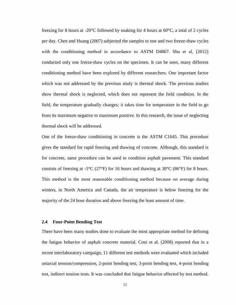
2.4 Four-Point Bending Test
There have been many studies done to evaluate the most appropriate method for defining
the fatigue behavior of asphalt concrete material. Coni et al. (2008) reported that in a
recent interlaboratory campaign, 11 different test methods were evaluated which included
uniaxial tension/compression, 2-point bending test, 3-point bending test, 4-point bending
test, indirect tension tests. It was concluded that fatigue behavior affected by test method.

12
In another study by Tangella et al. (1990), it was concluded that the repeated flexure test
received the highest approval and gave the most representative fatigue behavior amongst
other test methods. From the previously done research and current practice, the most
effective test method is four-point bending test.
The four-point bending test is the most common test used to determine the fatigue
behavior of asphalt concrete. Four-point bending test subjects the middle one-third of the
beam to pure bending, hence, no shear deformation. The standard used for the beam
fatigue is AASHTO T 321 and ASTM D7460. Typically, two loading modes are used:
controlled strain and controlled stress. Controlled strain is used for thinner pavement,
whereas, controlled stress is used for pavement with thicker sections. The number of
cycles at 50% of its initial stiffness can be considered the fatigue life of the asphalt
mixture for that particular tested strain or stress level. Although, previously some
researchers (Pell and Cooper, 1975; Tayebali et al., 1992; Rowe, 1993) have used
constant stress, the common practice is to test with a constant strain mode, which is also
the standard in AASHTO T 321.
2.5 Indirect Tensile Strength Test
Indirect tensile (IDT) strength test is an important test in designing a pavement structure.
With the recent use of Mechanical Empirical Pavement Design Guide (MEPDG)
developed by AASHTO, the tensile strength plays an important parameter in predicting
the low temperature cracking in asphalt pavement.
In 1978, Lottman presented in a NCHRP report the procedure of testing asphalt
cylindrical sample. He proposed the Lottman procedure, in which the specimens are 4
inches in diameter and 2.5 inches in height and the air void content target to be between 4
13
to 8%. The procedure was then finalized as AASHTO T 322 to test indirect tensile
strength of samples.
Another standard, AASHTO T 283, which determines the resistance of compacted
bituminous mixture to moisture damage, is also widely used. This method is used to
determine the change diametral tensile strength from conditioning in the laboratory. This
method is the most appropriate method in testing cylindrical asphalt samples and finding
the tensile strength.
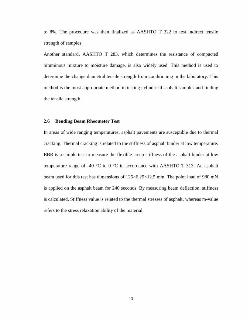
2.6 Bending Beam Rheometer Test
In areas of wide ranging temperatures, asphalt pavements are susceptible due to thermal
cracking. Thermal cracking is related to the stiffness of asphalt binder at low temperature.
BBR is a simple test to measure the flexible creep stiffness of the asphalt binder at low
temperature range of -40 °C to 0 °C in accordance with AASHTO T 313. An asphalt
beam used for this test has dimensions of 125×6.25×12.5 mm. The point load of 980 mN
is applied on the asphalt beam for 240 seconds. By measuring beam deflection, stiffness
is calculated. Stiffness value is related to the thermal stresses of asphalt, whereas m-value
refers to the stress relaxation ability of the material.
14
2.7 Remarks
This chapter has discussed the previous and ongoing research on the freeze-thaw
conditioning of asphalt material. Although, there have been some research done to find
some engineering properties of asphalt after freeze-thaw, no attempt has been done to
study the fatigue life of asphalt pavement over several freeze-thaw cycles using the four-
point bending test. In chapter 3, the research method will be discussed on fatigue life of
asphalt as well as other characteristic tests such as IDT strength test and BBR test.
15
3 CHAPTER 3
SAMPLE PREPARATION AND LABORATORY TESTING
3.1 Experimental Plan
SP-III, commonly used in New Mexico Highways, with PG 70-22 binder is used for this
study. SP-III is mostly used due to its resistance to fatigue cracking and is used in the
intermediate layer of pavement structure.
Hot Mix Asphalt mixture is collected from the construction site for testing purposes.
Samples are collected in accordance with AASHTO T-168 for bituminous mixtures. Bags
of 15kg samples are collected directly from the road site. 15kg is the most efficient
weight for sampling and later for heating the sample for compaction. On average a single
slab for preparing beam samples is 12kg, 3kg extra is taken for material loss while
heating and transporting.
3.2 HMA Mixture Gradation
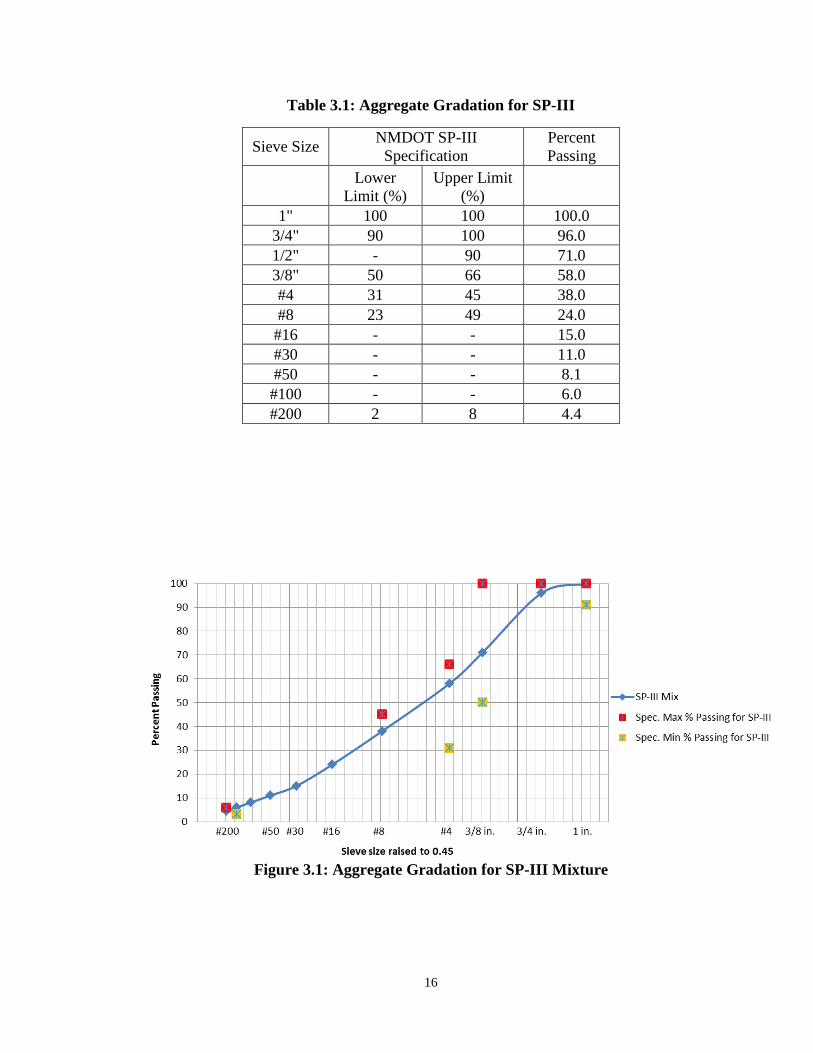
Table 3.1 shows aggregate gradations of SP-III mixture samples. Upper and lower limits
of the mix are also shown in table 3.1. It can be seen that the sample gradation falls
within the NMDOT specification for SP-III mix. Figure 3.1 represents the aggregate
gradation chart for SP-III mixture. The maximum density line for maximum aggregate
sizes of 1 inch is plotted. The mixture plots below the maximum density line, which
represents a coarser mix.
16
Table 3.1: Aggregate Gradation for SP-III
Sieve Size NMDOT SP-III
Specification
Percent
Passing
Lower
Limit (%)
Upper Limit
(%)
1" 100 100 100.0
3/4" 90 100 96.0
1/2" - 90 71.0
3/8" 50 66 58.0
#4 31 45 38.0
#8 23 49 24.0
#16 - - 15.0
#30 - - 11.0
#50 - - 8.1
#100 - - 6.0
#200 2 8 4.4
Figure 3.1: Aggregate Gradation for SP-III Mixture

17
3.3 Sample Preparation
3.3.1 Beam Specimen
According to AASHTO T321, a sample size of 380 mm x 65 mm x 50 mm (15″ x 2.5″ x
2″) must be achieved for the testing of laboratory beam fatigue testing. Samples are
heated and transferred in accordance with AASHTO T312. A target heating temperature
280°F and a target molding temperature of 280°F is achieved (NMDOT Specifications).
The samples are heated for no more than an hour and a half to ensure no additional aging
occurs. The weights of samples are taken using a digital scale to ensure accuracy and are
then transferred to the compactor.
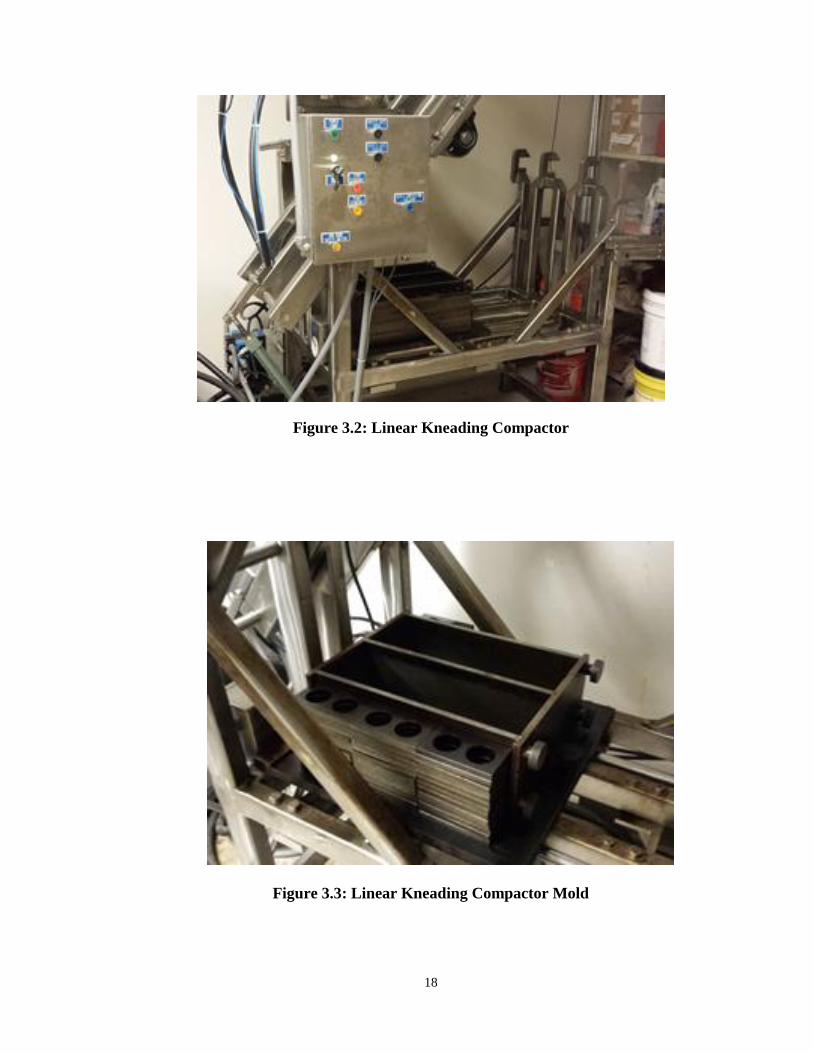
Linear kneading compactor shown in figures 3.2 and 3.3, is constructed of stainless steel
and 1045 steel and powered by 208/230 Volt 3-Phase, to create beam slabs. The
compactor is operated by a hydraulic unit. The compactor has the capability of creating a
larger than the standard samples, at which point, the slab is cut from all directions to
achieve a final smooth beam of 380 mm x 65 mm x 50 mm (15″ x 2.5″ x 2″).
18
Figure 3.2: Linear Kneading Compactor
Figure 3.3: Linear Kneading Compactor Mold
19
3.3.2 Cylindrical Specimen
Cylindrical sample are prepared using a pine gyrator compactor. The compactor is
equipped to set the maximum number of gyration of the mold or a minimum height
requirement for the sample inside the mold. The gyratory compactor produces sample
sizes of 8 inches high and 6 inches in diameter. As with the beam samples, the target
heating temperature 280°F and a target molding temperature of 280°F is achieved
(NMDOT Specifications). The samples are heated for no more than an hour and a half,
until workable. The weights of samples are taken using a digital scale and are then
transferred to the compactor. Figure 3.4 shows the gyratory compactor and figure 3.5
shows a molded sample with a height of 8 inches and diameter of 6 inches.

20
Figure 3.4: Pine Gyratory Compactor
Figure 3.5: Molded Sample with 8 inches Height and 6 inches Diameter

21
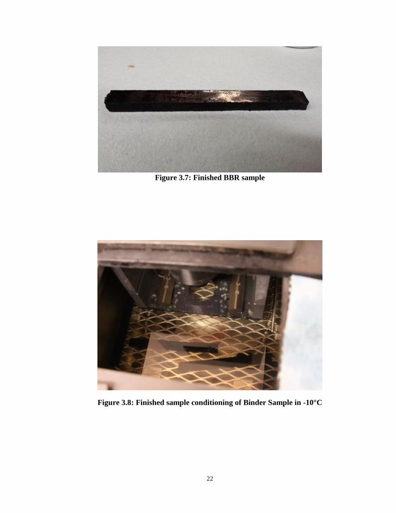
3.3.3 BBR Specimen
BBR samples are prepared in accordance to AASHTO T 313. Samples sizes are 6.25 mm
x 12.5mm x 100mm. The binder is heated at 300°C and heated long enough until it is in
workable fluid state. During the heating process, samples must be covered and also
stirred to ensure equal aging and homogeneity. This procedure will remove air bubbles to
avoid any voids in the specimen. In a mold, the binder is poured. The sample is trimmed,
seen in figure 3.6, and taken out of the mold after 45 to 60 minutes of cooling. The
finished sample, at room temperature, can be seen in figure 3.7. The binder beam samples
must be in a bath at the desired testing temperature for 60 minutes for conditioning, seen
in figure 3.8.
Figure 3.6: Trimming of Room Temperature Binder Sample
22
Figure 3.7: Finished BBR sample
Figure 3.8: Finished sample conditioning of Binder Sample in -10°C
23
3.4 Sample Cutting
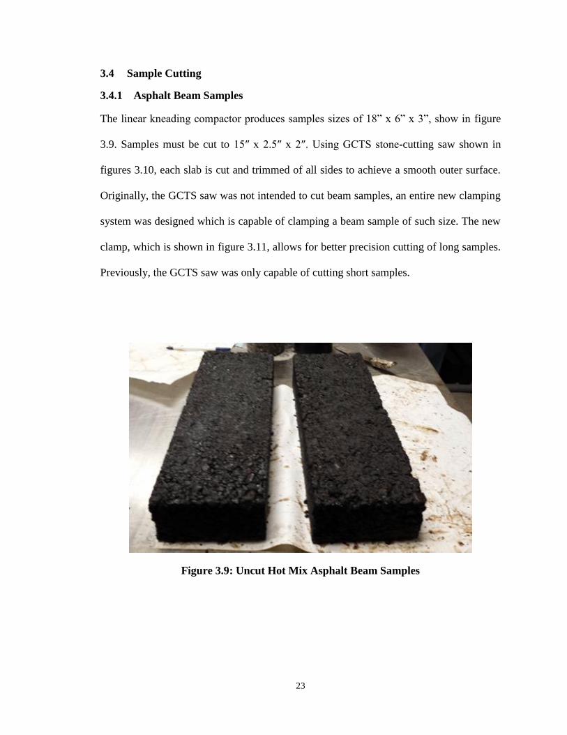
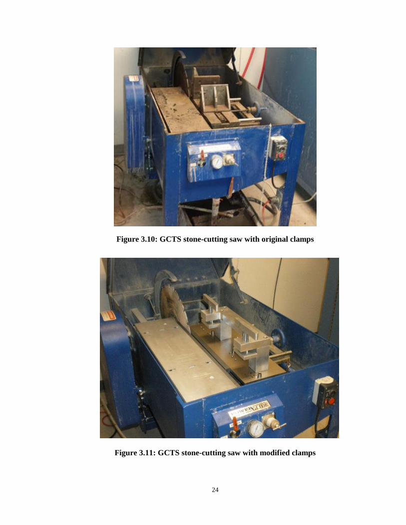
3.4.1 Asphalt Beam Samples
The linear kneading compactor produces samples sizes of 18” x 6” x 3”, show in figure
3.9. Samples must be cut to 15″ x 2.5″ x 2″. Using GCTS stone-cutting saw shown in
figures 3.10, each slab is cut and trimmed of all sides to achieve a smooth outer surface.
Originally, the GCTS saw was not intended to cut beam samples, an entire new clamping
system was designed which is capable of clamping a beam sample of such size. The new
clamp, which is shown in figure 3.11, allows for better precision cutting of long samples.
Previously, the GCTS saw was only capable of cutting short samples.
Figure 3.9: Uncut Hot Mix Asphalt Beam Samples
24
Figure 3.10: GCTS stone-cutting saw with original clamps
Figure 3.11: GCTS stone-cutting saw with modified clamps

25
3.4.2 Asphalt Cylinder Samples
The gyratory compactor produces sample sizes of 8 inches high and 6 inches in diameter.
The standard for IDT, AASHTO T 283, calls for samples sizes to be 4 inches (100mm) in
diameter and 2.5 ±.1 inches (63.5 ± 2.5 mm) in thickness. The compacted sample must
first be cored to a 4 in diameter thickness using GCTS Pressure Controlled Core Drill
seen in figure 3.12. Once, the correct diameter is achieved, the sample is then cut using
GCTS stone-cutting saw.
Figure 3.12: GCTS Pressure Controlled Core Drill

26
3.5 Specimen Volumetric Analysis
Maximum Specific Gravity (Gmm) is done in accordance with ASTM D6857. The
CoreLok system, which is a system for sealing asphalt samples so that the sample
densities are measured, is used as an alternative to the conventional “Rice Test” for the
determination of maximum specific gravity of loose asphalt mixtures. The Corelok
automatically seals the samples in a puncture resistant polymer bags. The samples are
dried previously and then placed inside the vacuum bags. The bags are sealed with the
CoreLok vacuum chamber. Then, the bags are cut open under water and the weight is
taken while the sample is still submerged in water. Average Gmm for the mix used is
2.516. The calculations for determining Gmm are as follows:
(3.1)
Where,
A = weight of dry sample in air, (grams)
B = weight of bag, (grams)
C = weight of sample open in water, (grams)
Bulk specific gravity (Gmb) is performed on asphalt beam samples according to
AASHTO T269. The weight of the sample is taken under three different conditions: dry,
saturated surface dry, and submerged in water. Gmb can be calculated using the
following:
(3.2)
Where,
Gmb = Bulk specific gravity
A = Mass of sample in Air

27
B = Mass of sample saturated surface dry
C = Mass of sample submerged in water
The target air voids in the compacted mixture for this study is between 5 and 6%. The air
voids can be calculated using following:
(3.3)
Where,
VTM = Air voids in the compacted mixture
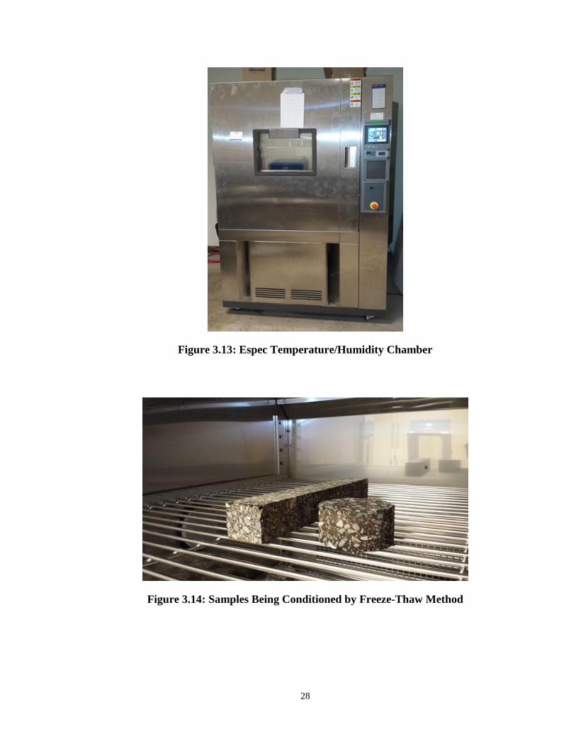
3.6 Sample Conditioning
Samples are conditioned according to ASTM C1645 which calls for freezing at -5°C for
16 hours and +30°C for 8 hours. -5°C and +30°C are chosen as target temperatures
because they represent field conditions. In New Mexico, air temperatures reach on
average of -5°C during winter and +30°C is a representative temperature to thaw the
HMA. Moreover, by having greater freezing time, it simulates more damage in the HMA
due to ice forming in the HMA and expanding. After completing these two stages, it is
considered one cycle. As well as conditioning the samples to freezing and thawing,
humidity is also included. At -5°C, at humidity level of 15% is induced, which is the
average humidity in December in New Mexico. At +30°C, a humidity level of 40% is
induced. The freeze-thaw and humidity conditioning is done with an Espec
temperature/humidity chamber, shown in figure 3.13 and 3.14. The Espec chamber is an
automatic temperature/humidity controller. This reduces the risk of any human error.
28
Figure 3.13: Espec Temperature/Humidity Chamber
Figure 3.14: Samples Being Conditioned by Freeze-Thaw Method
29
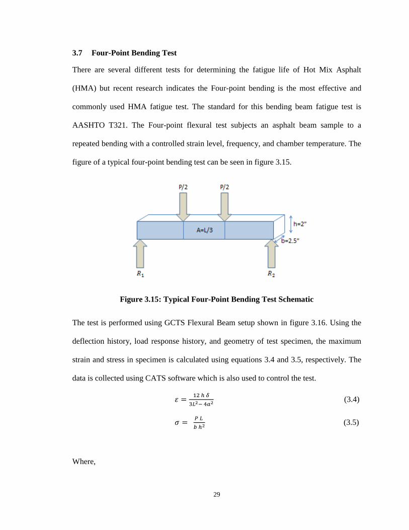
3.7 Four-Point Bending Test
There are several different tests for determining the fatigue life of Hot Mix Asphalt
(HMA) but recent research indicates the Four-point bending is the most effective and
commonly used HMA fatigue test. The standard for this bending beam fatigue test is
AASHTO T321. The Four-point flexural test subjects an asphalt beam sample to a
repeated bending with a controlled strain level, frequency, and chamber temperature. The
figure of a typical four-point bending test can be seen in figure 3.15.
Figure 3.15: Typical Four-Point Bending Test Schematic
The test is performed using GCTS Flexural Beam setup shown in figure 3.16. Using the
deflection history, load response history, and geometry of test specimen, the maximum
strain and stress in specimen is calculated using equations 3.4 and 3.5, respectively. The
data is collected using CATS software which is also used to control the test.
(3.4)
(3.5)
Where,
30
ε = maximum strain
ζ = maximum stress
P = load applied by actuator at time t
b = average specimen width
h = average specimen height
δ = deflection at center of beam at time t
a = distance between inside clamps
L = distance between outside clamps.
Sample flexural stiffness is then calculated using ζ and ε data recorded from each cycle.
(3.6)
Where,
E = flexural modulus
Then, number of cycles at 50% reduction in stiffness is recorded as failure of beam
according to AASHTO T 321. Testing is conducted in constant strain mode. Each beam
sample is sinusoidally loaded at a frequency of 10 Hz and at a constant temperature of
20±0.5°C. The beam fatigue test setup with the LVDT attached can be seen in figure
3.17.

31
Figure 3.16: GCTS Flexural Beam Setup
Figure 3.17: Beam Fatigue Test Setup with the LVDT Attached

32
3.8 Indirect Tensile Strength Test
Indirect Tensile (IDT) Strength Test was done according to AASHTO T 283. The sample
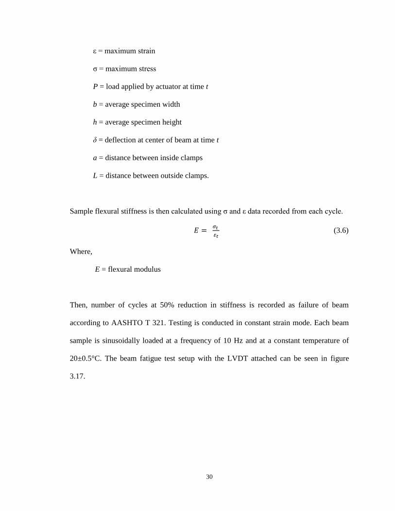
size of 4 inches (100mm) in diameter and 2.5 ±.1 inches (63.5 ± 2.5 mm) in thickness is
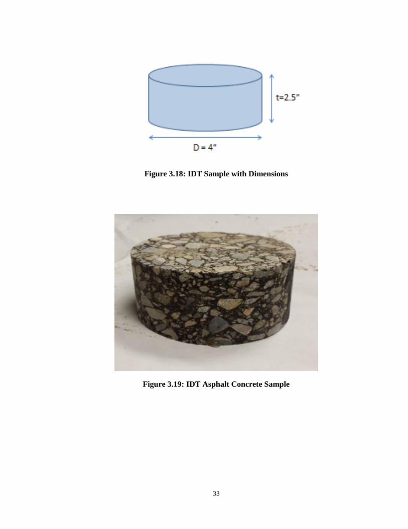
maintained. Figures 3.18 and 3.19 display a typical IDT sample with dimensions. The
load was applied to the specimen at constant rate of 2 inches/minute (50 mm/minute). A
typical IDT test set up with a specimen is shown in figure 3.20. The sample tensile
strength is calculated using:
(3.7)
Where,
= tensile strength, psi
P = maximum load, lbf
t = specimen thickness, inches
D = specimen diameter
The effect of freeze-thaw is further analyzed as the ratio of the original strength that is
retained after the freeze-thaw conditioning. The tensile strength ratio is calculated as:
(3.8)
Where,
= average tensile strength of control, kPa
= average tensile strength of the conditioned, kPa
33
Figure 3.18: IDT Sample with Dimensions
Figure 3.19: IDT Asphalt Concrete Sample

34
Figure 3.20: IDT Test Setup with a Specimen
35
3.9 Bending Beam Rheometer Test
The Bending Beam Rheometer (BBR) test is done according to AASHTO T 313. BBR
test is used to study the stiffness of binder at low temperatures. Samples are tested at -
10°C; Creep stiffness and m-value, which is the slope of the master stiffness curve, is
determined. The standard calls for a constant creep load of 980 mN on the asphalt binder
beam for 240 seconds and the measured values for stiffness and m-values at 60 seconds
are used. The stiffness of the asphalt binder beam is calculated using:
(3.9)
Where,
S(t) = time-dependent flexural creep stiffness, MPa
P = constant load, N
L = span length, mm
b = width of beam, mm
h = thickness of beam, mm
δ(t) = deflection of beam, mm
δ(t) and S(t) indicate that the deflection and stiffness are functions of time.
The time displacement data is extracted for further analysis and stiffness and m-value
calculation.
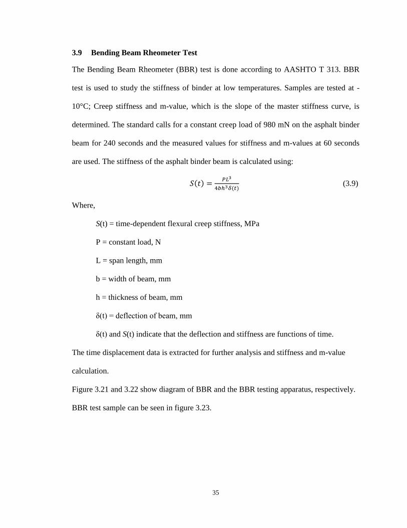
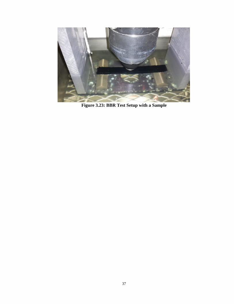
Figure 3.21 and 3.22 show diagram of BBR and the BBR testing apparatus, respectively.
BBR test sample can be seen in figure 3.23.

36
Figure 3.21: BBR Sample with Dimensions
Figure 3.22: BBR Testing Apparatus
37
Figure 3.23: BBR Test Setup with a Sample

38
4 CHAPTER 4
EFFECT OF FREEZE-THAW ON BEAM FATIGUE
PARAMETERS
4.1 Introduction
In this section, laboratory test results of flexure beam test are analyzed. The objective of
this study is to characterize the evolution of freeze-thaw damage on the decrease of
modulus and fatigue life of AC. All samples are conditioned similarly with different
freeze-thaw cycles for each set of samples. Table 4.1 presents the test matrix for the four-
point bending test. One Hot Mix Asphalt (HMA) mixture was used for this study with a
PG 70-22 binder. The material is collected from District 2, New Mexico. The applied
strain amplitude is fixed at 400µε with the number of freeze-thaw varying from 0 to 20
cycles. The target air voids content in the samples are 5.5 ± .5%.
Table 4.1: Test Matrix for Four-Point Bending Test
HMA mix
type
PG
binder
Applied
Strain
Air Void
Content
Freeze-Thaw
Cycles
SP-III 70-22 400µε 5.5 ± .5%
0
5
10
15
20

39
4.2 Fatigue Test
Asphalt beam flexure tests are conducted using a four-point bending schematic. The tests
are performed at 400µε amplitude, frequency of 10Hz, and control temperature of 20 ± .5
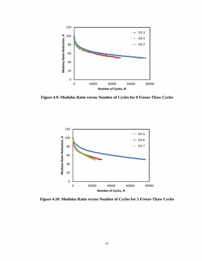
°C. The tests are performed to determine the flexure modulus reduction after each set of
freeze-thaw conditioning. Table 4.1 presents the test results for the laboratory flexure test
along with the sample ID, freeze-thaw cycle number, air void ratio, initial modulus, and
number of cycles to failure.
4.2.1 Results and Discussion on Beam Fatigue Test
In the fatigue test, using the displacement and load history, stiffness was recorded every
cycle. In figure 4.1, the initial modulus is plotted against different cycles of freeze-thaw.
For each column, 3 different samples are tested and the average modulus obtained is
plotted. The average initial modulus of the control is 1,055,093 psi. For 5, 10, 15, and 20
freeze-thaw cycles, the obtained modulus are 999,046 psi, 992,816 psi, 959,765 psi,
878,328 psi, respectively. A trend can be seen, as the number of freeze-thaw cycles
increases, the average initial modulus decreases. This finding is in correlation with the
fact that freeze-thaw conditioning induces damage into asphalt pavement and the
repetitive freeze-thaw promotes increasing damage. The damage causes the initial
modulus of the pavement to decrease. Although, the case may be true for the average,
different results were found for individual cases. For higher freeze-thaw cycles, it was
seen that some samples gave a higher initial modulus than the previous samples. This
type of behavior is expected with the conditioning method because freeze-thaw ages the
binder. The aging of binder makes the sample stiffer. While this may be true for general

40
cases, some samples showed a decrease in modulus which suggests the freeze-thaw
damage has effect on the adhesion between the binder and aggregate. The result of that is
a less stiff material.
Figure 4.1: Stiffness versus Different Numbers of Freeze-Thaw Cycles Curve
Figure 4.2 compares the fatigue life for different freeze-thaw cycles. It was recorded that
the average fatigue life for control (0 freeze-thaw cycles) was 66,601 cycles. For the 5
day freeze-thaw cycle, the average fatigue life decreased to 42,728 cycles. It was seen
that the average fatigue life stayed the same, 42,534 cycles to failure. It is worth noting
that the most change in fatigue occurred between the 0 and 5 freeze-thaw cycles then the
fatigue tends to stabilized. For the 15 freeze-thaw cycles, the fatigue life decreased to
30,868 cycles. 20 freeze-thaw cycles, resulted in higher fatigue life than 15 freeze-thaw
cycles. This is due to the behavior of some samples producing higher fatigue lives than of
15 freeze-thaw cycles. It can be seen in table 4.1 that the initial modulus of 20 freeze-
thaw cycles are less than 15, yet the produced a greater fatigue life. It is worth noting that
0
200
400
600
800
1000
1200
0 5 10 15 20
Mo
du
lus,
ksi
Freeze-Thaw Cycles
0
5
10
15
20

41
higher initial modulus sometimes does not produce a greater life. As samples age, they
become stiffer i.e. more brittle. With the repetitive loading mode, higher initial modulus
does not necessarily produce a greater fatigue life, as they will crack sooner.
Figure 4.2: Comparison of Number of Cycles to Failure with Different Freeze-Thaw
Cycles
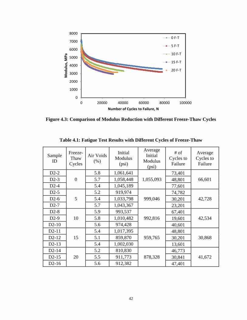
Moreover, modulus-number of cycles to failure is plotted for different freeze-thaw cases,
shown in figure 4.3. The figure represents a sample from every batch of freeze-thaw.
Two things can be noted here, as number of freeze-thaw increases the graph becomes
shorter horizontally, i.e. fails quicker. Also, as the number of freeze-thaw cycles
increases, the lines on the graph drops lower which indicates a drop in modulus. The
result is very acceptable because as predicted, the freeze-thaw conditioning should cause
damage to asphalt samples, which should decrease the modulus, as well as have an effect
on the fatigue life of asphalt pavement.
0
10000
20000
30000
40000
50000
60000
70000
80000
90000
0 5 10 15 20
Ave
rage
Cyc
les
to f
ailu
re, N
Average of Different Freeze-Thaw Batches
0
5
10
15
20
42
Figure 4.3: Comparison of Modulus Reduction with Different Freeze-Thaw Cycles
Table 4.1: Fatigue Test Results with Different Cycles of Freeze-Thaw
Sample
ID
Freeze-
Thaw
Cycles
Air Voids
(%)
Initial
Modulus
(psi)
Average
Initial
Modulus
(psi)
# of
Cycles to
Failure
Average
Cycles to
Failure
D2-2
0
5.8 1,061,641
1,055,093
73,401
66,601 D2-3 5.7 1,058,448 48,801
D2-4 5.4 1,045,189 77,601
D2-5
5
5.2 919,974
999,046
74,782
42,728 D2-6 5.4 1,033,798 30,201
D2-7 5.7 1,043,367 23,201
D2-8
10
5.9 993,537
992,816
67,401
42,534 D2-9 5.8 1,010,482 19,601
D2-10 5.6 974,428 40,601
D2-11
15
5.4 1,017,395
959,765
48,801
30,868 D2-12 5.1 859,870 30,201
D2-13 5.4 1,002,030 13,601
D2-14
20
5.2 810,830
878,328
46,773
41,672 D2-15 5.5 911,773 30,841
D2-16 5.6 912,382 47,401
0
1000
2000
3000
4000
5000
6000
7000
8000
0 20000 40000 60000 80000 100000
Mo
du
lus,
MP
a
Number of Cycles to Failure, N
0 F-T
5 F-T
10 F-T
15 F-T
20 F-T
43
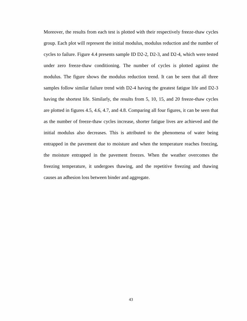
Moreover, the results from each test is plotted with their respectively freeze-thaw cycles
group. Each plot will represent the initial modulus, modulus reduction and the number of
cycles to failure. Figure 4.4 presents sample ID D2-2, D2-3, and D2-4, which were tested
under zero freeze-thaw conditioning. The number of cycles is plotted against the
modulus. The figure shows the modulus reduction trend. It can be seen that all three
samples follow similar failure trend with D2-4 having the greatest fatigue life and D2-3
having the shortest life. Similarly, the results from 5, 10, 15, and 20 freeze-thaw cycles
are plotted in figures 4.5, 4.6, 4.7, and 4.8. Comparing all four figures, it can be seen that
as the number of freeze-thaw cycles increase, shorter fatigue lives are achieved and the
initial modulus also decreases. This is attributed to the phenomena of water being
entrapped in the pavement due to moisture and when the temperature reaches freezing,
the moisture entrapped in the pavement freezes. When the weather overcomes the
freezing temperature, it undergoes thawing, and the repetitive freezing and thawing
causes an adhesion loss between binder and aggregate.

44
Figure 4.4: Modulus versus Number of Cycles for 0 Freeze-Thaw Cycles
Figure 4.5: Modulus versus Number of Cycles for 5 Freeze-Thaw Cycles
0
1000
2000
3000
4000
5000
6000
7000
8000
0 20000 40000 60000 80000
Mo
du
lus,
MP
a
Number of Cycles, N
D2-3
D2-4
D2-2
0
1000
2000
3000
4000
5000
6000
7000
8000
0 20000 40000 60000 80000
Mo
du
lus,
MP
a
Number of Cycles, N
D2-5
D2-6
D2-7

45
Figure 4.6: Modulus versus Number of Cycles for 10 Freeze-Thaw Cycles
Figure 4.7: Modulus versus Number of Cycles for 15 Freeze-Thaw Cycles
0
1000
2000
3000
4000
5000
6000
7000
8000
0 20000 40000 60000 80000
Mo
du
lus,
MP
a
Number of Cycles, N
D2-8
D2-9
D2-10
0
1000
2000
3000
4000
5000
6000
7000
8000
0 20000 40000 60000 80000
Mo
du
lus,
MP
a
Number of Cycles, N
D2-11
D2-13
D2-12
46
Figure 4.8: Modulus versus Number of Cycles for 20 Freeze-Thaw Cycles
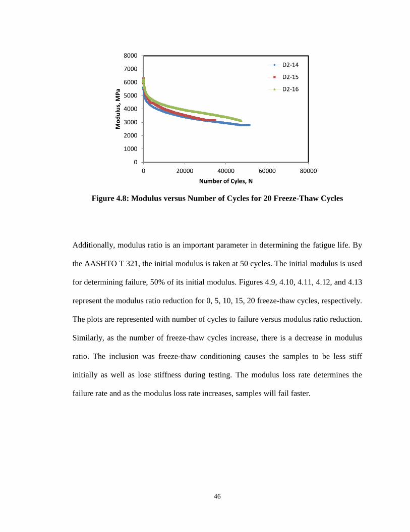
Additionally, modulus ratio is an important parameter in determining the fatigue life. By
the AASHTO T 321, the initial modulus is taken at 50 cycles. The initial modulus is used
for determining failure, 50% of its initial modulus. Figures 4.9, 4.10, 4.11, 4.12, and 4.13
represent the modulus ratio reduction for 0, 5, 10, 15, 20 freeze-thaw cycles, respectively.
The plots are represented with number of cycles to failure versus modulus ratio reduction.
Similarly, as the number of freeze-thaw cycles increase, there is a decrease in modulus
ratio. The inclusion was freeze-thaw conditioning causes the samples to be less stiff
initially as well as lose stiffness during testing. The modulus loss rate determines the
failure rate and as the modulus loss rate increases, samples will fail faster.
0
1000
2000
3000
4000
5000
6000
7000
8000
0 20000 40000 60000 80000
Mo
du
lus,
MP
a
Number of Cyles, N
D2-14
D2-15
D2-16
47
Figure 4.9: Modulus Ratio versus Number of Cycles for 0 Freeze-Thaw Cycles
Figure 4.10: Modulus Ratio versus Number of Cycles for 5 Freeze-Thaw Cycles
0
20
40
60
80
100
120
0 20000 40000 60000 80000
Mo
du
lus
Rat
io R
ed
uct
ion
, %
Number of Cycles, N
D2-3
D2-4
D2-2
0
20
40
60
80
100
120
0 20000 40000 60000 80000
Mo
du
lus
Rat
io R
ed
uct
ion
, %
Number of Cycles, N
D2-5
D2-6
D2-7

48
Figure 4.11: Modulus Ratio versus Number of Cycles for 10 Freeze-Thaw Cycles
Figure 4.12: Modulus Ratio versus Number of Cycles for 15 Freeze-Thaw Cycles
0
20
40
60
80
100
120
0 20000 40000 60000 80000
Mo
du
lus
Rat
io R
ed
uct
ion
, %
Number of Cycles, N
D2-8
D2-9
D2-10
0
20
40
60
80
100
120
0 20000 40000 60000
Mo
du
lus
Rat
io R
ed
uct
ion
, %
Number of Cyles, N
D2-11
D2-12
D2-13
49
Figure 4.13: Modulus Ratio versus Number of Cycles for 20 Freeze-Thaw Cycles
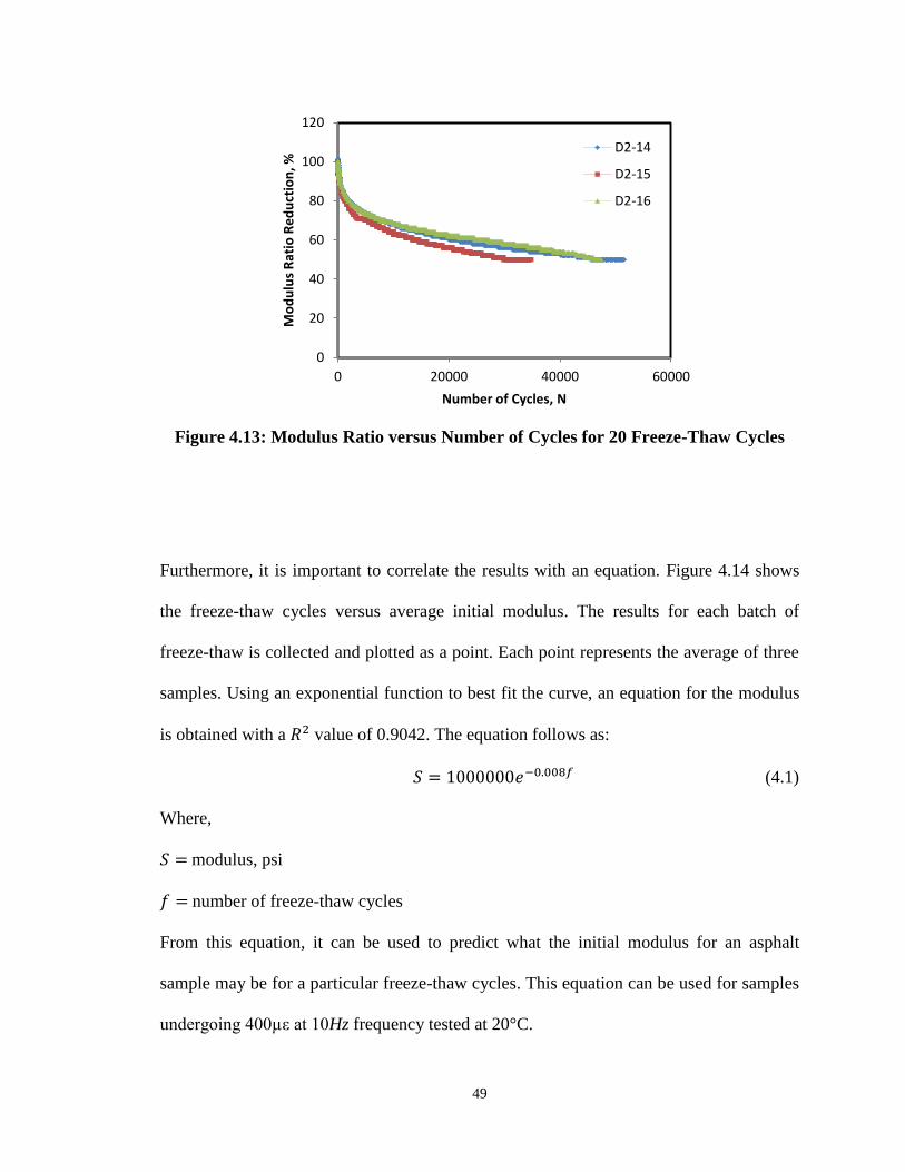
Furthermore, it is important to correlate the results with an equation. Figure 4.14 shows
the freeze-thaw cycles versus average initial modulus. The results for each batch of
freeze-thaw is collected and plotted as a point. Each point represents the average of three
samples. Using an exponential function to best fit the curve, an equation for the modulus
is obtained with a value of 0.9042. The equation follows as:
(4.1)
Where,
modulus, psi
number of freeze-thaw cycles
From this equation, it can be used to predict what the initial modulus for an asphalt
sample may be for a particular freeze-thaw cycles. This equation can be used for samples
undergoing 400µε at 10Hz frequency tested at 20°C.
0
20
40
60
80
100
120
0 20000 40000 60000
Mo
du
lus
Rat
io R
ed
uct
ion
, %
Number of Cycles, N
D2-14
D2-15
D2-16

50
Figure 4.14: Correlation of Initial Modulus with Increasing Number of F-T Cycles
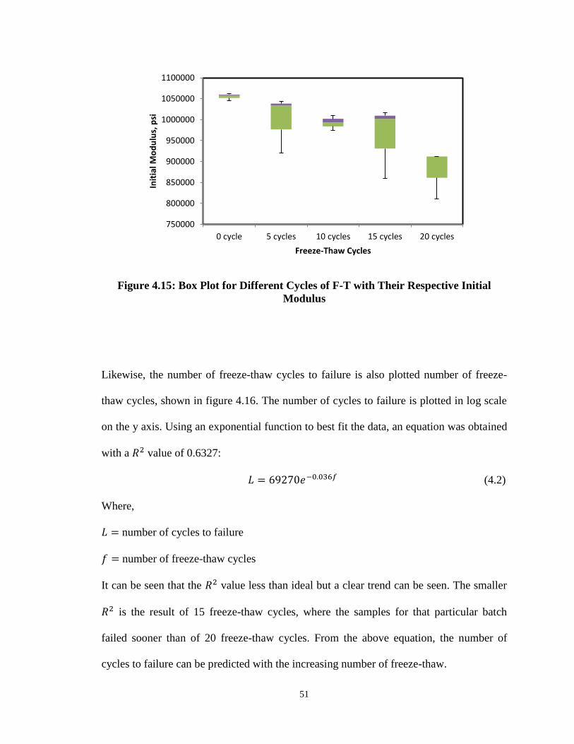
Furthermore, in figure 4.15, the box plot for each class of freeze-thaw shows median, ¼
quartile, ¾ quartile and variation range of the data. It can be seen that the modulus
decreases with increase in freeze-thaw cycle. It can be said that freeze-thaw conditioning
is decreasing the modulus of the material and increasing the damage in the sample.
Modulus data for each class of freeze-thaw is further analyzed for ANOVA analysis.
Data analysis is done in statistical software R. The analysis is done with the assumption
that the normality assumption holds true. From ANOVA analysis, for different freeze-
thaw cycles, a p-value of 0.06681 is obtained, which is less than 0.1 (90% confidence
interval). Therefore, it can be said that there is a statistical difference between the mean
of each group. To further analyze which mean is different from the control samples, t-test
is used. From t-test, it is seen a statistical difference can be seen after 10 cycles of freeze-
thaw.
y = 1E+06e-0.008x
R² = 0.9042
0
200000
400000
600000
800000
1000000
1200000
0 5 10 15 20 25
Init
ial M
od
ulu
s, p
si
Freeze-Thaw Cycles
Avg InitialStiffness, psi
Expon. (AvgInitial Stiffness,psi)
51
Figure 4.15: Box Plot for Different Cycles of F-T with Their Respective Initial
Modulus
Likewise, the number of freeze-thaw cycles to failure is also plotted number of freeze-
thaw cycles, shown in figure 4.16. The number of cycles to failure is plotted in log scale
on the y axis. Using an exponential function to best fit the data, an equation was obtained
with a value of 0.6327:
(4.2)
Where,
number of cycles to failure
number of freeze-thaw cycles
It can be seen that the value less than ideal but a clear trend can be seen. The smaller
is the result of 15 freeze-thaw cycles, where the samples for that particular batch
failed sooner than of 20 freeze-thaw cycles. From the above equation, the number of
cycles to failure can be predicted with the increasing number of freeze-thaw.
750000
800000
850000
900000
950000
1000000
1050000
1100000
0 cycle 5 cycles 10 cycles 15 cycles 20 cycles
Init
ial M
od
ulu
s, p
si
Freeze-Thaw Cycles

52
Figure 4.16: Correlation of Number of Cycles to Failure to F-T Cycles
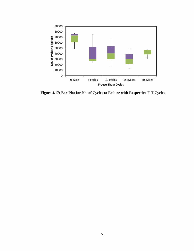
In addition, in figure 4.17, the box plot for each class of freeze-thaw with respect to
number of cycles to failure is shown. The figure shows median, ¼ quartile, ¾ quartile and
variation range of the data. It can be seen that there is a decreasing trend in the number of
cycles to failure with increasing freeze-thaw. From the box plot, it can be seen a wider
range for 5, 10, and 10 freeze-thaw cycles, but the overall trend shows a decrease in
fatigue life. From ANOVA analysis, for different freeze-thaw cycles, a p-value of
0.08399 is obtained, which is less than 0.1. The p-value implies there is detectable
difference between the mean of each group. Therefore, the mean there is evidence that
the mean of each group is different from each other. To further analyze which mean is
different from the control sample, t-test is performed. From t-test, it is shown the mean of
the 15 days is different than of 0 days.
y = 69270e-0.036x
R² = 0.6327
100
1000
10000
100000
1000000
0 5 10 15 20 25
Nu
mb
e o
f C
ycl
es t
o F
ail
ure
in
lo
g, N
Freeze-Thaw Cycles
Average Cycles toFailure
Expon. (AverageCycles to Failure)
53
Figure 4.17: Box Plot for No. of Cycles to Failure with Respective F-T Cycles
0
10000
20000
30000
40000
50000
60000
70000
80000
90000
0 cycle 5 cycles 10 cycles 15 cycles 20 cycles
No
. of
cycl
es
to F
ailu
re
Freeze-Thaw Cycles
54
5 CHAPTER 5
EFFECTS OF FREEZE-THAW ON INDIRECT TENSILE
STREGNTH AND BENDING BEAM RHEOMETER
STIFFNESS
5.1 Introduction
In this section, laboratory test results of indirect tensile strength test and bending beam
rheometer test are analyzed. The objective of this study is to characterize the evolution of
freeze-thaw damage on the decrease of stiffness and strength of AC. All samples are
conditioned similarly with different freeze-thaw cycles for each set of samples.
Table 5.1 presents the test matrix for the IDT test. The same mix, collected from the field
in District 2 is used for this study. The air voids content is also maintained at 5.5 ± .5% to
maintain uniformity and represent similar gradation. Similarly, the number of freeze-thaw
varies from 0 to 20 cycles.
Table 5.2 represents the test matrix for the bending beam rheometer test. The binder
grade used for this part of the study is 70-22, the same binder grade used for the HMA.
The binder is conditioned under the same freeze-thaw scheme with the cycles varying
from 0 to 20.

55
Table 5.1: Test Matrix for IDT Test
HMA mix
type
PG
binder
Air Void
Content
Freeze-Thaw
Cycles
SP-III 70-22 5.5 ± .5%
0
5
10
15
20
Table 5.2: Test Matrix for Bending Beam Rheometer Test
PG
binder
Freeze-Thaw
Cycles
70-22
0
5
10
15
20
56
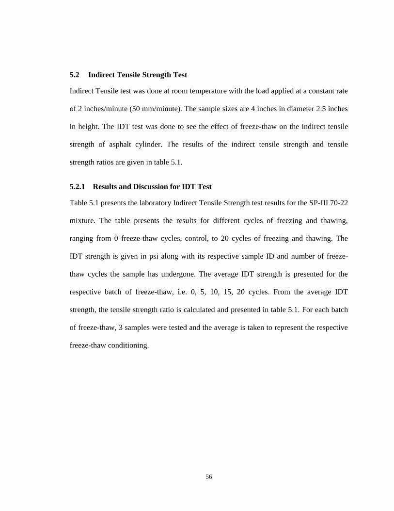
5.2 Indirect Tensile Strength Test
Indirect Tensile test was done at room temperature with the load applied at a constant rate
of 2 inches/minute (50 mm/minute). The sample sizes are 4 inches in diameter 2.5 inches
in height. The IDT test was done to see the effect of freeze-thaw on the indirect tensile
strength of asphalt cylinder. The results of the indirect tensile strength and tensile
strength ratios are given in table 5.1.
5.2.1 Results and Discussion for IDT Test
Table 5.1 presents the laboratory Indirect Tensile Strength test results for the SP-III 70-22
mixture. The table presents the results for different cycles of freezing and thawing,
ranging from 0 freeze-thaw cycles, control, to 20 cycles of freezing and thawing. The
IDT strength is given in psi along with its respective sample ID and number of freeze-
thaw cycles the sample has undergone. The average IDT strength is presented for the
respective batch of freeze-thaw, i.e. 0, 5, 10, 15, 20 cycles. From the average IDT
strength, the tensile strength ratio is calculated and presented in table 5.1. For each batch
of freeze-thaw, 3 samples were tested and the average is taken to represent the respective
freeze-thaw conditioning.
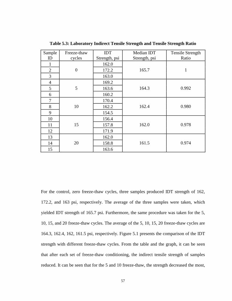
57
Table 5.3: Laboratory Indirect Tensile Strength and Tensile Strength Ratio
Sample
ID
Freeze-thaw
cycles
IDT
Strength, psi
Median IDT
Strength, psi
Tensile Strength
Ratio
1
0
162.0
165.7 1 2 172.2
3 163.0
4
5
169.2
164.3 0.992 5 163.6
6 160.2
7
10
170.4
162.4 0.980 8 162.2
9 154.5
10
15
156.4
162.0 0.978 11 157.8
12 171.9
13
20
162.0
161.5 0.974 14 158.8
15 163.6
For the control, zero freeze-thaw cycles, three samples produced IDT strength of 162,
172.2, and 163 psi, respectively. The average of the three samples were taken, which
yielded IDT strength of 165.7 psi. Furthermore, the same procedure was taken for the 5,
10, 15, and 20 freeze-thaw cycles. The average of the 5, 10, 15, 20 freeze-thaw cycles are
164.3, 162.4, 162, 161.5 psi, respectively. Figure 5.1 presents the comparison of the IDT
strength with different freeze-thaw cycles. From the table and the graph, it can be seen
that after each set of freeze-thaw conditioning, the indirect tensile strength of samples
reduced. It can be seen that for the 5 and 10 freeze-thaw, the strength decreased the most,
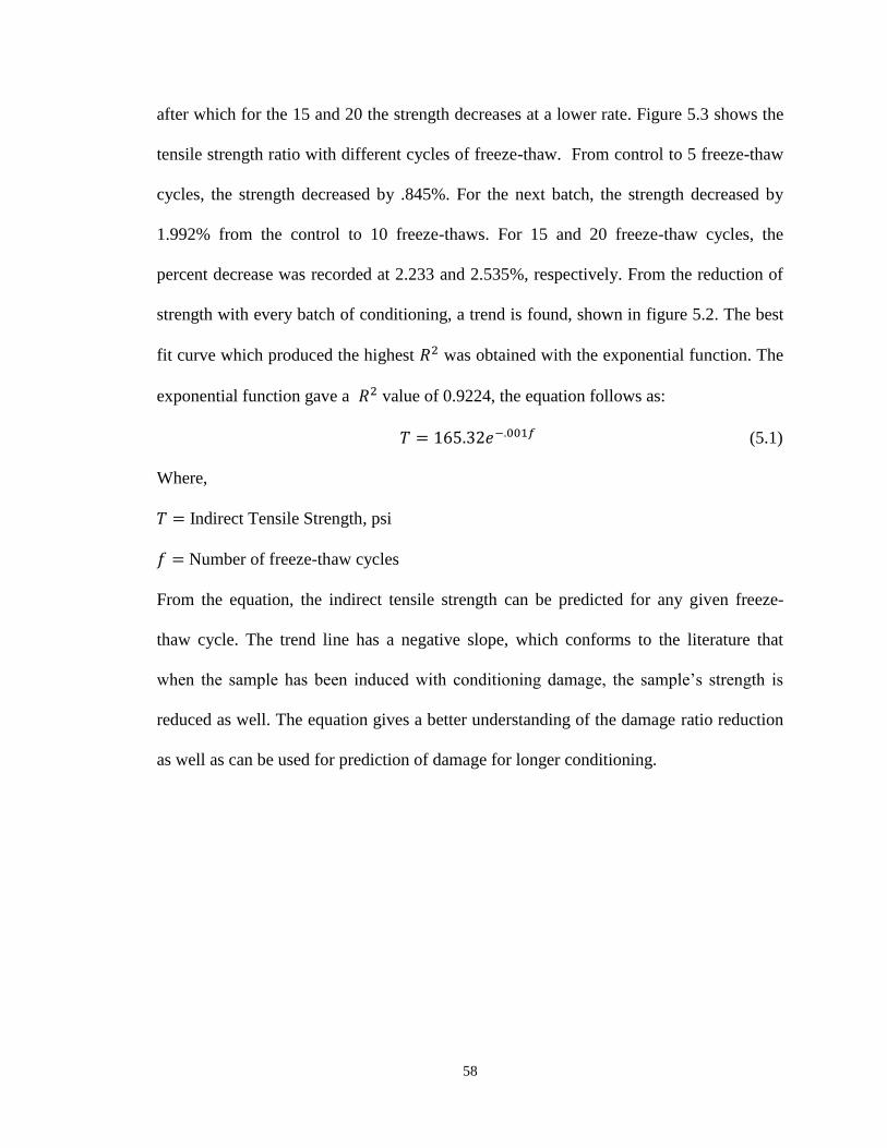
58
after which for the 15 and 20 the strength decreases at a lower rate. Figure 5.3 shows the
tensile strength ratio with different cycles of freeze-thaw. From control to 5 freeze-thaw
cycles, the strength decreased by .845%. For the next batch, the strength decreased by
1.992% from the control to 10 freeze-thaws. For 15 and 20 freeze-thaw cycles, the
percent decrease was recorded at 2.233 and 2.535%, respectively. From the reduction of
strength with every batch of conditioning, a trend is found, shown in figure 5.2. The best
fit curve which produced the highest was obtained with the exponential function. The
exponential function gave a value of 0.9224, the equation follows as:
(5.1)
Where,
Indirect Tensile Strength, psi
Number of freeze-thaw cycles
From the equation, the indirect tensile strength can be predicted for any given freeze-
thaw cycle. The trend line has a negative slope, which conforms to the literature that
when the sample has been induced with conditioning damage, the sample’s strength is
reduced as well. The equation gives a better understanding of the damage ratio reduction
as well as can be used for prediction of damage for longer conditioning.
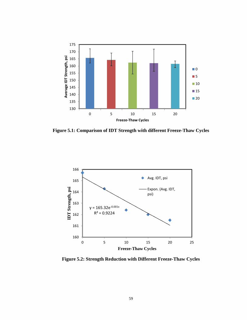
59
Figure 5.1: Comparison of IDT Strength with different Freeze-Thaw Cycles
Figure 5.2: Strength Reduction with Different Freeze-Thaw Cycles
130
135
140
145
150
155
160
165
170
175
0 5 10 15 20
Ave
rage
ID
T St
ren
gth
, psi
Freeze-Thaw Cycles
0
5
10
15
20
y = 165.32e-0.001x R² = 0.9224
160
161
162
163
164
165
166
0 5 10 15 20 25
IDT
Str
ength
, p
si
Freeze-Thaw Cycles
Avg. IDT, psi
Expon. (Avg. IDT,psi)
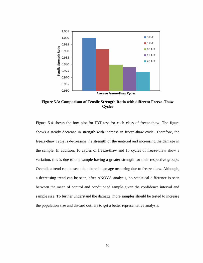
60
Figure 5.3: Comparison of Tensile Strength Ratio with different Freeze-Thaw
Cycles
Figure 5.4 shows the box plot for IDT test for each class of freeze-thaw. The figure
shows a steady decrease in strength with increase in freeze-thaw cycle. Therefore, the
freeze-thaw cycle is decreasing the strength of the material and increasing the damage in
the sample. In addition, 10 cycles of freeze-thaw and 15 cycles of freeze-thaw show a
variation, this is due to one sample having a greater strength for their respective groups.
Overall, a trend can be seen that there is damage occurring due to freeze-thaw. Although,
a decreasing trend can be seen, after ANOVA analysis, no statistical difference is seen
between the mean of control and conditioned sample given the confidence interval and
sample size. To further understand the damage, more samples should be tested to increase
the population size and discard outliers to get a better representative analysis.
0.960
0.965
0.970
0.975
0.980
0.985
0.990
0.995
1.000
1.005
Ten
sile
Str
en
gth
Rat
io
Average Freeze-Thaw Cycles
0 F-T
5 F-T
10 F-T
15 F-T
20 F-T

61
Figure 5.4: Box Plot for IDT Strength with Respective F-T Cycles
145
150
155
160
165
170
175
0 cycle 5 cycles 10 cycles 15 cycles 20 cycles
IDT
Stre
ngt
h, p
si
Freeze-Thaw Cycles

62
5.3 Bending Beam Rheometer Test
Bending Beam Rheometer test is used to study the effect of freeze-thaw on the binder
used in the HMA mixture. The results are used to see the stiffness changes at low
temperature. All samples are tested at -10°C and the stiffness results are obtained and
shown in table 5.4.
5.3.1 Results and Discussion for BBR Test
The current study, attempts to evaluate the effect of freeze-thaw cycles incorporation
with the humidity conditioning. To investigate the effect of freeze thaw cycles, the study
incorporated flexural creep stiffness of asphalt binder, which has been used to investigate
the fatigue stiffness of the material. The study has been done on super pave performance
grade (PG) 70-22 binder grade. One control sample without any freeze-thaw conditioning
and four samples with 5 cycles, 10 cycles, 15 cycles and 20 cycles of freeze-thaw have
been introduced in bending beam Rheometer (BBR) for damage quantification. Three
replicate samples for each sample class has been tested in the study. However, additional
eight tests repetitions are done for control sample, 5 cycles and 15 cycles of freeze thaw.
Repetitions are done due to higher standard deviation for control sample and error in tests
for 5 cycle and 15 cycles of freeze-thaw cycles.
Figure 5.5 shows the test data plot obtained for asphalt binder for 20 cycles of freeze-
thaw. A creep load of 980 mN remained constant for 240 sec and the deflection is
recorded. The maximum deflection found from the test in 5.57 mm. The creep
displacement and time data is extracted from the test and modeled to find the stiffness
and m-value.

63
Figure 5.5: Test Data Plot Obtained for Asphalt Binder for 20 cycles of F-T
Figures 5.6, 5.7, 5.8, 5.9, and 5.10 show the load deflection response of zero cycle, 5
cycles, 10 cycles, 15 cycles and 20 cycles of freeze-thaw damaged asphalt binder,
respectively. It can be noted that from all the curves maximum displacement found 6.4
mm and minimum of 1.98 mm. The deflection increases for same amount of load as the
freeze-thaw cycles increases, which mean freeze thaw cycles damaging the sample by
decreasing their stiffness. It can be noted, maximum deflection value is obtained from 15
cycles freeze-thaw damaged sample; however the average maximum displacement leads
to 20 cycles freeze-thaw damaged sample.
-400
-200
0
200
400
600
800
1000
1200
1400
-1
0
1
2
3
4
5
6
-50 0 50 100 150 200 250 300
Load
(m
N)
Dis
pla
cem
en
t (m
m)
Time (sec)
Displacement
Load
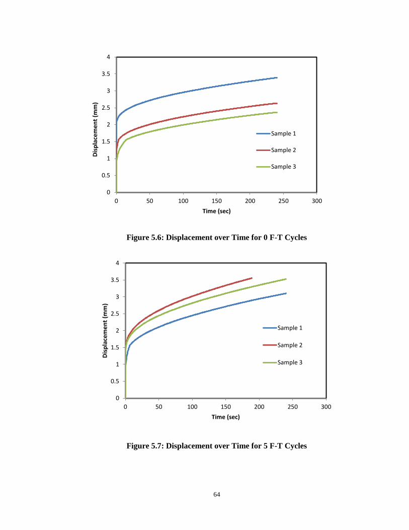
64
Figure 5.6: Displacement over Time for 0 F-T Cycles
Figure 5.7: Displacement over Time for 5 F-T Cycles
0
0.5
1
1.5
2
2.5
3
3.5
4
0 50 100 150 200 250 300
Dis
pla
cem
en
t (m
m)
Time (sec)
Sample 1
Sample 2
Sample 3
0
0.5
1
1.5
2
2.5
3
3.5
4
0 50 100 150 200 250 300
Dis
pla
cem
en
t (m
m)
Time (sec)
Sample 1
Sample 2
Sample 3
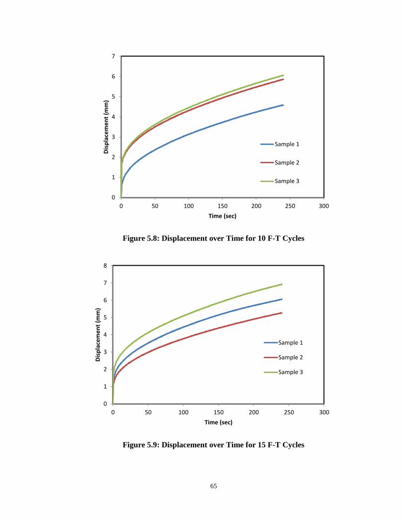
65
Figure 5.8: Displacement over Time for 10 F-T Cycles
Figure 5.9: Displacement over Time for 15 F-T Cycles
0
1
2
3
4
5
6
7
0 50 100 150 200 250 300
Dis
pla
cem
en
t (m
m)
Time (sec)
Sample 1
Sample 2
Sample 3
0
1
2
3
4
5
6
7
8
0 50 100 150 200 250 300
Dis
pla
cem
en
t (m
m)
Time (sec)
Sample 1
Sample 2
Sample 3
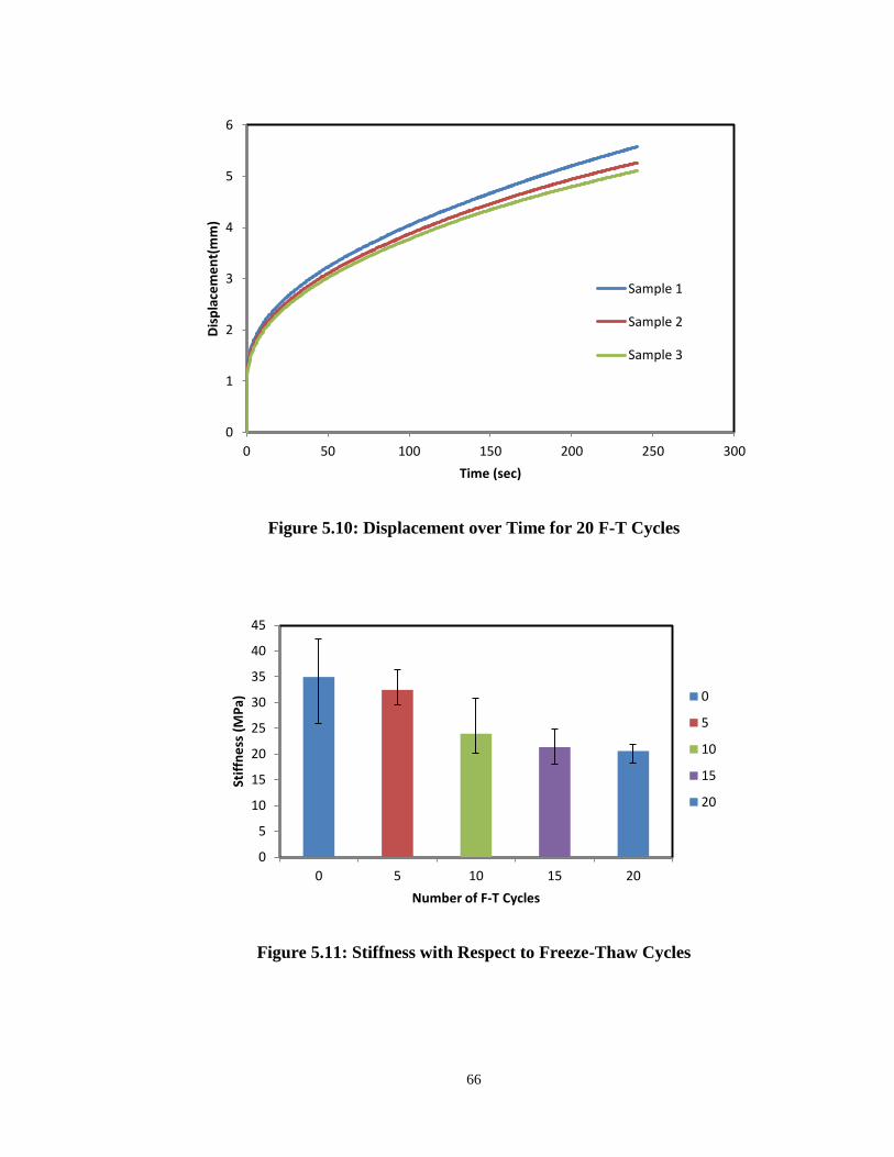
66
Figure 5.10: Displacement over Time for 20 F-T Cycles
Figure 5.11: Stiffness with Respect to Freeze-Thaw Cycles
0
1
2
3
4
5
6
0 50 100 150 200 250 300
Dis
pla
cem
en
t(m
m)
Time (sec)
Sample 1
Sample 2
Sample 3
0
5
10
15
20
25
30
35
40
45
0 5 10 15 20
Stif
fne
ss (
MP
a)
Number of F-T Cycles
0
5
10
15
20

67
The creep test data is introduced into the equation to obtain flexural creep stiffness at -
10°C and for m-value of the stiffness vs. logarithmic time is plotted to obtain the slope at
any specific time. Figure 5.12 shows the plot of stiffness vs. logarithmic time for m-value
or slope calculation for 60 sec. According to stiffness value is calculated for 60 sec for
each sample. Three samples for each class of freeze-thaw cycles are analyzed and plotted
for statistical analysis, as shown figure 5.13. The box plot for each class show median, ¼
quartile, ¾ quartile, and variation range of the data. The figure shows the stiffness
decreases with increase in freeze-thaw cycle. Therefore, the freeze-thaw cycle is
decreasing the stiffness of the material and increasing the damage in the sample. In
addition, control sample and 10 cycles freeze-thaw damaged data shows higher variation
of data among themselves. Stiffness data for each class freeze-thaw cycle analyzed
further for ANOVA analysis. However, the data needs to be analyzed for normality
assumption for further analysis. Data analysis is done in statistical software R. For
normality assumption, the regression residuals are introduced for Shapiro Wilk test. The
analysis shows a p-value of 0.09876 which is greater than 0.05, therefore there is not
enough evidence to show that the data does not hold normality assumption. Further, all
the data for different freeze-thaw cycles shows a p-value of 0.019822, which is less than
0.05. Therefore, there is enough evidence that the mean of each sample class is different
from each other. Doing further statistical analysis, using a t-test with 95% confidence
interval, it is shown that a statistical difference is seen after 20 freeze-thaw cycle. It can
be said, damage accumulates during the first few cycles of freeze-thaw and after 20
cycles, freeze-thaw has a clear effect on the stiffness of the binder.
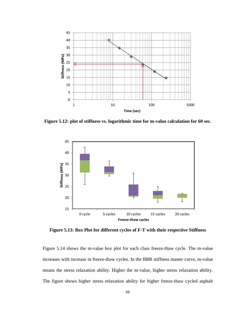
68
Figure 5.12: plot of stiffness vs. logarithmic time for m-value calculation for 60 sec.
Figure 5.13: Box Plot for different cycles of F-T with their respective Stiffness
Figure 5.14 shows the m-value box plot for each class freeze-thaw cycle. The m-value
increases with increase in freeze-thaw cycles. In the BBR stiffness master curve, m-value
means the stress relaxation ability. Higher the m-value, higher stress relaxation ability.
The figure shows higher stress relaxation ability for higher freeze-thaw cycled asphalt
0
5
10
15
20
25
30
35
40
45
1 10 100 1000
Stif
fne
ss (
MP
a)
Time (sec)
15
20
25
30
35
40
45
0 cycle 5 cycles 10 cycles 15 cycles 20 cycles
Stif
fne
ss (
MP
a)
Freeze-thaw cycles
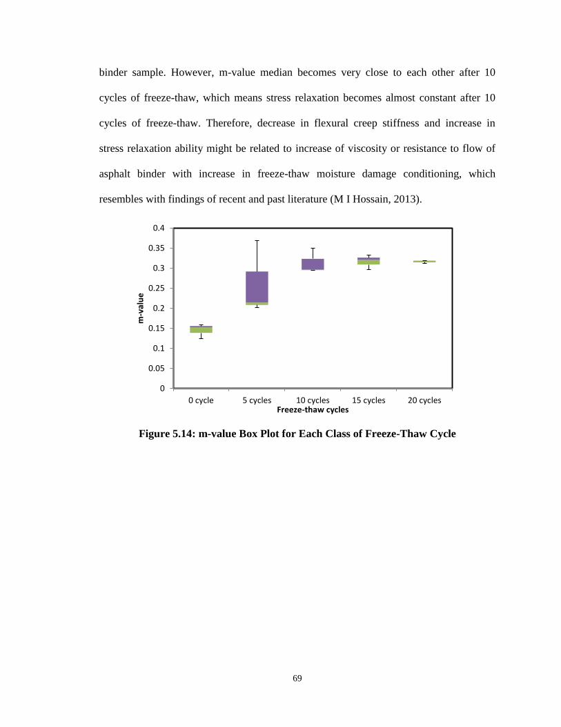
69
binder sample. However, m-value median becomes very close to each other after 10
cycles of freeze-thaw, which means stress relaxation becomes almost constant after 10
cycles of freeze-thaw. Therefore, decrease in flexural creep stiffness and increase in
stress relaxation ability might be related to increase of viscosity or resistance to flow of
asphalt binder with increase in freeze-thaw moisture damage conditioning, which
resembles with findings of recent and past literature (M I Hossain, 2013).
Figure 5.14: m-value Box Plot for Each Class of Freeze-Thaw Cycle
0
0.05
0.1
0.15
0.2
0.25
0.3
0.35
0.4
0 cycle 5 cycles 10 cycles 15 cycles 20 cycles
m-v
alu
e
Freeze-thaw cycles

70
Table 5.4: Stiffness and m-value Test Results for BBR
Stiffness (MPa) m-value
Control Sample
25.8273 21.7836
36.583 21.6341
42.4156 18.2838
5 Cycles Freeze-thaw
31.381 0.202243
29.5504 0.369077
36.4039 0.214423
10 Cycles Freeze-thaw
30.9002 0.350773
20.8413 0.296275
20.0666 0.293994
15 Cycles Freeze-thaw
21.0729 0.320713
24.9219 0.332235
18.0129 0.297421
20 Cycles Freeze-thaw
21.7836 0.318103
21.6341 0.319612
18.2838 0.311261
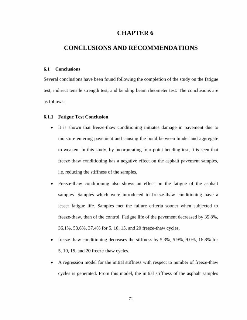
71
6 CHAPTER 6
CONCLUSIONS AND RECOMMENDATIONS
6.1 Conclusions
Several conclusions have been found following the completion of the study on the fatigue
test, indirect tensile strength test, and bending beam rheometer test. The conclusions are
as follows:
6.1.1 Fatigue Test Conclusion
It is shown that freeze-thaw conditioning initiates damage in pavement due to
moisture entering pavement and causing the bond between binder and aggregate
to weaken. In this study, by incorporating four-point bending test, it is seen that
freeze-thaw conditioning has a negative effect on the asphalt pavement samples,
i.e. reducing the stiffness of the samples.
Freeze-thaw conditioning also shows an effect on the fatigue of the asphalt
samples. Samples which were introduced to freeze-thaw conditioning have a
lesser fatigue life. Samples met the failure criteria sooner when subjected to
freeze-thaw, than of the control. Fatigue life of the pavement decreased by 35.8%,
36.1%, 53.6%, 37.4% for 5, 10, 15, and 20 freeze-thaw cycles.
freeze-thaw conditioning decreases the stiffness by 5.3%, 5.9%, 9.0%, 16.8% for
5, 10, 15, and 20 freeze-thaw cycles.
A regression model for the initial stiffness with respect to number of freeze-thaw
cycles is generated. From this model, the initial stiffness of the asphalt samples
72
can be predicted for any number of freeze-thaw cycles when tested at 400µε at
10Hz frequency tested at 20°C. The equation is as follows:
Where,
stiffness, psi
number of freeze-thaw cycles
Additionally, a regression model for the fatigue life of asphalt samples in term of
freeze-thaw cycles is also developed. This model can predict the fatigue life of
asphalt pavement samples when tested at 400µε at 10Hz frequency and 20°C. The
model follows as:
Where,
number of cycles to failure
number of freeze-thaw cycles
6.1.2 IDT Test Conclusion
Statistically, freeze-thaw conditioning does not have a clear effect on the tensile
strength of asphalt pavement. A decreasing tend can be seen in the strength, but
there is not enough evidence to conclude that freeze-thaw reduces the strength
given the number of samples tested and the confidence interval.
73
6.1.3 BBR Test Conclusion
Freeze-thaw cycles for inducing moisture damage in asphalt binder decrease the
thermal stiffness or thermal stress capacity of asphalt binder.
Increase in freeze-thaw cycle increases m-value obtained from stiffness master
curve. The increase in m-value means increase in stress relaxation ability of
asphalt binder, which might be related to increase of viscosity of asphalt binder
for moisture damage.
Flexural creep stiffness of asphalt binder decreases with increase in freeze-thaw
cycles. Stiffness decreased by 7.1%, 31.5%, 38.9%, and 41.1% for 5, 10, 15, and
20 freeze-thaw cycles
6.2 Recommendations for Future Work
Currently, cylindrical dynamic modulus test is used to determine dynamic
modulus of asphalt concrete. These values are used in MEPDG for determining
rutting and fatigue. Therefore, fatigue test on cylindrical sample may be thought-
provoking and can be done in the future with similar conditioning methods.
To further investigate into this study, it is recommended to correlate values
attained in the lab to field values.
Furthermore, additional freeze-thaw cycles can be incorporated to determine and
verify the behavior of the asphalt concrete and binder.
Moreover, more extreme cases of weather pattern can be looked at. In Alaska,
weather reaches freezing temperatures as cold as -40°C, it may be of interest to
investigate lower temperature and evaluate damage.
74
REFERNCES
AASHTO T 168-07. Standard Test Method for Sampling Bituminous Paving Mixtures,
American Association of State Highway and Transportation Officials (AASHTO),
Washington D.C., (2007).
AASHTO T 269-07. “Standard Method of Test for Percent Air Voids in Compacted
Dense and Open Asphalt Mixtures.” American Association of State Highway and
Transportation Officials (AASHTO), Washington D.C., (2007).
AASHTO T321-07. “Standard Test Method for Determining the Fatigue Life of
Compacted Hot-Mix Asphalt (HMA) Subjected to Repeated Flexural Bending.”
American Association of State Highway and Transportation Officials (AASHTO),
Washington D.C., (2007).
AASHTO T322-07. “Standard Method of Test for Determining the Creep Compliance
and Strength of Hot-Mix Asphalt (HMA) Using the Indirect Tensile Test Device.”
American Association of State Highway and Transportation Officials (AASHTO),
Washington D.C., (2007).
AASHTO T283-07. “Standard Method of Test for Resistance of Compacted Asphalt
Mixtures to Moisture-Induced Damage.” American Association of State Highway
and Transportation Officials (AASHTO), Washington D.C., (2007).
AASHTO T313-08. “Standard Method of Test for Determining the Flexural Creep
Stiffness of Asphalt Binder Using the Bending Beam Rheometer (BBR).”

75
American Association of State Highway and Transportation Officials (AASHTO),
Washington D.C., (2008).
AASHTO T312-04. “Standard Method of Test for Preparing and Determining the
Density of Hot-Mix Asphalt (HMA) Specimens by Means of the Superpave
Gyratory Compactor." American Association of State Highway and
Transportation Officials (AASHTO), Washington D.C., (2004).
ASTM C666.C666M. “Standard Test Method for Resistance of Concrete to Rapid
Freezing and Thawing.” American Society for Testing and Materials (ASTM),
West Conshohocken, PA., (2008).
ASTM C1645/C1645M. “Standard Test Method for Freeze-thaw and De-icing Salt
Durability of Solid Concrete Interlocking Paving Units” American Society for
Testing and Materials (ASTM), West Conshohocken, PA., (2012).
ASTM D6857/D6857M-11. “Standard Test Method for Maximum Specific Gravity and
Density of Bituminous Paving Mixtures Using Automatic Vacuum Sealing
Method.” American Society for Testing and Materials (ASTM), West
Conshohocken, PA., (2011).
Carpenter, S. H., Ghuzlan, K. A., and Shen, S. (2003). “Fatigue Endurance Limit for
Highway and Airport Pavement.” Transportation Research Record, No. 1832, pp.
131-138.
Dave, E. V., Braham, A. F., Buttlar, W. G., and Paulino, G. H., (2011). “Development of
a Flattened Indirect Tension Test for Asphalt Concrete.” Journal of Testing and
Evaluation, Volume 29, issue 3.
76
Schmidt, R. J., (1974). “Effect of Temperature, Freeze-Thaw, and Various Moisture
Conditions on the Resilient Modulus of Asphalt-Treated Mixes.” Journal of
Transportation Research Record, Volume 480, issue 515, pp. 27-39.
Goh, S. and You, Z., (2012). “Evaluation of Hot-Mix Asphalt Distress under Rapid
Freeze-Thaw Cycles Using Image Processing Technique.” Journal of American
Society of Civil Engineers, volume 12, pp. 3305-3315.
Timm, D. H., Robbins, M. M., Willis, J. R., Tran, N., and Taylor, A. J., (2012).
“Evaluation of Mixture Performance and Structural Capacity of Pavements
Capacity of Pavements Utilizing Shell Thiopave.” National Center for Asphalt
Technology, Construction, Laboratory Evaluation and Full-Scale Testing of
Thiopave® Test Sections – Final Report.
Chen, X., and Huang, B., (2008). “Evaluation of Moisture Damage in Hot Mix Asphalt
Using Simple Performance and Superpave Indirect Tensile Tests.” Journal of
Elsevier, Construction and Building Materials, No. 22, 1950–1962.
Mei, Y., Liang, N., Cao, and Y., Li, Z., (2010). “Fatigue Life Prediction of Asphalt
Pavement Based on Cumulative Damage.” Preceding’s of the Conference,
International Conference on Mechanic Automation and Control Engineering,
Wuhan, pp. 2876-2882.
Coni, M., (2008). “FE Evaluation of 4-point Bending Test for Fatigue Cracking
Assessment.” Pavement Cracking: Mechanisms, Modeling, Detection, Testing
and Case Histories, pp. 271-281.
Feng, D., Yi, J., Wang, L., and Wang, D., (2009). “Impact of Gradation Types on Freeze-
Thaw Performance of Asphalt Mixtures in Seasonal Frozen Region.” Journal of

77
American Society of Civil Engineers, Critical Issues in Transportation Systems
Planning, Development, and Management, pp. 2336-2342.
Feng, D., Yi, J., Wang, L., and Wang, D., (2010). “Impact of salt and freeze–thaw cycles
on performance of asphalt mixtures in coastal frozen region of China.” Journal of
Elsevier, Cold Regions Science and Technology, No 62, pp. 34-41.
Lu, Q., and Harvey, J. T., (2008). “Inclusion of Moisture Effect in Fatigue Test for
Asphalt Pavements.” Transportation and Development Innovative Best Practices
2008: Proceedings of the First International Symposium, China, pp. 511-517.
Liu, Q., Wu, S., and Schlangen, E. (2013). “Induction heating of asphalt mastic for crack
control”. Journal of Elsevier, Cold Regions Science and Technology, No. 41, pp.
345-351.
Özgan, E., and, Serin, S., (2012). “Investigation of certain engineering characteristics of
asphalt concrete exposed to freeze–thaw cycles.” Journal of Elsevier, Cold
Regions Science and Technology.
Shu, X., Huang, B., and Vukosavljevic, D., (2008). “Laboratory evaluation of fatigue
characteristics of recycled asphalt mixture.” Journal of Elsevier, Construction and
Building Materials, No. 22, pp. 1323–1330.
Shu, X., Huang, B., Shrum, E. D., and Jia, X., (2012). “Laboratory evaluation of moisture
susceptibility of foamed warm mix asphalt containing high percentages of
RAP.” Journal of Elsevier, Construction and Building Materials, No. 35, pp.
125-130.
78
Bolzan, P.E., (1989). “Moisture Susceptibility Behavior of Asphalt Concrete and
Emulsified Asphalt Mixtures Using the Freeze-Thaw Padestal Test.”
Transportation Research Record, volume no. 1228, pp. 9-16.
Christensen, D.W., and Bonaquist, R. F., (2004) “Evaluation of Indirect Tensile Test
(IDT) Procedures for Low-Temperature Performance of Hot Mix Asphalt”.
National Cooperative Highway Research Program, Report 530, Washington D.C.
Pan, P., Sun, C., Tang, N., Chen, M., and Wu, S., (2013). “Study on Volume
Performance of Conductive Asphalt Concrete Based on Freeze-thaw Cycle.”
Applied Mechanics and Materials, Vols. 303-306, pp. 2501-2504.
Huang, S., Robertson, R. E., Branthaver. J. F., Petersen, C. J., (2005). “Impact of Lime
Modification of Asphalt and Freeze-Thaw Cycling on the Asphalt-Aggregate
Interaction and Moisture Resistance to Moisture Damage.” Journal of Materials
in Civil Engineering, Vol. 17, No. 6, pp. 711-718.
Poulikakos, L. D., and Partl, M. N., (2009). “Evaluation of Moisture Susceptibility of
Porous Asphalt Concrete Using Water Submersion Fatigue Tests.” Journal of
Elsevier, Construction and Building Materials. No. 23, pp. 3475-3484.
Recommended