MATH1725 Revision Questions
File last updated at 21:13 on May 18, 2015
How this file is arranged
I answer general questions first. These are arranged in date order, with the most recent
questions answered first.
Then I answer questions about the examination past papers starting with the most recent
examination paper (2014) and ending with the oldest examination paper asked about. For
any given examination paper, I answer questions about section A first and then questions
about section B.
General questions
General question: 18/5/2015
Bit last minute but would you be able to explain the differences when testing paired data
vs unpaired data for differences? I understand how to tell which kind of data it is but then
I’m not 100% what the differences in testing the data are.
Response: If paired (matched) data, you form the differences di = xi − yi. You then want
to test H0, whether the mean difference µd equals zero. Thus your test statistic is
t =d
√
s2d/n
which has a tn−1 distribution if H0 is true.
If two independent samples (with unknown variances but known to equal σ2) you use
the test statistic
t =x − y
√
s2 ((1/nx) + (1/ny))
which has a tnx+ny−2 distribution if H0 is true, that the means are equal.
General question: 17/5/2015
I’m several of the past papers we are asked to define what is meant by the “P -value of the
test” and “5% significance level”. Am I right to say the 5% significant level is the probability
of rejecting the null hypothesis when it is true is 0.05. And is the P -value of the test the
probability of X as or more extreme that x observed if null hypothesis is true. I’m not sure
if maybe I’m saying the same thing here.
Response: A 5% significance level means, as you correctly state, that:
pr{Reject H0 when H0 true} = 0.05.
The P -value of the test is essentially the probability of obtaining a value as or more
extreme than the one observed when assuming the null hypothesis is true. Thus if testing
1
H0: µ = 0 against H1: µ > 0, then
P = pr{
|X| > |x| when H0 is true}
.
If testing H0: µ = µ0 against H1: µ 6= µ0, then
P = pr{
|X − µ0| > |x − µ0| when H0 is true}
.
General question: 17/5/2015
A question from a past paper is “Use a chi-squared-goodness-of-fit test to determine whether
the fitted normal distribution gives a good fit to these data”. I was wondering, would I choose
the level of significance myself or would a small chi-squared value (such as 0.551) be enough
to conclude that it is a good fit?
Response: I would expect you to choose a significance level, say 10% or 5% or 1%.
You could report the P -value of the test, but you would need to use a computer (say)
to determine the P -value of your test.
Though a small value of χ2obs would be indicative of accepting a null hypotgesis, strictly
you should do a formal test with pre-specified significance level.
For example, for k = 1 degrees of freedom, χ2obs = 0.551 would correspond to P = 0.4579.
Using R you would have:
1-pchisq(0.551,1) # pchisq command gives cumulative probability.
[1] 0.4579094
General question: 17/5/2015
Am I correct in thinking that rXY and ρXY are the same in principle, but the former is for
a sample and the latter is for a population?
Response: Yes. Sample correlation is rXY . For random variables X and Y , corr(X, Y ) =
ρXY .
General question: 14/5/2015
When do you use z =x − µ
σand when to use z =
x − µ√
σ2/nif that makes sense. I have a
general idea but I recently used the wrong one in a past paper.
Response: If X ∼ N(µ, σ2), then Z =X − µ
σ∼ N(0, 1). Thus pr{X < 1} = pr
{
Z <1 − µ
σ
}
.
If Xi ∼ N(µ, σ2) for i = 1, 2, . . . , n, with the Xi independent, then the mean X satisfies
X ∼ N(µ, σ2/n). In this case Z =X − µ√
σ2/n∼ N(0, 1). Thus pr
{
X < 1}
= pr
{
Z <1 − µ√
σ2/n
}
.
However this latter case is really the same as the former case! For put v2 = σ2/n.
Then you can see that X ∼ N(µ, v2) and so in this case Z =X − µ
v∼ N(0, 1). Thus
pr{
X < 1}
= pr
{
Z <1 − µ
v
}
.
2
Don’t try to learn lots of different formulae. Try to understand the concepts:
(1) Standardization: If X ∼ N(µ, variance=σ2), then Z =X − µ
σ∼ N(0, 1).
(2) Distribution of the mean: If Xiind∼ N(µ, σ2), then X ∼ N(µ, variance=σ2/n).
General question: 21/5/2014
When calculating the sample variance s2, which is more appropriate, the exact value of the
sample mean, like a fraction, or a value rounded to the nearest decimal point?
Response: Consider using the formula
s2 =1
n − 1
(
n∑
i=1
x2i − nx2
)
.
In rounding values of x you need to be aware of rounding errors in your calculations.
As an example, suppose we have n = 9 values 1.1, 1.2, 1.4, 1.5, 1.6, 1.8, 1.9, 2.1, 2.3.
Here9∑
i=1
xi = 14.9, x =1
9
9∑
i=1
xi =14.9
9= 1.65555,
9∑
i=1
x2i = 25.97.
Exactly
s2 =1
8
(
25.97 − 9
(
14.9
9
)2)
= 0.1627777 . . . .
If you use x = 1.65556, you get s2 = 0.1627612, with a relative percentage error
100 × (0.1627612 − 0.1627778)
0.1627778= −0.0102%.
The table below shows what happens when using different values for x.
x s2 Relative percentage error
14.9/9 0.1627778 0.0000 %
1.655556 0.1627751 −0.0010 %
1.65556 0.1627612 −0.0102 %
1.6556 0.1626122 −0.1017 %
1.656 0.1611220 −1.0172 %
1.66 0.1452000 −10.1843 %
1.7 −0.0050000 −103.0717 %
Even in this simple case the message is clear: be very precise in your value for x!
General question: 17/5/2014
I was just wondering if you could tell me what sampling without replacement and testing
homogeneity meant?
Response: Sampling without replacement: Imagine a population of N objects and you
want to sample n of them. Pick one population member. This leaves N − 1 to choose from
3
for the second sample member. Having chosen the second sample member you now have
N − 2 to choose from for the second sample member. And so on.
Sampling with replacement: Imagine a population of N objects and you want to sample
n of them. Pick one population member. Look at it. Replace it into the population. You
now have N to choose from for the second sample member. Look at it. Replace it into the
population. You now have N to choose from for the third sample member. And so on.
Testing homogeneity: covered in lecture 20 for a contingency table with fixed marginal
totals. Suppose you have m rows and n columns with fixed row totals. Hypothesis is of the
form H0:π1,j = π2,j = π3,j = . . . = πm,j(= πj) for j = 1, 2, . . . , n. You are testing whether
the proportions in column j are the same for each row. As an example, suppose we have
three customer surveys in which we sample 100 in the North, 120 in the Midlands, and 110
in the South. Customers can like (1) the product, be indifferent (2), or dislike it (3). We
have three surveys with fixed totals so conduct a test of homogeneity. Our hypothesis is
thus H0:πN,j = πM,j = πS,j(= πj) for j = 1, 2, 3.
General question: 16/5/2014
I am struggling with an aspect of your course, which is finding the 95% confidence intervals.
I do not understand how to get the piece of the formula after the mean ±. I hope this makes
sense. I understand it is to do with the t-tables, but I assumed it was always 1.96?
Response: Recall lecture 4. Here X1, X2, . . . , Xnind∼ N(µ, σ2) with known variance σ2, so
that X ∼ N(µ, σ2/n). Thus
Z =X − µ√
σ2/n∼ N(0, 1).
Since for a standard normal distribution we know that pr{−1.96 < Z < +1.96} = 0.95 this
gives
pr
{
−1.96 <X − µ√
σ2/n< +1.96
}
= 0.95.
This can be re-arranged to give the 95% confidence interval for µ in the form
µ ∈ x ± 1.96√
σ2/n.
Now suppose that the variance σ2 is unknown. Here we estimate σ2 using the sample
variance s2 and we then know that
T =X − µ√
s2/n∼ tn−1.
Since for a tn−1-distribution we know that pr{−tn−1(2.5%) < T < +tn−1(2.5%)} = 0.95 this
gives
pr
{
−tn−1(2.5%) <X − µ√
s2/n< −tn−1(2.5%)
}
= 0.95.
This can be re-arranged to give the 95% confidence interval for µ in the form
µ ∈ x ± tn−1(2.5%)√
s2/n.
4
Notice that in both cases the formula is of the form
point estimate for parameter ± constant × Stdev [point estimate]
where the constant term depends upon the distribution of the point estimate. In the first
case Var[X] = σ2/n and a normal distribution is used. In the second case the estimated
variance is s2/n and this leads to a t-distribution with appropriate degrees of freedom.
General question: 13/5/2013
I’m a bit confused on hypothesis tests. I am working through the worked example questions
in the back of the exercises handout, and on one question the test statistic is Z = (X−µ)/σ
rather than Z = (X − µ)/(σ/√
n) like all the other ones. Why do you not divide by√
n?
I’m guessing it’s to do with the binomial distribution of the data but I’m not sure.
Response: In all cases the test of hypothesis was based on a test statistic U which satisfied
E[U ] = m and Var[U ] = v2. A test of hypothesis about the parameter m would typically be
based on the test statistic Z =U − m
v. If U ∼ N(m, v2), then Z ∼ N(0, 1).
For example, in lecture 5 we had Xiind∼ N(µ, σ2) for i = 1, 2, . . . , n. Then X ∼ N(µ, σ2/n)
so that Z =X − µ√
σ2/n∼ N(0, 1) and this was used to derive test of hypotheses about µ with
σ2 known. Here U = X, m = µ and v2 = σ2/n.
In lecture 6, with variance σ2 unknown, we estimated σ2 using the sample variance s2.
Our test of hypothesis about µ was based on the result T =X − µ√
S2/n∼ tn−1. Here U = X,
m = µ and v2 = S2/n.
In lecture 10 we wanted to test the slope β of a regression line and used the re-
sult β ∼ N
β,σ2
n∑
i=1
(xi − x)2
so that Z =β − β
√
√
√
√
√
√
σ2
n∑
i=1
(xi − x)2
∼ N(0, 1). In practice we have
to estimate σ2 and use the result T =β − β
√
√
√
√
√
√
σ2
n∑
i=1
(xi − x)2
∼ tn−2. Here U = β, m = β,
v2 = σ2
/
n∑
i=1
(xi − x)2.
Similar comments can be made about the tests of hypothesis developed in lectures 15,
16 and 17.
In the worked examples binomial example we observed the number of sizes in 100 throws
of a die and wanted to test if the probability of a six occurring was 1/6. Let X be number
of sixes in n = 100 throws, so X ∼ Bin(n = 100, θ = 1/6) if H0 true. In this case
5
X ≈ N(nθ, nθ(1 − θ)). The test statistic uses Z =X − nθ
√
nθ(1 − θ)≈ N(0, 1). In this form for
the test we have U = X, m = nθ and v2 = nθ(1 − θ).
Suppose in this latter example we wanted to work with proportions X = X/n; then if H0
true we have X ≈ N(θ, θ(1−θ)/n). The test statistic then uses Z =X − θ
√
θ(1 − θ)/n≈ N(0, 1).
In this form for the test we have U = X, m = θ and v2 = θ(1 − θ)/n.
Recall the Bernoulli trial model of MATH1715. If X1, X2, . . . , Xn are independent
Bernoulli random variables taking values 0 or 1 with probability (1− θ) and θ respectively,
then mean µ = E[Xi] = θ, E[X2i ] = θ, variance σ2 = Var[Xi] = θ(1− θ). Their sum satisfies
X = X1 + X2 + · · · + Xn ∼ Bin(n, θ) ≈ N(nθ, nσ2 = nθ(1 − θ)) and their mean X = X/n
satisfies X ≈ N(θ, σ2/n = θ(1 − θ)/n) and the test statistic satisfies =X − θ√
σ2/n≈ N(0, 1).
General question: 10/5/2013
I’m reading over my notes and in lecture 4 (confidence intervals for normal distribution), it
says that for a 95% confidence interval you always use the value 1.96. Is there any way of
working this out or is it just something that you have to remember? I ask because what if
I had to construct a 90% confidence interval. How do you work out which value to use?
Response: The lecture uses the fact that if X1, X2, . . . , Xnind∼ N(µ, σ2), then X ∼ N(µ, σ2/n).
Thus
Z =X − µ√
σ2/n∼ N(0, 1)
for which pr{−1.96 < Z < 1.96} = 0.95 and so giving
pr
{
−1.96 <X − µ√
σ2/n< +1.96
}
= 0.95.
This can be re-arranged to give the 95% confidence interval for µ.
For a 90% confidence interval, you would repeat the lecture but note that
pr{−1.645 < Z < 1.645} = 0.90.
General question: 3/5/2013
I noticed in the answers to Q2 in Exercises I you used coding z = (x−m)/c for the sample
mean and variance. I would like to know why you did this and what are m and c?
Response: Because the mid points x1 were complicated values 2.95, 3.35, 3.75, 4.15 and
so on. Coding makes the numbers simpler to use, so less difficult computationally, and less
likely to make a mistake!
Choose m as class mid point near the centre of the data. Here the class with greatest
frequency was the 4.0-4.3 class with mid-point 4.15, so I chose m = 4.15. Choose c as the
class width, here c = 0.4.
6
The coding z = (x−4.15)/0.4 gives coded values −3, −2, −1 and so on. It is a lot easier
working out, for example,
∑
i
fiz2i = 19(−3)2 + 67(−2)2 + 141(−1)2 + · · ·
than working out
∑
i
fix2i = 19(2.95)2 + 67(3.35)2 + 141(3.75)2 + · · · .
General question: 2/5/2013
I just have a quick question about hypothesis testing. I don’t quite understand it and what
it is used for. Could you just briefly explain because I don’t understand why one would
want to test out different µ values if one already knows the mean for that particular set of
data.
Response: Knowing the sample mean x is not the same as knowing the population mean
µ.
Suppose you want to test whether a new drug has any effect on blood pressure. You
take 10 people and measure their blood pressure. Then you give them the drug and measure
their blood pressure again. Suppose the differences, “before − after”, are:
−0.40 0.35 1.28 − 0.66 − 0.57 − 1.27 0.48 0.69 1.74 0.16.
The sample mean is x = 0.18 and the sample variance is s2 = 0.859.
If the drug really has no effect, then the distribution of all possible observed differences
ought to have a mean µ = 0. If the drug does have an effect, then µ 6= 0. All you have is
the sample mean 0.18.
It looks like the sample mean is close to 0, but could it really be significantly different
from 0? You want to test the hypothesis H0: µ = 0 against the alternative H1: µ 6= 0. If
H0 is true, then the sample mean x can be modelled as coming from a normal distribution
with mean 0 and variance σ2/n where σ2 is the population variance for the differences, and
where n = 10 values. Thus
Z =X
√
σ2/n∼ N(0, 1).
Since you do not know σ2, you estimate it using the sample variance s2 = 0.859. Then
T =X
√
S2/n∼ tn−1.
Here you have observed t =0.18
√
0.859/10= 0.18/0.293 = 0.614. This is close to 0, so you
accept H0.
But suppose your sample mean was x = 0.67. This looks close to 0 too, but is it really
close to 0? Here, if s2 = 0.859 still, then t =0.67
√
0.859/10= 0.67/0.293 = 2.287 which is
quite a long way in the tail of the t9 distribution. You would thus reject H0.
7
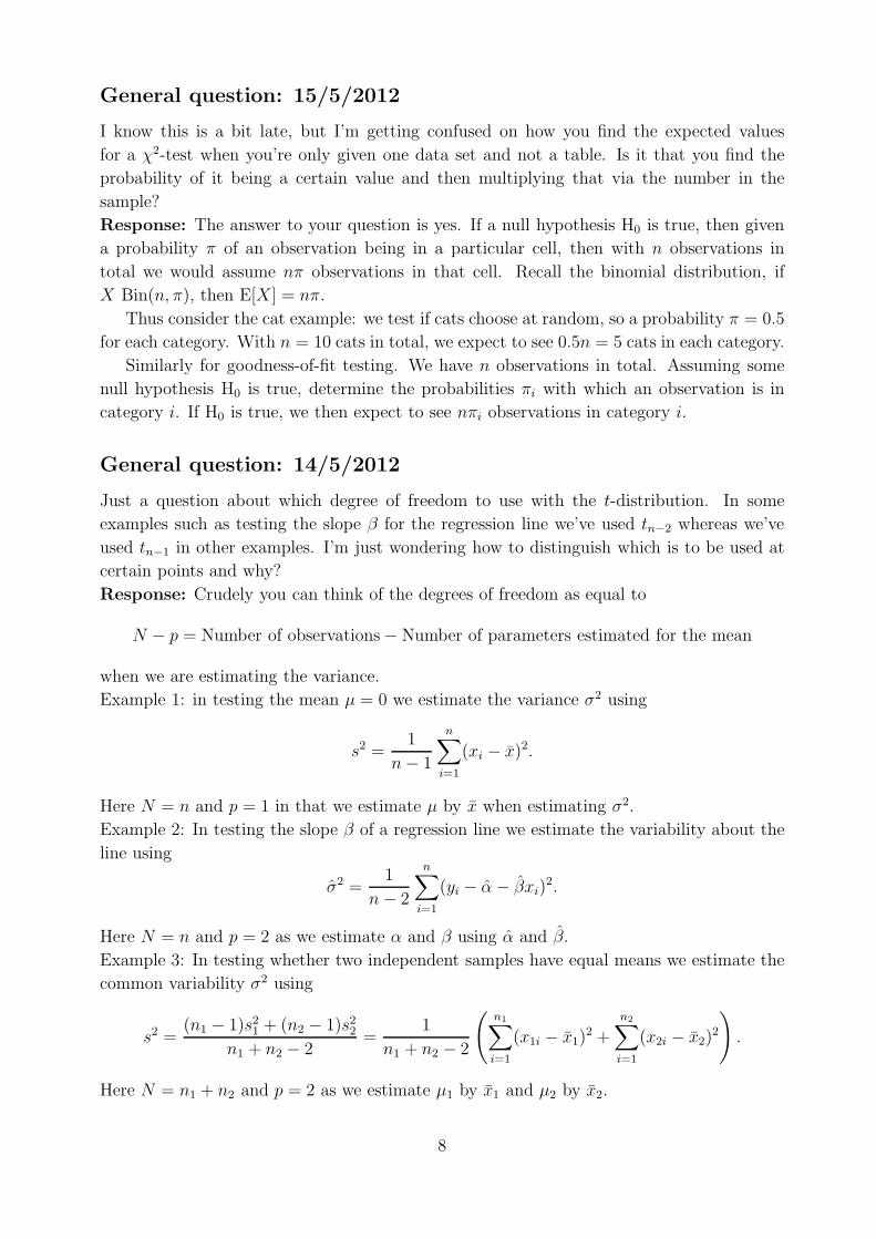
General question: 15/5/2012
I know this is a bit late, but I’m getting confused on how you find the expected values
for a χ2-test when you’re only given one data set and not a table. Is it that you find the
probability of it being a certain value and then multiplying that via the number in the
sample?
Response: The answer to your question is yes. If a null hypothesis H0 is true, then given
a probability π of an observation being in a particular cell, then with n observations in
total we would assume nπ observations in that cell. Recall the binomial distribution, if
X Bin(n, π), then E[X] = nπ.
Thus consider the cat example: we test if cats choose at random, so a probability π = 0.5
for each category. With n = 10 cats in total, we expect to see 0.5n = 5 cats in each category.
Similarly for goodness-of-fit testing. We have n observations in total. Assuming some
null hypothesis H0 is true, determine the probabilities πi with which an observation is in
category i. If H0 is true, we then expect to see nπi observations in category i.
General question: 14/5/2012
Just a question about which degree of freedom to use with the t-distribution. In some
examples such as testing the slope β for the regression line we’ve used tn−2 whereas we’ve
used tn−1 in other examples. I’m just wondering how to distinguish which is to be used at
certain points and why?
Response: Crudely you can think of the degrees of freedom as equal to
N − p = Number of observations − Number of parameters estimated for the mean
when we are estimating the variance.
Example 1: in testing the mean µ = 0 we estimate the variance σ2 using
s2 =1
n − 1
n∑
i=1
(xi − x)2.
Here N = n and p = 1 in that we estimate µ by x when estimating σ2.
Example 2: In testing the slope β of a regression line we estimate the variability about the
line using
σ2 =1
n − 2
n∑
i=1
(yi − α − βxi)2.
Here N = n and p = 2 as we estimate α and β using α and β.
Example 3: In testing whether two independent samples have equal means we estimate the
common variability σ2 using
s2 =(n1 − 1)s2
1 + (n2 − 1)s22
n1 + n2 − 2=
1
n1 + n2 − 2
(
n1∑
i=1
(x1i − x1)2 +
n2∑
i=1
(x2i − x2)2
)
.
Here N = n1 + n2 and p = 2 as we estimate µ1 by x1 and µ2 by x2.
8
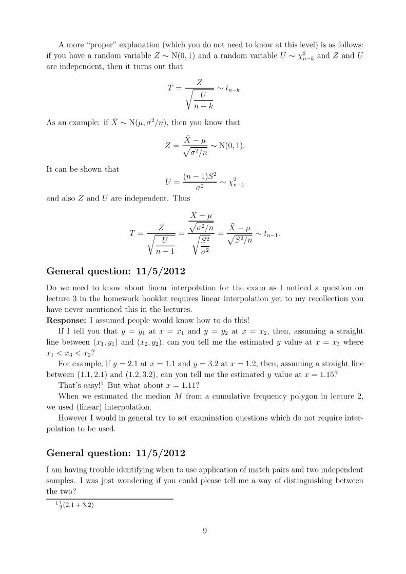
A more “proper” explanation (which you do not need to know at this level) is as follows:
if you have a random variable Z ∼ N(0, 1) and a random variable U ∼ χ2n−k and Z and U
are independent, then it turns out that
T =Z
√
U
n − k
∼ tn−k.
As an example: if X ∼ N(µ, σ2/n), then you know that
Z =X − µ√
σ2/n∼ N(0, 1).
It can be shown that
U =(n − 1)S2
σ2∼ χ2
n−1
and also Z and U are independent. Thus
T =Z
√
U
n − 1
=
X − µ√
σ2/n√
S2
σ2
=X − µ√
S2/n∼ tn−1.
General question: 11/5/2012
Do we need to know about linear interpolation for the exam as I noticed a question on
lecture 3 in the homework booklet requires linear interpolation yet to my recollection you
have never mentioned this in the lectures.
Response: I assumed people would know how to do this!
If I tell you that y = y1 at x = x1 and y = y2 at x = x2, then, assuming a straight
line between (x1, y1) and (x2, y2), can you tell me the estimated y value at x = x3 where
x1 < x3 < x2?
For example, if y = 2.1 at x = 1.1 and y = 3.2 at x = 1.2, then, assuming a straight line
between (1.1, 2.1) and (1.2, 3.2), can you tell me the estimated y value at x = 1.15?
That’s easy!1 But what about x = 1.11?
When we estimated the median M from a cumulative frequency polygon in lecture 2,
we used (linear) interpolation.
However I would in general try to set examination questions which do not require inter-
polation to be used.
General question: 11/5/2012
I am having trouble identifying when to use application of match pairs and two independent
samples. I was just wondering if you could please tell me a way of distinguishing between
the two?
1 1
2(2.1 + 3.2)
9
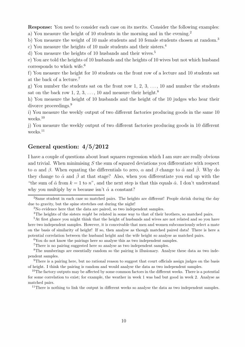
Response: You need to consider each case on its merits. Consider the following examples:
a) You measure the height of 10 students in the morning and in the evening.2
b) You measure the weight of 10 male students and 10 female students chosen at random.3
c) You measure the heights of 10 male students and their sisters.4
d) You measure the heights of 10 husbands and their wives.5
e) You are told the heights of 10 husbands and the heights of 10 wives but not which husband
corresponds to which wife.6
f) You measure the height for 10 students on the front row of a lecture and 10 students sat
at the back of a lecture.7
g) You number the students sat on the front row 1, 2, 3, . . . , 10 and number the students
sat on the back row 1, 2, 3, . . . , 10 and measure their height.8
h) You measure the height of 10 husbands and the height of the 10 judges who hear their
divorce proceedings.9
i) You measure the weekly output of two different factories producing goods in the same 10
weeks.10
j) You measure the weekly output of two different factories producing goods in 10 different
weeks.11
General question: 4/5/2012
I have a couple of questions about least squares regression which I am sure are really obvious
and trivial. When minimising S the sum of squared deviations you differentiate with respect
to α and β. When equating the differentials to zero, α and β change to α and β. Why do
they change to α and β at that stage? Also, when you differentiate you end up with the
“the sum of α from k = 1 to n”, and the next step is that this equals α. I don’t understand
why you multiply by n because isn’t α a constant?
2Same student in each case so matched pairs. The heights are different! People shrink during the day
due to gravity, but the spine stretches out during the night!3No evidence here that the data are paired, so two independent samples.4The heights of the sisters might be related in some way to that of their brothers, so matched pairs.5At first glance you might think that the height of husbands and wives are not related and so you have
here two independent samples. However, it is conceivable that men and women subconsciously select a mate
on the basis of similarity of height! If so, then analyse as though matched paired data! There is here a
potential correlation between the husband height and the wife height so analyse as matched pairs.6You do not know the pairings here so analyse this as two independent samples.7There is no pairing suggested here so analyse as two independent samples.8The numberings are essentially random so the pairing is illusionary. Analyse these data as two inde-
pendent samples.9There is a pairing here, but no rational reason to suggest that court officials assign judges on the basis
of height. I think the pairing is random and would analyse the data as two independent samples.10The factory outputs may be affected by some common factors in the different weeks. There is a potential
for some correlation to exist; for example, the weather in week 1 was bad but good in week 2. Analyse as
matched pairs.11There is nothing to link the output in different weeks so analyse the data as two independent samples.
10
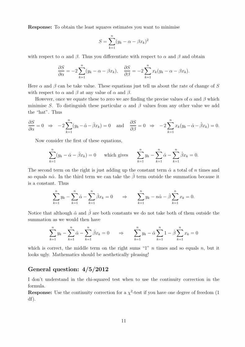
Response: To obtain the least squares estimates you want to minimise
S =
n∑
k=1
(yk − α − βxk)2
with respect to α and β. Thus you differentiate with respect to α and β and obtain
∂S
∂α= −2
n∑
k=1
(yk − α − βxk),∂S
∂β= −2
n∑
k=1
xk(yk − α − βxk).
Here α and β can be take value. These equations just tell us about the rate of change of S
with respect to α and β at any value of α and β.
However, once we equate these to zero we are finding the precise values of α and β which
minimise S. To distinguish these particular α and β values from any other value we add
the “hat”. Thus
∂S
∂α= 0 ⇒ −2
n∑
k=1
(yk − α− βxk) = 0 and∂S
∂β= 0 ⇒ −2
n∑
k=1
xk(yk − α− βxk) = 0.
Now consider the first of these equations,
n∑
k=1
(yk − α − βxk) = 0 which givesn∑
k=1
yk −n∑
k=1
α −n∑
k=1
βxk = 0.
The second term on the right is just adding up the constant term α a total of n times and
so equals nα. In the third term we can take the β term outside the summation because it
is a constant. Thus
n∑
k=1
yk −n∑
k=1
α −n∑
k=1
βxk = 0 ⇒n∑
k=1
yk − nα − β
n∑
k=1
xk = 0.
Notice that although α and β are both constants we do not take both of them outside the
summation as we would then have
n∑
k=1
yk −n∑
k=1
α −n∑
k=1
βxk = 0 ⇒n∑
k=1
yk − αn∑
k=1
1 − βn∑
k=1
xk = 0
which is correct, the middle term on the right sums “1” n times and so equals n, but it
looks ugly. Mathematics should be aesthetically pleasing!
General question: 4/5/2012
I don’t understand in the chi-squared test when to use the continuity correction in the
formula.
Response: Use the continuity correction for a χ2-test if you have one degree of freedom (1
df).
11
General question: 23/4/2011
I don’t know how to differentiate
S =n∑
k=1
(yk − α − βxk)2
for the least squares method.
Response: Recall what you know about differentiation. Thus
∂
∂α
{
n∑
k=1
(yk − α − βxk)2
}
=n∑
k=1
∂
∂α
{
(yk − α − βxk)2}
.
Also∂
∂α
{
(yk − α − βxk)2}
= 2(yk − α − βxk)∂
∂α{(yk − α − βxk)}
using the “chain-rule”.
Similarly you can differentiate with respect to β.
12
2013 Examination paper
2013 exam, question A14: 10/5/2015
Can I answer this question as “when P -value is large, then the null hypothesis H0 is ac-
cepted”?
Response: Yes.
2013 exam, question A15: 18/5/2015
I kindly request you to help me with June 2013 A15 MATH1725 please?
Response: Look at the handout for lecture 10 which introduced residuals.
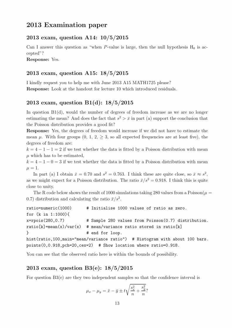
2013 exam, question B1(d): 18/5/2015
In question B1(d), would the number of degrees of freedom increase as we are no longer
estimating the mean? And does the fact that s2 > x in part (a) support the conclusion that
the Poisson distribution provides a good fit?
Response: Yes, the degrees of freedom would increase if we did not have to estimate the
mean µ. With four groups (0, 1, 2, ≥ 3, so all expected frequencies are at least five), the
degrees of freedom are:
k = 4 − 1 − 1 = 2 if we test whether the data is fitted by a Poisson distribution with mean
µ which has to be estimated,
k = 4 − 1 − 0 = 3 if we test whether the data is fitted by a Poisson distribution with mean
µ = 1.
In part (a) I obtain x = 0.70 and s2 = 0.763. I think these are quite close, so x ≈ s2,
as we might expect for a Poisson distribution. The ratio x/s2 = 0.918. I think this is quite
close to unity.
The R code below shows the result of 1000 simulations taking 280 values from a Poisson(µ =
0.7) distribution and calculating the ratio x/s2.
ratio=numeric(1000) # Initialise 1000 values of ratio as zero.
for (k in 1:1000){
x=rpois(280,0.7) # Sample 280 values from Poisson(0.7) distribution.
ratio[k]=mean(x)/var(x) # mean/variance ratio stored in ratio[k]
} # end for loop.
hist(ratio,100,main="mean/variance ratio") # Histogram with about 100 bars.
points(0,0.918,pch=20,cex=2) # Show location where ratio=0.918.
You can see that the observed ratio here is within the bounds of possibility.
2013 exam, question B3(e): 18/5/2015
For question B3(e) are they two independent samples so that the confidence interval is
µx − µy = x − y ± t
√
s2x
n+
s2y
n?
13
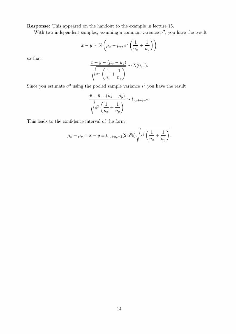
Response: This appeared on the handout to the example in lecture 15.
With two independent samples, assuming a common variance σ2, you have the result
x − y ∼ N
(
µx − µy, σ2
(
1
nx
+1
ny
))
so thatx − y − (µx − µy)√
σ2
(
1
nx
+1
ny
)
∼ N(0, 1).
Since you estimate σ2 using the pooled sample variance s2 you have the result
x − y − (µx − µy)√
s2
(
1
nx
+1
ny
)
∼ tnx+ny−2.
This leads to the confidence interval of the form
µx − µy = x − y ± tnx+ny−2(2.5%)
√
s2
(
1
nx
+1
ny
)
.
14
2012 Examination paper
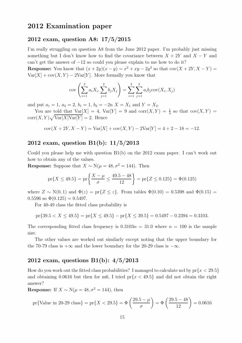
2012 exam, question A8: 17/5/2015
I’m really struggling on question A8 from the June 2012 paper. I’m probably just missing
something but I don’t know how to find the covariance between X + 2Y and X − Y and
can’t get the answer of −12 so could you please explain to me how to do it?
Response: You know that (x + 2y)(x− y) = x2 + xy − 2y2 so that cov(X + 2Y, X − Y ) =
Var[X] + cov(X, Y ) − 2Var[Y ]. More formally you know that
cov
(
2∑
i=1
aiXi,2∑
j=1
bjXj
)
=2∑
i=1
2∑
j=1
aibjcov(Xi, Xj)
and put a1 = 1, a2 = 2, b1 = 1, b2 = −2n X = X1 and Y = X2.
You are told that Var[X] = 4, Var[Y ] = 9 and corr(X, Y ) = 1
3so that cov(X, Y ) =
corr(X, Y )√
Var[X]Var[Y ] = 2. Hence
cov(X + 2Y, X − Y ) = Var[X] + cov(X, Y ) − 2Var[Y ] = 4 + 2 − 18 = −12.
2012 exam, question B1(b): 11/5/2013
Could you please help me with question B1(b) on the 2012 exam paper. I can’t work out
how to obtain any of the values.
Response: Suppose that X ∼ N(µ = 48, σ2 = 144). Then
pr{X ≤ 49.5} = pr
{
X − µ
σ≤ 49.5 − 48
12
}
= pr{Z ≤ 0.125} = Φ(0.125)
where Z ∼ N(0, 1) and Φ(z) = pr{Z ≤ z}. From tables Φ(0.10) = 0.5398 and Φ(0.15) =
0.5596 so Φ(0.125) = 0.5497.
For 40-49 class the fitted class probability is
pr{39.5 < X ≤ 49.5} = pr{X ≤ 49.5} − pr{X ≤ 39.5} = 0.5497 − 0.2394 = 0.3103.
The corresponding fitted class frequency is 0.3103n = 31.0 where n = 100 is the sample
size.
The other values are worked out similarly except noting that the upper boundary for
the 70-79 class is +∞ and the lower boundary for the 20-29 class is −∞.
2012 exam, questions B1(b): 4/5/2013
How do you work out the fitted class probabilities? I managed to calculate m4 by pr{x < 29.5}and obtaining 0.0616 but then for m6, I tried pr{x < 49.5} and did not obtain the right
answer?
Response: If X ∼ N(µ = 48, σ2 = 144), then
pr{Value in 20-29 class} = pr{X < 29.5} = Φ
(
29.5 − µ
σ
)
= Φ
(
29.5 − 48
12
)
= 0.0616
15
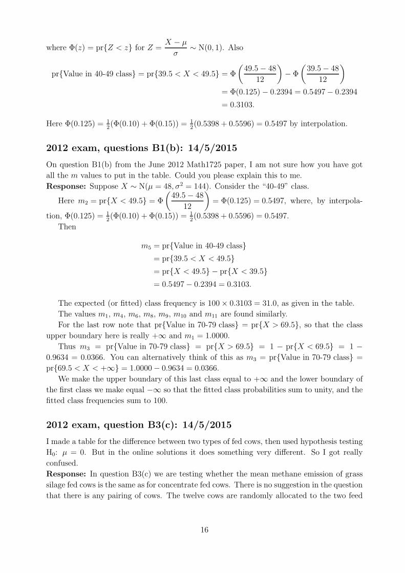
where Φ(z) = pr{Z < z} for Z =X − µ
σ∼ N(0, 1). Also
pr{Value in 40-49 class} = pr{39.5 < X < 49.5} = Φ
(
49.5 − 48
12
)
− Φ
(
39.5 − 48
12
)
= Φ(0.125) − 0.2394 = 0.5497 − 0.2394
= 0.3103.
Here Φ(0.125) = 1
2(Φ(0.10) + Φ(0.15)) = 1
2(0.5398 + 0.5596) = 0.5497 by interpolation.
2012 exam, questions B1(b): 14/5/2015
On question B1(b) from the June 2012 Math1725 paper, I am not sure how you have got
all the m values to put in the table. Could you please explain this to me.
Response: Suppose X ∼ N(µ = 48, σ2 = 144). Consider the “40-49” class.
Here m2 = pr{X < 49.5} = Φ
(
49.5 − 48
12
)
= Φ(0.125) = 0.5497, where, by interpola-
tion, Φ(0.125) = 1
2(Φ(0.10) + Φ(0.15)) = 1
2(0.5398 + 0.5596) = 0.5497.
Then
m5 = pr{Value in 40-49 class}= pr{39.5 < X < 49.5}= pr{X < 49.5} − pr{X < 39.5}= 0.5497 − 0.2394 = 0.3103.
The expected (or fitted) class frequency is 100 × 0.3103 = 31.0, as given in the table.
The values m1, m4, m6, m8, m9, m10 and m11 are found similarly.
For the last row note that pr{Value in 70-79 class} = pr{X > 69.5}, so that the class
upper boundary here is really +∞ and m1 = 1.0000.
Thus m3 = pr{Value in 70-79 class} = pr{X > 69.5} = 1 − pr{X < 69.5} = 1 −0.9634 = 0.0366. You can alternatively think of this as m3 = pr{Value in 70-79 class} =
pr{69.5 < X < +∞} = 1.0000 − 0.9634 = 0.0366.
We make the upper boundary of this last class equal to +∞ and the lower boundary of
the first class we make equal −∞ so that the fitted class probabilities sum to unity, and the
fitted class frequencies sum to 100.
2012 exam, question B3(c): 14/5/2015
I made a table for the difference between two types of fed cows, then used hypothesis testing
H0: µ = 0. But in the online solutions it does something very different. So I got really
confused.
Response: In question B3(c) we are testing whether the mean methane emission of grass
silage fed cows is the same as for concentrate fed cows. There is no suggestion in the question
that there is any pairing of cows. The twelve cows are randomly allocated to the two feed
16
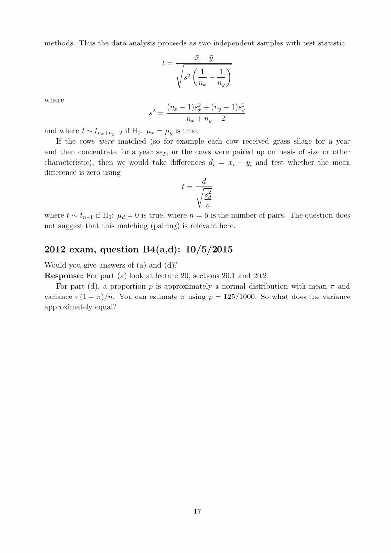
methods. Thus the data analysis proceeds as two independent samples with test statistic
t =x − y
√
s2
(
1
nx
+1
ny
)
where
s2 =(nx − 1)s2
x + (ny − 1)s2y
nx + ny − 2
and where t ∼ tnx+ny−2 if H0: µx = µy is true.
If the cows were matched (so for example each cow received grass silage for a year
and then concentrate for a year say, or the cows were paired up on basis of size or other
characteristic), then we would take differences di = xi − yi and test whether the mean
difference is zero using
t =d√
s2d
n
where t ∼ tn−1 if H0: µd = 0 is true, where n = 6 is the number of pairs. The question does
not suggest that this matching (pairing) is relevant here.
2012 exam, question B4(a,d): 10/5/2015
Would you give answers of (a) and (d)?
Response: For part (a) look at lecture 20, sections 20.1 and 20.2.
For part (d), a proportion p is approximately a normal distribution with mean π and
variance π(1 − π)/n. You can estimate π using p = 125/1000. So what does the variance
approximately equal?
17
2011 Examination paper
2011 exam, questions A8-A10: 14/5/2014
I’m having some trouble with some questions on the May/June 2011 MATH1725 past paper.
In particular:
A8. If a random variable X has a chi-squared distribution with 5 degrees of freedom, what
is the value of x such that pr{X > x} = 0.10?
A9. Suppose that X and Y are independent random variables and have a common binomial
distribution with index n and parameter π. What is the variance of X − Y ?
A10. If X1, X2, . . . , Xn are independent observations from a Bin(n, π) distribution, what is
the variance of their sum, S = X1 + X2 + · · · + Xn?
Response: In A8 you use χ2-tables to look up pr{X > χ25(10%)} = 0.10; see lecture 18.
In A9 you know X and Y are independent so Var[X − Y ] = Var[X] + Var[Y ]. If
X ∼ Bin(n, π), you know from MATH1715 (and lectures 16 and 17) that Var[X] = nπ(1−π).
As Y has the same distribution you know the variance of Y so you can deduce Var[X − Y ].
In A10 if Var[Xi] = σ2 for all i, you know from lecture 14 that Var[X1 +X2 + · · ·+Xn] =
nσ2 as the Xi are mutually independent. Since Xi ∼ Bin(n, π) then Var[Xi] = nπ(1 − π)
and you can deduce the variance of S.
2011 exam, question B1(c-iii): 11/5/2012
Would it be possible to get solutions from 2011 past paper on how to find the test statistic
for B1 (c-iii).
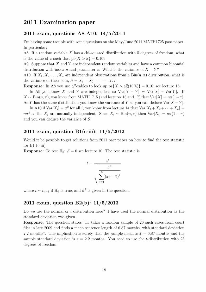
Response: To test H0: β = 0 see lecture 10. The test statistic is
t =β
√
√
√
√
√
√
σ2
n∑
i=1
(xi − x)2
where t ∼ tn−1 if H0 is true, and σ2 is given in the question.
2011 exam, question B2(b): 11/5/2013
Do we use the normal or t-distribution here? I have used the normal distribution as the
standard deviation was given.
Response: The question states “he takes a random sample of 26 such cases from court
files in late 2009 and finds a mean sentence length of 6.87 months, with standard deviation
2.2 months”. The implication is surely that the sample mean is x = 6.87 months and the
sample standard deviation is s = 2.2 months. You need to use the t-distribution with 25
degrees of freedom.
18
2011 exam, question B2(e): 16/5/2015
In the revision answers you have said that sy = 1.1 months. Should it not be 1.21 months
as 2.22 × 0.52 = 1.21?
Response: Standard deviation of sentence length X is sx = 2.2. Variance of sentence
length is s2x = 2.22.
In part (d) we are told to suppose that people spend 50% of their sentence in prison.
If Y is the time spent in prison and X is the sentence length, then Y = 0.50X. Thus
Var[Y ] = Var[0.50X] = 0.52Var[X] = 1.21. Thus Stdev(Y ) =√
1.21 = 1.1.
2011 exam, question B2(e): 11/5/2013
Do we use the normal or t-distribution here? I have used the normal distribution as the
standard deviation was given.
Response: The question states “he takes a random sample of 26 such cases from court
files in late 2009 and finds a mean sentence length of 6.87 months, with standard deviation
2.2 months”. The time in prison y is 50% of the sentence length x so in this case we have
sample mean y = 3.435 months and the sample standard deviation is sy = 1.1 months. You
again need to use the t-distribution with 25 degrees of freedom.
2011 exam, question B2(e): 11/5/2012
Would it be possible to get solutions from 2011 past paper on how to find the test statistic
for B2 (e).
Response: We test H0: µ = 5 against H1: µ < 5 using a t-statistic as in lecture 5.
2011 exam, question B3(c): 21/5/2014
I am not sure about the answer in B3(c).
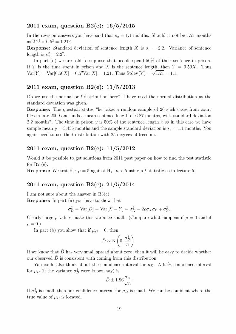
Response: In part (a) you have to show that
σ2D = Var[D] = Var[X − Y ] = σ2
X − 2ρσXσY + σ2Y .
Clearly large ρ values make this variance small. (Compare what happens if ρ = 1 and if
ρ = 0.)
In part (b) you show that if µD = 0, then
D ∼ N
(
0,σ2
D
n
)
.
If we know that D has very small spread about zero, then it will be easy to decide whether
our observed D is consistent with coming from this distribution.
You could also think about the confidence interval for µD. A 95% confidence interval
for µD (if the variance σ2D were known say) is
D ± 1.96σD√
n.
If σ2D is small, then our confidence interval for µD is small. We can be confident where the
true value of µD is located.
19
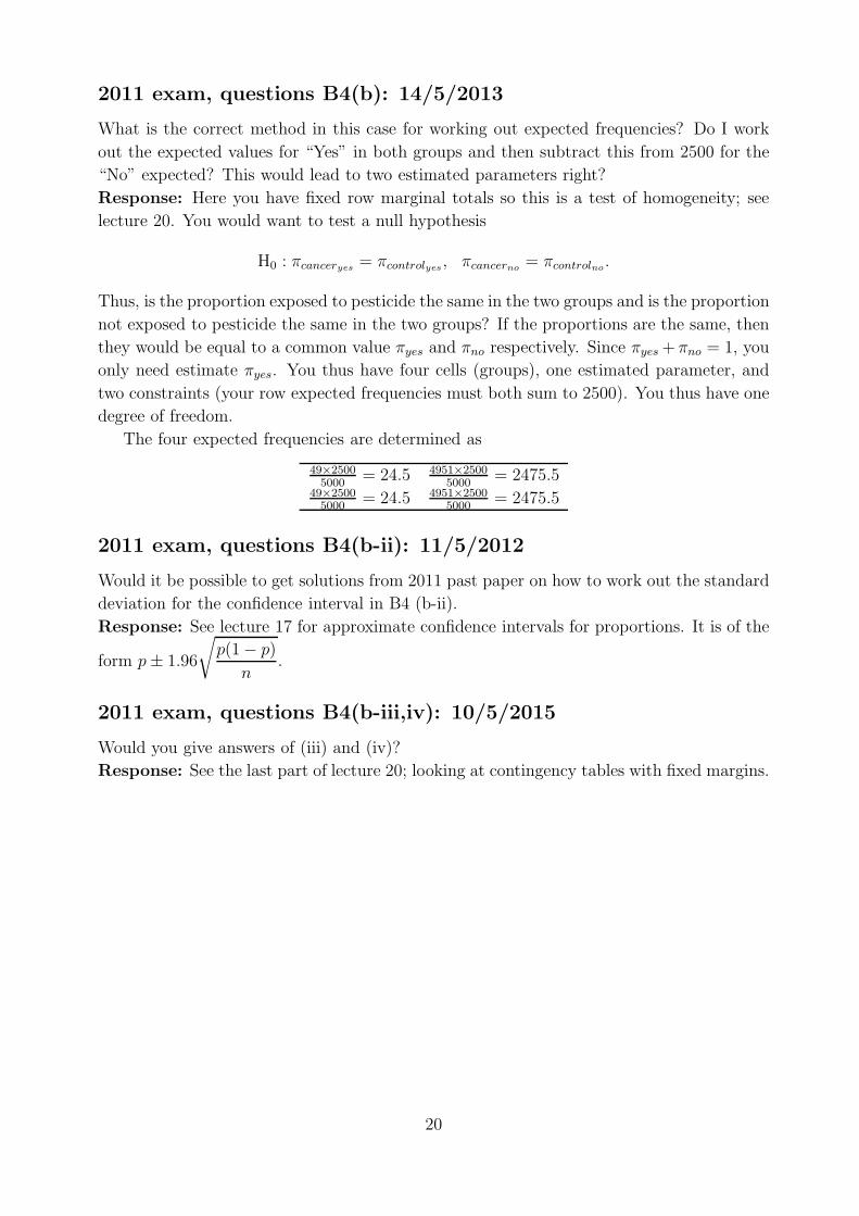
2011 exam, questions B4(b): 14/5/2013
What is the correct method in this case for working out expected frequencies? Do I work
out the expected values for “Yes” in both groups and then subtract this from 2500 for the
“No” expected? This would lead to two estimated parameters right?
Response: Here you have fixed row marginal totals so this is a test of homogeneity; see
lecture 20. You would want to test a null hypothesis
H0 : πcanceryes= πcontrolyes
, πcancerno= πcontrolno
.
Thus, is the proportion exposed to pesticide the same in the two groups and is the proportion
not exposed to pesticide the same in the two groups? If the proportions are the same, then
they would be equal to a common value πyes and πno respectively. Since πyes + πno = 1, you
only need estimate πyes. You thus have four cells (groups), one estimated parameter, and
two constraints (your row expected frequencies must both sum to 2500). You thus have one
degree of freedom.
The four expected frequencies are determined as
49×2500
5000= 24.5 4951×2500
5000= 2475.5
49×2500
5000= 24.5 4951×2500
5000= 2475.5
2011 exam, questions B4(b-ii): 11/5/2012
Would it be possible to get solutions from 2011 past paper on how to work out the standard
deviation for the confidence interval in B4 (b-ii).
Response: See lecture 17 for approximate confidence intervals for proportions. It is of the
form p ± 1.96
√
p(1 − p)
n.
2011 exam, questions B4(b-iii,iv): 10/5/2015
Would you give answers of (iii) and (iv)?
Response: See the last part of lecture 20; looking at contingency tables with fixed margins.
20
2010 Examination paper
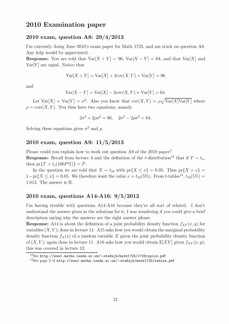
2010 exam, question A8: 29/4/2013
I’m currently doing June 2010’s exam paper for Math 1725, and am stuck on question A8.
Any help would be appreciated.
Response: You are told that Var[X + Y ] = 96, Var[X − Y ] = 64, and that Var[X] and
Var[Y ] are equal. Notice that
Var[X + Y ] = Var[X] + 2cov(X, Y ) + Var[Y ] = 96
and
Var[X − Y ] = Var[X] − 2cov(X, Y ) + Var[Y ] = 64.
Let Var[X] = Var[Y ] = σ2. Also you know that cov(X, Y ) = ρ√
Var[X]Var[Y ] where
ρ = corr(X, Y ). You thus have two equations, namely
2σ2 + 2ρσ2 = 96, 2σ2 − 2ρσ2 = 64.
Solving these equations gives σ2 and ρ.
2010 exam, question A9: 11/5/2013
Please could you explain how to work out question A9 of the 2010 paper?
Response: Recall from lecture 4 and the definition of the t-distribution12 that if T ∼ tν ,
then pr{T > tν(100P%)} = P .
In the question we are told that X ∼ t10 with pr{X ≤ x} = 0.95. Thus pr{X > x} =
1−pr{X ≤ x} = 0.05. We therefore want the value x = t10(5%). From t-tables13, t10(5%) =
1.812. The answer is B.
2010 exam, questions A14-A16: 9/5/2012
I’m having trouble with questions A14-A16 because they’re all sort of related. I don’t
understand the answer given in the solutions for it, I was wondering if you could give a brief
description saying why the answers are the right answer please.
Response: A14 is about the definition of a joint probability density function fXY (x, y) for
variables (X, Y ); done in lecture 11. A15 asks how you would obtain the marginal probability
density function fX(x) of a random variable X given the joint probability density function
of (X, Y ); again done in lecture 11. A16 asks how you would obtain E[XY ] given fXY (x, y);
this was covered in lecture 12.
12See http://www1.maths.leeds.ac.uk/∼sta6ajb/math1725/1725topics.pdf13See page 2 of http://www1.maths.leeds.ac.uk/∼sta6ajb/math1725/tables.pdf
21
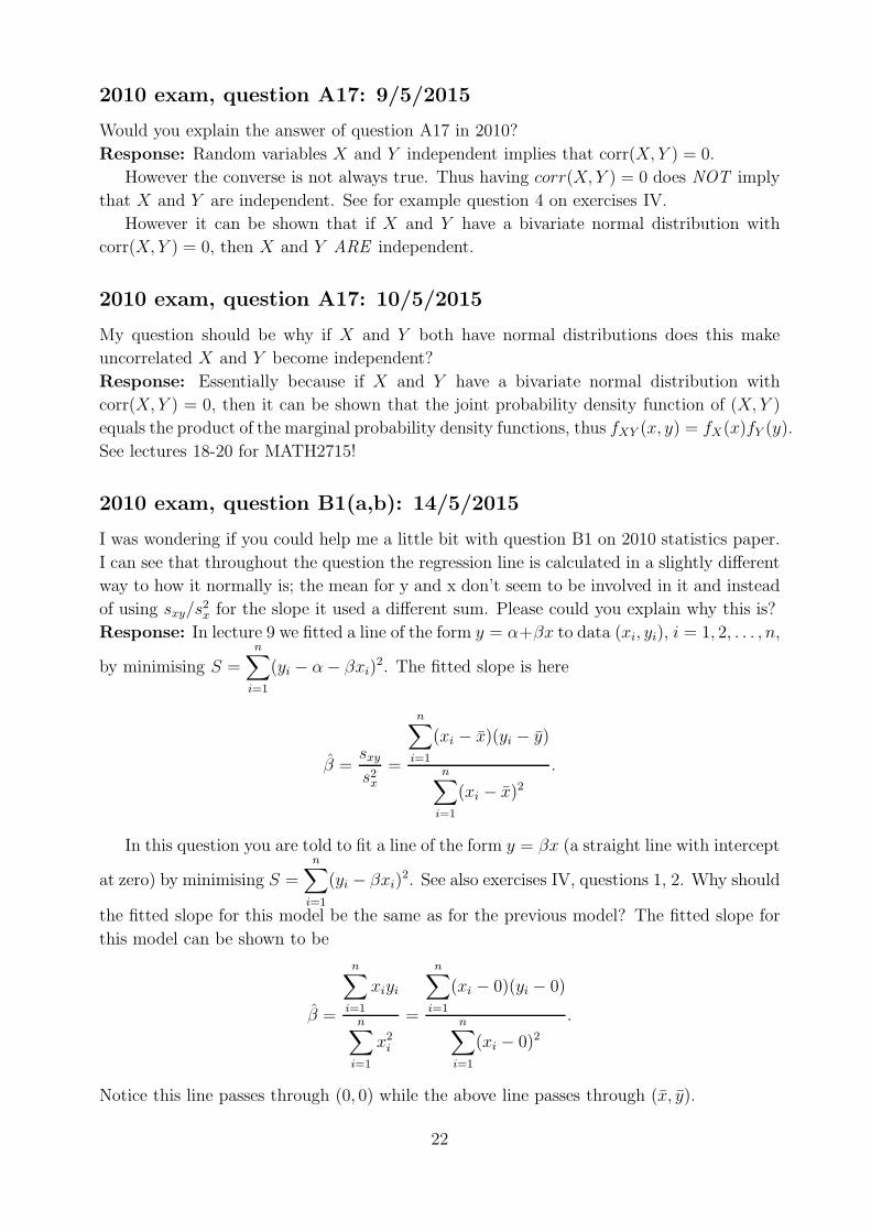
2010 exam, question A17: 9/5/2015
Would you explain the answer of question A17 in 2010?
Response: Random variables X and Y independent implies that corr(X, Y ) = 0.
However the converse is not always true. Thus having corr(X, Y ) = 0 does NOT imply
that X and Y are independent. See for example question 4 on exercises IV.
However it can be shown that if X and Y have a bivariate normal distribution with
corr(X, Y ) = 0, then X and Y ARE independent.
2010 exam, question A17: 10/5/2015
My question should be why if X and Y both have normal distributions does this make
uncorrelated X and Y become independent?
Response: Essentially because if X and Y have a bivariate normal distribution with
corr(X, Y ) = 0, then it can be shown that the joint probability density function of (X, Y )
equals the product of the marginal probability density functions, thus fXY (x, y) = fX(x)fY (y).
See lectures 18-20 for MATH2715!
2010 exam, question B1(a,b): 14/5/2015
I was wondering if you could help me a little bit with question B1 on 2010 statistics paper.
I can see that throughout the question the regression line is calculated in a slightly different
way to how it normally is; the mean for y and x don’t seem to be involved in it and instead
of using sxy/s2x for the slope it used a different sum. Please could you explain why this is?
Response: In lecture 9 we fitted a line of the form y = α+βx to data (xi, yi), i = 1, 2, . . . , n,
by minimising S =n∑
i=1
(yi − α − βxi)2. The fitted slope is here
β =sxy
s2x
=
n∑
i=1
(xi − x)(yi − y)
n∑
i=1
(xi − x)2
.
In this question you are told to fit a line of the form y = βx (a straight line with intercept
at zero) by minimising S =n∑
i=1
(yi − βxi)2. See also exercises IV, questions 1, 2. Why should
the fitted slope for this model be the same as for the previous model? The fitted slope for
this model can be shown to be
β =
n∑
i=1
xiyi
n∑
i=1
x2i
=
n∑
i=1
(xi − 0)(yi − 0)
n∑
i=1
(xi − 0)2
.
Notice this line passes through (0, 0) while the above line passes through (x, y).
22
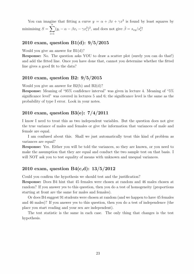
You can imagine that fitting a curve y = α + βx + γx2 is found by least squares by
minimising S =n∑
i=1
(yi − α − βxi − γx2i )
2, and does not give β = sxy/s2x!
2010 exam, question B1(d): 9/5/2015
Would you give an answer for B1(d)?
Response: No. The question asks YOU to draw a scatter plot (surely you can do that!)
and add the fitted line. Once you have done that, cannot you determine whether the fitted
line gives a good fit to the data?
2010 exam, question B2: 9/5/2015
Would you give an answer for B2(b) and B2(d)?
Response: Meaning of “95% confidence interval” was given in lecture 4. Meaning of “5%
significance level” was covered in lectures 5 and 6; the significance level is the same as the
probability of type I error. Look in your notes.
2010 exam, question B3(e): 7/4/2011
I know I need to treat this as two independent variables. But the question does not give
the true variance of males and females or give the information that variances of male and
female are equal.
I am confused about this. Shall we just automatically treat this kind of problem as
variances are equal?
Response: Yes. Either you will be told the variances, so they are known, or you need to
make the assumption that they are equal and conduct the two sample test on that basis. I
will NOT ask you to test equality of means with unknown and unequal variances.
2010 exam, question B4(c,d): 13/5/2012
Could you confirm the hypothesis we should test and the justification?
Response: Does B4 hint that 45 females were chosen at random and 46 males chosen at
random? If you answer yes to this question, then you do a test of homogeneity (proportions
starting at front are the same for males and females).
Or does B4 suggest 91 students were chosen at random (and we happen to have 45 females
and 46 males)? If you answer yes to this question, then you do a test of independence (the
place you start reading and your sex are independent).
The test statistic is the same in each case. The only thing that changes is the test
hypothesis.
23
2009 Examination paper
2009 exam, question A8: 23/4/2011
This asks for the variance of X − 2Y . How do we know whether to include the covariance
term?
Response: Always Var[aX + bY ] = a2Var[X] + b2Var[Y ] + 2ab cov(X, Y ).
You can ignore the covariance term if you know corr(X, Y ) = 0. The question may tell
you that X and Y are uncorrelated so you know corr(X, Y ) = 0, or the question may tell
you that X and Y are independent so you again know that corr(X, Y ) = 0. In this question,
of course, corr(X, Y ) 6= 0!
2009 exam, question A9: 12/4/2011
Could you help me with this question from the 2009 exam paper.
Response: You are told that Var[X] = Var[Y ] = 3 and Var[X + Y ] = 8. Since
Var[aX + bY ] = a2Var[X] + 2ab cov(X, Y ) + b2Var[Y ],
on substituting a = b = 1 you can deduce the value of cov(X, Y ).
2009 exam, question A13: 28/4/2011
Please can you help me with this question.
Response: You are given the values of n, x and s2. You are asked whether the sample
mean is significantly different from zero.
You are being asked to test the hypothesis H0: µ = 0 vs. H1: µ 6= 0 with unknown
variance. See lecture 5.
2009 exam, question A14: 28/4/2011
In A14 values xi and yi, i = 1, 2, . . . , n, lie on a horizontal line y = c where c is a constant.
What does the sample covariance sXY equal? Please can you help me with this question.
Response: You are given observational pairs (x1, y1 = c), (x2, y2 = c), . . . , (xn, yn = c).
What does y equal? Now determine sXY using the formula
sXY =1
n − 1
n∑
i=1
(xi − x)(yi − y).
2009 exam, question A19: 13/5/2012
Question A19 is asking about a confidence interval. I dont know how to do this without a
variance, so I’m not sure what to do!
Response: You are given a proportion p. Here p = 21/161. Recall lecture 17 where an
approximate 95% confidence interval for p was derived. Recall that
p ≈ N
(
π,π(1 − π)
n
)
.
24
Thus tests on π and confidence intervals for π can be based on the fact that
p − π√
π(1 − π)
n
≈ N(0, 1).
Approximate tests and confidence intervals can be obtained using the approximation
p − π√
p(1 − p)
n
≈ N(0, 1).
Notice how the variance is now “known”. The required approximate 95% confidence interval
is thus
p ± 1.96
√
p(1 − p)
n.
2009 exam, question A20: 21/5/2014
What would extremely small values of χ2obs suggest about the experimental data?
Response: We usually do a one-sided χ2-test, checking to see if the observed frequencies
are too different from the expected frequencies. But if the observed and expected frequencies
are too similar, then χ2obs is very small. This is unlikely to be true if the null hypothesis
H0 is true. One explanation is that the observed data were made up by the experimenter –
someone cheated!
2009 exam, question B1(b): 23/5/2010
The question asks me to calculate expected frequencies using the normal distribution and I
can’t figure out how to do this.
Response: Recall lecture 19.
You have already found that x = 71.50′′ and s2 = 7.364. If X represents the height of a
male student, then we can suppose that X ∼ N(µ = 71.5, σ2 = 7.364). Then the expected
probability a male student lies in the “69 to 71” class is, remembering the class boundaries,
pr{68.5 < X ≤ 71.5} = pr
{
68.5 − µ
σ< Z ≤ 71.5 − µ
σ
}
= pr{−1.106 < Z ≤ 0}= pr{Z ≤ 0} − pr{Z ≤ −1.106} = 0.5000 − 0.1345 = 0.3655.
The expected frequency in the “69 to 71” class is thus 100 × 0.3655 = 36.55.
Similarly for the next class. For the “75 to 77” class, make this class open-ended so the
probability a male student lies in this class is pr{X > 74.5}. By doing this we ensure that
the sum of the class probabilities adds to one.
25
2009 exam, question B3(b): 16/5/2015
For question B3 on the 2009 paper, is it asking for another matched pairs test to also be
computed for part (b), before going onto conclude that a matched pairs test is unsuitable
for this data set?
Response: For (b) clearly a matched pairs test is unsuitable. (The data values cannot be
paired – the cuckoos are not laying eggs in both types of test.) It therefore makes no sense
to test the data for differences using a matched pair test if you realise that a matched pair
test is unsuitable. So use a matched pair test in part (a) and a two independent samples
test in part (b).
2009 exam, questions B4(b,c,d): 17/5/2015
Can you please help me with 2009 MATH1725 B4 b,c,d.
Response: If you roll a fair die n times, then the distribution of the number X1 of ones will
follow a Bin(n, π = 1
6) distribution. (Think of tossing a fair coin n times with probability
of heads π.)
If X1 ∼ Bin(n, π), then E[X1] = nπ and Var[X1] = nπ(1 − π).
Y = X1 + X2 is the number of ones or twos observed. Clearly Y ∼ Bin(n, π = 1
3); you
have again n Bernoulli trials (rolls of the die) and a one or a two occurs with probability 1
3.
Thus Var[Y ] = Var[X1 + X2] = n × 1
3× (1 − 1
3) = 2
9n. But you also know that
Var[X1 + X2] = Var[X1] + 2cov(X1, X2) + Var[X2].
You can thus deduce the value of cov(X1, X2) and hence corr(X1, X2).
26
Recommended