Agronomy Research 12(1), 41–58, 2014
Mathematical model of vibration digging up of root
crops from soil
V. Bulgakov1,*
, V. Adamchuk2, G. Kaletnik
3, M. Arak
4 and J. Olt
4
1National University of Bioresources and Nature Management of Ukraine,
15 Heroiv Oborony St., 03041 Kyiv, Ukraine; *Correspondence: [email protected] 2National Scientific Centre ‘Institute for Agricultural Engineering and Electrification’ National Academy of Agrarian Sciences of Ukraine (NAASU), 11 Vokzalna St.,
Glevakha-1, Vasylkiv District, Kyiv Region, 08630, Ukraine 3Vinnitsa National Agrarian University, 3 Soniachna Str., 21008 Vinnytsia, Ukraine
4Institute of Technology, Estonian University of Life Sciences, Kreutzwaldi 56,
EE51014 Tartu, Estonia
Abstract. A new theory of vibrational digging up of root crops from the soil has been
developed. The Hamilton-Ostrogradski variational principle is used, on the basis of which we
have received the differential equation of longitudinal oscillations of the root in the soil with an
infinite number of degrees of freedom. Solution of the given equation provided the possibility
to determine the main parameters of the tools that are used in modern beet harvesters.
Key words: root crop, digging tool, vibrational digging up, variational principle, differential
equation, constructive parameters.
INTRODUCTION
The reason for large-scale use of vibrational digging tools in root harvesters of the
modern technical level is their significantly lower draught level, actual ability to dig up
beetroots from the soil without damage and losses. Oscillations of the digging tool
create conditions, under which the soil that adheres to roots is intensely beaten down
when they are dug up, which facilitates high level of qualitative indicators. That’s why development of new constructions of vibrational digging tools, as well as research of
their operation for the purpose of determination of the optimal constructive and
kinematic parameters is a current task of the branch of mechanisation of sugar beet
growing (Sarec et al., 2009; Lammers, 2011).
Statement of the problem. Analytical research of the process of interaction
between working elements of the vibration digging tool with the root, that allows to
obtain kinematic, constructive and technological parameters, and gives the opportunity
to determine their optimal value.
MATERIAL AND METHODS
Fundamental theoretical and experimental research of the vibrational digging up
of the root crops of sugar beet was published in the paper (Babakov, 1968), in which
the root is modelled as a body having elastic properties, and it is presented as a rod
with variable cross section with one attached end. Transverse oscillations of the root
analysed in the given paper are described using the differential equation, in particular
derivatives of fourth order. The technological process of digging up of the root from
the soil with vibrational application of forces is not actually analysed here; instead it is
stated that using the additionally prepared equations of kinetostatics the conditions are
found for its digging up from the soil under the action of the disturbing force applied in
the cross vertical plane. It is stated in the given paper that this particular direction of
oscillations will be the best way to foster high quality digging up of the root crops from
the soil.
Paper (Vasilenko et al., 1970) presents the theory of the digging tool of a regular
digging share type, and states the conditions for digging up of the root from the soil
with translational motion of the digger, taking the condition of avoiding damage to the
root into account. The given paper demonstrates how the expression is obtained for
determination of the allowed velocity of translational motion of the digging tool with
its pre-set constructive parameters. In the given case the process of digging up of the
root from the soil is performed under the action of forces that emerge on the working
surfaces of the digging shares as a result of the transitional motion of the digging tool
along the rows of the roots.
The developed theory of own and forced oscillations of the body of the root
(Pogorely et al., 1983) is necessary for assessment of the action of the given
oscillations on the process of destruction of connections of the root with the soil.
However, the given methods are not sufficient for performance of full analysis of
the actual process of digging-up of the root from the soil.
Goal of the research. To develop a calculation and mathematical model and to
analytically analyse the root – tool system in order to study the process of oscillations
of the root during its vibrational digging-up from the soil.
RESULTS OF THE RESEARCH
The case where oscillatory motions of the vibration digging-up tool are applied to
the beetroot in longitudinal vertical area will now be analytically analysed. It will be
assumed that the root that is located in the soil is a complex solid elastic system with
an infinite number of degrees of freedom, also modelled as the rod with variable cross
section with the attached low end.
At the same time, since the Lagrange equation of the second kind in generalised
coordinates serves as theoretical basis for most research of oscillations of holonomic
systems with a finite number of degrees of freedom, for the purpose of performance of
oscillations of holonomic systems with an infinite number of degrees of freedom the so
called Hamilton-Ostrogradski principle of stationary action is used (Babakov, 1968).
In the theory of longitudinal, torsional and transverse oscillations of straight rods
the Hamilton-Ostrogradski functionals are applied, which in the most generalised form
look as follows:

tdxdx
y
xt
y
t
y
x
y
t
yyxtLS
t
t
h
ò ò ÷÷ø
öççè
æ
¶¶
¶¶¶
¶¶
¶¶
¶¶
=2
1 0
2
22
2
2
,,,,,,,
(1)
where: ПTL -= is the Lagrange function; T is kinetic energy of the system; П is
the potential energy of the system.
It will be assumed that the root that is located in the soil to be the rod with
variable cross section along its length with one end attached (Fig. 1). The Hamilton-
Ostrogradski principle will now be applied for research of longitudinal oscillations of
the root that occur under the action of the vertical disturbing force that changes
according to the harmonic law of the following type (Bulgakov et al., 2005):
tHQзб
wsin.=
, (2)
where: H is the amplitude of forced oscillations; w is the frequency of forced
oscillations.
As we can see from the scheme (Fig. 1), the root having a cone-like body (the top
angle of which equals g2 , and the top part of which is located above the level of the
surface of the soil), is modelled as the rod with variable cross section with the attached
low end (point O). In the centre of gravity, designated as point C , the force G is
applied – the weight force of the root. h is its total length. Through the axis of
symmetry of the root the vertical axis x is drawn, the beginning of which matches the
point O. Connection of the root with the soil is determined by the general reaction of
the soil xR , which is located along the axis x .
Figure 1. Scheme of the forces having an action on the root at the time of gripping by the
vibration digging tool.
The disturbing force .збQ stated above is simultaneously applied to the root from
two digging-up plough shares from its two sides, and that’s why it is presented in the scheme by two components
1.збQ and 2.збQ . The given forces are applied on the
distance 1x from the origin of coordinates (point O), and they are the source of
oscillations of the root in longitudinal vertical area, that destroy connection of the root
with the soil and form conditions for digging up of the latter from the soil. The
functional S of Hamilton-Ostrogradski for the analysed vibrational process will now
be made. For this purpose the necessary symbols will be applied:
)(xF is the area of cross section of the root at some point located at the distance
x from the low end m2; E is the Young's modulus for material of the root N m
-2;
( )txy , is the longitudinal dislocation of some cross section of the root at the time point
t , m; ),( txQ is the intensity of longitudinal external load directed along the axis of
the root N m-1
; ( )xm is the mass per length of the root kg m-1
.
Then kinetic energy of the oscillatory motion of the root will be:
( )ò ÷÷ø
öççè
æ
¶¶
=h
o
xdt
yxT
2
2
1m
(3)
Potential energy of the elastic deformation is designated as follows:
( )ò ÷÷ø
öççè
æ
¶¶
×=h
o
xdx
yxFEП
2
12
1
(4)
Potential stretching energy of the longitudinal load ( )txQ , will look as follows:
( )ò=h
o
xdytxQП ,2
12
(5)
The Lagrange function L will be made.
Since
21 ППTL +-= , (6)
then, taking the expressions (3), (4) and (5) into consideration, we get:
( ) ( ) ( ) .,2
122
xdytxQx
yxFE
t
yxL
h
o
òúúû
ù
êêë
é+÷÷
ø
öççè
æ
¶¶
×-÷÷ø
öççè
æ
¶¶
= m (7)
By inserting the expression (7) into the expression (1), we will have:
( ) ( ) ( ) .,2
1 2
1
22
tdxdytxQx
yxFE
t
yxS
t
t
h
o
ò òúúû
ù
êêë
é+÷÷
ø
öççè
æ
¶¶
×-÷÷ø
öççè
æ
¶¶
= m (8)
Further, expressions of all values that are included in the functional (8) will be
found. Since the root has the shape of a cone, we find that its area of cross section F(x)
at the point that is located at an arbitrary distance x from the point O, will be:
( ) gp 22 tanxxF = . (9)
It is obvious that the mass per length of the root can be determined using the
following expression:
( ) ( )xFx ×= rm ,
or, given the (9),
( ) gprm 22 tanхx ×= , (10)
where r is the density of the root in kg m-3
.
Since the value Q(x,t), included in the functional (8), is the intensity of distributed
load, that is measured in N m-1
, then in each specific case the disturbing force must
correspond to dimension of the intensity of the load. By using the so called impulse
function of the first order σ1(x) (Babakov, 1968) it is possible to determine the intensity
of the distributed load, and to include into the composition of the load divided along
the length the concentrated forces and moments of forces.
Respectively, if ( )tQзб.
is the concentrated disturbing force applied to point 1x
and measured in Newtons, then the function:
( ) ( ) ( )11.. , xxtQtxQзбзб
-×= s (11)
has the dimension in N m-1
and expresses intensity of the concentrated load in the
point 1x .
The function ( )11 xx -s equals zero for all x , except for 1xx = , where it is
transformed into infinity.
Let the disturbing force acting according to the law
( ) tHtQзб
wsin. = , (12)
be applied to the root at the distance 1x from the starting point (point O in Fig. 1).
Then, according to (11) we can write:
( ) ( )11. sin, xxtHtxQзб
-×= sw . (13)
Since the root is connected with the soil, which is an elastic environment,
application of the disturbing force of type (12) to the root leads to emergence of the
force of resistance of the soil to movement of the root due to its oscillations. This force
also has an action on the process of own oscillations of the root in the soil, especially at
the beginning of the oscillations process, until connections of the root with the soil are
destroyed.
It is obvious that the force of resistance of the soil (for the entire body of the root)
is the distributed load along the area of contact of the root with the soil, and that’s why we must determine its intensity as the force of resistance of the soil to movement of a
length unit of the root.
Let c be the coefficient of the elastic deformation of the soil applied to the area of
the contact measured in N m-2
. It will now be assumed that the soil surrounding the
root, under the action of the disturbing force Hsinωt, performs forced oscillations
according to the same harmonic law with the amplitude that is determined by elastic
properties of the soil. Then the intensity P(x, t) in N m-1
of resistance of the soil to
movement of the root in point x will be:
( ) ,sintan2, txctxP wgp ××= (14)
Respectively, we will have the following relation for longitudinal external load:
( ) ( ) ( )txPtxQtxQзб
,,, . -= .
Given the expressions (9), (10), (13) and (14), the Hamilton-Ostrogradski
functional (8) will look as follows:
( )[ ] ( ) .,sintan2sin
tantan2
1
11
2
22
2
0
222
1
tddxtxytxcxxtH
x
yxE
t
yxS
t
t
h
þýü
××--×+
+÷÷ø
öççè
æ
¶¶
×-îíì
÷÷ø
öççè
æ
¶¶
×= ò ò
wgpsw
gpgpr (15)
In order to find natural forms and frequencies of longitudinal oscillations of the
root in the soil, the Ritz method can be applied (Babakov, 1968). According to the
given method we will need to find harmonic longitudinal oscillations of the root as
follows:
( ) ( ) ( )aj += tpxtxy sin, , (16)
where )(xj is the natural form of primary oscillations, i.e. the function that
determines continuous population of amplitude longitudinal deviations of cross section
of the root from their equilibrium positions, and p is the natural frequency of primary
oscillations.
Since natural forms and natural frequencies are related to free oscillations of the
system, in the functional (15) we must highlight the part that specifically describes free
oscillations of the system. Obviously the functional will look as follows:
dtdxx
yxE
t
yxS
t
t
h
o
ò òúúû
ù
êêë
é÷÷ø
öççè
æ
¶¶
-÷÷ø
öççè
æ
¶¶
=2
1
2
22
2
22
1 tantan2
1gpgrp (17)
The expression (16) will now be inserted into the functional (17), and we will get:
( ) ( )
( )[ ] .sintan
costan2
1
2222
22
0
222
1
2
1
tdxdtpxxE
tppxxS
t
t
h
þýü÷ø
öçè
æ +¢×-
-+××îíì
×××= ò ò
ajgp
ajgpr
(18)
The expression (18) will be integrated over t within the limits of one period
,2
pT
p= and we will have:
( ) ( )[ ] .tantan2
222
0
2222
2 dxxxEpxxp
S
h
þýü¢×
îíì
-×××= ò jgpjgprp
(19)
The basis of the Ritz method is reduction of the variational problem to the
problem of search of extremum of function of any independent variables.
According to the Ritz method the value of the functional (19) is analysed on
population of linear combinations of functions, i.e. expressions looking as follows:
( ) ( )å=
×=n
i
ii xx1
yay , (20)
where: αi are the parameters, variations of which enable us to obtain the required class
of allowed functions; )(xiy are the basis functions that are specifically chosen and are
known functions, that correspond to geometrical boundary conditions of the problem.
Respectively, we insert the expression (20) into the expression (19), and get:
( )
( ) .tan
tan2
2
1
22
0
2
2
1
22
2
xdxxE
pxxp
S
n
i
ii
h n
i
ii
ïþ
ïý
ü
úú
û
ù
êê
ë
é ¢÷ø
öçè
æ×-
ïî
ïíì
-úû
ùêë
é×=
å
ò å
=
=
yagp
yagprp
(21)
After respective transformations the functional (21) will look as follows:
( ) ( )
( ) ( ) .tan
tan2
1,
22
0 1,
222
2
dxxxxE
xxpxp
S
n
ki
kiki
h n
ki
kiki
úû
ù¢¢-
êë
é-=
å
ò å
=
=
aayygp
aayygrpp
(22)
The following symbols will now be entered:
( ) ( )
( ) ( ) ,tan
,tan
0
22
0
22
ikk
h
i
ikk
h
i
UxdxxxE
Txdxxx
=¢×¢××
=××××
ò
ò
yygp
yygpr
(23)
( )nki ,...,2,1, = .
By inserting (23) into (22), we will get a functional as a function from parameters
:,,, 21 naaa K
( ) .22
...,,,1,1,
2
212 ki
n
ki
ik
n
ki
kiikn Up
Tpp
S aap
aap
aaa åå==
-= (24)
The extremum analysis of the functional (24) will now performed. For this
purpose we will differentiate the expression (24) with respect to parameters αi,
),,2,1( ni K= and equate the obtained particular derivatives to zero. As a result of
that we will get a set of linear homogeneous equations with respect to the unknowns
,,,, 21 naaa K from which, in turn, we can find the Ritz frequencies equation for
longitudinal oscillations of the root attached in the soil:
0
...
.......................................................................
...
...
2
2
2
21
2
1
2
2
222
2
2221
2
21
1
2
112
2
1211
2
11
=
---
---
---
nnnnnnnn
nn
nn
TpUTpUTpU
TpUTpUTpU
TpUTpUTpU
(25)
It is known, that with 4>n the given equation cannot be solved in radicals,
that’s why it is necessary to apply numerical methods using a PC. However, in reality, as a rule, only the lower frequencies are determined, most
often the first and the second ones, which have the most significant action on the
technological process that is being analysed.
Therefore, the first and the second frequencies of natural oscillations of the root
will now be determined.
For the purpose of determination of the first and the second frequencies the
equation (25) will look as follows:
0
22
2
2221
2
21
12
2
1211
2
11 =--
--
TpUTpU
TpUTpU (26)
As a result of the solution of the given equation we will obtain expressions for
finding the value of the first (primary) frequency:
rE
hp
662422.01 = , (27)
and the second frequency:
rE
hp
931592.272 = . (28)
Now the calculation will be performed of the values of the first and the second
frequencies for the beetroot having the following parameters (Pogorely et al., 1983)
250=h mm; 6104.18 ×=E N m-2
; 300,1=r kg m-3
. As a result of the calculations we
get:
315300,1
104.18
10250
662422.0 6
31 =×
×=
-p s
-1,
292,13130
104.18
10250
931592.27 6
32 =×
×=
-p s
-1.
Next, the analysis of the forced oscillations of the root will be discussed. The
exclusively forced oscillations will happen according to the following law:
( ) ( ) txtxy wj sin, = , (29)
where j(x) is the form of the forced oscillations.
In order to determine the form of the forced oscillations of the root the expression
(29) will now be entered into the functional (15), and we will get the following
functional:
( ){ ( )[ ]
( )[ ] ( ) .sintan2
sintancostan2
1
2
1
22222
0
2222
3
2
1
tdxdtxcxxxH
txxEtxxS
t
t
h
þýü--+
+¢-= ò ò
wjgps
wjgpwjgwpr (30)
By integrating the expression (30) over t within the limits of one period
,2
wp
=T we will get:
( ) ( )[ ]
( ) ( ) ( ) .tan2
tantan2
11
222222
0
2
4
xdxcxxxxH
xxExxS
h
þýü--+
+¢-îíì
= ò
gjpjs
jgpwgjprwp
(31)
According to the Ritz method let’s analysis will now performed of the value of the functional (31) with respect to population of linear combinations of the following
type:
( ) ( )xx yaj = (32)
where: a is the parameter, variations of which let us obtain the class of the allowed
functions; ( )xy is the basis function.
The expression (32) will now be inserted into the functional (31), and we will
obtain:
( ) ( )[ ]
( ) ( ) ( ) .tan2
tantan2
11
22222222
0
2
4
xdxxcxxxH
xxExxS
h
þýü--+
+¢-îíì
= ò
gaypays
jgapwygaprwp
(33)
The following symbols will now be inserted:
( )ò =××h
Txdxx0
222 tan ygpr , (34)
( )[ ] UxdxxE
h
=¢××ò0
222 tan ygp , (35)
( ) ( )[ ( )] .tan20
11 LxdxxcxxxH
h
=-×-ò gypys (36)
The expressions (34), (35), (36) will now be inserted into (33), and we will have:
( ) ( )aaawwp
a LUTS +-= 222
42
(37)
So, in the population of functions, (32) the functional (33) is transformed into the
function of the independent variable ,a looking as (37).
The necessary condition of the stationary functional (37) (i.e. existence of the
extremum) is that its first variation equals zero:
04 =׶
adaS
(38)
from which we receive the following equation:
022 2 =+- LUT aaw (39)
from which we find the required value of the parameter a . It will be:
( )TU
L22 w
a-
= (40)
The form of the forced longitudinal oscillations of the rod with the constant cross
section with one end firmly attached, emerging under the action of the longitudinal
harmonic force of frequency ,w applied at the point 1xx = will now be assumed as the
basis function )(ty .
According to Babakov (1968) the form of the forced oscillations of the given rod
looks as follows:
( ) xaDx sin1=y with 1xx £ (41)
( ) ( )xhaDx -= cos2y with 1xx > , (42)
where, ( )
ha
xha
FEaD
cos
cos1 11
-×-= (43)
ha
xa
FEaD
cos
sin1 12 ×-= (44)
FEa
mw= (45)
m is the mass per length of the rod; F is the area of the longitudinal section of the
rod; E is the Young’s module for material of the rod; h is the length of the rod; w is
the frequency of the forced oscillations of the rod.
Having calculated the parameters of T, U and L according to the expressions (34),
(35) and (36), we obtain the required value of the parameter a according to the
expression (40), in case of which the functional (33) will have a stationary value.
Taking into consideration the expressions (32), (41) and (42), we get expression
for the form of the forced oscillations of the root attached in the soil. They look as
follows:
( ) xaDx sin1×=aj , with
,1xx £ ( ) ( )xhaDx -×= cos2aj , with 1xx > . (46)
Having inserted the expressions (46) into (29), we get the final law of the forced
oscillations of the root attached in the soil. If we take into consideration the action of
the disturbing force ,sin tH w the given law will look as follows:
( ) taxDtxy wa sinsin, 1 ×= , with 1xx £ ,
( ) ( ) txhaDtxy wa sincos, 2 ×-= , with 1xx > . (47)
Based on the results of the theoretical research of the forced oscillations of the
beetroot attached in the soil we will perform specific calculations of the amplitude of
the given oscillations.
The length of the root h , its cone angle g , Young’s module E for the body of
the root, density r of the root, coefficient of elastic deformation of the soil c will be
assumed to be equal, according to Pogorely et al. (1983): h = 250ˑ10-3 m; γ = 14°;
E = 18.4ˑ106 N m-2; ρ = 1,300 kg m
-3; c = 1ˑ10-5
N m-2
.
The amplitude H of the disturbing force will be chosen within the limits
100...600 N. We will assume the frequency ω of the disturbing force, according to
(Vasilenko et al., 1970), to equal w = 20 Hz.
The calculation is performed using the Mathcad program in order to determine the
relations between the amplitude of the forced longitudinal oscillations of the body of
the root and changes of the disturbing force within the range 100...600 N for different
cross sections of the root.
The result of the given calculation is the graph shown in Fig. 2.
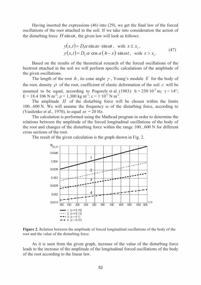
Figure 2. Relation between the amplitude of forced longitudinal oscillations of the body of the
root and the value of the disturbing force.
As it is seen from the given graph, increase of the value of the disturbing force
leads to the increase of the amplitude of the longitudinal forced oscillations of the body
of the root according to the linear law.
It should also be noted, that with increase of the distance of the area of cross
section of the root from the origin of coordinates O the amplitude is also increased. For
example, with x = 0.07 m the amplitude is within the limits of 1.7…2.3 mm with
x = 0.1 m – within the limits of 2.3…3.5 mm, with x = 0.12 m – within the limits of
2.8…3.9 mm, with x = 0.15 m (the point of gripping) – within the limits 3.2…4.8 mm.
Further, analysis will be presented of the calculation performed on a PC of the
amplitude of longitudinal oscillations of the body of the root attached in the soil from
the coefficient c of the elastic deformation of the soil surrounding the root, and the
distance of the cross section of the root from the conditional point of its attachment for
the frequency of the disturbing force 10=v Hz and 20=v Hz.
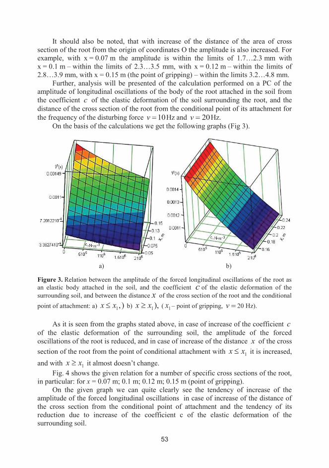
On the basis of the calculations we get the following graphs (Fig 3).
a) b)
Figure 3. Relation between the amplitude of the forced longitudinal oscillations of the root as
an elastic body attached in the soil, and the coefficient c of the elastic deformation of the
surrounding soil, and between the distance x of the cross section of the root and the conditional
point of attachment: a) ),1xx £ b) ),1xx ³ ( 1x – point of gripping, =v 20 Hz).
As it is seen from the graphs stated above, in case of increase of the coefficient c
of the elastic deformation of the surrounding soil, the amplitude of the forced
oscillations of the root is reduced, and in case of increase of the distance x of the cross
section of the root from the point of conditional attachment with 1xx £ it is increased,
and with 1xx ³ it almost doesn’t change.
Fig. 4 shows the given relation for a number of specific cross sections of the root,
in particular: for x = 0.07 m; 0.1 m; 0.12 m; 0.15 m (point of gripping).
On the given graph we can quite clearly see the tendency of increase of the
amplitude of the forced longitudinal oscillations in case of increase of the distance of
the cross section from the conditional point of attachment and the tendency of its
reduction due to increase of the coefficient c of the elastic deformation of the
surrounding soil.
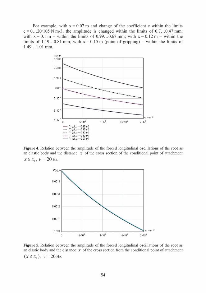
For example, with x = 0.07 m and change of the coefficient c within the limits
c = 0…20ˑ105 N m-3, the amplitude is changed within the limits of 0.7…0.47 mm;
with x = 0.1 m – within the limits of 0.99…0.67 mm; with x = 0.12 m – within the
limits of 1.19…0.81 mm; with x = 0.15 m (point of gripping) – within the limits of
1.49…1.01 mm.
Figure 4. Relation between the amplitude of the forced longitudinal oscillations of the root as
an elastic body and the distance x of the cross section of the conditional point of attachment
1xx £ , 20=n Hz.
Figure 5. Relation between the amplitude of the forced longitudinal oscillations of the root as
an elastic body and the distance x of the cross section from the conditional point of attachment
),( 1xx ³ 20=v Hz.
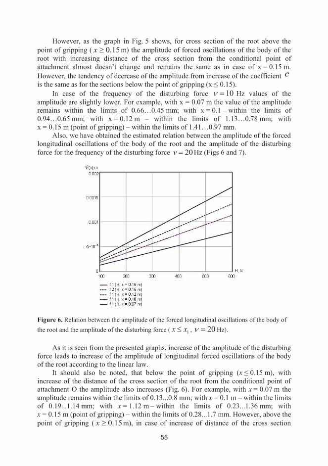
However, as the graph in Fig. 5 shows, for cross section of the root above the
point of gripping ( 15.0³x m) the amplitude of forced oscillations of the body of the
root with increasing distance of the cross section from the conditional point of
attachment almost doesn’t change and remains the same as in case of x = 0.15 m.
However, the tendency of decrease of the amplitude from increase of the coefficient c
is the same as for the sections below the point of gripping (x ≤ 0.15).
In case of the frequency of the disturbing force 10=n Hz values of the
amplitude are slightly lower. For example, with x = 0.07 m the value of the amplitude
remains within the limits of 0.66…0.45 mm; with x = 0.1 – within the limits of
0.94…0.65 mm; with x = 0.12 m – within the limits of 1.13…0.78 mm; with
x = 0.15 m (point of gripping) – within the limits of 1.41…0.97 mm.
Also, we have obtained the estimated relation between the amplitude of the forced
longitudinal oscillations of the body of the root and the amplitude of the disturbing
force for the frequency of the disturbing force 20=v Hz (Figs 6 and 7).
Figure 6. Relation between the amplitude of the forced longitudinal oscillations of the body of
the root and the amplitude of the disturbing force ( 1xx £ , 20=n Hz).
As it is seen from the presented graphs, increase of the amplitude of the disturbing
force leads to increase of the amplitude of longitudinal forced oscillations of the body
of the root according to the linear law.
It should also be noted, that below the point of gripping (x ≤ 0.15 m), with
increase of the distance of the cross section of the root from the conditional point of
attachment O the amplitude also increases (Fig. 6). For example, with x = 0.07 m the
amplitude remains within the limits of 0.13...0.8 mm; with x = 0.1 m – within the limits
of 0.19...1.14 mm; with x = 1.12 m – within the limits of 0.23...1.36 mm; with
x = 0.15 m (point of gripping) – within the limits of 0.28...1.7 mm. However, above the
point of gripping ( 15.0³x m), in case of increase of distance of the cross section
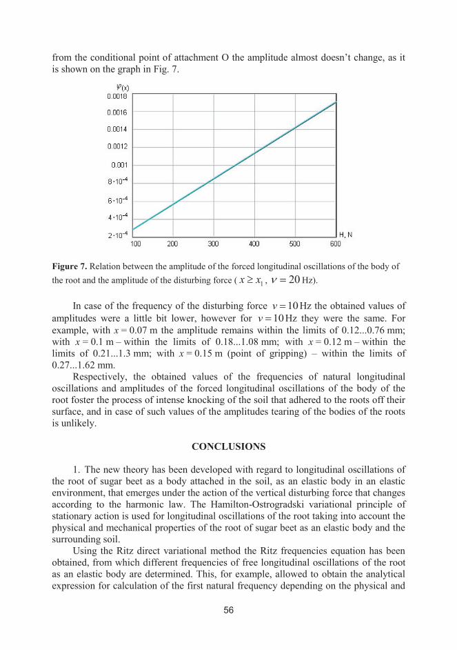
from the conditional point of attachment O the amplitude almost doesn’t change, as it
is shown on the graph in Fig. 7.
Figure 7. Relation between the amplitude of the forced longitudinal oscillations of the body of
the root and the amplitude of the disturbing force ( 1xx ³ , 20=n Hz).
In case of the frequency of the disturbing force 10=v Hz the obtained values of
amplitudes were a little bit lower, however for 10=v Hz they were the same. For
example, with x = 0.07 m the amplitude remains within the limits of 0.12...0.76 mm;
with x = 0.1 m – within the limits of 0.18...1.08 mm; with x = 0.12 m – within the
limits of 0.21...1.3 mm; with x = 0.15 m (point of gripping) – within the limits of
0.27...1.62 mm.
Respectively, the obtained values of the frequencies of natural longitudinal
oscillations and amplitudes of the forced longitudinal oscillations of the body of the
root foster the process of intense knocking of the soil that adhered to the roots off their
surface, and in case of such values of the amplitudes tearing of the bodies of the roots
is unlikely.
CONCLUSIONS
1. The new theory has been developed with regard to longitudinal oscillations of
the root of sugar beet as a body attached in the soil, as an elastic body in an elastic
environment, that emerges under the action of the vertical disturbing force that changes
according to the harmonic law. The Hamilton-Ostrogradski variational principle of
stationary action is used for longitudinal oscillations of the root taking into account the
physical and mechanical properties of the root of sugar beet as an elastic body and the
surrounding soil.
Using the Ritz direct variational method the Ritz frequencies equation has been
obtained, from which different frequencies of free longitudinal oscillations of the root
as an elastic body are determined. This, for example, allowed to obtain the analytical
expression for calculation of the first natural frequency depending on the physical and
mechanical properties of the root and elasticity of the soil surrounding it, which plays
the main role in destruction of the tights of the root with the soil. According to the
calculations performed, when the coefficient c of the elastic deformation of the soil is
changed, the first frequency of natural oscillations of the body of the root is
monotonously increased within the limits of 76.4…93.4 Hz, which sufficiently
precisely corresponds to the experimental data stated in (Pogorely et al., 1983;
Pogorely & Tatyanko, 2004). At the same time the second frequency is changed within
the limits of 528…532 Hz, i.e. it has little dependency on the coefficient c of the elastic
deformation of the soil.
2. The Hamilton-Ostrogradski functional for forced longitudinal oscillations of
the root as an elastic body was constructed, on the basis of which the theory of forced
oscillations of the beetroot in the soil was created. The results of theoretical research of
the forced oscillations of beetroot attached in the soil were the basis for finding of the
algorithm for calculation on a PC of the specified oscillations, in particular, finding of
the law of the forced longitudinal oscillations and amplitude under the condition of
prevention of damage (tearing) of the beetroot depending on the coefficient c of the
elastic deformation of the soil and the amplitude of the disturbing force.
3. It was analytically established that the amplitude of the forced oscillations of
the body of the root decreases in case of increase of the coefficient c of elastic
deformation of the soil, and increases in case of increase of distance of the cross
section of the beetroot from the conditional point of its attachment in the soil. For
example, with x = 0.07 m and the change of the coefficient c within the limits of
c = 0…20ˑ105 N m
-3, the amplitude is measured within the limits of 0.7…0.47 mm;
with x = 0.1 m – within the limits of 0.99…0.67 mm; with x = 0.12 m – within the
limits of 1.19…0.81 mm; with x = 0.15 m (point of gripping) – within the limits of
1.49…1.01 mm.
However, for the cross sections of the root above the point of gripping
(x ≥ 0.15 m) the amplitude of the forced oscillations of the body of the root almost
doesn’t change in case of increase of the distance of the cross section from the
conditional point of attachment and remains the same as in case of x = 0.15 m.
However, the tendency of decrease of the amplitude from increase of the coefficient cis the same as for sections below the point of gripping (x ≤ 0.15 m).
4. The paper also presents the calculations performed of the amplitude of forced
longitudinal oscillations in case of change of the amplitude of the disturbing force
within the limits of 100…600 N. As the calculations demonstrated, the increase of the
amplitude of the disturbing force leads to the increase of the longitudinal forced
oscillations of the body of the beetroot according to the linear law, and increase of the
distance of the area of cross section of the root from the conditional point of its
attachment in the soil also leads to increase of the amplitude.
For example, with x = 0.07 m, the amplitude remains within the limits of
0.13…0.8 mm, with x = 0.1 m – within the limits of 0.19…1.14 mm,
with x = 0.12 m – within the limits of 0.23…1.36 mm, with x = 0.15 m (point of
gripping) – within the limits of 0.28…1.7 mm. However, above the point of gripping in
case of increase of the distance of the cross section from the conditional point of
attachment the amplitude almost does not change.
REFERENCES
Babakov, I.M. 1968. Theory of Oscillations. Nauka, Moscow, 560 pp. (in Russian).
Bulgakov, V., Golovats, I., Špokas, L. & Voitjuk, D. 2005. Theoretical investigation of a root
crop cross oscillations at vibratinal digging up. Research papers of IAg Eng LUA & LU of
Ag. 37(1), 19–35. (in Russian).
Lammers, P.S. 2011. Harvest and loading machines for sugar beet – new trends. International
Sugar Journal 113(1348), 253–256.
Pogorely, L.V., Tatyanko, N.V., & Bray, V.V. 1983. Beet-harvesting machines (designing and
calculation). Under general editorship of Pogorely, L. V. Tehnika, Kyiv, 232 pp.
Pogorely, L.V., & Tatyanko, N.V. 2004. Beet-harvesting machines: History, Construction,
Theory, Prognosis, Feniks, Kyiv, 232 pp. (in Ukrainian).
Sarec, P., Sarec, O., Przybyl, J., & Srb, K. 2009. Comparison of sugar beet harvesters. Listy
cukrovarnicke a reparske 125(7-8), 212–216. (in Czech).
Vasilenko, P.M., Pogorely, L.V., & Brey, V.V. 1970. Vibrational Method of Harvesting Root
Plants. Mechanisation and Electrification of the Socialist Agriculture 2, 9–13
(in Russian).
Recommended