May 2016


MINISTERO DELL’ECONOMIA E DELLE FINANZE III
INDEX
KEY POINTS ....................................................................................................................................... 1
OVERVIEW ............................................................................................................................... 3
I. CYCLICAL CONDITIONS ........................................................................................................ 9
I.1 The italian economy and the international environment .................................................................. 9
I.2 Sensitivity analysis: worsening global conditions and fiscal tightening ......................................... 10
I.3 Deflationary pressures and monetary accommodation .................................................................. 11
I.4 Estimation of output gap and potential growth ............................................................................... 14
II. CYCLICAL CONDITIONS AND CONSISTENCY BETWEEN THE PREVENTIVE ARM
OF THE SGP AND THE DEBT RULE ................................................................................... 27
II.1 Cyclical conditions and the debt rule .............................................................................................. 27
III. STRUCTURAL REFORMS .................................................................................................. 33
III.1 Progress on the Reform Agenda ..................................................................................................... 33
III.2 Structural reforms and impact on GDP, long term gains and short term costs .......................... 40
IV. MEDIUM TERM BUDGETARY POSITION ........................................................................... 45
IV.1 Structural deficit, fiscal consolidation and convergence to the MTO ........................................... 45
IV.2 Italy’s track record on primary balance, developments in primary spending
and quality of public finances ........................................................................................................ 47
V. DEVELOPMENTS IN GOVERNMENT DEBT POSITION ........................................................ 53
V.1 Developments in government debt position ................................................................................... 53
V.2 Impact of QE on debt/GDP ratio ...................................................................................................... 55
V.3 Risks related to the structure of public debt financing .................................................................. 58
V.4 Participation in Euro Area solidarity Programmes, Trade debt arrears and
privatisations ................................................................................................................................... 60
VI. DEBT SUSTAINABILITY ..................................................................................................... 63
VI.1 Medium Term Debt-to-GDP projections ......................................................................................... 63
VI.2 Fiscal sustainability in light of ageing populations ........................................................................ 69
VII. OTHER RELEVANT FACTORS ........................................................................................... 73
VII.1 Private sector debt ......................................................................................................................... 73
VII.2 Costs of immigration and refugee crisis ....................................................................................... 74

IV MINISTERO DELL’ECONOMIA E DELLE FINANZE

MINISTERO DELL’ECONOMIA E DELLE FINANZE 1
KEY POINTS
Italy’s gross public debt-to-GDP ratio virtually stabilized in 2015, reaching 132.7
percent of GDP from 132.5 percent in 2014 despite adverse global economic conditions
and statistical revisions. The government expects the debt ratio to decline to 132.4
percent in 2016 and more sharply in 2017-2019, reaching 123.8 percent in 2019.
Since 2012, thanks to consistent primary surpluses, Italy’s budget deficit has fulfilled
the 3 percent-of-GDP ceiling. It fell from 3.0 percent in 2014 to 2.6 percent in 2015. It
will decline further to 2.3 percent this year and 1.8 percent in 2017. Accelerated
deficit reduction is planned for 2018-2019, leading to a small budget surplus in 2019.
The debt-reduction rule would be broadly satisfied on a forward-looking basis in 2017.
The sharp decline in the debt ratio projected for 2017-2019 is predicated on higher
nominal GDP growth, larger primary surpluses, significant privatization revenues, lower
interest payments and a shrinking gap between deficits and borrowing requirements.
The economic environment is extremely challenging for debt reduction, as global
deflationary pressures have intensified. The inflation rate is negative, and the impact
of the euro exchange rate depreciation on prices will taper off in the next two years.
Worldwide excess capacity is substantial, competitive pressures are growing in all
sectors of the economy, energy prices could remain low for an extended period of time.
Slow nominal GDP growth entails slower progress on public debt reduction. Lower bond
yields take time to reduce overall interest costs, as the financial duration of Italy’s
public debt has risen in recent years reflecting a prudent debt-management approach.
We provide econometric evidence suggesting that despite a substantial accommodation
in Euro area monetary conditions, over the past two years the external economic
environment adversely impacted Italy’s nominal GDP growth and the debt-to-GDP ratio.
It is also shown that tighter fiscal policy compared to the 2016 Stability Program would
worsen the growth performance of the Italian economy and the evolution of the debt-
to-GDP ratio. This argument is particularly relevant at low levels of economic activity,
as fiscal multipliers are larger and fiscal consolidation risks being self-defeating.
The estimation of Italy’s structural budget balance is beset by serious empirical issues.
Potential growth estimated by the Commission is negative. Italy’s negative output gap
was revised down for spurious reasons and is projected to close within two years.
The output gap is underestimated. We propose changes in the production function
methodology that improve the econometric fit and yield a wider output gap. Based on a
more realistic and wider negative output gap estimate, Italy’s fiscal policy in 2016 and
the plan announced for 2017-2019 are compliant with the Stability and Growth Pact.
Italy’s structural reform effort continues at full speed. The effect of recent reforms is
estimated at 2.2 percentage points of GDP by 2020, 3.4 points by 2025 and 8.2 in the
long run. Other relevant factors discussed in this report include Italy’s track record of
fiscal discipline and the budgetary impact of the ongoing large wave of immigration.

2 MINISTERO DELL’ECONOMIA E DELLE FINANZE

MINISTERO DELL’ECONOMIA E DELLE FINANZE 3
OVERVIEW
This note summarizes the relevant factors that the government feels should be taken into account in assessing Italy’s compliance with the debt criterion according to article 126.3 of the European Treaty.
Reducing the public debt-to-GDP ratio is one of the key economic policy goals of the Italian government. However, the pace of fiscal consolidation should be economically and socially sustainable. The fiscal policy strategy should take into account deflation risks and should not cause further lasting damage to Italy’s productive capacity and employment.
1. Deflation risks
Europe is at risk of falling into outright deflation. The Euro area economy expanded in the first quarter of 2016, but the global economic outlook is more challenging than expected until recently. The downturn in Emerging Markets is deeper. Falling energy and commodity prices have eroded the buying capacity of Europe’s hitherto most dynamic exports markets, while China’s excess capacity puts downward pressure on prices of manufactured goods.
In Europe, weak demand is causing deflationary pressures even in the service sector. The European Commission’s Spring 2016 Economic Forecast acknowledges the condition of near-deflation Europe is facing, as it projects an average inflation rate for the Euro area of 0.2 percent this year, following a reading of zero in 2015.
The Commission’s Spring Forecast calls for a rise in the headline inflation to 1.4 percent in 2017. The latest Eurostat data, however, suggest that the Euro area inflation rate fell to -0.2 percent in April, with core inflation down to 0.7 percent. The rise in headline inflation predicted by the Commission for 2017 is predicated on higher energy prices and on a narrowing of the output gap, which should lead to a return of domestic inflation pressures. This scenario is similar to the ones of other official organization and member states. However, expectations of a resurfacing of inflation pressures have so far been consistently disappointed, and forecasts have been marked down as a result. At any rate, the Commission’s inflation forecast is based on three fundamental judgements that are either debatable or subject to considerable risks.
The first is the estimated level of the Euro area output gap and the speed at which it is expected to narrow in the next two years. In our view, the Commission’s output gap projections underestimate the degree of slack in the Euro area economy, especially for member countries that have experienced severe output losses in recent years. In spite of an unprecedented recession and a shallow recovery, the Commission reckons the Euro area output gap will be a mere -1.1 percent of GDP this year and will then shrink to -0.5 percent in 2017.
The second judgement has to do with global deflationary pressures. These forces are more powerful than the Commission seems to believe. Even in Germany, in spite of relatively prosperous economic conditions and an unemployment rate of 4.3 percent, core inflation in the first quarter of this year averaged 1.1 percent, touching a low of 0.8 percent in February. Global excess capacity is quite high in a number of industries, and investment incentives offered by newly industrializing countries are aggravating the problem. China has substantial excess capacity to unwind in key industries such as steel. In Europe, increased competition and consolidation in retail trade and the gradual opening up of regulated

4 MINISTERO DELL’ECONOMIA E DELLE FINANZE
services cause additional downward pressure on inflation. The Euro area annual inflation rate in services has fallen to 0.9 percent, an all-time low.
The third judgement is the expected duration of the slump in oil and commodity prices. The oil futures market continues to predict a recovery in oil prices in the medium term. However, the steepness of the oil curve has diminished of late, indicating that the market is turning less confident about the extent to which oil prices will rise in the medium term. Even more importantly, periods of high or low oil prices (as opposed to temporary spikes caused by supply shocks) have traditionally lasted several years. This suggests there are significant downside risks to predictions of rising inflation postulated on a recovery in energy prices.
A further factor to consider is that the growth in the Euro area GDP deflator that was achieved in 2015 (1.3 percent) occurred on the back of a sharp depreciation in the euro effective exchange rate between May 2014 and March 2015. Since then, the euro has staged a moderate recovery and is currently 2.6 percent stronger on an effective basis than its 2015 average. While the pass-through of exchange rate changes to prices is characterized by long lags, simulations based on Italy’s Treasury Macroeconometric Model (ITEM) suggest that two thirds of the inflationary impact of the depreciation of the euro occur within three years. As a result, the inflation performance in 2017 and beyond will be scarcely affected by the depreciation of the euro exchange rate.
2. Deflation and the debt-reduction rule
Low inflation and nominal growth make it harder for a high-debt country to rapidly reduce its debt-to-GDP ratio. The debt-reduction rule that was introduced in 2011 in order to strengthen Euro area fiscal governance is extremely penalizing for high-debt countries in times of low nominal growth. This affects the consistency between the preventive and the corrective arm of the Stability and Growth Pact (SGP).
By means of simple algebra, it can be shown that a member state that has reached a balanced structural budget position will fail to satisfy the debt rule if nominal GDP growth falls below a certain threshold. In Italy’s case, given a debt-to-GDP ratio of 132.7 percent, the debt rule is more stringent than running a balanced structural budget whenever nominal GDP growth is lower than 2.74 percent. Unfortunately, since the 2008 global financial crisis Italy has never achieved a nominal GDP growth rate of that magnitude. In the last two years, nominal GDP growth has returned into positive territory, but it was only 0.5 percent in 2014 and 1.5 percent in 2015.
Compliance with the debt rule is achieved with a balanced structural budget when nominal growth is high and accelerating. However, it can be virtually impossible in times of low or negative nominal growth. The complex fiscal architecture of the Euro area has failed to address this shortcoming. Of course, this discussion abstracts from the important issue of how the structural balance is computed, which we discuss in point 7 below.
3. Impact of deflation and QE on debt ratio
According to a popular view, the quantitative easing (QE) policy of the ECB has significantly benefited Italy by compressing government bond yields. Courtesy of sharply reduced borrowing costs, goes the argument, the debt-to-GDP ratio should be falling markedly, especially if large primary surpluses were maintained.
While there is no question that the ECB’s monetary accommodation has provided vital support to the Euro area economy, such view misses an important point: global deflationary pressures hit Italy’s nominal GDP much more rapidly than falling bond yields bring down the government deficit, for two fundamental reasons.

MINISTERO DELL’ECONOMIA E DELLE FINANZE 5
First, over the last twenty years Italy has reduced its financial exposure to interest rate risk by lengthening the duration of the stock of outstanding government securities. These efforts have been stepped up since 2013. The share of instruments with maturity larger or equal to ten years has risen from around 16% of total issuance in 2014, to 20% in 2015. This policy has reduced sensitivity of interest payments to market shocks. The downside, though, is that with the current structure of debt it takes years for the drop in bond yields to significantly reduce the average cost of funding.
Secondly, the downward shift caused by the QE has not been uniform along the government yield curve. Since January 2015, when the QE decision was announced, the slope of the yield curve in the one to ten-year sector has been steeper than in the pre-QE period. By issuing a larger share of long-dated bonds, Italy has followed a prudent approach that nevertheless implies a lower benefit from ultra-low bond yields and a slower rate of decline in public debt as a share of GDP in the early stages of the process.
4. Euro-area fiscal stance and deflationary pressures
In an environment of weak nominal growth, a highly restrictive fiscal policy stance may exacerbate deflationary pressures. The fiscal rules that were put in place in the aftermath of the sovereign crisis are intrinsically asymmetrical and potentially pro-cyclical: they have accomplished a high degree of fiscal consolidation in deficit or high-debt countries, but they have failed to promote offsetting accommodative policies in countries that enjoy ‘fiscal space’.
Perhaps even more importantly, the Euro area does not have a joint fiscal capacity to be used for rebalancing purposes and/or to achieve an overall fiscal stance that would be appropriate in view of prevailing economic conditions. In fact, the broadly neutral Euro area fiscal policy stance recorded in 2015 and the one projected for 2016 are deemed appropriate by the Commission only because some countries are expected to run larger deficits compared to the recommendations they received from the Council.
Another common problem is that cutting budget deficits in the presence of rigidities in current expenditure has led most member states to curtail public investment. As a result, infrastructure investment is falling short of what would be needed to achieve a sustained economic recovery.
5. Fiscal multipliers and self-defeating consolidation
Italy’s unprecedented recessions of 2008-2009 and 2011-2014 have significantly altered the macroeconomic impact of fiscal policy. Fiscal multipliers are higher when there is huge slack in the economy and monetary policy loses traction, a problem that in the case of the Euro area is aggravated by financial fragmentation. Given a high degree of perceived uncertainty, firms and households postpone their investment and consumption decision, which adds to the shortage of aggregate demand.
The recent update of the Italian Treasury Econometric Model shows for instance that fiscal multipliers are larger when including the post-crisis period. In addition, the key component of Italy’s fiscal consolidation, namely structural cuts in current expenditure, has a larger negative short-term impact on economic activity than the tax cuts that were enacted as a partial offset. Taking also into account the dynamic dimension of fiscal consolidation (path dependence), we feel there is a strong argument in favor of a determined but gradual approach to fiscal consolidation.

6 MINISTERO DELL’ECONOMIA E DELLE FINANZE
6. The broader impact of structural reforms
Over the past two years, Italy has legislated and implemented a swathe of institutional and economic reforms. These reforms will raise the growth potential of the economy but may entail short-term economic, social and political costs. The acknowledgement of potential short-term costs of reforms is reflected in the Commission’s January 2015 Communication on Flexibility in the SGP.
The overall effect of recent structural reforms is a GDP increase with respect to the baseline scenario of 2.2 percent in 2020 and of 3.4 percent in 2025. In the long run, the estimated impact on output is an 8.2 percent increase.
Italy promoted and then applied this approach to its 2016 budgetary program. The applicability of the flexibility mechanism, however, is regrettably confined to one year, after which the member state must return to the previous deficit-reduction path — a path that may actually become steeper if, as in Italy’s case, the output gap estimated by the Commission sharply decreases from one year to the next.
Moreover, flexibility in the SGP is confined to structural reforms undertaken by a given member state. It does not take into account Euro-area reform initiatives and their economic fallout. The Banking Union is probably the most relevant example of a reform that has had broad repercussions on the economies of Euro area member states.
A strong banking system is a necessary condition for a genuine economic recovery. The Italian government has taken bold steps to reform the banking sector and to enhance insolvency procedures. But given that Italy did not take the route of a generalized banking bailout (to the benefit of Italian and European taxpayers), it also needs to follow growth-friendly policies that will improve credit quality and thereby strengthen the banking system.
7. Underestimation of Italy’s output gap
Euro area fiscal rules rest critically on an unobserved variable, namely ‘potential growth.’ In Italy’s case, a loss of output of about nine percentage points of GDP since the onset of the crisis has been reflected in negative potential growth rates according to the ‘agreed estimation methodology.’ According to the European Commission 2016 Spring Forecasts, Italy’s potential output growth averaged -0.9 per cent over the 2012-2014 period. However, the recession was so deep that the output gap during that period was equal to -3.9 per cent of potential output.
Looking forward, however, the moderate recovery currently under way and the fact that, according to the Commission, Italy’s potential growth remains negative, imply that the output gap shrinks to -1.6 percent of GDP in 2016 and then virtually disappears in 2017 (-0.4 percent of GDP). An extrapolation of the Commission’s numbers suggests a positive output gap in 2018.
Over the past year, the Commission has significantly reduced its output gap estimates for Italy. For instance, the estimated 2016 output gap in the Spring 2015 Forecast was -2.0 percent even though the 2016 real GDP growth forecast at the time was higher (1.4 versus 1.1 percent). The paradox is that the revision is mostly due to a recovery in Italian firms’ business confidence that, incidentally, appears to have overstated the recovery in actual output.
Indeed, based on the commonly agreed methodology, the Commission uses a business confidence indicator to build an index of capacity utilization and then estimate the trend component of Total Factor Productivity (TFP). Improving business expectations thus end up causing a downward revision of potential output growth and, as such, a tighter output gap.
MINISTERO DELL’ECONOMIA E DELLE FINANZE 7
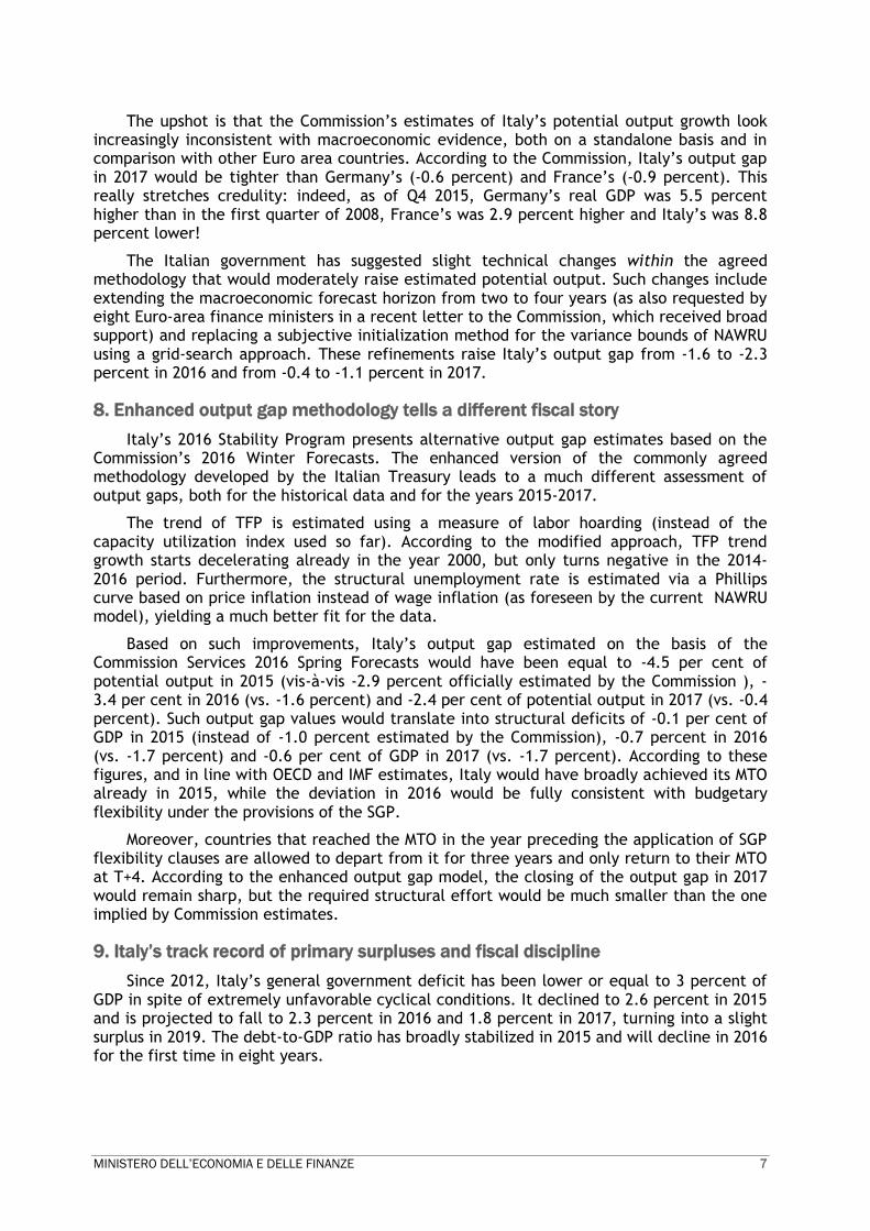
The upshot is that the Commission’s estimates of Italy’s potential output growth look increasingly inconsistent with macroeconomic evidence, both on a standalone basis and in comparison with other Euro area countries. According to the Commission, Italy’s output gap in 2017 would be tighter than Germany’s (-0.6 percent) and France’s (-0.9 percent). This really stretches credulity: indeed, as of Q4 2015, Germany’s real GDP was 5.5 percent higher than in the first quarter of 2008, France’s was 2.9 percent higher and Italy’s was 8.8 percent lower!
The Italian government has suggested slight technical changes within the agreed methodology that would moderately raise estimated potential output. Such changes include extending the macroeconomic forecast horizon from two to four years (as also requested by eight Euro-area finance ministers in a recent letter to the Commission, which received broad support) and replacing a subjective initialization method for the variance bounds of NAWRU using a grid-search approach. These refinements raise Italy’s output gap from -1.6 to -2.3 percent in 2016 and from -0.4 to -1.1 percent in 2017.
8. Enhanced output gap methodology tells a different fiscal story
Italy’s 2016 Stability Program presents alternative output gap estimates based on the Commission’s 2016 Winter Forecasts. The enhanced version of the commonly agreed methodology developed by the Italian Treasury leads to a much different assessment of output gaps, both for the historical data and for the years 2015-2017.
The trend of TFP is estimated using a measure of labor hoarding (instead of the capacity utilization index used so far). According to the modified approach, TFP trend growth starts decelerating already in the year 2000, but only turns negative in the 2014-2016 period. Furthermore, the structural unemployment rate is estimated via a Phillips curve based on price inflation instead of wage inflation (as foreseen by the current NAWRU model), yielding a much better fit for the data.
Based on such improvements, Italy’s output gap estimated on the basis of the Commission Services 2016 Spring Forecasts would have been equal to -4.5 per cent of potential output in 2015 (vis-à-vis -2.9 percent officially estimated by the Commission ), -3.4 per cent in 2016 (vs. -1.6 percent) and -2.4 per cent of potential output in 2017 (vs. -0.4 percent). Such output gap values would translate into structural deficits of -0.1 per cent of GDP in 2015 (instead of -1.0 percent estimated by the Commission), -0.7 percent in 2016 (vs. -1.7 percent) and -0.6 per cent of GDP in 2017 (vs. -1.7 percent). According to these figures, and in line with OECD and IMF estimates, Italy would have broadly achieved its MTO already in 2015, while the deviation in 2016 would be fully consistent with budgetary flexibility under the provisions of the SGP.
Moreover, countries that reached the MTO in the year preceding the application of SGP flexibility clauses are allowed to depart from it for three years and only return to their MTO at T+4. According to the enhanced output gap model, the closing of the output gap in 2017 would remain sharp, but the required structural effort would be much smaller than the one implied by Commission estimates.
9. Italy’s track record of primary surpluses and fiscal discipline
Since 2012, Italy’s general government deficit has been lower or equal to 3 percent of GDP in spite of extremely unfavorable cyclical conditions. It declined to 2.6 percent in 2015 and is projected to fall to 2.3 percent in 2016 and 1.8 percent in 2017, turning into a slight surplus in 2019. The debt-to-GDP ratio has broadly stabilized in 2015 and will decline in 2016 for the first time in eight years.

8 MINISTERO DELL’ECONOMIA E DELLE FINANZE
This result was accomplished through primary surpluses that on average have been the largest in the EU during the 2009-2015 period. The Italian government has followed a growth-friendly approach to fiscal consolidation, combining a remarkable structural reform effort with a significant reduction of the tax wedge on labor and a durable improvement in the efficiency and quality of public expenditure at all levels of government. Growth-enhancing expenditure on R&D, innovation, education and essential infrastructure projects has been increased.
This is consistent with the provisions of Regulation 1467/97, which considers “the record of adjustment towards the medium-term budgetary objective, the level of the primary balance and developments in primary expenditure, both current and capital, the implementation of policies in the context of the prevention and correction of excessive macroeconomic imbalances, the implementation of policies in the context of the common growth strategy of the Union and the overall quality of public finances, in particular the effectiveness of national budgetary frameworks” as relevant factors in assessing the medium term budgetary position.
Compliance with the preventive arm was considered in the 2015 Opinion by the Commission, and subsequently by the EFC, as one of the relevant factors in assessing the overall budgetary position. The 2016 Stability Program ensures compliance with the preventive arm of the SGP in 2016. Compliance with the preventive arm in 2017 would also be assured if calculations were based on more realistic estimates of Italy’s potential output.
10. Long-term debt sustainability
According to calculations by the Commission, thanks to the reforms already enacted in age-related expenditure, Italy has the highest long-term sustainability indicator (S2) among EU countries. Moreover, in the simulations presented in the Fiscal Sustainability Report, the probability that Italy’s debt in 2020 will be higher than in 2015 level is one of the lowest, second only to Germany.
Italy can also boast one of the most favorable debt-maturity structures among EU countries. Considering overall private and public debt, as well as contingent liabilities, the position of Italy is in line with major EU countries.
11. Costs of immigration and refugee crisis
In recent years Italy incurred extraordinary costs equivalent to 0.2 percent of GDP on an annual basis as it dealt with a large wave of immigrants and asylum seekers. This effort should be taken into account when assessing deficit and debt developments, as the government argued in the 2016 Draft Budgetary Plan.
In conclusion
In a spirit of compliance with the EU fiscal rules, we urge the Commission to consider the factors summarized in this note in order to appropriately assess Italy’s fiscal stance and prospects for public debt reduction in the coming years.

MINISTERO DELL’ECONOMIA E DELLE FINANZE 9
I. CYCLICAL CONDITIONS
I.1 THE ITALIAN ECONOMY AND THE INTERNATIONAL ENVIRONMENT
In 2015, real GDP growth returned into positive territory after three consecutive years
of contraction. The fall of GDP with respect to the Q1 2008 peak is still close to 9 percent.
Contrary to the consensus view dominating until last spring, Italy’s economic recovery
has been driven by domestic demand. Having already risen in 2014, private consumption
accelerated further, thanks to improved labour market conditions, a recovery in real
disposable income, and improvements in financing conditions. On the other hand, the
policies for holding down the general government expenditure on employee compensation
and intermediate consumption were successful in reducing real public consumption, the
trend of which has been negative, without interruption, since 2011. Fixed Investment posted
uneven gains: purchase of transport vehicles took the lead, but investment on plant and
equipment remained sluggish; the construction sector appears on the verge of recovery
after a prolonged and deep contraction.
The Italian recovery was overall resilient to the gradually deteriorating international
environment, as external stimulus gradually receded. The depreciation of the euro,
especially in nominal effective terms, was less intense than expected, international trade
plummeted in the second half of 2015 and it is only very slowly recovering and financial
markets, very positive until the first half of 2015, are currently subject to volatility. The
drop in oil prices, though supportive for households’ disposable income, led to unwanted
side effects, further depressing demand from emerging economies. Excess productive
capacity, a large fraction of with is located in China, and the slump in commodity prices
added to deflationary pressures by driving down the price of manufactured goods.
In this economic environment, an excessively restrictive fiscal policy stance may
aggravate deflation pressures. The Commission has commendably focused the European
Semester on the achievement of a fiscal stance that is appropriate for the Euro area as a
whole. However, the budget and debt rules that were put in place to strengthen the
framework of economic governance in the aftermath of the economic and financial crisis
force deficit countries to follow tight fiscal policies, while countries that enjoy ‘fiscal space’
are not making significant use of it. The aggregate outcome in terms of fiscal policy is not
too far from what the Commission deems appropriate for the Euro area as a whole only
because some countries are deviating from their respective Council recommendations.
Moreover, cutting budget deficits in the presence of rigidities in current expenditure
has led member states to curtail public investment. This is one of the key reasons why
overall investment is falling short of what would be needed to achieve a sustained economic
recovery.
Overall, expansionary monetary policies were less effective than expected in sustaining
the recovery of investment; recent intervention however was able to stabilize financial
markets and, thanks to specific measures, should provide more stimulus to investment.
Against this background, the Italian government took stock of the less dynamic
exogenous environment and prudently revised its projections reducing GDP growth forecast

10 MINISTERO DELL’ECONOMIA E DELLE FINANZE
for both 2016 and 2017. Under the new policy macroeconomic scenario growth relies even
more on domestic demand; in order to consolidate the recovery and to make it resilient it is
therefore essential to preserve this source of growth. The policy scenario rests also on a
fiscal policy that is still rigorous, but more focused on promoting economic activity and
employment.
The new budgetary path adds a few decimal points to growth and, more important, it
provides a buffer against the possibility that headwinds coming from a further deterioration
of the exogenous environment brings back the Italian economy to the brink of deflation.
The Italian government is confident that its growth and public finance targets are
realistic. However, risks to the outlook are still tilted to the downside. The degree of
tightening in fiscal policy must be commensurate to these risks so that the recovery gains
momentum.
I.2 SENSITIVITY ANALYSIS: WORSENING GLOBAL CONDITIONS AND FISCAL TIGHTENING
This section shows the results of simulations carried out with the Italian Treasury
econometric model ITEM in order to analyse risks to the ongoing recovery and the
appropriate fiscal policy stance to be followed under these circumastances. The baseline
2016 simulation is consistent with the official growth and public finance scenario published
in the Stability Program. In the baseline scenario the public debt to GDP ratio matches
exactly the path of the official forecast, exhibiting an accelerating decline.
The first alternative scenario (yellow line) entails a more protracted stagnation of
world trade and a subdued behavior of international prices. The growth rates in the demand
for Italian goods and in producer prices (both weighted for the share of each country in
Italian exports) are reduced by 1 percent and 1.5 percent respectively for two years. Beyond
that, their growth rates match that of the baseline simulation. No additional shock is
implemented, although a more complex scenario (such as one incorporating financial
stresses) could be also simulated. At the same time, monetary policy is left unchanged with
respect to baseline, as there is arguably limited room for further accommodation.
The second alternative scenario (A2, light green line) builds on the weaker international
setting incorporated in the first one and adds to it a permanent fiscal adjustment of 0.5
percentage points of GDP taking place in the year 2017. The fiscal contraction equals the
amount needed to reach full formal compliance with the preventive arm of the growth and
stability pact.
The fiscal adjustment takes place on the expenditure side of the public sector budget
and it is achieved mostly by cutting purchases of intermediate goods, investment in volume
terms and – to a lesser extent – employment. There are well grounded reasons to assume
such a composition. The repeal of safeguard clauses, will be partially compensated by
expenditure cuts and to some extent by a possible revision of tax expenditures. Both
categories entail reductions either in prices (induced for instance by the foreseen
improvement of the public procurement system) or in transfers to the private sector of the
economy. Additional cuts of the same kind would be unfeasible within a short timeframe,
therefore the required savings would have to be achieved via more aggressive and
potentially recessionary measures.

MINISTERO DELL’ECONOMIA E DELLE FINANZE 11
The results of the simulation suggest the following. First, protracted weakness of global
economic conditions would further delay the foreseen reduction of the debt to GDP ratio
but Italy’s public debt would remain fully sustainable. By the year 2018, debt reduction
would resume at full speed. Second, additional fiscal adjustment does not lead to a faster
reduction of the ratio; on the contrary, in the short term it delays it. These results should
be further qualified. It should be noted that they originate from the econometric model and
there is a wide strand of the economic literature showing that during “bad times” fiscal
multipliers are higher than those generated by traditional models1. The self-defeating
outcome just laid out, therefore, could be significantly larger than suggested by this
simulation.
A third scenario is, indeed built assuming a fiscal multiplier 50 percent higher than that
generated by the econometric model and equal approximately to 1.2. The third (orange)
line shows that in this case the public debt to GDP ratio would stay above the no
intervention scenario for the whole simulation period.
FIGURE 1.1 – DEBT- TO-GDP RATIO
Source: MEF simulations with ITEM
I.3 DEFLATIONARY PRESSURES AND MONETARY ACCOMMODATION
Global deflationary pressures have intensified over the past two years, owing in
particular to increased geopolitical tensions, the drop in energy and commodity prices and a
marked slowdown in oil-producing countries and in large emerging economies such as China,
Russia and Brazil. These developments have severely complicated the task of reducing debt-
to-GDP ratios for countries like Italy that were just beginning to recover from a recession of
unprecedented proportions.
1 For a review see the Update of the Economic and Financial Document 2015,pages 25 to 27.
http://www.dt.tesoro.it/modules/documenti_it/analisi_progammazione/documenti_programmatici/Update_of_the_2015_EFD_.pdf
122
124
126
128
130
132
134
2015 2016 2017 2018 2019
Baseline
Low growth international scenario
Low growth international scenario + fiscal consolidation
Low growth international scenario + fiscal consolidation (mult. 1.2)

12 MINISTERO DELL’ECONOMIA E DELLE FINANZE
The ECB has responded to intensifying deflation risks by escalating monetary policy
accommodation. Still, the ECB’s policy response has not totally offset the adverse impact of
changing economic circumstances on Italy’s debt-to-GDP ratio.
This contention is supported by running the following simulation on the ITEM model. We
rewind to early 2014, when oil prices were still above 100 dollars per barrel and
expectations concerning growth in world trade were moderately optimistic (and European
exports to Russia were still at a high though declining level). We project the course of the
Italian economy in 2014-2018 based on the exogenous variables and interest rate
expectations that were employed in Italy’s 2014 Stability Program. At the time (late March
2014), these values were close to the consensus forecast and to the projections of the main
international organizations. Interest rates, exchange rates and commodity and energy prices
were based on market levels and forward rates.
TABLE 1.1 – EXOGENOUS ECONOMIC VARIABLES AND MONETARY CONDITIONS IN DEF 2014 AND DEF 2016.
Exogenous economic variables
2014 2015 2016 2017 2018 2019
Trade weighted world demand (% change) DEF 2016 3.66 2.94 2.93 4.46 4.49 4.24
DEF 2014 4.27 4.55 4.75 5.00 5.03 4.99
Oil (level) DEF 2016 96.5 50.9 39.4 45.7 48.1 49.8
DEF 2014 100.7 99.6 99.6 99.6 99.6 99.6
Trade weighted external price (% change) DEF 2016 -0.31 -2.19 0.65 1.85 2.02 2.04
DEF 2014 1.19 2.17 2.21 2.04 1.82 1.79
Raw materials price (% change) DEF 2016 17.0 -19.6 -8.8 3.9 4.0 3.6
DEF 2014 2.25 0.27 2.41 2.51 2.22 2.19
Monetary Conditions
2014 2015 2016 2017 2018 2019
Exchange rate ($/€) (level) DEF 2016 1.33 1.11 1.1 1.11 1.11 1.11
DEF 2014 1.36 1.36 1.36 1.36 1.36 1.36
Nominal effective exchange rate (% change) DEF 2016 0.98 -3.78 1.85 -0.03 0.00 0.00
DEF 2014 1.62 -0.07 0.00 0.00 0.00 0.00
Euribor 3m (level) DEF 2016 0.21 -0.02 -0.16 -0.16 0.14 0.54
DEF 2014 0.30 0.29 0.28 0.46 1.4 2.07
BTP 10 years (level) DEF 2016 2.89 1.76 1.74 1.92 2.22 2.51
DEF 2014 3.62 3.64 3.33 3.19 3.26 3.22
Spread Btp-Bund (Level) DEF 2016 1.73 1.21 1.46 1.70 1.85 1.98
DEF 2014 1.95 1.49 1.22 1.03 1.00 1.00
Source: MEF.
We then ran a second simulation using the actual path of the exogenous variables up to
early 2016 and then extending such path with the projections employed in this year’s
Stability Program through to end-2018. This alternative scenario incorporates the effects of
quantitative easing (QE) and policy rate cuts implemented by the ECB in mid-2014 to early
2016, which were not anticipated by the markets at the beginning of 2014.
Comparing the two simulations obtained with ITEM, it is thus possible to assess the net
impact of the change in global economic conditions on nominal GDP growth and on the debt-
to-GDP ratio including the beneficial impact of ultra-accommodative monetary policy and

MINISTERO DELL’ECONOMIA E DELLE FINANZE 13
other factors that contributed to easing monetary conditions (e.g. US Federal Reserve rate
hikes and expectations thereof).
In presenting the simulation results, we isolate the effects of the worsening of global
economic conditions (world trade growth and commodity prices) from those of easier
monetary conditions (including the depreciation of the euro exchange rate).
TABLE 1.2 – SIMULATION RESULTS FOR GDP AND DEBT TO GDP RATIO
Nominal GDP
% deviations from baseline scenario
2014 2015 2016 2017 2018
Exogenous economic variables -0.27 -0.77 -1.53 -2.38 -2.81
Monetary Conditions 0.06 0.65 0.88 0.77 0.49
Total -0.21 -0.12 -0.64 -1.61 -2.32
Debt/GDP
Differences from baseline scenario
2014 2015 2016 2017 2018
Exogenous economic variables 0.40 1.32 3.00 5.08 6.74
Monetary Conditions -0.13 -1.29 -2.31 -3.02 -3.55
Total 0.27 0.03 0.68 2.06 3.19
Source: MEF simulations with ITEM
The simulation suggests that easier monetary conditions boost nominal GDP by 0.65
percentage points in 2015 and 0.88 points in 2016. The impact then declines gradually to
0.49 points in 2018, the last year of the simulation, compared to the ‘early 2014’ scenario.
In terms of the impact on the public finances, simulation results point to an improvement in
the debt-to GDP ratio stemming directly from a reduction of interest rates paid by the
government and indirectly from the expansionary impulse. The debt-to-GDP reduction with
respect to the baseline scenario amounts to -1.29 percentage point in 2015, -2.31 points in
2016 and -3.55 points in 2018.
FIGURE 1.2 – NOMINAL GDP - % DEVIATIONS FROM BASELINE SCENARIO
Source: MEF simulations with ITEM
-6.0
-5.0
-4.0
-3.0
-2.0
-1.0
0.0
1.0
2.0
2013 2014 2015 2016 2017 2018
Exogenous economic variables
Exogenous economic
variables_anemic growth
Monetary Conditions

14 MINISTERO DELL’ECONOMIA E DELLE FINANZE
FIGURE 1.3 – DEBT/GDP - DIFFERENCES FROM BASELINE SCENARIO
Source: MEF simulations with ITEM
By contrast, the overall effect of changes in the pattern of the world demand,
international manufacturing prices and oil prices (whose drop represents a stimulus to
economic activity) with respect to the ‘early 2014’ scenario is a reduction of nominal GDP
with respect of the baseline scenario. The latter is equal to -0.27 percentage points in 2014,
-0.77 points in 2015 and -1.53 points in 2016. These contractionary effects impact the debt-
to-GDP ratio, which increases by 0.40 percentage points in 2014, 1.32 points in 2015 and 3.0
points in 2016.
Thus, our findings suggest that although the easing of monetary conditions has had a
significant positive impact on the Italian economy and public finances, it only partially
offset the negative effects on the economy and debt-to-GDP ratio of the deterioration in the
international economic environment. We also observe that savings on interest payments
increase over time, but only gradually.
If we extend the ‘lowflation’ scenario to 2017-2018, i.e. we assume that, unlike in the
2016 Stability Program scenario, world manufacturing and oil prices and the growth in
international trade do not increase materially compared to the recent trend, the simulation
yields an even larger adverse impact on Italy’s debt-to-GDP ratio. Namely, if the growth
rate of demand for Italian exports remains at 3 per cent for the whole simulation period,
the price of manufactured products grows 1.5 percentage points below the expected path
and the oil price remains at current level (anemic growth), the debt-to-GDP ratio reaches a
level 6.7 percentage points higher than in the ‘early 2014’ scenario.
I.4 ESTIMATION OF OUTPUT GAP AND POTENTIAL GROWTH
Since 2012, after the end of the Excessive Deficit Procedure (EDP) and the start of the
subsequent three year period of transition regime for the Debt Rule, the Italian economy has
been going through one of the most severe and lengthy recessions in its history. Real GDP
-6
-4
-2
0
2
4
6
8
10
12
2013 2014 2015 2016 2017 2018
Exogenous economic variables
Exogenous economic variables_anemic
growth
Monetary Conditions

MINISTERO DELL’ECONOMIA E DELLE FINANZE 15
fell by 2.8 per cent in 2012, 1.7 in 2013, and 0.3 per cent in 2014. Real growth only returned
into positive territory in 2015, attaining a rate of 0.8 per cent.
According to the 2016 Commission services Spring forecasts, Italy’s real GDP should
grow by 1.1 per cent (vis-à-vis 1.2 per cent forecast by the Italian Government) and 1.3 per
cent in 2017 (vis-à-vis 1.4 per cent projected by the Italian Government).
Estimated potential growth has remained in negative territory both as a result of the
crisis and as a consequence of the pro-cyclicality embedded in the commonly agreed
methodology. On the basis of the 2016 Commission services Spring Forecasts, potential
growth is estimated to have recorded negative rates of -1.1 per cent in 2012, -0.8 per cent
in 2013, -0.7 per cent in 2014 and -0.3 per cent in 2015, end of the debt rule transitional
period. Over the forecast horizon, potential growth will keep being negative and equal to -
0,2 per cent in 2016 and slightly positive, 0.1 per cent, in 2017. Potential growth estimated
by the Italian Government on the basis of the same agreed methodology but over a longer
forecast horizon, presents similar pattern up till 2017. In the following two years, potential
growth is expected to accelerate reaching 0.5 per cent in 2019.
The analysis of the underlying factors shaping potential growth shows that the
contribution coming from labour, after the large and negative record of 2012 (equal to -0.9
per cent), is expected to resume fast. However, its contribution will be almost nil both in
2015 and 2016 and slightly positive (0.2 per cent) only in 2017. Quite controversially, Total
Factor Productivity (TFP), has been delivering persistently negative support to potential
growth for more than a decade (from 2002 to 2015) and over the two years forecast horizon
(2016 and 2017).
In spite of the negative potential growth rate, output gaps posted historical high levels,
equaling -4.3 per cent of potential GDP in 2013 and -3.9 per cent of potential output in
2014. As of 2015, in spite of the deflationary trends that are still affecting the country, the
output gap is estimated to close very fast, attaining -2.9 per cent last year, almost halving
in 2016 (-1.6 per cent of potential output) and reaching -0.4 per cent in 2017. According to
the Commission services matrix specifying the annual fiscal adjustment towards the MTO,
such cyclical conditions should be defined as bad times in 2016 and normal times in 2017
corresponding to a required annual fiscal adjustment, respectively, of 0.5 percentage points
in 2016 and above 0.5 percentage points of GDP in 20172.
The Italian Government is of the opinion that the severe cyclical conditions recorded
over the period 2012-2014 have not been properly internalized in the commonly agreed
production function methodology, resulting in a protracted fall in potential output which
contributes to the quick closure of the output gap over the period 2016-2017, in spite of the
still large existing capacity utilization. As the output gap closes quickly also the required
fiscal adjustment according to the so-called matrix is fast increasing to take into account of
the supposedly improvements in cyclical conditions.
According to the Government, the assessment of the cyclical conditions carried out
through the output gaps stemming from the commonly agreed methodology is, to some
extent, pro-cyclical and not line with macroeconomic intuition. Moreover, the estimation
may be flawed with different statistical shortcomings which may render the methodology
2 These benchmark does not include all the flexibility exceptions allowed by the Stability and Growth Pact. For details,
see: European Commission, Communication from the Commission- Making the best use of the flexibility within the existing rules of the SGP, January 13th, 2015

16 MINISTERO DELL’ECONOMIA E DELLE FINANZE
basically not suited for providing an unbiased assessment of past and future potential
growth dynamics.
As already pointed out in the 2016 Stability Programme, when applied to Italian data,
the commonly agreed production function performs poorly with respect to the estimation of
the Non-Accelerating Rate of Wage Unemployment (NAWRU) and in the extrapolation of the
trend and cyclical components of Total Factor Productivity (TFP). To address both issues,
the Italian Treasury proposed an enhanced production function model which only slightly
departs from the commonly agreed one. The details and the results of such model are based
on 2016 Commission Services Spring Forecasts and are reported in the Focus below.
As far as NAWRU is concerned, the main shortcomings are related to: 1) the intrinsic
pro-cyclicality of the estimates deriving from the judgmental selection of the initialisation
bounds; 2) the very low statistical significance of the Phillips curve which presents a R-
square statistic close to zero.
Regarding to the latter point, it is possible to refer to the alternative model proposed in
the Focus. By contrast, as far as the pro-cyclicality of the NAWRU is concerned, the
following argument may propose one, among many, explanations.
It is important to recall that in order to carry out the NAWRU estimations through the
bivariate Kalman filter model, the ex-ante identification of the initialization parameters for
the latent factors and, in particular, the variances of the shocks to the trend and cyclical
components and of the stochastic process that drives the Phillips curve, is required.
Although the estimation method is rather sophisticated, the selection of the upper and
lower limits (bounds) of the four variances of the shocks to the trend, the slope, the cycle
and the Phillips curve is crucial for the determination of the level and the trend of the
NAWRU as, in the case of Italy, the model mostly set the estimated variances exactly at the
upper or lower values of such bounds. Such values are chosen on a judgmental basis,
producing somehow a sort of induced pro-cyclicality.
To minimize the “cost of judgement” and the “bias” in the selection of the NAWRU
variance bounds, the Italian Treasury conceived an empirical method, based on a an
iterative grid search procedure3, which allows to choose the initialisation bounds in an
optimal manner (from a statistical point of view)4.
Moreover, on the basis of the Treasury Department grid search procedure, based on 800
iterations, it is possible to derive, for each point in time over the whole estimation horizon
(1967-2017), a frequency distribution of each NAWRU estimate. According to our
calculations based on the 2016 Spring Forecasts, the NAWRU obtained with the selected
optimal bounds deviates from the median of each frequency distribution less than the
NAWRU estimated by the European Commission whose bounds are based on a judgmental
selection (Figure I.4). The deviation from the median is higher in the case of Commission
estimates especially in correspondence to the unemployment rates turning points (for
instance, in 1996 which represents a peak, in 2006 which is a minimum and in 2014-2015
which is the following cyclical peak).
3 See the 2015Italy’s Stability Programme, available on:
http://www.dt.tesoro.it/modules/documenti_en/analisi_progammazione/documenti_programmatici/PdS_2015_xENx.pdf
4 In details, the optimal bounds underlying the 2016 Spring Forecasts, are: 0 (LB trend); 0.025 (LB slope); 0 (LB cycle);
0.1 (UB trend); 0.03 (UB slope); 0.15 (UB cyle)

MINISTERO DELL’ECONOMIA E DELLE FINANZE 17
FIGURE I.4: DISTANCE TO THE MEDIAN OF THE NAWRU ESTIMATES DISTRIBUTION
.00
.04
.08
.12
.16
.20
90 92 94 96 98 00 02 04 06 08 10 12 14 16
Best NAWRU (selected with Grid search)
NAWRU Spring Forecast 2016
Source: European Commission 2016 Spring Forecasts and own elaborations.
Note: The Italian Treasury has carried out an analysis of the NAWRU starting with the values of the bounds used by the European Commission in the 2016 Spring Forecast. A number of alternative combinations of lower and upper bounds for the variances of latent factors (about 800) has been constructed around such values through the grid search iterative procedure. Then, on the basis of a model selection criteria an optimal combination of the initial variances of the latent factors have been selected, which provides a less pro-cyclical results and a general improvement of the statistics for the NAWRU estimates.
In conclusion, the optimal NAWRU obtained through the grid search procedure is very
close to the center of the yearly estimates distribution, whereas the NAWRU of the
Commission lies more on the tails of the distributions. As a consequence, the judgmental
selection of the NAWRU bounds by the Commission services determines an intrinsic pro-
cyclicality of their estimates especially around unemployment rates turning points.
Accordingly, the policy of minimizing historical revisions among Commission services
forecast vintages by opportunely selecting the variance bounds contributes to perpetuate
such pro-cyclicality over time at the expenses of the ability to provide more plausible
results from the macroeconomic point of view.
As far as TFP is concerned, its measurement for Italy is subject to some relevant
drawbacks related to: 1) the current estimates of the growth rate of the TFP trend which,
quite counterintuitively, are negative as of 2002, thus contributing to the reduction of both
the levels and the growth rates of potential output; 2) the statistical properties of the
capacity utilization indicator (the so-called CUBS) and its relevance for the determination of
output gaps revisions.
Both issues are extensively dealt with in the Focus where the enhanced potential output
estimates of the Italian treasury are presented. However, with reference to the relation
between the CUBS indicator and output gap revisions it is worth pointing out how output
gaps in Commission forecasts have been significantly changing as a result of a minimal
update of the CUBS index. For instance, the introduction of the “anomalous” observation of
the CUBS indicator for 2015 carried out last September, pointing to a sudden increase in
sentiment indicators not matched by actual production values, determined a statistical
revision of the output gaps in the Commission forecasts which cannot be explained on the
basis of macroeconomic intuition.
18 MINISTERO DELL’ECONOMIA E DELLE FINANZE
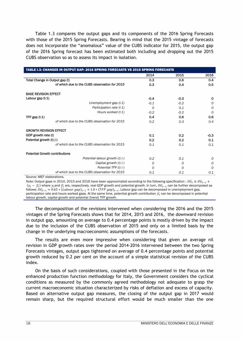
Table 1.3 compares the output gaps and its components of the 2016 Spring Forecasts
with those of the 2015 Spring Forecasts. Bearing in mind that the 2015 vintage of forecasts
does not incorporate the “anomalous” value of the CUBS indicator for 2015, the output gap
of the 2016 Spring forecast has been estimated both including and dropping out the 2015
CUBS observation so as to assess its impact in isolation.
TABLE I.3: CHANGES IN OUTPUT GAP: 2016 SPRING FORECASTS VS 2015 SPRING FORECASTS
2014 2015 2016
Total Change in Output gap (t) 0.3 0.6 0.4
of which due to the CUBS observation for 2015 0.3 0.4 0.5
BASE REVISION EFFECT
Labour gap (t-1) -0.4 -0.3 0
Unemployment gap (t-1) -0.1 -0.2 0
Participation rate (t-1) 0 0.1 0
Hours worked (t-1) -0.2 -0.2 0
TFP gap (t-1) 0.4 0.6 0.6
of which due to the CUBS observation for 2015 0.2 0.3 0.4
GROWTH REVISION EFFECT
GDP growth rate (t) 0.1 0.2 -0.3
Potential growth (t) (-) 0.2 0.2 0.1
of which due to the CUBS observation for 2015 0.1 0.1 0.1
Potential Growth contributions
Potential labour growth (t) (-) 0.2 0.1 0
Capital growth (t) (-) 0 0 0
Potential TFP (t) (-) 0 0 0
of which due to the CUBS observation for 2015 0.1 0.1 0.1
Source: MEF elaborations.
Note: Output gaps in 2014, 2015 and 2016 have been approximated according to the following specification : 𝑂𝐺𝑡 ≅ 𝑂𝐺𝑡−1 + (𝑦𝑡 − 𝑦�̅�) where 𝑦𝑡and 𝑦�̅� are, respectively, real GDP growth and potential growth. In turn, 𝑂𝐺𝑡−1 can be further decomposed as
follows: 𝑂𝐺𝑡−1 = 0.65 ∗ (𝐿𝑎𝑏𝑜𝑢𝑟 𝑔𝑎𝑝)𝑡−1 + 1.0 ∗ (𝑇𝐹𝑃 𝑔𝑎𝑝)𝑡−1. Labour gap can be decomposed in unemployment gap,
participation rate and hours worked gaps. At the same time, potential growth contribution 𝑦�̅� can be decomposed in potential
labour growth, capital growth and potential (trend) TFP growth.
The decomposition of the revisions intervened when considering the 2016 and the 2015
vintages of the Spring Forecasts shows that for 2014, 2015 and 2016, the downward revision
in output gap, amounting on average to 0.4 percentage points is mostly driven by the impact
due to the inclusion of the CUBS observation of 2015 and only on a limited basis by the
change in the underlying macroeconomic assumptions of the forecasts.
The results are even more impressive when considering that given an average nil
revision in GDP growth rates over the period 2014-2016 intervened between the two Spring
Forecasts vintages, output gaps tightened on average of 0.4 percentage points and potential
growth reduced by 0.2 per cent on the account of a simple statistical revision of the CUBS
index.
On the basis of such considerations, coupled with those presented in the Focus on the
enhanced production function methodology for Italy, the Government considers the cyclical
conditions as measured by the commonly agreed methodology not adequate to grasp the
current macroeconomic situation characterized by risks of deflation and excess of capacity.
Based on alternative output gap measures, the closing of the output gap in 2017 would
remain sharp, but the required structural effort would be much smaller than the one
MINISTERO DELL’ECONOMIA E DELLE FINANZE 19
implied by the current Commission estimates. On the basis of the enhanced methodology,
Italian economy would indeed experience exceptional bad times in 2014 and 2015, very bad
times in 2016 and bad times in 2017.
The estimation of potential output: an enhanced methodology for Italy.
Given its relevance in determining structural budget balances both under the framework of the Stability
and Growth Pact and under the national legislation (Law n. 243/2012), the agreed production function
methodology shared at the EU level to gauge potential output and output gaps has come increasingly
under scrutiny in recent years. Both the European Commission and the Output Gap Working Group
(OGWG), in charge of monitoring the agreed methodology, have recognised the existence of theoretical
and econometrical drawbacks and have largely discussed possible adjustments to the model. However,
in some cases, like the Italian one, problems still remain.
According to the mandate of the Output Gap Working Group (OGWG), the commonly agreed
methodology should respect the following principles: a) It has to be relatively simple, fully transparent
and stable. The trend extraction methods should be based on economic as well as statistical principles
with the key inputs and outputs clearly defined; b) It should strive for equal treatment for all EU Member
States, whilst in exceptional circumstances recognising country-specific characteristics; c) It should
provide an unbiased assessment of the past and future potential growth in the EU Member States,
while aiming to include the effects of all adopted structural reforms; d) It should aim at limiting the pro-
cyclicality of potential growth estimates.
As far as Italy is concerned, the Government is of the opinion that the current agreed methodology is
not suited for providing an unbiased assessment of past and future potential growth. Results are pro-
cyclical and not in line with macroeconomic intuition. More in details, when applied to Italian data, the
commonly agreed production function performs poorly with respect to the estimation of the Non-
Accelerating Rate of Wage Unemployment (NAWRU) and in the extrapolation of the trend and cyclical
components of Total Factor Productivity. On both items, this note puts forward some enhanced
solutions based on a slight modification of the commonly agreed methodology. The large volatility in the
results vis-à-vis those produced by the Commission proves that the model is not stable neither over the
historical period nor over the forecast horizon.
A new Phillips curve for the estimation of Italian potential GDP
The Non-Accelerating Wage Rate of Unemployment (NAWRU) is a latent variable representing the
unemployment rate consistent with no change in wage inflation. Given this definition, the NAWRU for
Italy is estimated in the commonly agreed methodology through a very stylized model. A Kalman filter is
applied to the series of the unemployment rate and to the so-called Phillips curve, i.e. the equation that
expresses the inverse relationship between wage inflation and a concurrent and two-period lags
measure of cyclical unemployment5.
Recent empirical analyses have shown that the wage/unemployment relationship featured by the
Phillips curve may have weaken over past decades and, in particular, during the recent financial crisis6.
5 For the complete specification of the commonly agreed methodology used for the NWRU estimation see Section III.1 of
the Methodological Note attached to the EFD 2016.
6 Considering the current level of interest rates and low inflation, the relationship between the unemployment rate and labour cost seems to have lost significance. Indeed, despite the sizeable increase in unemployment during the most recent recession, the effects on wage inflation have been modest. Some empirical studies estimate a gradual levelling of the curve due to the fact that price expectations have been anchored to the inflation targets declared and pursued by the respective central banks. Other researches have shown how the traditional Phillips curve tends to indicate a weakening of the relationship between unemployment and wages (or price inflation) because the traditional curve overlooks the broader weight assumed by long-term unemployment, which, since it cannot be reabsorbed quickly, contributes to creating additional hysteresis. With reference to the first effect, see: Ball L. Mazumder S., (2015) A Phillips Curve with Anchored Expectations and Short-Term
Unemployment, IMF Working Paper, WP/15/39, available at:
http://www.imf.org/external/pubs/ft/wp/2015/wp1539.pdf. See also: Rusticelli E., Turner D. Cavalleri M.C. (2015) Incorporating Anchored Inflation expectations in the Phillips Curve and in the derivation of OECD measures of the unemployment gap, OECD Working papers. With reference to the effect of long-term inflation, see: Elena Rusticelli, (2014),
FO
CU
S

20 MINISTERO DELL’ECONOMIA E DELLE FINANZE
In recent years, considerable increases in the unemployment rate experienced in some countries,
including Italy, have not been matched by correspondent reduction in wage inflation in line with what
would have been foreseen on the basis of the mechanisms underlying the Phillips curve.
In addition, in Italy's case, the Phillips curve model used for the estimation of the NAWRU as part of the
methodology agreed at the European level for computing the output gaps and structural balances7 has,
in most cases, produced estimates that are not robust from a statistical point of view and not entirely
in line with macroeconomic intuition.
For instance, according to the 2016 Spring Forecasts, the NAWRU for Italy is expected to increase by
0.5 percentage points from 10.4 per cent of 2015 to 10.9 per cent of 2017 in spite of the fact that: 1)
over the same time horizon, the unemployment rate is projected to fall of 0.7 percentage points; 2)
wage inflation is expected to be almost nil; 3) the tax wedge has fallen from 44.7 per cent in 2013 to
42.4 per cent in 2014 as a result of the implementation of structural reforms.
Furthermore, in the Spring Forecast 2016, even though the related coefficients that link wage inflation
to the unemployment gap are highly significant, the entire Phillips curve model is marked by a very low
coefficient of correlation R2 whose value is just above zero.
In an attempt to improve the fit of the model, it is possible to use an alternative specification of the
Phillips curve, in which, in line with the approach previously adopted by other international
organisations (such as the OECD and IMF), the endogenous variable currently represented by the series
that measures the acceleration of wage inflation is to be substituted with the series that measures
price inflation.
More specifically, the model has been re-estimated, by substituting the equation currently used by the
European Commission for the estimation of the Phillips curve (see formula (8) of the Methodological
Note in Section III.1 of this document) with the following formula:
Pt = + 1Gt + 2Gt-1 + 3Gt-2 + MGSt + 4t 4t ~ N(0, var4))
where P= the inflation rate calculated on the consumption deflator, Gt= unemployment gap and MGS=
weight of imported inflation on the quota of domestic demand. The introduction of an exogenous
variable capable of capturing the effects of import prices is in line with the OECD model and with the
theoretical formula adopted by the European Commission8.
When using such specification for the Phillips curve, the model moves from the estimation of the Non-
Accelerating Wage Rate of Unemployment (NAWRU) to the estimation of the Non-Accelerating Inflation
Rate of Unemployment (NAIRU) although remaining within the framework used by the European
Commission.
The results reported in the table and figures below show a general improvement in the estimates of
structural unemployment when compared with the results obtained by the European Commission for
the Spring Forecast 2016 (see log likelihood figure), as well as a considerable increase in the goodness
of fit of the Phillips curve witnessed by the huge increase in the R2 statistic (equal to approximately 47
per cent under the new specification).
Rescuing the Phillips curve: Making use of long-term unemployment in the measurement of the NAIRU, OECD Journal: Economic Studies, 2014, vol. 2014, issue 1, pages 109-127. As a general reading it is possible to refer to: IMF (2013) “The dog that didn’t bark: has inflation been muzzled or was it just sleeping”, World Economic Outlook, IMF, April
7 For additional details, see formula (8) of the Section III.1 of the methodological note attached to the EFD 2015.
8 The model is based on annual data covering the period 1967-2017.

MINISTERO DELL’ECONOMIA E DELLE FINANZE 21
ESTIMATES OF THE PHILLIPS CURVE: CURRENT VS ALTERNATIVE SPECIFICATION
NAWRU – Current specification
2016 Spring Forecasts NAIRU – New Specification
2016 Spring Forecasts
Coefficient Standard Error T-Statistics Coefficient Standard Error T-Statistics
Constant -0.0016 0.0033 -0.4813 -0.0005 0.0023 -0.2053
Beta-Lag 0 -0.0353 0.0113 -3.1249 -0.0129 0.0063 -2.0608
Beta-Lag 1 0.0583 0.0190 3.0649 0.0207 0.0104 1.9856
Beta- Lag 2 -0.0283 0.0120 -2.3702 -0.0079 0.0063 -1.2561
Exogenous variable (imported inflation)
- - - 1.3932 0.2117 6.5823
Log-Likelihood -138.8643 -177.1866
R-squared (one step ahead)
0.0113 0.4721
Source: European Commission 2016 Spring forecasts and own elaborations.
PHILLIPS CURVE: THE IMPROVED FIT OF THE NEW SPECIFICATION
NANAWRU – CURRENT SPECIFICATION NAIRU – NEW SPECIFICATION
Source: Commission Services, 2016 Spring Forecasts. Source: Own elaborations on Commission Services, 2016 Spring Forecasts
The figure below shows the comparison between the NAWRU of the Spring Forecast 2016 and the new
estimate of the NAIRU. Even though the NAIRU has better statistical properties and is less pro-cyclical
than the European Commission's NAWRU estimates, problems still remain with the macroeconomic
interpretation of the results in real time and over the forecast period (2016-2017). Both the NAIRU and
the NAWRU measures show an increasing pattern in spite of the decrease in the unemployment rate,
the subdued dynamics of prices and wages and in spite of the fall in the tax wedge on gross wages.
Such shortfall of both models, mostly imputable to the inability of such trend extraction methodology to
take into account of the effects of structural reforms, remains to be dealt with.
-0.08
-0.06
-0.04
-0.02
0
0.02
0.04
0.06
0.08
0.1
19
67
19
72
19
77
19
82
19
87
19
92
19
97
20
02
20
07
20
12
20
17
Wa
ge
in
fla
tio
n (
%ch
an
ge
)
Actual Fitted
-0.06
-0.04
-0.02
0
0.02
0.04
0.06
0.08
0.1
19
67
19
72
19
77
19
82
19
87
19
92
19
97
20
02
20
07
20
12
20
17
Pri
ce
in
fla
tio
n (
%ch
an
ge
)
Actual Fitted

22 MINISTERO DELL’ECONOMIA E DELLE FINANZE
UNEMPLOYMENT RATE, NAWRU AND NAIRU
Source: European Commission 2016 Spring forecasts and own elaborations
A Labour hoarding measure to estimate the trend of Total Factor Productivity
In the commonly agreed methodology, the measurement of the trend and the cyclical components of
the Total Factor Productivity (TFP) for Italy is subject to two relevant shortcomings which affect,
respectively, the underlying macroeconomic intuition and the statistical features of the results. The first
problem is related to the current estimates of the growth rate of the TFP trend which, quite
counterintuitively, are negative as of 2002, thus contributing to the reduction of both the levels and the
growth rates of potential output. The second drawback is related to the statistical properties of the
capacity utilisation indicator (the so-called CUBS). This indicator, built by the Commission services to
estimate the cycle of TFP on the basis of soft data (specifically, the capacity utilisation index for
manufacturing and sentiment indicators for the services and construction sectors), seems not to follow
the pattern of real activity as of 2012 (see figures below).
Indeed, as of mid-2012, survey-based data for Italy have shown a sudden disconnection with real
activity measures. In the manufacturing sector, the increases in both the level of capacity utilisation and
in the sentiment indicator has not been matched by expansion of similar magnitude in real activity as
measured by the industrial production index. Likely, in the service sector, the increase in confidence
shown by data as of 2012 has only mildly been reflected in services value added metrics.
On the other hand, the swift surge in capacity utilisation and confidence indicators has been
appropriately reflected in the so-called CUBS index currently used in the commonly agreed methodology
for the estimation of TFP. Such a pattern has been treated by the Bayesian Kalman filter model
currently used to estimate TFP trend as an indisputable indication of a strong and positive cyclical
shock. Accordingly, in the last years of the sample, the Commission estimates show a fast increase in
the cyclical component of TFP so that the gap with a trend that still grows at negative rates it is closed
already in 2017.
In order to address both the issue of the protracted negative TFP trend growth and the misspecification
of the current TFP cycle, the Italian Treasury developed an enhanced version of the commonly agreed
methodology which, by introducing only a slightly different specification of the variable used to
disentangle the cyclical component of TFP, leads to a much different assessment of output gaps, both
for the historical period and for the forecast years 2016-2017.
0
2
4
6
8
10
12
19
65
19
67
19
69
19
71
19
73
19
75
19
77
19
79
19
81
19
83
19
85
19
87
19
89
19
91
19
93
19
95
19
97
19
99
20
01
20
03
20
05
20
07
20
09
20
11
20
13
20
15
20
17
% o
f th
e La
bo
ur
Forc
e
Unemployment Rate
NAWRU
NAIRU

MINISTERO DELL’ECONOMIA E DELLE FINANZE 23
SURVEY-BASED INDICES: RECENT EVIDENCE OF A DISCONNECTION WITH REAL ACTIVITY MEASURES
MANUFATURING SERVICES
-4
-3
-2
-1
0
1
2
3
00 01 02 03 04 05 06 07 08 09 10 11 12 13 14 15
Industrial production
Current level of capacity utilization
Manufacturing confidence indicator
% (
no
rma
lize
d d
ata
)
-3
-2
-1
0
1
2
3
00 01 02 03 04 05 06 07 08 09 10 11 12 13 14 15
Value added, service sector
Service confidence indicator
% (
No
rma
lize
d d
ata
)
Source: ISTAT Note: Data with different frequencies, normalized over the considered period. Industrial production index is monthly-based (2010=100)
Source: European Commission Note: Data with different frequencies, normalized over the considered period. Chain-linked value addes series of the service sector with 2010=100
Basically, in line with similar exercises presented by the Commission at the Output Gap Working Group,
the Total Factor Productivity has been estimated by means of the commonly agreed methodology, by
replacing the CUBS index with a measure of labour hoarding. Labour hoarding has been measured by
using the data on the number of hours worked declared by firms to be paid to workers who, in case of
reduction of the activity due to crisis or negative cyclical developments, are earmarked in the
supplementary wage scheme (Cassa Integrazione Guadagni - CIG)9. This statistic, collected by INPS,
presents the following advantages: 1) it is a real variable collected for the whole economy and not a
survey based figure; 2) it is based on data collected monthly since 1970, whereas the CUBS indicator
is available only since 1985; 3) as shown by the figure below, it performs relatively well as capacity
utilisation indicator as it tracks exactly the turning points of the CUBS index.
HOURS PAID UNDER THE CASSA INTEGRAZIONE GUADAGNI (CIG) AND CUBS INDICATOR
Source: INPS and European Commission 2016 Spring forecasts.
Note: The CIG series is expressed as the log of the difference from the historical average (1970-2015)
The estimation by means of the commonly agreed Bayesian Kalman Filter of the trend and the cycle of
9 It is worth noticing that the measure of the CIG, measured in million of worked hours, includes all sectors and all forms
of supplementary wage schemes, namely also those which are linked to bankruptcy procedures and failure of companies .
-0.15
-0.1
-0.05
0
0.05
0.1
0.15
0.2
19
70
19
72
19
74
19
76
19
78
19
80
19
82
19
84
19
86
19
88
19
90
19
92
19
94
19
96
19
98
20
00
20
02
20
04
20
06
20
08
20
10
20
12
20
14
Pe
rce
nta
ge
va
lue
s
CUBS CIG

24 MINISTERO DELL’ECONOMIA E DELLE FINANZE
Total Factor Productivity with a measure of labour hoarding as the CIG (instead of the capacity
utilization index adopted so far) would lead to a different picture both on the historical period and on
the forecast horizon. With respect to the Commission’s estimates, with the alternative measure of
labour hoarding, the TFP trend is estimated to move less pro-cyclically both during expansion and
recession periods. In addition, differently from what estimated by the Commission, the TFP trend would
not record a peak over year 2000 and decrease thereafter, producing the counterintuitive result of
negative TFP growth rates from 2003 to 2017. As show by the figures below, also with the alternative
methodology the growth rate of the TFP trend has been decelerating fast over the last decades but such
a pattern is not exacerbated as in the official Commission estimates. Finally, in line with the current
underutilization of productive capacity of the Italian economy, the use of a real measure of economic
activity as the CIG would produce a negative TFP cyclical gap which is not expected to be closed over
the forecast horizon.
TOTAL FACTOR PRODUCTIVITY: THE ESTIMATES BASED ON THE CIG INDICATOR
CYCLE-TREND DECOMPOSITION GROWTH RATE IN TREND TFP
Source: European Commission, 2016 Spring Forecasts and own elaborations Note: the priors used for the estimation of the TFP with the CIG indicator are the same as the Commission Services 2016 Winter Forecasts.
The estimates of potential output, output gaps and structural balances with the enhanced methodology
The inclusion in the commonly agreed production function of the NAIRU series (instead of the NAWRU
ones) and TFP trend resulting from the application of the labour hoarding measure (CIG) would lead to
significant changes in potential output growth and output gaps as estimated according to the
macroeconomic framework underlying the 2016 Commission services Spring Forecasts.
Under the enhanced specification, potential growth will remain on a downward path. Nonetheless, it will
move in a less pro-cyclical manner with respect to the official estimates produced by the Commission.
Potential growth is thus estimated to be lower than Commission results in the year 2000-2002 and
higher during the recent financial crisis, resulting negative only during the years 2012-2015.
Likewise, the output gaps under the enhanced specification will result significantly wider than what
estimated in the 2016 Spring Forecasts. Based on such improvements, Italy’s output gap would amount
to -4.5 per cent of potential output in 2015 (vis-à-vis -2.9 percent estimated by the Commission), -3.4
per cent in 2016 (vs. -1.6 percent) and -2.4 per cent of potential output in 2017 (vs. -0.4 percent). Such
values of the output gaps would translate into structural deficits of -0.1 per cent of GDP in 2015
(instead of -1.0 percent estimated by the Commission), -0.7 percent in 2016 (vs. -1.7 percent) and -0.6
per cent of GDP in 2017 (vs. -1.7 percent). According to these figures, and in line with OECD and IMF
estimates, Italy would have broadly achieved its MTO already in 2015 and the deviation in 2016 would
be justified by the request of budgetary flexibility under the Provisions of the Stability and Growth Pact
(SGP).
Moreover, countries that reached the MTO in the year preceding the application of SGP flexibility clauses
are allowed to depart from it for three years and only return to their MTO at T+4 (2019).
According to the enhanced output gap model, the closing of the output gap in 2017 would remain
sharp, but the required structural effort would be much smaller than the one implied by the current
-7.25
-7.2
-7.15
-7.1
-7.05
-7
-6.95
-6.9
-6.85
19
80
19
83
19
86
19
89
19
92
19
95
19
98
20
01
20
04
20
07
20
10
20
13
20
16
Loga
ritm
ic s
cale
Solow Residual
tfp_CUBS
tfp_CIG
-0.5
0
0.5
1
1.5
2
19
81
19
84
19
87
19
90
19
93
19
96
19
99
20
02
20
05
20
08
20
11
20
14
20
17
Pe
rce
nta
ge v
alu
e
tfp_CUBS
tfp_CIG

MINISTERO DELL’ECONOMIA E DELLE FINANZE 25
Commission estimates. On the basis of the enhanced methodology, Italian economy would indeed
experience, exceptional bad times in 2014 and 2015, very bad times in 2016 and bad times in 2017.
POTENTIAL GROWTH AND OUTPUT GAPS WITH THE ENHANCED MODEL
POTENTIAL GROWTH OUTPUT GAPS
Source: European Commission, 2016 Spring Forecasts and own elaborations.
OUTPUT GAPS AND STRUCTURAL DEFICITS WITH THE ENHANCED MODEL
Output Gaps Structural Deficit
2016 Spring Forecasts Enhanced methodology 2016 Spring
Forecasts
Enhanced
methodology
2011 -1.6 -1.7 -3.3 -3.2
2012 -3.4 -3.9 -1.2 -0.9
2013 -4.3 -5.3 -0.9 -0.3
2014 -3.9 -5.3 -1.1 -0.4
2015 -2.9 -4.5 -1.0 -0.1
2016 -1.6 -3.4 -1.7 -0.7
2017 -0.4 -2.4 -1.7 -0.6
Source: European Commission 2016 Spring forecasts and own elaborations.
-1.5
-1
-0.5
0
0.5
1
1.5
2
20
00
20
02
20
04
20
06
20
08
20
10
20
12
20
14
20
16
%
Potential Growth (Spring Forecast 2016)
Potential Growth (Enhanced model)
-6
-4
-2
0
2
4
6
20
00
20
02
20
04
20
06
20
08
20
10
20
12
20
14
20
16
% o
f p
ote
nti
al o
utp
ut
Output Gap (enhanced model)
Output Gap (2016 Spring Forecasts)

26 MINISTERO DELL’ECONOMIA E DELLE FINANZE
MINISTERO DELL’ECONOMIA E DELLE FINANZE 27
II CYCLICAL CONDITIONS AND CONSISTENCY BETWEEN THE
PREVENTIVE ARM OF THE SGP AND THE DEBT RULE
II.1 CYCLICAL CONDITIONS AND THE DEBT RULE
The rationale underlying the interplay between the two arms of the Stability and
Growth Pact (SGP) would imply that compliance with the preventive arm should ensure a
declining path for the debt/GDP ratio. The attainment of the MTO and/or the adjustment
path towards it are indeed set taking into account the need to ensure debt sustainability. At
the time of the negotiation of the Six-pack - which formalized the implementation of the
debt rule in the EDP procedure - the working assumption was that under normal economic
circumstances a structural deficit converging and attaining the MTO was sufficient to bring
the debt down at a speed even faster than that envisaged by the debt rule.
However, latest budgetary data in some Member States, including Italy, have shown
that applying without some judgment the current set of rules for the preventive and the
corrective arm of the SGP they may reach an inconsistent outcome, especially in the current
cyclical phase still characterized by large uncertainties on macroeconomic conditions and
concrete risks of deflation.
In such a framework, compliance with the preventive arm of the SGP may indeed be
accompanied either by a decline in the debt-to-GDP ratio which is lower than the one
required by the debt rule or by no decline at all. At the same time, at the current economic
juncture, the required correction necessary to ensure full compliance with the debt rule
would most likely imply a self-defeating strategy with adverse effects on future budgetary
results.
The reason of this inconsistency has to be found in the fact that the debt rule, in the
current cyclically-adjusted configuration, cannot adequately take into account exceptionally
weak economic circumstances, such as persistent negative cyclical conditions and/or low
inflation. Indeed, weaker growth and low inflation impact on debt/GDP dynamics through
two channels: the cyclical deterioration in the budget balance and lower nominal GDP
levels1. Moreover, the distance from the forward-looking benchmark may be too dependent
on the way the underlying no-policy change assumption is built, with the risk that mis-
specified current cyclical conditions are carried over the medium term.
Against this framework, Figure II.1 shows the gaps with the debt reduction benchmarks,
in all the debt rule configurations, for 2016 and 2017 under the 2016 Italian Stability
Programme policy scenario (DEF 2016) and under the 2016 Commission services Spring
Forecasts. Being based on historical figures, the distance from the backward-looking
benchmark is similar for both scenarios, the only difference being the level of the debt/GDP
ratio projected for the current year, which, in the Commission’s projections, is 0.3 per cent
1 In this respect, the formula used to cyclically adjust the debt/GDP ratio in the framework of the SGP debt rule, subtracts, in the numerator, the cyclical component of the budget balance of the current and previous two years, from the current year debt level. Similarly, the level of GDP in the denominator is re-calculated by using potential GDP growth and, in order to account for inflation, the growth rate of GDP deflator of the current and previous two years. The resulting cyclically-adjusted debt-to-GDP ratio is then compared with the debt reduction benchmark obtained through the backward looking configuration. In case the debt/GDP ratio cyclically-adjusted is lower than the benchmark, the debt rule is complied with.

28 MINISTERO DELL’ECONOMIA E DELLE FINANZE
of GDP higher than that derived by national authority. Instead, very large differences
emerge on the assessment carried out on the basis of the forward looking benchmarks and
with respect to the cyclically-adjusted debt/GDP ratios.
FIGURE II.2 – GAPS TO THE DEBT REDUCTION BENCHMARKS: RESULTS FROM THE 2016 STABILITY PROGRAMME VS 2016 SPRING FORECASTS
Source: MEF simulations on own DEF2016 and on Commission Services Spring Forecasts 2016.
With reference to the forward looking benchmarks, the difference between
Government and Commission results is mostly due to the underlying assumptions. The
Government’s debt/GDP projections for 2018 and 2019, crucial to assess the compliance
with the debt rule, respectively, for 2016 and 2017, are based on a fully-fledged and
conservative policy scenario which assumes the gradual return to normal rates of inflation
and real growth converging to 1.4 per cent in 2019 when also the MTO will be reached.
According to Government fiscal targets, the debt rule will be broadly complied with in 2017
on the basis of 2019 debt/GDP projections.
By contrast, as Commission forecasts end in 2017, debt/GDP projections for 2018 and
2019 are based on a set of simplifying assumptions. They mostly contemplate a simple no-
policy change hypothesis according to which: 1) the structural deficit in 2017, equal to 1.7
per cent of GDP, is kept constant in 2018 and 2019; 2) real GDP growth moves out of the
projection period in line with the extrapolated potential growth rate; 3) the GDP deflator
growth of 2017 converges to 2 per cent in the following 3 years.
As the forward-looking gaps for 2016 and 2017 obtained according to the Commission
services Spring forecasts are almost similar, it is evident that the non-informative and
simplistic assumption of constant structural deficits is indeed very strong for addressing and
influencing the final assessment. Incidentally, the results are highly influenced by the
output gaps and potential growth calculations as the output gaps estimated by the
Commission for 2017 closes inexplicably very fast in the case of Italy and the contribution of
the out of sample projection of potential output growth is marginal, as the extrapolated
rates for Italy are permanently close to zero.
Finally, the gaps obtained by correcting the debt/GPD ratios for the effects of the cycle
are very wide in spite of the exceptional cyclical conditions experienced by Italy over the
7,9
3,0
5,5
8,2
5,6
7,3
0,0
1,0
2,0
3,0
4,0
5,0
6,0
7,0
8,0
9,0
Backward-Looking
(base year 2016)
Forward-Looking
(base year 2018)
Cyclically-adjusted
(base year 2016)
% o
f G
DP
2016
DEF2016 SF16
5,4
0,2
6,1 6,1
4,7
8,3
0,0
1,0
2,0
3,0
4,0
5,0
6,0
7,0
8,0
9,0
Backward-Looking
(base year 2017)
Forward-Looking
(base year 2019)
Cyclically-adjusted
(base year 2017)
% o
f G
DP
2017
DEF2016 SF16

MINISTERO DELL’ECONOMIA E DELLE FINANZE 29
last three years and in spite of the historical records in negative output gaps. Figure II.1
shows a difference of around 2 per cent of GDP between Government and Commission in
gaps estimates both in 2016 and in 2017. Such a difference is imputable to the fact that
output gaps in the Stability Programme are estimated considering a forecast horizon which
extends up to 2019, whereas Commission’s estimates are produced on a forecast horizon
that ends in 2017. In addition, the comparison of the 2016 and 2017 gaps shows that the
persistence of negative growth rates of potential growth coupled with the very fast closing
of the output gaps increase the distance to the benchmarks even if debt/GDP ratios are
decreasing.
To sum up, the gaps with respect to the forward looking benchmarks are highly
influenced by output gaps forecast in 2017 which impact on the level of the no-policy
change structural deficit as well as by out-of-sample potential growth projections, which as
shown before (chapter I.4), may suffer from several drawbacks. By contrasts, the gaps
derived through the cyclically-adjustment procedure do not work effectively with low (or
negative) past potential growth or low inflation, as such elements may lead to widen the
distance to the benchmark over time.
The Commission itself, in its reply to the 2016 Report of the European Court of
Auditors, states the importance of adequately taking into account deflation and the inability
of the current debt rule mechanism of consistently considering inflation dynamics. More
specifically, the Commission considers that the cyclically adjusted debt-reduction
benchmark does not fully capture the impact of very low inflation over extended periods2.
While the cyclically adjusted debt level is developed with the aim of excluding the
influence of the economic cycle on the assessment on compliance with the debt rule, the
Commission asserts that the adjustment only corrects for the difference in the potential and
the actual GDP growth rate over three years. Therefore, the protracted subdued nominal
GDP growth experienced by several Member States in the last couple of years could still
impact compliance with the debt rule, even when assessed on the basis of the cyclically
adjusted debt level. In addition, the Commission confirms that the debt benchmark does not
control for the evolution of prices. The cyclically adjusted debt level uses the outturn GDP
deflator, thus there is no correction for unexpectedly low inflation. However, for several
countries the unexpected lowering of inflation has led to a significant increase in the real
financing costs on debt. Therefore, several countries were severely affected on their debt
dynamics by the increase in difference in the real financing cost and the real GDP growth
rate.
In this spirit, in a recent publication, the ECB3 underlines that negative inflation/growth
surprises tend to make compliance with the requirements of the debt rule more demanding
in the short term. In order to assess the compliance of Italy’s public finances with the fiscal
adjustment required during the transitional regime of the debt rule, the ECB presents the
results of different simulations in which both the impact of low inflation and negative
growth rates are taken into account for Italy. In particular, the simulations assume higher
GDP deflator growth as for 2014 (2 percent) and real GDP growth of zero in 2014 (instead of
the real GDP contraction). Under these assumptions, the fiscal adjustment required to
2 European Court of Auditors, Special Report No 10/2016, Further improvements needed to ensure effective
implementation of the excessive deficit procedure.
3 ECB Economic Bulletin, Issue 3 / 2016, see the special chapter “Government debt reduction strategies in the euro area”.

30 MINISTERO DELL’ECONOMIA E DELLE FINANZE
comply with the debt rule would almost halve for Italy over the period 2013-2015. The
structural adjustment achieved in 2013 would have been in line with the requirements
adjusted for low inflation and growth, while for 2014 and 2015 the actual adjustment would
fall short of the requirements. It is however relevant to notice that the requirements
stemming from the simulations with higher real growth and “a normal times” deflator would
imply much lower and realistic structural adjustments to be implemented.
Figure II.2 shows how the cyclically-adjusted gap to the benchmark derived for 2016 on
the basis of the Spring forecasts would change when the enhanced production function
methodology developed by the Italian Treasury is used to estimate potential growth and
output gaps on the basis of the 2016 Spring Forecasts.
With a more appropriate assumptions on the NAWRU and on Total Factor Productivity
(see Focus in chapter 1), the gap to the benchmark derived according to most recent Spring
Forecast would change significantly and the compliance with the debt rule would be eased.
In particular, the gap with the debt reduction benchmark in cyclically-adjusted terms would
be more than halved going from 7.3 per cent of GDP in the Spring Forecast to 3.6 per cent in
the alternative model configuration.
Furthermore, by assuming, in line with the ECB simulations, that the GDP deflator
would grow at 2 percent4 per year since 2014, the gap to the debt reduction benchmark5
would be negative (-0.9 per cent of GDP) and the debt rule would be complied with already
in 2016.
The two scenarios in Figure II.2 suggest that the debt rule as it is currently designed
might fail to properly consider the interplay between fast closing output gaps due to
protracted negative potential growth and slow or negative price dynamics that are currently
experienced in Italy.
The above considerations and scenarios proves the rigidity of the debt rule and that the
benchmark provisions are ill-equipped to take into account exceptionally weak economic
circumstances. While the consideration of all the Relevant Factors envisaged by the article
126.3 of the Treaty may be considered as a significant safeguard against a too mechanistic
application of debt benchmarks, one may wonder about the need to further elaborate on
the actual rules for the debt criterion.
4 The assumption on inflation is in line with the historical dynamic for Italy; for the ten-year pre-crisis period (2005 -
2015), in fact, the deflator averaged almost 2.5 percent, while the average 2000-2017 is about 1.8 percent.
5 with an alternative model for the estimation of the output gap the distance from the forward looking benchmark would be reduced by 1.5 percentage points with respect to the EC Spring Forecast (from 5.6 to 4.1 in the alternative model specification).

MINISTERO DELL’ECONOMIA E DELLE FINANZE 31
FIGURE II.2 – GAPS TO THE DEBT REDUCTION BENCHMARKS IN THE CYCLICALLY-ADJUSTED CINFIGURATION AND
WITH THE ENHANCED PRODUCTION FUNCTION METHOD DEVELOPED BY MEF
Source: MEF simulations on 2016 Commission Services Spring Forecasts.
7,3
3,6
-0,9
-2,0
0,0
2,0
4,0
6,0
8,0
Spring Forecast 16 Spring Forecast 16
with alternative output gap methodology
Spring Forecast 16
with alternative output gap methodology
+ 2% inflation
% o
f G
DP
Gap to the debt-reduction benchmarks in 2016
Cyclically-adjusted
(base year 2016)

32 MINISTERO DELL’ECONOMIA E DELLE FINANZE

MINISTERO DELL’ECONOMIA E DELLE FINANZE 33
III. STRUCTURAL REFORMS
III.1 PROGRESS ON THE REFORM AGENDA
Over the past two years Italy implemented ambitious and far-reaching reforms. The
results that have been achieved in a short period of time have been significant, as noted by
the European Commission in the 2016 Country Report.
The gradual recovery that is emerging in Italy is also the result of the structural
measures initiated by the Government. In this regard, it is significant that the OECD, in the
recent Going for Growth report, places Italy among the European countries where the
implementation rate was highest.
The Government remains committed to a responsible management of public finances,
with the aim of gradually reducing debt and consolidating growth (growth friendly
consolidation). To this end, the attention to fiscal discipline is accompanied by the support
and the revival of public investment, particularly weak in the aftermath of the economic
crisis, in line with the incentives provided by the flexibility of the existing framework of
fiscal rulesaiming atpromoting investment and structural reforms.
Significant fiscal measures have been introduced by the 2016 Stability Law to stimulate
gross fixed investment and their public component. A major contribution to investment will
also be made by the implementation of projects included in the so-called 'Juncker Plan', as
Italy is one of the countries that stand to gain from the plan.
While the latest international investment climate indicators show an improved
situation, they do not fully capture the progress Italy has made thanks to the reforms
implemented in the last two years. This is due to a physiological time lag between
legislative measures and their anticipated impact. In any case, surveys of the business
climate in Italy show that, in addition to the weakness of demand expectations, the major
impediments to investment are the slowness of judicial proceedings and issues such as the
administrative burden, access to credit and taxation. The government's efforts will continue
to focus on these areas, through:
structural reforms and investment’s stimulus, both private and public;
a fiscal policy favorable to growth but also aimed at ensuring a gradual but strong
consolidation of public finances, to reduce the debt to GDP ratio;
The reduction of the tax burden, associated with a greater efficiency of public spending
and of the Public Administration;
the improvement of the investment climate and competitiveness of the Italian system.
The constitutional reform bill submitted by the Government to Parliament in 2014,
passed by the Senate on its second reading on January 2016, is a crucial precondition to
increase the decision making capacity while at the same time preserving the balance among
democratic institutions, which is essential to reinforce the economic reforms. A referendum
on this measure will take place next autumn. In addition, in 2015 Parliament approved the

34 MINISTERO DELL’ECONOMIA E DELLE FINANZE
reform of the Electoral Law for the Chamber of Deputies, reconciling the representation
requirements with the need for institutional stability.
A number of elements of the taxation system and the relationship between taxpayers
and the tax authorities have been changed. In particular, the Government has taken
decisions that have reduced the tax wedge on labour, incentivised hiring of permanent
employees and reduced taxation for households, especially low-income households, and on
main residences, so-called 'bolted’ equipment and agricultural land. The 2016 Stability Law
has also introduced a reduction of the IRES (corporate income tax) tax rate on corporate
profits, which will be applied as of 2017. The reform action will be continued in 2016. New
rules will come into force to develop a stable and impartial system to gather, calculate and
publish the results of strategies to combat tax evasion.
Monitoring of tax expenditures will also be introduced in view of their reorganisation.
The annual process of reorganising tax expenditures will be temporarily included in the
Update Note of the Economic and Financial Document in the form of policy guidelines,
which, once approved by Parliament with a specific Resolution, will become binding when
the Government develop the budget package. The action to reorganise tax expenditures is
aimed at abolishing or reviewing those expenditures which are no longer warranted due to
changed social and economic needs or those which are a duplication of government
expenditure programmes. More comprehensive and systematic action will be taken in terms
of the review of cadastral values, once the complex operations of database alignment are
completed. This action is necessary to accurately assess the revenue impact as well as the
distribution effects on taxpayers. For the time being, with the 2016 Stability Law the
Government has given priority to action on particularly critical issues relating to the
determination of cadastral rents of property used for industrial and production purposes.
After taking action on the regulations governing proceedings, the Government also
intends to start a comprehensive reform of tax justice for more efficient jurisdiction and
to ensure that judicial decisions are taken in a reasonable short time, through measures
aimed at strengthening the professional skills of tax judges.
The Government's tax policy is based on reducing and streamlining government current
expenditure to free up resources for public investment and for cutting tax rates on labour,
businesses and households. The Spending Review initiated in 2014 has already achieved
remarkable results, as current expenditure (adjusted for the disbursement of the € 80
rebate on personal income tax, which is basically a tax cut) has declined in absolute terms
and not simply as a percentage of GDP. From 2013 to 2016, the incidence of government
current expenditure on GDP has gone down by 1.6 percent. It has been estimated that the
impact of the Spending Review will reach 25 billion in 2016. The cut in the number of
expenditure centres and the introduction of e-procurement are two key aspects of the
strategy implemented by general government entities for streamlining procurement
processes and costs. Over the next few years the spending review will be supported by the
reform of the Government budget, after the adoption in February of the legislative decree
needed to complete the reform.
As of 2017 the Stability Law shall no longer be separate from the Budget Law: there will
be one single set of substantive measures, whose first part will contain rules changing
revenues and expenditure while the second part will contain revenue and expenditure
forecasts under the existing legislation. These changes set the stage for a systematic and

MINISTERO DELL’ECONOMIA E DELLE FINANZE 35
structural review of spending, with the whole picture of resources emerging several months
ahead of the Budget Law.
The Government is implementing a privatisation programme of its assets with the aim
of reducing the public debt and further fostering the efficiency of delivery of key services.
In 2015 privatisation revenues amounted to more than 0.4 percent of GDP, i.e. 6.5 bn. The
programme for the next few years forecasts revenues at 0.5 percent of GDP per year in the
years 2016, 2017 e 2018, and 0.3 percent in 2019.
The transactions made in 2015 include the sale of a share of ENEL's capital and the
listing of Poste Italiane's shares amounting to 33.2 percent of capital. Arrangements to
divest a share of up to 49 percent of ENAV's capital in 2016 have already been made. Other
transactions will be agreed upon during the year depending on the revenue targets. The
privatization of Ferrovie dello Stato or some of its components is part of the Government's
medium-term programme.
Tackling the long standing inefficiencies of the public sector is key for the
implementation of the Government strategy.The objective of the Delegated Legislation on
the Reform of Public Administration, adopted by Parliament last August, is the
achievement of greater efficiency and better services for citizens and firms. The first
legislative decree on regulatory simplification has been adopted and during its preliminary
consideration the Government has already approved eleven implementing decrees1. The
public administration reform programme will be supported by the implementation of the
Simplification Agenda, 90 percent of whose targets have already been achieved.
In the same direction, measures taken in the field of justice aim at achieving the key
objective of making the Italian system more equitable and efficient bringing it in line with
European standards. Over the past two years important progress has been made with the
introduction of electronic filing of cases and the extension of the scope of out-of-court
settlements. In 2015 the Government has also submitted draft delegated legislation on the
reform of civil proceedings, which has been adopted by the Chamber of Deputies and is
currently being considered by the Senate. Tax incentives have been introduced for assisted
negotiation and arbitration, and have now been made a permanent part of the relevant
regulations through the 2016 Stability Law.
The Government also approved draft delegated legislation reforming regulations on
business crisis and insolvency. The draft legislation follows the reform process initiated with
Law No. 132 of 6 August 2015, which was adopted to provide urgent support to the activities
of companies in financial distress by facilitating their access to credit. The aim of the law is
to promptly tackle business failure, by creating opportunities for restructuring, thereby
limiting the damage inflicted on the business environment where the company is operating.
In addition, bankruptcy procedures have been simplified.
Recent changes to the enforcement and insolvency legislation have been brought by
Law Decree 59 of 3 May 2016. Changes to the bankruptcy law should speed up the recovery
by banks by shortening the time to recovery loans and aligning Italy with international best
practices. The measures to reduce the debt collection times cut them from 40 to 6-8
months. In particular, the new provision introduces a new type of floating charge, namely
1 Concerning the simplification and acceleration of administrative measures, the digital administration code,
transparency in public procurement, the reorganisation of law-enforcement agencies and port authorities, rules governing employee dismissal, local public services, State owned enterprises (SOEs) as well as the Chambers of Commerce.
36 MINISTERO DELL’ECONOMIA E DELLE FINANZE
‘non-possessory pledge’, and the possibility for the lender to appropriate the secured
property in case of continuing default by the borrower. The ‘non-possessory pledge’ offers
to banks and financial intermediaries the possibility to obtain, as collateral for loans, a
pledge over existing or future, identifiable assets of the debtor (or third party guarantor),
which does not require the dispossession of the latter (or third party pledgor). The
enforcement allows the creditor to have the pledged assets sold through competitive
procedures based on an estimate of the assets made by expert appraisers, which may be
appointed by mutual agreement between the creditor and the debtor or by the judge. The
creditor will retain the sums obtained by the sale up to the amount of its credit and pay the
difference to the debtor/pledgor.
Furthermore the Law Decree allows banks and other entities entitled to grant loans, to
obtain, in case of default by the borrower, the appropriation of the property given as
security for the loan by the borrower2. The appropriation may be agreed for all loans
entered into after the approval of the Law Decree, and also for existing loans (by means of
specific amendments to be made by notarial deed). The appropriation of the property by
the lender requires a default of payment which continues for more than six months.
The Law Decree introduces amendments to enforcement rules, also in relation to the
direct assignment of the distrained property in favor of the requesting creditor, in case the
property is not sold due to deserted auctions. It also provides for minor amendments to
bankruptcy law, basically aiming to simplify the procedure.
The Law Decree establishes a special fund in protection of the bondholders of the four
Italian banks recently declared insolvent3. Bondholders are entitled to request the fund a
lump-sum compensation, set forth by the Law Decree, provided that certain conditions are
met. The compensation is equal to 80 per cent of the amount paid for the bonds covered by
the fund and shall be addressed to the fund within four months from the date of conversion
in Law of the Law Decree (the fund shall calculate and pay the compensation within 60
days). As an alternative, bondholders may resort to the arbitration procedure provided for
by Italian Law 208/2015, which is also applicable for claims of investors which purchased
bonds issued by the mentioned four banks following 12 June 2014.
The 2016 reform program also envisages changes to criminal provisions and the statute
of limitations, as well as measures to fight organised crime and illicit wealth. The reform of
the criminal code has been approved by the Chamber of Deputies and is currently being
considered by the Senate. It aims at increasing the efficiency of the criminal justice system
while at the same time strengthening the safeguards of defence and the rights of people
involved in proceedings. Additional draft legislation has been submitted by the Government
on important issues such as false accounting, self-laundering, corruption and mafia-type
association.
As acknowledged by the European Commission in the 2016 Country Report for Italy, in
2015 and the early months of this year there have been substantial developments towards a
more modern and competitive framework for the Italian banking system: the reform of
cooperative banks, new regulations on banking foundations, the reform of mutual banks,
bankruptcy proceedings and debt recovery and lastly the introduction of a system of
2 By introducing the new article 48 bis to the Legislative Decree no. 385/1993 (Consolidated Banking Act).
3 Cassa di Risparmio di Ferrara, Banca delle Marche, Banca Popolare dell’Etruria e del Lazio, Cassa di Risparmio di Chieti

MINISTERO DELL’ECONOMIA E DELLE FINANZE 37
Government guarantees for the disposal and securitization of banks' non-performing loans
(NPLs). The Government has introduced the guarantee in order to facilitate the dismissal of
NPLs.
To facilitate absorption of the NPL stock, the government has introduced measures to
accelerate bankruptcy procedures. Asset foreclosure lead-time has been substantially
reduced to allow banks to write off NPLs and increase their credit to businesses. The tax
deductibility of loan losses has gone from 5 years to 1 year, in order to allow for the
complete write-off of current stock of deferred tax assets (DTAs). All these reforms are now
being implemented.
Finally the Atlante bank rescue fund, launched in April 2016, could buy junior tranches
issued through the securitization of banks’ non-performing loans. Atlante will allow banks
to sell their non performing loans at fair value pricesthanks to a number of factors, including
the long term investment perspective of the fund (patient investment) in comparison to the
approach pursued by more aggressive market players; of its initial endowment of €4.25 bn,
€1.27 billion will be earmarked to non-performing loans (NPLs); the Atlante private initiative
will complement the use of thepublic guarantees scheme on NPLs (GACS) approved in
February by the Government; in addition the shortening of the timeframe for credit
recovery anticipated in Law decree 59/2016 approved in May will support the NPLs disposal
process.
Over the last few years the economic crisis has exacerbated the difficulties of raising
capital and sustaining investment for smaller firms. The government has implemented a
variety of instruments to support funding of SMEs, start-ups and technological innovation
and also to incentivize the growth in size of Italian firms.
New innovative tools have been introduced to simplify access to credit and promote
productive investment and innovation, capitalization and listing on the stock exchange.
They include mini-bonds, credit-funds, equity crowd-funding stock-exchange listing. New
incentives for productive investment and the capitalisation of firms have been provided, as
well as measures to support innovation.
The Central Guarantee Fund for SMEs has played an important role and it will be
strengthened through corrective and supplementary action aimed at improving it. The 2016
Stability Law has broadened the guarantees that may be drawn from the Fund. At least 20
percent of the Fund's resources shall be earmarked for investment and businesses located in
the Mezzogiorno. Moreover a simplified procedure to access the Guarantee fund has been
introduced with the aim of incentivizing the development of innovative start-ups.
Regulations governing innovative start-ups have been further fine-tuned with the issue of a
decree extending tax concessions for individuals investing in these firms to 2016 and by
raising the threshold for eligible investment for each innovative start-up.
The Government is planning to introduce a new package of measures to further develop
policy orientations that have emerged as part of the ‘Finance for Growth’ initiative, by
strengthening existing tools and introducing new ones with a view to consolidating the
positive performance of investment in 2015.
Making enterprises more competitive also entails encouraging R&D spending. This goal
has been pursued by the Government with a number of tools and especially with the tax
credit for R&D expenditure, which has been fully implemented. The tax incentive amounts
to 25 percent of incremental costs incurred during the 2015-2019 period, and reaches 50

38 MINISTERO DELL’ECONOMIA E DELLE FINANZE
percent of costs incurred for hiring skilled staff and the use of research contracts with
universities or other equivalent institutions and innovative start-ups.
The Government's strategy is to achieve greater competitiveness also through greater
market openness. Through the Annual competition Law for 2015, the Government has
transposed a great deal of the Competition authority opinion of 2014. The new law abolishes
restrictive regulations that hinder competition and innovation in sectors as: insurance,
telecommunications, postal services, energy, banking, professional services (notaries,
lawyers, engineers) as well as pharmacies. The Government expects the law to be finally
adopted by June 2016. In February 2016 the National Plan to Reform professional services
(Piano nazionale di riforma delle professioni) has been submitted4 and actions have been
taken on transparency and simplification of the regulation.
The Government intends to continue along the path set out in the first annual
competition law, mainstreaming it to improve market functioning. The second Annual
competition law will be adopted in 2016 after receiving the opinion from the Competition
Authority.
The process initiated with the Jobs Act (whose relevant legislative decrees have been
transposed) will be completed in 2016 when the two national agencies established under the
reform will be up and running: the Agency for Active Labour Policies (Agenzia per le
Politiche Attive del Lavoro -ANPAL) and the Labour Inspectorate (Ispettorato del Lavoro),
which will be responsible for all the controls to be performed under the existing labour
legislation, social security and occupational health and safety regulations. With the
establishment of ANPAL a National Network of services for labour policies has been set up.
The new system of services is based on the development of tailored career paths
instrumental for acquiring the necessary skills for the placement and re-placement of
unemployed workers in the labour market.
At the end of January 2016 the draft legislation ‘Jobs Act for the self-employed and
agile work’ was adopted aiming at creating a system of rights and protection for
independent workers. With this provision a range of rights and opportunities (concerning
training and welfare requirements, unfair clauses and late payments) are introduced for
professionals working as self-employed individuals, while organisational arrangements are
developed for dependent work (in the form of ‘smart working’ or agile employment) that
may meet the flexibility needs of workers and enterprises, support technological change and
favour productivity.
The second phase of the Youth Guarantee programme includes a new measure, the so-
called superbonus5, designed for employers hiring a young person aged 16 to 29 who has
attended or is currently attending an extracurricular traineeship as part of the Youth
Guarantee programme.
The 2016 Stability Law has introduced new elements to incentivise second-level
bargaining through substantial changes concerning corporate productivity and welfare. In
addition to the re-introduction of the tax exemption for productivity bonuses (through a 10
percent rate), tax exemptions shall also apply to bonuses distributed in the form of services
or vouchers to purchase goods. In addition, in 2016 the Government will concentrate on a
4 With a view to implement the European Directive on the recognition of professional qualifications.
5 The amount is twice that of an ordinary bonus: starting from a minimum of 3,000 to a maximum of 12,000 euros, disbursed in monthly instalments of equal amount.

MINISTERO DELL’ECONOMIA E DELLE FINANZE 39
reform of firm-level bargaining to make firm-level contracts more enforceable and
effective. Firm-level agreement may also override national agreements in areas such as
work organisation and production.
A number of implementing decrees must be issued for the School reform to be fully
implemented. After the extraordinary recruitment plan initiated in 2015, the process of
hiring new teachers to fill vacancies is being continued. The reform also led to the start of
the school self-assessment process, the introduction of the external assessment groups for
educational institutions and the assessment procedures of school managers. The education
reform has also introduced new forms of vocational learning through school-work alternation
and apprenticeship linked to the labour market reform (Jobs Act).
The National Digital Education Plan, envisaged by the reform, was rolled out in October
2015. Funds for a total of € 1.1 bn have been identified, 650 million of which for
infrastructure, training facilities, technological equipment, administrative digitization and
connectivity and 400 million for the so-called 21-century skills, entrepreneurship and the
relation between digital skills and work, staff training, mentoring measures and monitoring.
The first implementation of the entire policy will be completed by December 2016. As far as
university education is concerned, an extraordinary plan for hiring 861 university
researchers has been initiated through a decree implementing the provisions of the 2016
Stability Law. In addition to this plan, there are the resources allocated to the 500
professorships awarded on the basis of merit, an extraordinary recruitment plan for hiring
full professors and associate professors predicated on excellence criteria based on
international standards and characterised by competitive remuneration and research funds
and by the mobility of winners across all the Italian universities willing to hire them.
The 2015-2020 National Research Plan, now finalised, includes six key programmes and
is aimed at stimulating industrial competitiveness and promoting the development the
Country, through the programming of 2,428 billion for the three years 2015 to 2017 (4,16
billion over the whole period from 2015 to 2020) in strategic sectors for the Italian research.
The Plan also intends to attract internationally renowned scientists offering them a high
degree of flexibility in the organisation of their research activities, as well as the possibility
to receive matching funds for already existing excellence research programmes.
Against a backdrop of social as well as regional cohesion, economic growth is poised to
pick up. To this end, an important economic policy initiative is the Masterplan for the
Mezzogiorno, which builds upon the strengths and the vibrant nature of the economic
environment of Southern Italy and places them in a context of industrial, infrastructure and
services development so as to broaden the entrepreneurship and the occupational skills.
The Social Act recently submitted by the Government and currently being considered
by Parliament is characterised by a comprehensive approach on the support of distressed
families, with priority being given to those with dependent children. The Government is
investing an unprecedented amount of resources in this area: an additional billion per year
starting from 2017. Thanks to these resources, measures will be introduced to provide
coverage to over half of the poor families with dependent children. The enabling act
provides for more equitable and homogeneous welfare benefits, while a new integrated
management system will be established for social services.
Finally, data on the effective implementation of reforms, after two years of
Government’s activity, demonstrate the effectiveness of the specific actions put in place:
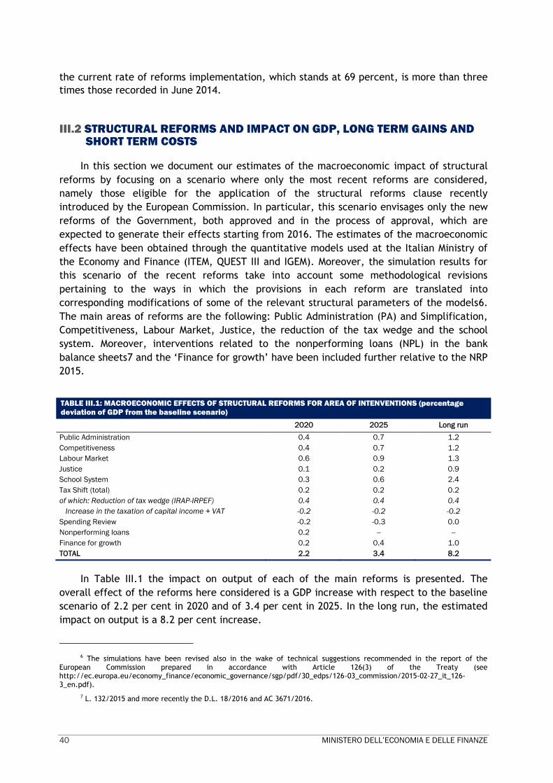
40 MINISTERO DELL’ECONOMIA E DELLE FINANZE
the current rate of reforms implementation, which stands at 69 percent, is more than three
times those recorded in June 2014.
III.2 STRUCTURAL REFORMS AND IMPACT ON GDP, LONG TERM GAINS AND SHORT TERM COSTS
In this section we document our estimates of the macroeconomic impact of structural
reforms by focusing on a scenario where only the most recent reforms are considered,
namely those eligible for the application of the structural reforms clause recently
introduced by the European Commission. In particular, this scenario envisages only the new
reforms of the Government, both approved and in the process of approval, which are
expected to generate their effects starting from 2016. The estimates of the macroeconomic
effects have been obtained through the quantitative models used at the Italian Ministry of
the Economy and Finance (ITEM, QUEST III and IGEM). Moreover, the simulation results for
this scenario of the recent reforms take into account some methodological revisions
pertaining to the ways in which the provisions in each reform are translated into
corresponding modifications of some of the relevant structural parameters of the models6.
The main areas of reforms are the following: Public Administration (PA) and Simplification,
Competitiveness, Labour Market, Justice, the reduction of the tax wedge and the school
system. Moreover, interventions related to the nonperforming loans (NPL) in the bank
balance sheets7 and the ‘Finance for growth’ have been included further relative to the NRP
2015.
TABLE III.1: MACROECONOMIC EFFECTS OF STRUCTURAL REFORMS FOR AREA OF INTENVENTIONS (percentage
deviation of GDP from the baseline scenario)
2020 2025 Long run
Public Administration 0.4 0.7 1.2
Competitiveness 0.4 0.7 1.2
Labour Market 0.6 0.9 1.3
Justice 0.1 0.2 0.9
School System 0.3 0.6 2.4
Tax Shift (total) 0.2 0.2 0.2
of which: Reduction of tax wedge (IRAP-IRPEF) 0.4 0.4 0.4
Increase in the taxation of capital income + VAT -0.2 -0.2 -0.2
Spending Review -0.2 -0.3 0.0
Nonperforming loans 0.2 -- --
Finance for growth 0.2 0.4 1.0
TOTAL 2.2 3.4 8.2
In Table III.1 the impact on output of each of the main reforms is presented. The
overall effect of the reforms here considered is a GDP increase with respect to the baseline
scenario of 2.2 per cent in 2020 and of 3.4 per cent in 2025. In the long run, the estimated
impact on output is a 8.2 per cent increase.
6 The simulations have been revised also in the wake of technical suggestions recommended in the report of the
European Commission prepared in accordance with Article 126(3) of the Treaty (see http://ec.europa.eu/economy_finance/economic_governance/sgp/pdf/30_edps/126-03_commission/2015-02-27_it_126-3_en.pdf).
7 L. 132/2015 and more recently the D.L. 18/2016 and AC 3671/2016.

MINISTERO DELL’ECONOMIA E DELLE FINANZE 41
Macroeconomic Impact of Finance for Growth measures
The economic crisis of recent years has exacerbated the problem of the credit crisis and, more
generally, the difficulties for companies in raising funds. Credit market rigidities represent a major
obstacle on the path of recovery and a strong limitation for investment and employment expansion. The
constraint is particularly burdensome for the peculiarities of the production structure of the country,
characterised by a large network of small and medium-sized enterprises, which represent the real
backbone of the Italian economy. In a context in which public resources tend to be scarce, it is crucial
to implement the effective incentives to improve the propensity to invest of private enterprises.
MEASURES RELATED LEGISLATION
Measures for innovation
Enlargement of the pool of innovative startup and
simplification measures
art. 4 of D.L. 3/2015 (Investment Compact)
Tax credit for R&D activities art. 3 of D.L. 145/2013, modified by art. 1,
subparagraphs 35 - 36 of Law 190/2014 (LDS2015) Patent box art. 1, subparagraphs 37 – 45 of Law. 190/2014 (LDS
2015) modified by art. 5, subpar. 1 of D.L. 3/2015
art. 1, subparagraph 148 Law 208/2015 (LDS2016)
PMI (SME) Innovative D.L. 3/2015 (Investment Compact) art. 4
Incentives for productive investments
Revision of New Sabatini art. 2 of D.L. 69/2013, Law 190/2014 (LDS2015), art.
1, subparagraph 243, D.L. 3/2015 Art. 8
Guidi – Padoan provision art. 18 D.L. 91/2014
Super amortisation art. 1, subparagraphs 1 91 -94 of Law 208/2015
(SL2016)
Access to capital market
Minibond art. 32 of D.L. 83/ 2012, (Decree for Development)
modified by art. 36, of D.L. 179/ 2012, (Decree for
Development bis) and by art. 12 of D.L.. 145/ 2013,
(Destinazione Italia), art. 21 of D.L.. 91/2014 Simplification measures for SMEs going public art. 20 of D.L. 91/2014
Introduction of multiple vote securities and loyalty shares
art. 20 of D.L. 91/2014
Development of Equity Crowdfunding art. 4 of D.L. 3/2015 (Investment Compact)
Measures for credit liberalisation
Direct lending for credit funds, insurance companies
and and securitization vehicles
art. 22 of D.L. 91/2014,
System of public guarantees, FCG, Confidi and Juncker investment platforms
Guarantee Fund for SME art. 8 - 8 bis of D.L. 3/2015
Juncker investment platforms Reg. (UE) 2015/1017, Art. 1, subparagraphs 822-830
of Law 208/2015 (LDS2016)
Incentives to capitalization
ACE art. 1. of D.L.. 201/2011 (Salva Italia), modified by art.
1, subparagraph 138 of Law 147/ 2013 (LDS2014)
and art. 19 of D.L. 91/2014 Deductibility of goodwill art. 1, subparagraphs 95 and 96 of Law 208/2015 (SL
2016)
Easier investment in infrastructure, real estate and project bonds
Revision of the legislation on project bond art. 1 of D.L. 83/2012 and art. 13 of D.L. 133/2014
Revision of the legislation on SIIQ (REIT) art. 20 D.L. 133/2014 (Sblocca Italia)
Measures to attract investments
International standard ruling art. 8 of D.L. 269/2003
Consulting services for foreign investors provided by
Agenzia delle Entrate (Revenue agency)
Provision of the Revenue Agency no. 149505 of 16
December 2013 (envisaged in D.L. 145/2013 art. 10
(Destinazione Italia) Court for companies with headquarter abroad
D.L. 145/2013 art. 10 (Destinazione Italia)
Increase of the threshold above which to notify the acquisition or disposal of major holdings
art. 20 of D.L. 91/ 2014 converted with modifications into L. 116/2014
FO
CU
S
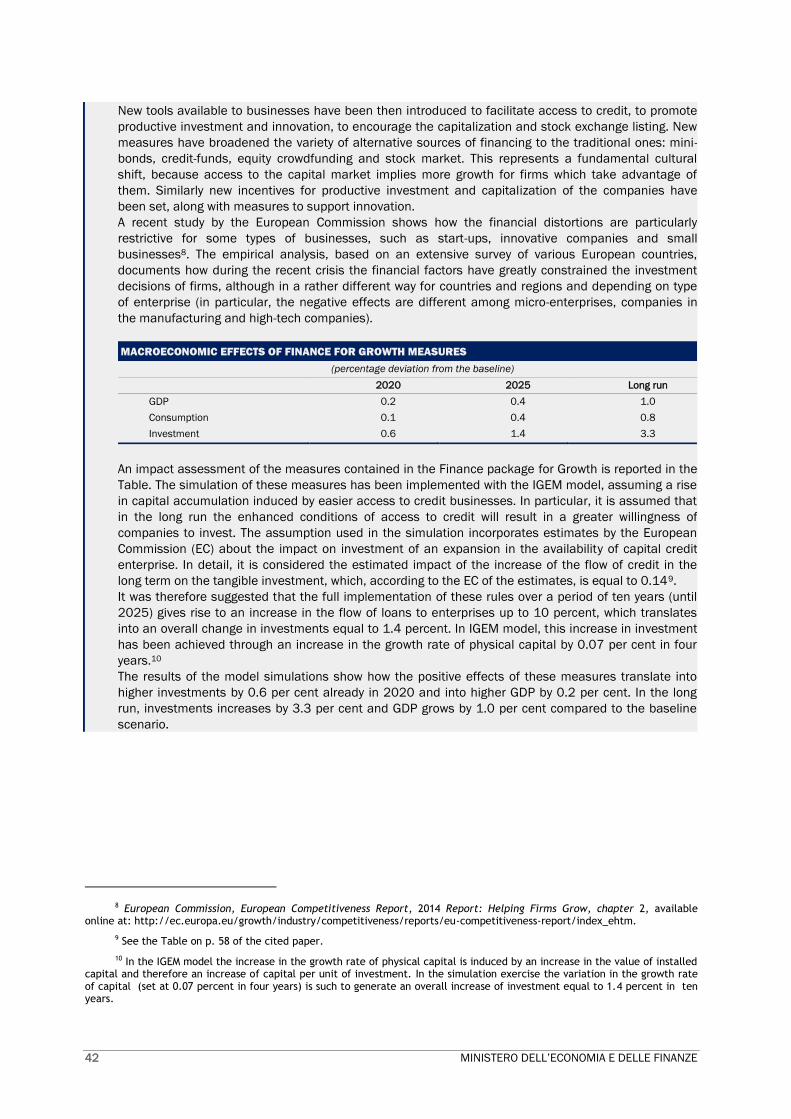
42 MINISTERO DELL’ECONOMIA E DELLE FINANZE
New tools available to businesses have been then introduced to facilitate access to credit, to promote
productive investment and innovation, to encourage the capitalization and stock exchange listing. New
measures have broadened the variety of alternative sources of financing to the traditional ones: mini-
bonds, credit-funds, equity crowdfunding and stock market. This represents a fundamental cultural
shift, because access to the capital market implies more growth for firms which take advantage of
them. Similarly new incentives for productive investment and capitalization of the companies have
been set, along with measures to support innovation.
A recent study by the European Commission shows how the financial distortions are particularly
restrictive for some types of businesses, such as start-ups, innovative companies and small
businesses8. The empirical analysis, based on an extensive survey of various European countries,
documents how during the recent crisis the financial factors have greatly constrained the investment
decisions of firms, although in a rather different way for countries and regions and depending on type
of enterprise (in particular, the negative effects are different among micro-enterprises, companies in
the manufacturing and high-tech companies).
MACROECONOMIC EFFECTS OF FINANCE FOR GROWTH MEASURES
(percentage deviation from the baseline)
2020 2025 Long run
GDP 0.2 0.4 1.0
Consumption 0.1 0.4 0.8
Investment 0.6 1.4 3.3
An impact assessment of the measures contained in the Finance package for Growth is reported in the
Table. The simulation of these measures has been implemented with the IGEM model, assuming a rise
in capital accumulation induced by easier access to credit businesses. In particular, it is assumed that
in the long run the enhanced conditions of access to credit will result in a greater willingness of
companies to invest. The assumption used in the simulation incorporates estimates by the European
Commission (EC) about the impact on investment of an expansion in the availability of capital credit
enterprise. In detail, it is considered the estimated impact of the increase of the flow of credit in the
long term on the tangible investment, which, according to the EC of the estimates, is equal to 0.149.
It was therefore suggested that the full implementation of these rules over a period of ten years (until
2025) gives rise to an increase in the flow of loans to enterprises up to 10 percent, which translates
into an overall change in investments equal to 1.4 percent. In IGEM model, this increase in investment
has been achieved through an increase in the growth rate of physical capital by 0.07 per cent in four
years.10 The results of the model simulations show how the positive effects of these measures translate into
higher investments by 0.6 per cent already in 2020 and into higher GDP by 0.2 per cent. In the long
run, investments increases by 3.3 per cent and GDP grows by 1.0 per cent compared to the baseline
scenario.
8 European Commission, European Competitiveness Report, 2014 Report: Helping Firms Grow, chapter 2, available
online at: http://ec.europa.eu/growth/industry/competitiveness/reports/eu-competitiveness-report/index_ehtm.
9 See the Table on p. 58 of the cited paper.
10 In the IGEM model the increase in the growth rate of physical capital is induced by an increase in the value of installed capital and therefore an increase of capital per unit of investment. In the simulation exercise the variation in the growth rate of capital (set at 0.07 percent in four years) is such to generate an overall increase of investment equal to 1.4 percent in ten years.

MINISTERO DELL’ECONOMIA E DELLE FINANZE 43
The macroeconomic effects of the reforms for reducing nonperforming loans (NPL) in the bank balance sheets In this note we document the macroeconomic effects of three Government measures adopted between
2015 and 2016 with the aim of reducing the stock of nonperforming loans (NPL) in the bank balance
sheets (D.L. 18/201611) and increasing the speed and efficiency of the insolvency and liquidation
procedures (D.L. 83/201512 and AC 3671/201613).
The first measure envisages the possibility of providing a State guarantee to banks for securitization
operations with nonperforming loans as the underlying assets (GACS). The State guarantees on NPLs
can be requested by banks which securitize in return for a commission to be paid to the Treasury
whose amount is a percentage on the guaranteed assets. The price of the guarantee is in line with
market prices. This provision is temporary, as the opportunity of requesting state guarantees in the
securitizations of NPLs has been introduced over a 18-month period, with the possibility, however, of
extending the application of the provision for other 18 months (until February 2019).
The other two measures are aimed at reforming the legislative tools for managing the company crises,
on the one side, and at reforming the bankruptcy, civil and civil procedure legislation as well as the
functioning of the judicial system, on the other. In particular, important provisions have been
introduced to reduce the foreclosure times and the length of the insolvency and liquidation procedures.
This enhances the efficiency of the judicial procedures for debt recovery, thus increasing the prices that
investors are willing to pay for the NPLs.
The macroeconomic effects of the first decree, the one on the bankruptcy legislation aimed at
accelerating the liquidation procedures, have already been documented in the Draft Budgetary Plan
(DBP) and they are now amplified as a result of the recent draft Law delegating the Government to
pursue further reforms on this area. In the simulation exercise with the ITEM model to assess these
effects, we assumed that those reforms would induce an increased incidence of disposed
nonperforming loans and a parallel reduction of the gap between book values on bank balance sheets
and the price that investors are willing to pay (pricing gap). This was implemented in the simulation of
the model through a gradual reduction of the discount that investors require for purchasing the
nonperforming loans.
In addition to the effects from the measures in the first decree, the new provision introducing a state
guarantee on securitization operations for NPL’s is likely to amplify the incidence of disposed
nonperforming loans. In particular, the assumption in the simulation associated with the first decree
was an increase in the amount of disposed NPLs as a fraction of its overall stock (in net value) by 10
percentage points (from 5 to 15 per cent). In light of the new provisions of 2016, the increase in the
incidence of disposed NPLs is assumed to be more pronounced, reaching 30 per cent in 2019.
Moreover, the higher easiness in disposing NPLs and reducing their burden in banks’ balance sheets,
combined with the interventions on bankruptcy law to accelerate the judicial procedures for debt
recovery, may induce banks to ameliorate the cost of lending. In the simulation we therefore assumed
a reduction by 10 basis point of the bank lending rate with respect to the baseline scenario up to 2019.
The improvement in the banks’ financial conditions due to the increased incidence of disposed NPLs
has a positive impact on the credit supply to the economy. This increase, combined with the slight drop
of the bank lending rate, would imply an increase of output with respect to the baseline scenario
reaching 0.2 percentage points in 2020, driven by higher investment (0.7 per cent) and consumption
expenditure (0.2 per cent). A possible reduction of credit, however, might be obtained in the first year of
simulation (2016) with respect to the baseline scenario, as a negative effect on loans is induced by the
reduction of total assets following the realized losses associated with the larger number of disposals of
nonperforming loans. The impact on GDP would be therefore slightly negative in the first year, with a
0.1 per cent reduction with respect to the baseline scenario, driven primarily by a drop of investment by
0.4 per cent. In the subsequent years, on the contrary, the expansionary effects on credit supply and
output would prevail. Given the temporary nature of the mechanism for providing state guarantee to
banks in the securitization operations, the simulation exercise does not extend its focus beyond 2020.
11 It is in the process of being converted into law.
12 Converted with modifications into L. 6, August 2015, no. 132).
13 Draft law (DDL) delegating the Government on the overall reform of the legislative tools to manage company crises and insolvency procedures. It has been approved by the Council of Ministers in February 10th 2016 and is currently under approval at the Chamber of Deputies (A.C. 3671).
FO
CU
S
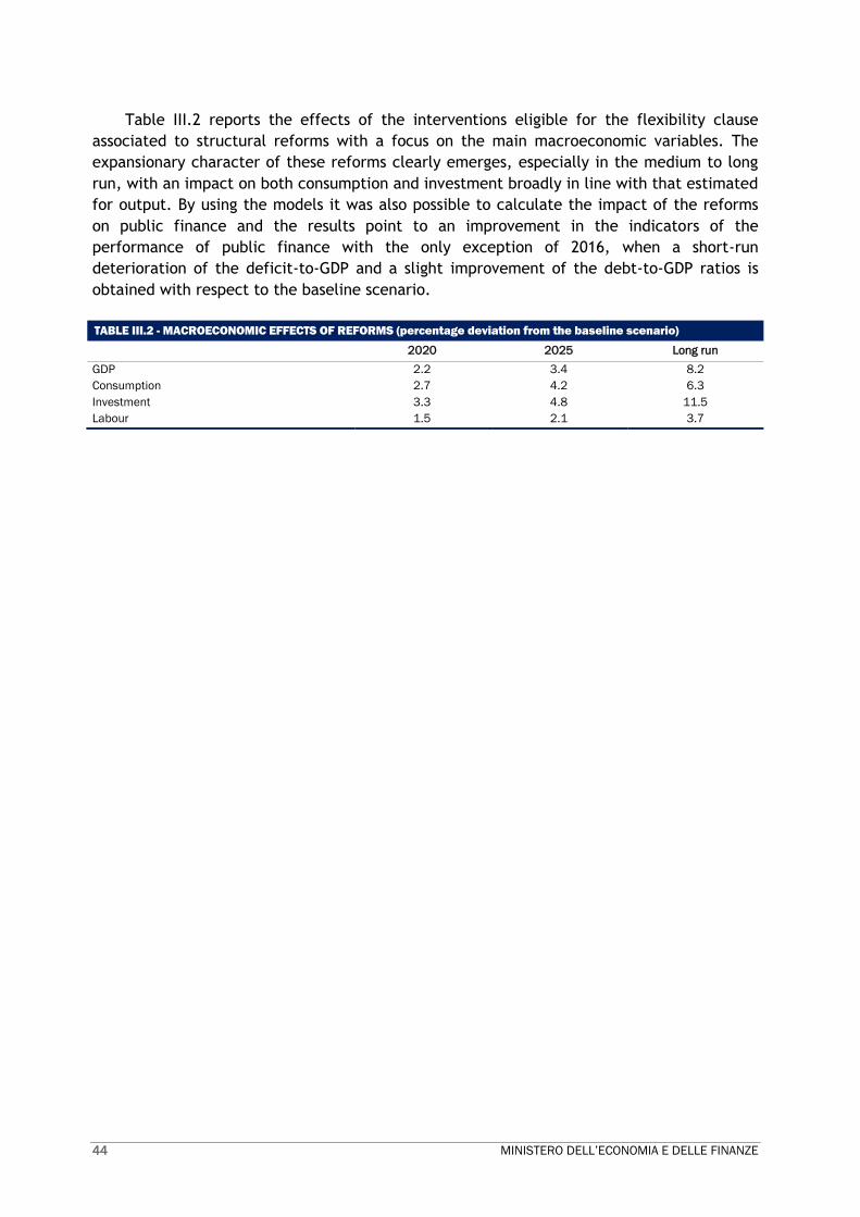
44 MINISTERO DELL’ECONOMIA E DELLE FINANZE
Table III.2 reports the effects of the interventions eligible for the flexibility clause
associated to structural reforms with a focus on the main macroeconomic variables. The
expansionary character of these reforms clearly emerges, especially in the medium to long
run, with an impact on both consumption and investment broadly in line with that estimated
for output. By using the models it was also possible to calculate the impact of the reforms
on public finance and the results point to an improvement in the indicators of the
performance of public finance with the only exception of 2016, when a short-run
deterioration of the deficit-to-GDP and a slight improvement of the debt-to-GDP ratios is
obtained with respect to the baseline scenario.
TABLE III.2 - MACROECONOMIC EFFECTS OF REFORMS (percentage deviation from the baseline scenario)
2020 2025 Long run
GDP 2.2 3.4 8.2
Consumption 2.7 4.2 6.3
Investment 3.3 4.8 11.5
Labour 1.5 2.1 3.7

MINISTERO DELL’ECONOMIA E DELLE FINANZE 45
IV. MEDIUM TERM BUDGETARY POSITION
IV.1 STRUCTURAL DEFICIT, FISCAL CONSOLIDATION AND CONVERGENCE TO THE MTO
During the period 2012-2014, in the midst of the most acute phase of the recession and
exceptionally bad cyclical conditions, Italy stayed the course of pursuing the Medium-Term
Objective (MTO) of a balanced budget in structural terms. No significant deviations with
respect to the requirements of the preventive arm of the SGP emerged.
Compliance with the requirements of the preventive arm of the Stability and Growth
Pact has also been assured in 2015 and in 2016 (see Table IV.1).
For 2015, both the Italian Stability Program and the 2016 Spring Forecasts show that the
structural balance has been reduced in line with the required effort over the single year and
over the average of two years (2014-2015). As for the expenditure rule, the national
projection points to a deviation of 0.4 percentage points of GDP in 2015 which, however, is
not significant and is not recorded by Commission services estimates (which, instead,
registered an over-achievement of the targeted adjustment equal to 0.13 percentage points
of GDP).
In 2016, the Italian Government applied for full application of the budget flexibility
allowed by the Preventive arm of the Stability and Growth Pact. Taking into account the
flexibility foreseen by the Structural Reforms clause and the one for co-financed
investments, the required fiscal effort would translate into a deviation of 0.25 percentage
points of GDP from the path of convergence to the MTO.
Vis-à-vis the allowed deviation of 0.25 percentage points, a deterioration of the
structural deficit of 0.7 percentage points of GDP recorded in 2016 in both in the Stability
Program and in the Spring Forecast would not be significant. In addition, the expenditure
aggregate is expected to grow, in real terms, by 0.5 per cent according to national
authorities and by 0.4 per cent according Commission services, in line with the respective
benchmarks. On the basis of such results, no significant deviation on the path of
convergence to the MTO would be recorded in 2016.
For 2017, under a no-policy-change assumption, the projections of the 2016 Spring
Forecast highlight a risk of significant deviation on both the structural balance criterion and
the expenditure rule both on the annual and on the two-year average. By contrast,
according to the policy scenario underlying the 2016 Stability program, there would be a risk
of significant deviation only for what concerns the structural balance. On the basis of the
measures that the Government is considering for 2017 the expenditure aggregate would post
a reduction of 0.5 per cent in real terms. As such, the deviation from the corresponding
benchmark would not be significant.
It is worth noting that under the Preventive arm of the SGP compliance with required
fiscal efforts is highly dependent on the way cyclical conditions are assessed through output
gaps and potential output calculations. On the basis of output gap estimates produced by
both the national authorities and Commission services through the commonly agreed
production function methodology, Italy would qualify as being in bad times in 2016 and in
46 MINISTERO DELL’ECONOMIA E DELLE FINANZE
normal times in 2017 — according to the matrix that specifies the structural required
adjustment1. As was argued above, the commonly agreed production function methodology
performs poorly with the NAWRU and TFP estimation for Italy, producing output gaps that
close fast and persistently low or negative potential growth due to counterintuitive negative
TFP trend contributions2.
To take into account such underlying uncertainty, compliance with the requirements of
the preventive arm of the SGP has been reassessed by re-calculating output gaps and
potential output estimates of the 2016 Spring Forecasts through the use of the enhanced
production function model presented earlier in this report. On the basis of the enhanced
methodology, Italian economy would indeed experience exceptional bad times in 2014 and
2015 (with output gaps being wider than -4.0 per cent of potential output), very bad times
in 2016 (with output gap being equal to -3.4 per cent) and bad times in 2017 (with output
gap being equal to -2.4 per cent of potential output).
The assessment of the significant deviation through the alternative potential output
estimates would yield a totally different picture (see Table IV.1). Up to 2016 compliance
with both the structural balance criterion and the expenditure rule would be ensured. In
2017, only a low risk of deviation would be signaled, as the annual deviation from the
required change in the structural balance would amount to -0.4 percent of GDP, and the
annual deviation of the expenditure aggregate would amount to -0.46 percent of GDP.
1 For 2016, the output gap is estimated at -2.3 per cent of potential output in Italy’s Stability Programme and at -1.6 per
cent in the Commission Services Spring Forecast. Output gaps higher than -3,0 per cent and lower than -1.5 per cent of potential output signal a situation of bad cyclicla conditions according to the Commission matrix specifying the required fiscal adjustment. For 2017, the output gap is estimated at -1.1 per cent of potential output in Italy’s Stability Programme and at -0.4 per cent in the Commission Services Spring Forecasts, signalling “normal” cyclical conditions.
2 TFP trends contribution to potential growth is estimated as being negative in Commission Services Forecasts since 2002 and until 2017.

MINISTERO DELL’ECONOMIA E DELLE FINANZE 47
TABLE IV.1: COMPLIANCE WITH THE PREVENTIVE ARM AND SIGNIFICANT DEVIATIONS
Structural balance criterion DEF 16
policy change scenario SF2016
SF2016 alternative model
on potential output
2014 2015 2016 2017 2014 2015 2016 2017 2014 2015 2016 2017
General Government deficit
(% of GDP)
-3.0 -2.6 -2.35 -1.8
-3.0 -2.6 -2.4 -1.9
-3.0 -2.6 -2.4 -1.9
Medium Term Objective
0.00 0.00 0.00 0.00
0.00 0.00 0.00 0.00
0.00 0.00 0.00 0.00
Structural deficit (% of GDP)
-0.81 -0.57 -1.23 -1.15
-1.14 -0.99 -1.65 -1.69
-0.39 -0.13 -0.66 -0.57
A=change in the structural deficit
-0.09 0.24 -0.66 0.08
-0.09 0.15 -0.66 -0.04
-0.09 0.26 -0.53 0.10
B=required change in the
structural deficit
0.00 0.25 -0.25 0.60
0.00 0.22 -0.25 0.60
0.00 -0.03 -0.50 0.50
C=A-B (no more than -0.5 pp)
Annual deviation from the required
change in the structural balance
-0.09 -0.01 -0.41 -0.52
-0.09 -0.07 -0.41 -0.64
-0.09 0.29 -0.03 -0.40
D=Two-year average change in the
structural balance
0.25 0.07 -0.21 -0.29
0.25 0.03 -0.26 -0.35
0.25 0.08 -0.14 -0.22
E=Required Two-year average
change in the structural balance
0.00 0.13 0.00 0.18
0.00 0.11 -0.02 0.18
0.00 -0.02 -0.27 0.00
F= D-E (no more than -0.25 pp)
Deviation of the two-year average
change in the structural balance
from the required values
0.25 -0.05 -0.21 -0.46
0.25 -0.08 -0.24 -0.53
0.25 0.10 0.13 -0.22
Expenditure Rule
DEF 16 policy change scenario
SF2016
SF2016 alternative model on potential output
2014 2015 2016 2017 2014 2015 2016 2017 2014 2015 2016 2017
A= Annual growth rate in the
reference expenditure aggregate
(%, in real terms)
-1.51 0.36 0.57 -0.46
-1.03 -0.75 0.35 0.21
-1.06 -0.74 0.35 0.20
B= Benchmark (modulated over
the prevailing cyclical condition +
flexibility clauses) (%)
0.04 -0.52 0.59 -1.30
0.04 -0.45 0.59 -1.36
0.04 0.10 1.14 -0.85
C= (no more than -0.5 pp) Annual
deviation of the expenditure
aggregate from the reference
determined by the benchmark (%
of GDP)
0.20 -0.40 0.01 -0.37
0.20 0.13 0.11 -0.70
0.20 0.38 0.36 -0.46
D= (no more than -0.25 pp ) Two-
year deviation of the expenditure
aggregate from the reference
determined by the benchmark (%
of GDP)
0.77 -0.10 -0.19 -0.18
0.77 0.17 0.12 -0.29
0.77 0.29 0.37 -0.05
Source: Own elaborations on DEF 2016 and on 2016 Spring Forecasts
IV.2 ITALY’S TRACK RECORD ON PRIMARY BALANCE, DEVELOPMENTS IN PRIMARY SPENDING AND QUALITY OF PUBLIC FINANCES
Since 2012, Italy’s headline deficit has been equal to or below 3 percent in spite of very
unfavorable cyclical conditions. It declined to 2.6 percent in 2015 and is projected to
further decrease in 2017 and beyond. The decline in net borrowing was ensured by the
maintenance of positive primary balances, which are among the highest recorded and
expected in the Euro Area (EA) and the European Union (EU).

48 MINISTERO DELL’ECONOMIA E DELLE FINANZE
According to data notified to EUROSTAT at the end of March 2016, in 2015 the primary
surplus was equivalent to 1.6 per cent of GDP (€26.1 billion). Italy’s ratio between the
primary surplus and GDP for 2015 was second only to that for Cyprus (2.2 per cent of GDP)
and Germany (2.1 per cent of GDP). The primary balance of other European partners with a
high public debt was equal to zero or in deficit last year. As a result, in 2015 the primary
surplus of the Euro Area amounted to 0.3 per cent of GDP, while the European Union had a
primary deficit of -0.1 per cent.
FIGURE IV.1 – GENERAL GOVERNMENT PRIMARY BALANCE, EDP (AVERAGE 2009-2015)
2016 European Commission Spring Forecast.
The impressive results in terms of the primary surplus are evident also in preceding
years. Italy’s primary surpluses have been on average the second largest in the EA and EU
during the 2009-2015 period3.
The 2016 European Commission Spring Forecast projects the Italian primary surplus at
1.6 per cent of GDP in 2016 and 1.9 per cent in 2017. The forecast for 2017 is above those
indicated in the 2016 Italy’s Stability Program based on the policy scenario (1.7 per cent of
GDP) and the current legislation (1.7 per cent of GDP). These trends confirm the soundness
of Italy’s primary balance position vis-à-vis the other European partners with a similar level
of debt-to GDP ratio and economic growth perspectives in the following two-years.
3 2016 European Commission Spring Forecast.
-8
-7
-6
-5
-4
-3
-2
-1
0
1
2
IE ES EL UK SI PT SK LT FR CY RO HR PL LV NL EU BG CZ EA FI BE AT DK EE SE MT HU LU IT DE
% o
f G
DP

MINISTERO DELL’ECONOMIA E DELLE FINANZE 49
FIGURE IV.2 – GENERAL GOVERNMENT PRIMARY BALANCE FORECAST, EDP (AVERAGE 2016-2017)
2016 European Commission Spring Forecast.
Thanks to the sustained primary surplus, the debt-to-GDP ratio has been broadly
stabilized in 2015. Based on projections of Italy’s 2016 Stability Program, the debt-to-GDP
ratio will decline in 2016 for the first time in eight years.
The maintenance of primary surplus has been accompanied by an ongoing improvement
in the composition of primary spending. In 2015, general government primary spending
declined to 46.3 per cent of GDP; primary current expenditure to 42.2 per cent of GDP,
while capital expenditure raised by 10.7 per cent in nominal terms year on year, reaching
the 4.1 per cent of GDP.
In 2015, public consumption continued to decline in absolute terms, falling to 19.0 per
cent of GDP, a level below the EA average (20.8 per cent of GDP). The reduction of
employee compensation, which fell by 1.1 per cent in nominal terms, and the slightly
positive dynamic of intermediate consumption reflect the measures affecting turnover, the
continuing freeze on contract renewals and the impact of the spending-review. Opposite to
these trends, gross fixed investment increased by 1.0 per cent over 2014, to 2.3 per cent of
GDP, after years of gradually declining.
Differently from the development observed on average in the Euro Area and in the EU
aggregates, as well as in the main European partners, Italy’s primary current spending would
have reduced in absolute terms in 2015 if the €80 fiscal bonus, which was introduced in 2014
and made permanent in 2015, had been classified as a lower tax rather than a social
transfer in cash.
-2
-1,5
-1
-0,5
0
0,5
1
1,5
2
2,5
FR RO FI PL DK ES BG UK SK NL EE SE LV BE EU CZ EA SI LT AT LU HU HR EL MT DE IT IE PT CY
% o
f G
DP

50 MINISTERO DELL’ECONOMIA E DELLE FINANZE
FIGURE IV.3 – GENERAL GOVERNMENT PRIMARY CURRENT SPENDING (LEVEL, 2010= 100)
* 2014 and 2015 data net of €80 bonus. Source: Elaboration on 2016 European Commission Spring Forecast.
According to the 2016 European Commission Spring forecasts, Italy’s public consumption
will continue to decline, reaching a level of 18.3 per cent of GDP in 2017, which is still
below the Euro Area and EU averages. A similar projection is indicated in the 2016 Italy’s
Stability Program (18.1 per cent of GDP at current legislation). Public investment is
expected to increase according to both the European Commission (by 0.9 per cent in 2016
and 0.6 per cent in 2017) and Italy’s official estimates. The implementation of the
Investment plan, for which Italy requested last autumn the additional budgetary flexibility
foreseen by the Stability and Growth Pact, will support also private investment and
positively impact potential growth.
The Commission should also consider the measures introduced in the latest years aiming
at minimizing the distortionary impact on economic growth on the revenue side: €80 euro
bonus; social contributions exemptions; reinforcement of ACE; labour-cost exemption from
IRAP tax base. At the same time, VAT rates and the taxation investment income have been
increased. Finally, the Revenue Agency’s strategy has been broadened to include forms of
spontaneous tax compliance on the part of taxpayers. From January 2017, the Corporate
Income Tax rate will be lowered from 27.5 to 24.5 per cent.
Finally, special consideration should be given to the recent institutional improvement
directed to improve the management of public resources and the budget process, which will
help ensure compliance with national fiscal rules, especially the spending benchmark.
First, the recent reforms put forth by the government will enhance the budget process.
According to the new regulation: i) expenditure targets are set for each Ministry by the end
of May; ii) the Ministries should then propose efficiency improvements in the use of
resources through administrative procedures and any regulatory proposals designed to
achieve the expected results/spending ceiling; iii) these proposals are evaluated for the
purpose of their inclusion in the Stability Law and subject to parliamentary debate during
the approval process of the budget. The decrees also streamline the classification of the
90
95
100
105
110
115
2010 2011 2012 2013 2014 2015
PT
ES
IT (*)
EA
EU
DE
FR

MINISTERO DELL’ECONOMIA E DELLE FINANZE 51
State budget, in order to make it easier to read, by linking underlying policies to services
being provided.
Second, as for tax expenditures, the reform envisages the preparation of a specific
annual report on tax allowances. This report will be the basis for the revision of tax
expenditures to be made operational in the budget (Stability Law).
To sum up, the provision of Regulation 1467/97 states that the Commission, when
preparing a report under Article 126 (3), should consider: i) the level of the primary
balance, ii) the development in primary expenditure, both current and capital; iii) the
overall quality of public finances, in particular the effectiveness of national budgetary
frameworks.
The Government is firmly convinced that the aforementioned elements should be
considered as relevant factors for assessing Italy’s medium term budgetary position.

52 MINISTERO DELL’ECONOMIA E DELLE FINANZE

MINISTERO DELL’ECONOMIA E DELLE FINANZE 53
V. DEVELOPMENTS IN THE GOVERNMENT DEBT POSITION
V.1 DEVELOPMENTS IN GOVERNMENT DEBT POSITION
According to the 2016 Commission services Spring Forecast, Italian public debt as a
ratio of GDP has increased, on average, by more than 5.0 percentage points over 2012-2014,
but the rate of growth is expected to slowdown in 2015 and to halt in 2016. In 2017, under
the no-policy change assumption, debt/GDP ratio is expected to reduce by 1,0 percentage
points of GDP.
Over 2012-2014, the increase in Italian debt has been the result of factors that are
mostly outside the direct control of national authorities. These are, in terms of relevance:
the piling up effects coming from interests; the impact negative of real GDP growth; and the
negative contribution coming from the stock-flow adjustment. The snowball effect has also
been amplified in the current environment of low inflation.
Overall, the snowball effect has raised debt, on average, by 5.5 percentage points of
GDP. Among its underlying components, the lion share has been represented by the impact
of interest expenditure. However, a sizeable portion of this increase has to be accounted for
the effect of negative real GDP growth experienced in 2012-2014, which pushed the debt-to-
GDP ratio up, on average, by 2.0 percentage points.
By contrast, the counterbalancing impact coming from inflation (i.e. growth in GDP
deflator) has been extensively subdued. Indeed, with an average change in GDP deflator
equal to 1.1 per cent, the reducing impact on public debt has been, on average, around 1.4
percentage points of GDP. In this respect, it is worth highlighting that, due to the underlying
low-flationary dynamics prevailing over 2014 and expected for 2015, the debt reducing
impact stemming from prices is expected to shrink further.
Against this backdrop, in spite of the difficult cyclical conditions, Italian governments
have been able to run significant primary surpluses over the 2012-2014 period amounting, on
average, to 1.9 per cent of GDP, a figure which is well above the historical average primary
surplus recorded since 2001, equal to 1.4 per cent of GDP. By contrast, the contribution
coming from the Stock Flow Adjustment has pushed the debt-to-GDP ratio up by, on
average, almost 1.8 percentage points, completely offsetting the reduction effect stemming
from the budgetary tightening.
In 2015, thanks to the high primary surplus projected both by the latest Commission and
the Italian government estimates and thanks to the real output recovery, the debt-to-GDP
has increased only 0.2 percentage points in spite of the lacklustre price developments. The
piling up impact coming from the snowball effect has remained significant and prevailing
but it has been almost offset by the countervailing contributions stemming from primary
surplus and stock flow adjustment components, with the latter benefitting from substantial
yields from privatisations.
In 2016, the debt-to-GDP ratio is expected to stabilize according to Commission
estimates. The impact of the snow-ball effect will be reduced thanks to higher real GDP
growth and completely offset by the declining contribution of primary surplus.

54 MINISTERO DELL’ECONOMIA E DELLE FINANZE
In 2017, under a no-policy change assumption, debt/GDP ratio is expected to diminish
by 1,0 percentage points thanks to the increase in the primary surplus and a more
substantial contribution coming from real growth and price dynamics.
Figure V.1 compares the change in debt-to-GDP ratio occurred in Italy between 2012
and 2017 to the Euro Area aggregate, isolating the impact of each underlying component.
In 2015, the debt/GDP ratio has been decreasing in the Euro Area thanks to the
contribution coming from real GDP growth and inflation which, instead, lacked in Italy. In
addition, differently from the Italian case, the primary balance has not contributued to the
debt reduction in the Euro Area.
FIGURE V.1 - ANNUAL CHANGE IN THE GROSS DEBT RATIO, BASELINE SCENARIO (2016 Spring Forecast)
ITALY
EURO AREA
Source: European Commission, Spring Forecast 2016
-6,0
-4,0
-2,0
0,0
2,0
4,0
6,0
8,0
10,0
12,0
2012 2013 2014 2015 2016 2017
p.p
. o
f G
DP
Stock-Flow Adjustment (SFA) Real growth effect
Inflation effect Interest rate
Primary balance ( +=deficit) Yearly change in debt-to-GDP
-6,0
-4,0
-2,0
0,0
2,0
4,0
6,0
8,0
2012 2013 2014 2015 2016 2017
p.p
. o
f G
DP
Stock-Flow Adjustment (SFA) Real growth rate
Inflation (GDP deflator) Interest rate
Primary balance ( +=deficit) Yearly change in debt-to-GDP

MINISTERO DELL’ECONOMIA E DELLE FINANZE 55
V.2 IMPACT OF QE ON THE DEBT/GDP RATIO
In January 2015 the ECB officially announced the start of its QE program (called PSPP,
Public Sector Purchase Program) for the following March. The programme envisaged the
purchase of all tgovernment bonds with a residual maturity above 2 years and below 30
years, for a total monthly volume of 60 billion at the euro area level. From March 2015 up
to December 2015 the ECB, through the National Central Bank, has bought around 71 billion
of Italian government bonds in market value terms, corresponding to an average of 7 billion
per month. Following the same trend in the first quarter of 2016 the total volume reached
95 billion euros. In March 2010 the ECB announced the extension in time and size of the
purchase program: it will last up until March 2017 for a monthy volume of 80 billion euro:
for Italy this meant an increase of public bond purchases of around 3 billion per month on a
market value terms.
The initiative of the ECB has of course brought a significant reduction of interest rates
on Italian government paper: in 2015 the 2 year maturity went down from 0.5 per cent to
0.04 per cent, the 10 year maturity from 1.75 per cent to 1.40 per cent. However, a
significant drop in interest rates took place even before the official announcement, as the
QE was widely in line with market expectations.Indeed in November 2014 the Italian 2-year
rate was 0.70 per cent while the 10 year rate was hovering around 2.35 per cent showing
therefore that a remarkable reduction had already taken place before the ECB’s
announcement. Thanks to this reduction in market rates the Treasury was indeed able to
significantly reduce the cost at issuance of new debt. In 2015 this cost almost halved with
respect to 2014 moving down from 1.35 per cent to 0.70 per cent. However this was not
accompanied by a proportionate reduction in the average cost of debt that went down only
from 3.59 per cent to 3.20 per cent. This dynamic took place also before 2015: going
backward to the last decade, the evolution of the average cost has always been much less
volatile than that of the marginal cost.
During the last 20 years Italy has carried out significant efforts to reduce the debt
exposure to the interest rate risks by lengthening both the average life and the duration of
the stock of government securities outstanding (Figure V.2)and reinforce the evolution of
average refixing period (ARP) 1, anindex which quantifies the interest rate risk born by a
debt portfolio, which at the end of 2015 reached 5.42 years.
More specifically, give the current debt structure, it takes more than 5 years for a new
level of market rates to be incorporated by the whole Italian public debt. These results
have been achieved mainly with the issuance policy that over time was more heavily skewed
towards long term bonds, lightening the recourse to Treasury Bills, floating rate notes and
short bonds. The only period when this policy has slightly changed was during the sovereign
debt crisis as the market for long bonds was not big enough to absorb the same sizes of the
previous years.
1 The average refixing period reflects the average time still to elapse (without discounting the flows) before the debt
structure incorporates the new market rates. For real or nominal fixed-rate securities, the indicator is based on the residual life of each security, whereas for variable-rate securities, the indicator is based on the time to elapse until the indexing of the next coupon. Each security is included in the weighted calculation for the nominal value outstanding.

56 MINISTERO DELL’ECONOMIA E DELLE FINANZE
FIGURE V.2 – AVERAGE LIFE AND DURATION OF GOVERNMENT SECURITIES OUTSTANDING
Source: MEF simulations on 2016 Commission Services Spring Forecasts
These efforts have been significantly restored since the end of the sovereign debt crisis
in 2013 and even more since the QE started in order to offset the reduction that average life
and duration show during the sovereign debt crisis (2011-12).
The resulting outcome of such an issuance policy has been the significant reduction of
the total debt interest burden sensitivity to market shocks, something absolute crucial for a
large debt country in order to ring fence the fiscal consolidation process from potential
market turbulences.
TABLE V.1 – INTEREST EXPENDITURE SENSITIVITY TO MARKET SHOCKS
Interest sensitivity/GDP
Years DEF 2016 DEF 2015 DEF 2014
1st 0.13 0.15 0.17
2nd 0.28 0.29 0.34
3rd 0.40 0.40 0.44
4th 0.50 0.49 0.53
Source: MEF simulations on 2016 Commission Services Spring Forecasts.
Looking at Table V.1, currently a permanent shock of 100 basis points on the whole
yield curve has an impact on the interest debt burden of only 0,13 points of GDP over the
first year, compared with the one that could arise if the shock had to be incorporated
immediately by the whole stock of government securities, amounting to 1.13 per cent of
GDP with debt data as of end of 2015. Moreover the Table V.1 shows that this sensitivity
over the past few years, including the period discounting the effects of the ECB QE, has
continued to move down, highlighting the increasing resilience of the debt stock to market
shocks. Indeed the share of instruments with a maturity equal or above 10 years, over the
total issuance activity, has risen from around 16 per cent in 2014 to 20 per cent in 2015.
Looking at the only first quarter, this share increased from around 12 per cent in 2014 to 24
per cent in 2015. In the first quarter of 2016 the trend is fully confirmed at 24 per cent.
3,0
3,5
4,0
4,5
5,0
5,5
6,0
6,5
7,0
7,5
1999 2000 2001 2002 2003 2004 2005 2006 2007 2008 2009 2010 2011 2012 2013 2014 2015
Ye
ars
Average life Duration

MINISTERO DELL’ECONOMIA E DELLE FINANZE 57
The downside of this policy is that, symmetrically, with the current structure of debt it
takes also years for the drop in bond yields, like the one brought by the QE, to significantly
reduce the average cost of funding. Looking at Figure V.3 it is clear-cut that the increasing
difference in the speed of reduction of the two types of costs since the end of the sovereign
debt crisis in 2012, a period of dramatic drop of the whole Government yield curve.
FIGURE V.3 – COMPARING DEBT COSTS: MARGINAL VS AVERAGE
Source: MEF simulations on 2016 Commission Services Spring Forecasts.
In addition it must also be highlighted that the reduction of interest rates caused by the
QE has not been uniform across the government yield curve. Since January 2015 - when the
QE decision was announced - the slope of the yield curve – as measured by the spread
between the 1 year and the 10 year rate - has been higher than the level of January 2015 for
most of the period up to now.
Therefore, by issuing significantly more on longer maturities, in order to strengthen the
debt structure as described above, Italy has somehow given up further potential interest
burden reduction that could have contributed, at the margin, in lowering the current and
expected debt/GDP levels thereby fostering its reduction path. In a ceteris paribus context,
if one applies the reduction experienced in terms of cost-at-issuance from 2011 to 2015 to
the whole stock of government securities as of December 2010, the interest burden would
have dropped by 2.8 points of GDP on a cumulative basis over the four years. Focusing only
on the QE period, the reduction of cost-at-issuance from 2014 to 2015 would have brought
an interest burden decline of 0.7 points of GDP, if applied to the whole debt stock at the
end of 2013.
4,44 4,46
4,88 5,06
4,15
3,89
4,12 4,4
3,91 3,59
3,2
2,47
3,32
4,14 4,09
2,18 2,10
3,61
3,11
2,08
1,35
0,70
0
1
2
3
4
5
6
2005 2006 2007 2008 2009 2010 2011 2012 2013 2014 2015
%
Average debt cost Average cost at issuance

58 MINISTERO DELL’ECONOMIA E DELLE FINANZE
V.3 RISKS RELATED TO THE STRUCTURE OF PUBLIC DEBT FINANCING
Changes in the share of short-term public debt provide an indication of
increased/decreased vulnerability of the country under examination in terms of
government’s reliance on short term market financing. In the European Commission’s
approach, those values would be examined in relation to a set of calculated critical
thresholds of fiscal risks, according to the so called signals’ approach so as to establish
whether fiscal risks related to the structure of public debt financing may eventually emerge.
According to the Commission methodology for assessing debt sustainability, the yearly
change in share of short term public debt should be considered risky if higher than 2.2
percentage points or highly risky if higher than 2.76 percentage points. On the basis of
Eurostat figures, between 2013 and 2014, the share of short term debt of Italy has
decreased by 0.6 percentage points, well below the critical thresholds. According to data
recently published by the Bank of Italy2, during the year 2015 the share moved further down
by approximately 1.5 percentage points.
Italy’s public debt presents a maturity structure that compares favorably with those of
other developed countries, being among the highest in Europe. With reference to the stock
of government securities, which represents over 84 per cent of the total, Italy's debt
recorded in 2016 an average life of 6.55 years (end of April 2016) vis-à-vis an average
maturity for the G-20 aggregate of 6.7. In 2016, the debt-to-average maturity (i.e. an
indication of the amount of new issued bonds) will be 20.6 per cent of GDP, a value not far
from the average of 18.0 per cent for G20 advanced countries (Table V.2). Almost all of
Italy's debt is denominated in euros, making for no foreign exchange risk3.
2 Supplemento al Bollettino Statistico – Finanza pubblica, fabbisogno e debito n. 9 del 13 febbraio 2015. Tavola 8
3 At any rate, however, the Italian Treasury uses currency swaps to hedge against exchange rate risks when issuing in a foreign currency.

MINISTERO DELL’ECONOMIA E DELLE FINANZE 59
TABLE V.2 - STRUCTURAL INDICATORS FOR THE DEBT IN 2016
Country Average term to maturity, 2016 Debt-to-average maurity, 2016
AT 7.9 10.8
BE 8.0 13.4
DE 5.9 11.5
ES 6.1 16.2
FI 7.0 14.0
FR* 7.1 14.0
IT** 6.6 20.6
NL 6.3 10.5
PT 6.8 18.8
SI 6.3 12.7
SWE 4.9 8.8
UK 14.8 6.0
USA 5.7 18.9
JPN 7.2 34.6
AUS 6.8 5.8
CAN 5.4 17.2
G20 ADV. 6.7 18.0
Source: IMF Fiscal monitor - April 2016.
(*) Figures provided by national authorities.
(**) End of April 2016
In order to have a more comprehensive assessment of risks related to public debt
overall sustainability, information on explicit liabilities are integrated with information on
governments’ contingent liabilities, which are by nature potential and not actual.
The following Figures report latest statistics on government’s contingent liabilities,
including:
The overall value of government guarantees in percentage of GDP, as from data published by Eurostat;
Liabilities of governments controlled entities classified outside general government (public corporations).
FIGURE V.4 - TOTAL STOCK OF GOVERNMENT GUARANTEES IN % OF GDP, 2014
Source: Eurostat, Newsrelease nr. 20/2016.
0
5
10
15
20
25
30
SK CZ BG LT LV EE RO HR IT NL FR PL PT LU HU UK DK SE BE SI ES IE CY DE MT FI AT EL
% o
f G
DP

60 MINISTERO DELL’ECONOMIA E DELLE FINANZE
FIGURE V.5 - TOTAL LIABILITIES OF GOVERNMENT CONTROLLED ENTITIES IN % OF GDP, 2014
Source: Eurostat, Newsrelease nr. 20/2016.
In a comparison with main European partners, Italy has one of the lowest stocks of
guarantees in 2014: at 2.7 per cent of GDP. The highest levels have mainly referred to the
countries whose financial systems were hardest hit by the crisis, including Ireland, Austria,
Greece and Spain.
The further disaggregation (not showed in the Figure) shows that data on government’s
contingent liabilities in percentage of GDP are mostly related to public support to financial
institutions. In 2014, almost one-half of Italy’s guarantees referred to the banking system
(approximately 1.5 per cent of GDP against total 2.7 per cent).
According to the more recent data published in the 2016 Italy’s Stability Programme,
the guarantees granted by the Italian government amounted to approximately €36.8 billion
in 2015, or 2.3 per cent of GDP, with a reduction of €6.5 billion year on year. The
guarantees granted to credit institutions following the financial crisis declined to €6.4 billion
(0.4 per cent of GDP). Such a support has been significantly decreased over the last year (by
€17 billion), because many financial institutions having improved their capital ratios, have
asked for withdrawing. In particular, as far as the so-called "Monti Bonds" are concerned,
such guarantees - amounting to 4 billion of euro in 2013 - have been fully repaid last year by
the issuing bank (MPS).
Moreover, the potential risk stemming from the Italian government’s participation in
corporations’ capital are in line with the major economies of the European Union and below
figures of other countries with lower level of public debt.
V.4 PARTICIPATION IN EURO AREA SOLIDARITY PROGRAMMES, TRADE DEBT ARREARS AND PRIVATISATIONS
Italy is among the Member States providing funding to financial stability mechanisms set
at the European level since the onset of the sovereign debt crisis in 2011, though it has not
benefitted from any support. These transactions have exerted a significant impact on the
level of public debt.
0
20
40
60
80
100
120
140
SK CZ BG LT LV EE RO HR IT NL FR PL PT LU HU UK DK SE BE SI ES IE CY DE MT FI AT EL
% o
f G
DP

MINISTERO DELL’ECONOMIA E DELLE FINANZE 61
According to the figures published in the 2016 Economic and Financial Document, the
funding to financial stability mechanisms (ESM, EFSF) together with the financing of the
Greek programs amounts to about 0.8 per cent of GDP in 2011, 2.6 per cent of GDP in 2012,
3.5 per cent of GDP in 2013, 3.7 per cent of GDP in 2014 and 3.6 per cent of GDP 2015. In
2016-2019, the impact of such components is expected to be, on average, around 3.3 per
cent of GDP.
Were these loans excluded, under the policy scenario indicated in the 2016 Economic
and Financial Document, the debt-to-GDP ratio would be 128.8 per cent of GDP in 2014 and
about 129.1 per cent of GDP in 2015.
Moreover, in line with recommendations from the Commission - included, with specific
reference to the case of Italy, in the statement by Vice Presidents Rehn and Tajani on
commercial debt of public administrations on 18 March 2013 -, since 2013 the Italian
government has introduced legislative initiatives for the settlement of general government
overdue trade debts via an extraordinary liquidation plan. So far, about €57 billion were
allocated in 2013 and 2014 (of which €27.2 billion in 2013 and €29.8 billion in 2014). The
impact of these payments on the debt-to-GDP is 1.2 per cent of GDP in 2013, 2.2 per cent in
2014 and 2.5 per cent of GDP in 2015 and 2016. If the effects stemming from these
payments were excluded from the debt-to GDP ratio together with the EU contribution to
solidarity mechanisms, the ratio would be 124.2 per cent in 2013, 126.6 per cent of GDP in
2014 and 2015, and 126.4 per cent in 2016 under GDP forecast indicated in the 2016
Stability Programme.
Indeed, the statement reads as follows “While the existing EU framework for budgetary
surveillance does not envisage a special treatment for specific debt and deficit increasing
items, the Stability and Growth Pact allows taking into account relevant factors in the
assessment of compliance with the deficit and debt criteria. In this context, the liquidation
of overdue commercial debt would represent a mitigating factor”4.
Finally, the Italian government remains committed to the privatisation plan via the
listing and subsequent disposal of stakes in state-owned enterprises as well as property and
land. In 2015, privatization proceeds exceeded 0.4 per cent of GDP. The goal for the 2016-
2018 is to achieve revenues of 0.5 percent of GDP per annum. The 2016 plan includes the
sale of a stake in ENAV, the air traffic control operator. The state railways (Ferrovie dello
Stato) are also part of the medium-term privatization plan along with companies that are
already listed and where the government could be reducing its participation.
4 MEMO/13/231 - Statement by Vice Presidents Rehn and Tajani on commercial debt of public administrations. Brussels,
18 March 2013.

62 MINISTERO DELL’ECONOMIA E DELLE FINANZE

MINISTERO DELL’ECONOMIA E DELLE FINANZE 63
VI. DEBT SUSTAINABILITY
VI.1 MEDIUM TERM DEBT-TO-GDP PROJECTIONS
The development of Italian public debt over the medium term is assessed by considering
the 2015 Fiscal Sustainability Report1 (FSR) and the projections presented by national
authorities in the 2016 Stability Programme.
According to the 2016 Spring Forecasts, the debt-to-GDP ratio is projected to remain
stable between 2015 and 2016 at the level of 132.7 per cent, and starting to decrease in
2017 reaching 131.8 per cent of GDP. The European Commission Fiscal Sustainability Report,
which presents several projection scenarios over the next ten years, confirms and reinforces
such results.
More in details, in the so-called baseline scenario, which is based on a no policy change
assumption2, Italian public debt as a ratio of GDP is expected to fall at a rate of almost 2
per cent of GDP per year from the peak of 2015 to 110 per cent in 2026.
Similar decreasing pattern are evident in all the other simulation scenarios even in the
more pessimistic ones such as, for instance, the one assuming a permanent positive shock
(+2p.p./+1p.p) to the short- and long-term interest rates on newly issued and rolled over
debt. In this scenario, the debt/GDP ratio is expected to fall at a rate of almost 1 per cent
of GDP per year from the peak of 2015, reaching 120 per cent of GDP in 2026 (Figure VI.1).
In addition, based on the stochastic debt simulation analysis, according to Commission
estimates, the probability that Italian debt in 2020 is going to be higher than the 2015 peak
in the next 5 years is 11 per cent, the second lowest probability after that of Germany (3
per cent).
1 European Commission, 2015, Fiscal Sustainability Report, European Economy Institutional Paper n. 018, also available
at: http://ec.europa.eu/economy_finance/publications/eeip/pdf/ip018_en.pdf
2 The FSR deterministic debt-to-GDP projections are based on the Commission services 2016 Winter Forecasts up to 2017. From 2018 up to 2026, the no-policy change scenario is carried out assuming that the 2017 structural balance will be kept constant over the projection horizon, changing only to take into account the impact of age-related expenditures as projected in the 2015 Ageing Report. Potential output growth is assumed to evolve in line with country-specific paths derived on the basis of the T+10 production function extrapolation methodology agreed by the Output Gap Working Group (OGWG). Long-term interest rate converge to 3 per cent in real term at the end of the projections horizon. Inflation is measured trough the growth rate of GDP deflator which is assumed to converge to 2 per cent in 2020. The output gap closes linearly in 2020 starting from the level of 2017. The Stock-Flow adjustment is assumed equal to zero from 2018 onwards.
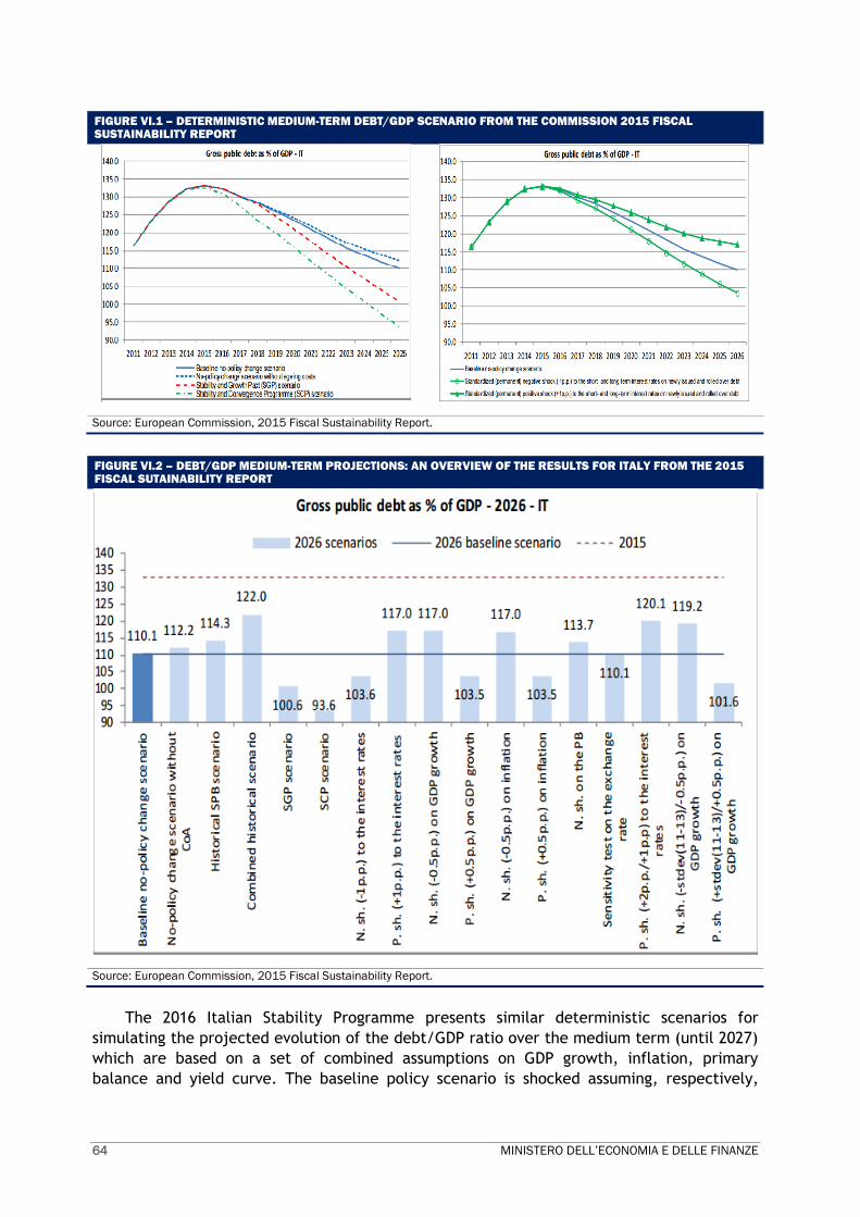
64 MINISTERO DELL’ECONOMIA E DELLE FINANZE
FIGURE VI.1 – DETERMINISTIC MEDIUM-TERM DEBT/GDP SCENARIO FROM THE COMMISSION 2015 FISCAL SUSTAINABILITY REPORT
Source: European Commission, 2015 Fiscal Sustainability Report.
FIGURE VI.2 – DEBT/GDP MEDIUM-TERM PROJECTIONS: AN OVERVIEW OF THE RESULTS FOR ITALY FROM THE 2015 FISCAL SUTAINABILITY REPORT
Source: European Commission, 2015 Fiscal Sustainability Report.
The 2016 Italian Stability Programme presents similar deterministic scenarios for
simulating the projected evolution of the debt/GDP ratio over the medium term (until 2027)
which are based on a set of combined assumptions on GDP growth, inflation, primary
balance and yield curve. The baseline policy scenario is shocked assuming, respectively,

MINISTERO DELL’ECONOMIA E DELLE FINANZE 65
higher/lower real GDP growth (+/- 0.5 per cent per year) over the period 2016-2019 coupled
with, respectively, lower/higher yield curve (-40 b.p in the optimistic scenario/+100 b.p in
the pessimistic one). In all of the scenarios, the projections of the debt-to-GDP ratio are
carried out by the endogenous estimation of the implicit interest rate which, in turn,
considers the assumptions about the trend of the yield curve and the assumptions about the
primary surplus. The alternative scenarios allow certain interactions between
macroeconomic variables so that, for example, lower growth rates are matched with lower
primary surpluses and with higher borrowing costs.
In addition, in order to test the sensitivity of the low growth scenario, to two additional
scenarios have been added. The first one simulates over the medium term (2027) the effect
on debt/GDP dynamic of a prolonged deflation caused by the failure of the QE. The second
scenario simulates the effect of a decoupling assumption according to which, thanks to a
mix of structural policies, Italy’s overall competitiveness increases but the level of the
prices, over the medium term, remains permanently below the European average, which
instead converges to the target of 2 per cent.
Table VI.1 illustrates in more detail the characteristics of the shocks applied to the
main macroeconomic and public-finance variables underlying the trend of the debt-to-GDP
ratio under the high/low growth scenarios and under the assumption of decoupling and
failure of the QE. Table VI.2 reports the values of the main macroeconomic and public-
finance variables of the different scenarios for the 2016-2019 period and the values of
convergence at the end of the medium-term forecast horizon.

66 MINISTERO DELL’ECONOMIA E DELLE FINANZE
TABLE VI.1: SUMMARY OF MACRO-FISCAL SHOCKS
HIGH/LOW GROWTH SCENARIOS: DESCRIPTION OF WORKING ASSUMPTIONS High growth Baseline LOW GROWTH
GDP a) +0.5 p.p. per year compared with the baseline projections in 2016-2019 period b) convergence from 2019 to 2027 to the pre-crisis value (2007) per NAWRU (7.8%) and pre-crisis average for TFP (0.5%)
a) EFD baseline scenario (2016-2019) b) convergence at structural parameters of the OGWG T+10 scenario
a) -0.5 p.p. per year compared with the baseline projections in 2016-2019 period b) convergence from 2019 to 2027 to average values of crisis years for NAWRU (10 %), and TFP (0.05%)
Yield curve a) yield curve equal to baseline scenario at start of 2018 (end of QE). Reduction of 40 bp through 2021 b) as of 2021, convergence at the values of the yield curve in the baseline scenario
a) Yield curve from EFD policy scenario (2015-2019) b) Constant yield curve as from 2019
a) +100 bp increase in yield curve in the 2016-2018 period b) in 2019, gradual convergence to the values of the yield curve in the baseline scenario
Primary surplus a) redetermination of primary surplus based on elasticity (sensitivity analysis) in the 2016-2019 period b) in 2020-2027, structural primary surplus constant at 2019 level
a) primary surplus as per EFD policy scenario (2016-2019) b) in 2020-2027, structural primary surplus constant at 2019 level
a) redetermination of primary surplus based on elasticity (sensitivity analysis) in the 2016-2019 period b) in 2020-2027, structural primary surplus constant at 2019 level
Inflation a) increase of deflator as per high-growth scenario in the years 2016-2019 b) convergence to 2% between 2019 and 2022
a) baseline scenario dal 2016-2019 b) convergence to 2% between 2019 and 2022
a) reduction of deflator as per low-growth scenario in the years 2016-2019 b) convergence to 2% between 2019 and 2022
DEFLATION SCENARIOS: DESCRIPTION OF WORKING ASSUMPTIONS
QE failure scenario Low-growth scenario Decoupling
versus Euro Area inflation and nominal devaluation
GDP a) -0.5 p.p. per year compared
with baseline projections for
2016-2019
a) -0.5 p.p. per year compared
with baseline projections for
2016-2019
a) -0.5 p.p. per year compared with
baseline projections for 2016-2019
b) convergence in 2019-2027 to
average values of the crisis for
NAWRU (10 %), and TFP (0.05%)
b) convergence in 2019-2027 to
average values of the crisis for
NAWRU (10%), and TFP (0.05%)
b) convergence to structural
parameters, such as OGWG T+10 in
baseline scenario Yield curve a) increase in yield curve (+100
bp) in the 2016-2018 period a) increase in yield curve (+100
bp) in the 2016-2018 period a) increase in yield curve (+100 bp)
in the 2016-2018 period b) in 2019 gradual convergence
to the values of the yield curve in
the reference scenario
b) in 2019 gradual convergence
to the values of the yield curve in
the reference scenario
b) in 2019 gradual convergence to
the values of the yield curve in the
reference scenario c) increase in interest expenditure
due to repayment of debt indexed to
Euro Area inflation Primary surplus a) redetermination of primary
surplus based on elasticity
(sensitivity analysis) in 2016-
2019
a) redetermination of primary
surplus based on elasticity
(sensitivity analysis) in 2016-
2019
a) redetermination of primary surplus
on basis of elasticity (sensitivity
analysis) in 2016-2019
b) deflation impact on primary
surplus: -0.2% permanent for 1
percentage point of reduction of
GDP deflator
b) deflation impact on primary
surplus: -0.2% permanent for 1
percentage point of reduction of GDP
deflator c) in 2020-2027, structural
primary surplus constant at 2019
level
c) in 2020-2027, structural
primary surplus constant at
2019 level
c) in 2020-2027, structural primary
surplus constant at 2019 level
Inflation a) reduction of the deflator as per
low-growth scenario in 2016-
2019
a) reduction of the deflator as
per low-growth scenario in 2016-
2019
a) reduction of the deflator as per
low-growth scenario in 2016-2019
b) deflation assumption – further
reduction of GDP deflator vis-à-vis
low-growth scenario: 1 % in 2016,
1.5% in 2017-2018 and 1.25% in
2019 (negative deflator in 2016-
2018, and then a gradual
increase)
b) deflation assumption – further
reduction of GDP deflator vis-à-vis
low-growth scenario: 1 % in 2016,
1.5% in 2017-2018 and 1.25% in
2019 (negative deflator in 2016-
2018, and then a gradual increase)
c) convergence to 1% between
2019 and 2021, and constant
thereafter
c) convergence to 2% between
2019 and 2021 c) convergence to 1% between 2019
and 2021, and constant thereafter

MINISTERO DELL’ECONOMIA E DELLE FINANZE 67
TABLE VI.2: RESULTS OF THE SIMULATIONS
SENSITIVITY TO GROWTH
2015 2016 2017 2018 2019 … 2027
Nominal GDP growth rate High-growth scenario 1.5 2.8 3.1 3.7 3.8 … 3.3
Baseline scenario 1.5 2.2 2.5 3.1 3.2 … 2.9
Low-growth scenario 1.5 1.6 1.9 2.5 2.6 … 2.2
Real GDP growth rate High-growth scenario 0.8 1.7 1.9 2.0 1.9 … 1.3
Baseline scenario 0.8 1.2 1.4 1.5 1.4 … 0.9
Low-growth scenario 0.8 0.7 0.9 1.0 0.9 … 0.2
Potential GDP growth rate High-growth scenario -0.4 0.1 0.5 0.7 0.8 … 1.3
Baseline scenario -0.2 -0.2 0.2 0.4 0.5 … 0.9
Low-growth scenario 0.0 -0.4 -0.1 0.1 0.3 … 0.2
Output gap High-growth scenario -3.5 -2.0 -0.6 0.7 1.7 … 0.0
Baseline scenario -3.6 -2.3 -1.1 -0.1 0.7 … 0.0
Low-growth scenario -3.5 -2.6 -1.6 -0.8 -0.2 … 0.0
Net borrowing High-growth scenario -2.6 -2.2 -1.3 0.0 1.4 … 1.6
Baseline scenario -2.6 -2.3 -1.8 -0.9 0.1 … 0.4
Low-growth scenario -2.6 -2.9 -2.9 -2.6 -2.0 … -1.1
Cyclically adjusted net borrowing High-growth scenario -0.7 -1.1 -1.0 -0.4 0.5 … 1.6
Baseline scenario -0.7 -1.1 -1.2 -0.9 -0.3 … 0.4
Low-growth scenario -0.7 -1.5 -2.0 -2.1 -1.9 … -1.1
Primary surplus High-growth scenario 1.6 2.0 2.7 3.8 5.0 … 4.1
Baseline scenario 1.6 1.7 2.0 2.7 3.6 … 3.2
Low-growth scenario 1.6 1.3 1.3 1.7 2.2 … 2.4
Cyclically adjusted primary surplus High-growth scenario 3.5 3.1 3.0 3.4 4.1 … 4.1
Baseline scenario 3.5 2.9 2.6 2.8 3.2 … 3.2
Low-growth scenario 3.5 2.7 2.2 2.1 2.4 … 2.4
Implicit interest rate High-growth scenario 3.2 3.1 3.0 2.9 2.8 … 2.8
Baseline scenario 3.2 3.1 2.9 2.9 2.8 … 2.8
Low-growth scenario 3.2 3.1 3.1 3.1 3.1 … 2.8
Public debt High-growth scenario 132.7 131.3 128.3 123.5 117.1 … 81.8
Baseline scenario 132.7 132.4 130.9 128.0 123.8 … 97.7
Low-growth scenario 132.7 133.8 134.4 133.6 131.8 … 117.7
SENSITIVITY TO DEFLATION ASSUMPTIONS
2015 2016 2017 2018 2019 … 2027
Nominal GDP growth rate Low-growth scenario 1.5 1.6 1.9 2.5 2.6 … 2.2
QE failure scenario 1.5 0.5 0.4 0.9 1.4 … 1.2
Decoupling scenario 1.5 0.5 0.4 0.9 1.4 … 1.2
Real GDP growth rate Low-growth scenario 0.8 0.7 0.9 1.0 0.9 … 0.2
QE failure scenario 0.8 -0.4 -0.1 0.1 0.3 … 0.2
Decoupling scenario 0.8 0.7 0.9 1.0 0.9 … 0.2
Primary surplus Low-growth scenario 1.6 1.3 1.3 1.7 2.2 … 2.4
QE failure scenario 1.6 1.1 0.8 0.9 1.2 … 1.3
Decoupling scenario 1.6 1.1 0.8 0.9 1.2 … 1.2
Implicit interest rate Low-growth scenario 3.2 3.1 3.1 3.1 3.1 … 2.8
QE failure scenario 3.2 3.1 3.0 2.9 3.0 2.7
Decoupling scenario 3.2 3.1 3.0 3.1 3.1 3.1
Public debt Low-growth scenario 132.7 133.8 134.4 133.6 131.8 … 117.7
QE failure scenario 132.7 135.3 138.4 140.2 140.8 144.8
Decoupling scenario 132.7 135.3 138.5 140.6 141.4 147.1

68 MINISTERO DELL’ECONOMIA E DELLE FINANZE
On the basis of the macroeconomic and public-finance assumptions considered, Figure
VI.3 confirms the declining trend of the debt-to-GDP ratio in the medium term in the
baseline and in both the high growth and low growth scenarios. In the baseline scenario, the
debt converges to a level of 97.7 per cent of GDP in 2027. The forward-looking benchmark
for the debt rule would be achieved in 2017 (on the basis of the 2019 forecasts), except for
a gap of 0.2 per cent of GDP, and would be fully achieved in 2018 (on the basis of the
projections to 2020). In the high-growth scenario, the debt-to-GDP ratio would fall even
more rapidly, reaching 81.8 per cent of GDP in 2027, which is approximately 16 percentage
points below the comparable level in the baseline scenario. In this case, Italy would comply
with the forward-looking debt rule as from 2016 (on the basis of the projections to 2018). In
the low-growth scenario, instead, the debt-to-GDP ratio would continue to fall, but at a
slower pace. The ratio would be equal to 117.7 per cent in 2027, with a difference of
approximately 20 percentage points compared with the baseline scenario. In the case of
lower real GDP growth, the debt rule would never be respected during the forecast period.
FIGURE VI.3 DETERMINISTIC MEDIUM-TERM DEBT/GDP SCENARIO FROM THE 2016 ITALIAN STABILITY PROGRAMME
Source: MEF simulations
In the scenarios simulating the failure of QE and the decoupling assumption, Italy's
public debt remains at high levels over the medium term, without exhibiting any explosive
trend. The results also show that, although the current composition of Italian debt allows
for cushioning to some extents the negative effects of falling prices thanks to bonds linked
to European inflation, in a situation of prolonged deflation, the debt-to-GDP ratio would
increase (or not fall), even in the presence of large primary surpluses. Finally, the results of
these simulations show the extent to which the return to a higher inflation rate (closer to
the 2 per cent target) is critical for ensuring that Italy's debt will be moving toward
threshold of 60 per cent of GDP in the medium term.
To sum up, both under the Commission scenarios and under national authorities medium
term projections, the Italian debt-to-GDP ratio is expected to be curbed over the medium
term. Large primary surpluses have to be achieved and maintained in the forthcoming years
so as to counteract the impact of increasing interest expenditure. Nonetheless, primary
75,0
85,0
95,0
105,0
115,0
125,0
135,0
145,0
155,0
2016 2017 2018 2019 2020 2021 2022 2023 2024 2025 2026 2027
De
bt/
GD
P r
ati
o (
% o
f G
DP
)
Baseline
High Growth
Low Growth
Failure of the QE
Decoupling

MINISTERO DELL’ECONOMIA E DELLE FINANZE 69
surpluses are in line with the historical average. Most importantly, the return to the
inflation rate close to the 2 percent threshold is crucial to assure that the debt/GDP ratio is
steadily put on a declining path over the next decades.
VI.2 FISCAL SUSTAINABILITY IN LIGHT OF AGEING POPULATIONS
According to the Commission 2015 Fiscal Sustainability Report, on the basis of a multi-
dimension sustainability assessment, Italy’s public finances would be classified as being at
low risk over the short term horizon, at high risk over the medium term, and at low risk over
the long run.
The assessment is based, mostly, on the joint consideration of deterministic debt/GDP
projection scenarios3 presented in the previous section and on three sustainability
indicators, S0, S1 and S2, which identify risks over different time horizons4. While the S1 and
S2 indicators respectively measure medium-term and long-term sustainability risks, the S0
indicator provides an identification of sustainability challenges in the shorter term (up to 1
year).
The table below shows the sustainability indicators for Italy according to the 2016
Stability Programme and to the 2015 Fiscal Sustainability Report.
TABLE VI.3 - MULTI-DIMENSIONAL RISKS OF FISCAL SUSTAINABILITY
S0 S1 S2
Short-term risks Medium-term risks Long-term risks
2016 Stability Programme 0.19 2.9 -1.5
2015 Fiscal Sustainability Report 0.21 4.2 -0.9
Source: Italy's 2016 Stability Programme and 2015 Fiscal Sustainability Report.
Notes: For the S0 indicator, countries with an overall value above 0.43 are considered at risk of fiscal stress in the year ahead.
For the S1 indicator, countries are considered at low risk if the value is below zero, at medium risk if the value is between 0 and
2.7, at high risk for values above 2.7.
For the S2 indicator, countries are considered at low risk if the value is lower than 2, at medium risk for values included
between 2 and 6 and at high risk for value above 6 per cent.
With regard to overall short-term risks of fiscal stress (S0), the value for Italy (0.19) is
well below the assumed threshold. In addition, the overall fiscal risk in the short term has
diminished considerably since the peak in 2012. The improvement was due both to the
performance of financial and fiscal components that make up such indicator.
3 In the 2015 Fiscal Sustainability Report, the Commission judgmentally considers at high risks Member States whose
debt/GDP ratios are projected to stay above a subjective threshold of 90 per cent over the next 10 years. Such a policy is against the widespread criterion according to which public debt as a ratio of GDP is considered sustainable if, under different underlying assumptions, is projected to decline in the future, as for instance, in the case of Italy.
4 S0 is a composite index for the risk of fiscal stress in the year ahead the last historical value (the estimates refer to 2015). S0 is calculated on the basis of two thematic sub-indexes incorporating, respectively, only fiscal and financial-competitiveness variables. The medium-term sustainability indicator (S1) shows the increase in the structural primary balance to be achieved cumulatively from 2016 to 2020 so as to ensure, if the increase is maintained afterwards, the achievement of a debt-to-GDP ratio of 60 per cent by 2030 and to repay age-related costs. The long-term sustainability indicator (S2) shows the fiscal adjustment in terms of structural primary balance which, if realized in at the end of the short term forecast horizon and maintained afterwards, allows for keeping the intertemporal budget constraint over an infinite time horizon.

70 MINISTERO DELL’ECONOMIA E DELLE FINANZE
As far as the medium term indicator is concerned, S1 shows a huge volatility between
national and commission estimates. According to the calculations underlying the 2015 Fiscal
Sustainability Report, there would be substantial risks for Italy’s public finances over the
medium term. However, it is of some importance to stress that the result of S1 is highly
influenced by the distance of the actual debt/GDP level form the 60 per cent of GDP
threshold. In addition, S1 estimates are strongly dependent from the initial (2017) structural
balance figure. The tightening of the output gaps of 2015 and 2016 with respect previous
years Spring Forecasts documented in section 1.4, had a huge impact on the deterioration of
S1 with respect to previous calculations. In fact, by recalculating S1 using the output gaps
resulting from the application of the enhanced production function method to the 2016
Spring Forecasts, would halve its value (Figure VI.4).
FIGURE VI.4 - MEDIUM-TERM FISCAL SUSTAINABILITY (S1 indicator)
Source: European Commission, 2015 Fiscal Sustainability Report and own elaborations. Note: IT* is the indicator s1 re-calculated on the basis of the enhanced production function methodology developed by the Italian treasury
More importantly, the indicator of long-term sustainability S2 shows that Italy's debt is
the most sustainable over the long term among the EU countries. The gap relative to the
primary balance required to stabilize debt at the current level and pre-finance all the future
increases in age related expenditures is even negative (-1.5 per cent of GDP according to
national authorities and -0.9 per cent according to the Commission) vis-à-vis to a positive
value for most of the EU countries (Figure VI.5).
Liabilities emerging from the ageing of population have thus been offset by the pension
reforms introduced over the past 20 years and the tight control on health and long-term
care expenditures. Long term sustainability would be fully preserved also in case of
deterioration of the current high level of the structural primary balance.
Furthermore, as shown in Table VI.4, the 2015 Ageing Report projects for Italy over the
period 2013-2060 a reduction of 1.9 per cent of GDP in pension expenditures and a slight
increase of 0.9 per cent of GDP in health-care expenditures which are well below the those
recorded by EU/Euro Area aggregates.
-6,0
-4,0
-2,0
0,0
2,0
4,0
6,0
PT HR FR IT BE UK SI IE IT* FI ES RO AT PL NL LT MT CZ HU SK DE BG SE LV DK EE LU
% o
f G
DP

MINISTERO DELL’ECONOMIA E DELLE FINANZE 71
FIGURE VI.5 - LONG-TERM FISCAL SUSTAINABILITY (S2 indicator)
Source: European Commission, 2015 Fiscal Sustainability Report and own elaborations. Note: IT* is the indicator s2 re-calculated on the basis of the enhanced production function methodology developed by the Italian treasury.
TABLE VI.4 - AGE RELATED EXPENDITURES (per cent of GDP)
Countries Pension expenditures Health-care expenditures Change 2013-2060
(% of GDP) Change 2013-2060
(% of GDP)
BE 3.3 0.1
BG -0.4 0.4
CZ 0.7 1.0
DK -3.1 0.9
DE 2.7 0.6
EE -1.3 0.6
IE 1.1 1.2
EL -1.9 1.3
ES -0.8 1.1
FR -2.8 0.9
HR -3.9 1.7
IT -1.9 0.7
CY -0.1 0.3
LV -3.1 0.6
LT 0.3 0.1
LU 4.1 0.5
HU -0.1 0.8
MT 3.2 2.1
NL 0.9 1.0
AT 0.5 1.3
PL -0.7 1.2
PT -0.7 2.5
RO -0.1 1.0
SI 3.5 1.2
SK 2.1 2.0
FI 0.1 0.7
SE -1.4 0.4
UK 0.7 1.3
NO 2.5 0.9
EU -0.2 0.8
EA 0.0 0.9
Note: 2015 European Commission, Ageing Report.
-4,0
-2,0
0,0
2,0
4,0
6,0
8,0
SI MT NL RO LU FI PL SK CZ UK LT AT BE BG SE DE HU DK IE LV EE PT FR ES HR IT IT*
% o
f G
DP

72 MINISTERO DELL’ECONOMIA E DELLE FINANZE

MINISTERO DELL’ECONOMIA E DELLE FINANZE 73
VII. OTHER RELEVANT FACTORS
VII.1 PRIVATE SECTOR DEBT
In 2015 the Italian government has managed to restrain an increase of Debt/GDP ratio
to only 0.2 percentage points. With the 2016 Stability Program approved in early April, the
Government confirmed its objective to reduce public debt/GDP in 2016.. Last year the
private debt to GDP ratio has increased marginally (0.9 percentage points) compared to the
euro area where the ratio increased by more than 20 percentage points. As a result, the
total Italian debt to GDP rose by 1.1 percentage points: 2.9 percentage points higher than
the euro area (Figure X). In 2014 the difference was more than 20 percentage points.
In detail, the debt of Italian households continues to remain among the lowest in the
euro area. In 2015, households’ debt amounted to approximately 42.4 per cent of GDP,
around 17 percentage points below the euro area average. With regards to non-financial
enterprises (NFCs), the ratio of firms’ financial debt to GDP (68.3) is consistently lower than
in the euro area (90.6 per cent of GDP). In the case of households, the evidence shows a
stabilization of indebtedness respect to 2014 (42.9 per cent of GDP), while for non-financial
enterprises, the ratio rose about 1.4 percentage points respect to previous year, which in
compare is much lesser than recorded in euro area (around 23.7 percentage points above).
FIGURE VII.1 - PUBLIC AND PRIVATE DEBT DECOMPOSITION (% of GDP, 2015)
Source: Eurostat.
According to the Bank of Italy, NFCs had experienced a gradual improvement of their
financial conditions witnessed by a reduction of the total outstanding debt of firms that fell
slightly in the 4Q2015 to around 77 per cent of GDP. Positive signals come from bank lending
to non-financial private sector that, in the three months ending in February 2016, grew by
0
50
100
150
200
250
300
350
400
450
500
RM LT CZ PL
EE
SK LV BG DE SL
HU AT
CT
FN UK
EA
-19 IT FR DK
MA
SE
ES NL
PT EL
BE EI
LU CY
Public debt Private debt

74 MINISTERO DELL’ECONOMIA E DELLE FINANZE
1.0 per cent on a seasonally adjusted, annualised basis, keeping on a recovery path started
in 2014. Regarding the Italian firms’ net bond issues, in the last quarter 2015 amounted to
€0.1 billion, shown a fading.
In February 2016, the ratio of non-performing loans decreased for both NFCs (17.6 per
cent year-on-year) and households (7.2 percent year-on-year). Loans deterioration rate
continues to decrease : in the fourth quarter of 2015, the flow of new non-performing loans
relative to total loans fell to 3.3 per cent. At the end of 2015, for the first time since 2008,
the size of non-performing loans was slightly reduced , resulting equal to 360 billion (18.1
percent of total loans to customers) from the peak reached in September (equal to 363
billion). Their incidence on the loans amounted to 10.8 percent (4.8 percent bad loans). In
2015, about 9 billion bad loans were sold and deleted from bank balance sheets (80 per cent
business loans).
VII.2 COSTS OF IMMIGRATION AND REFUGEE CRISIS
In recent years Italy has incurred extraordinary costs related to the refugee crisis.
Starting in 2014, the number of people landing on Italy’s coast exceeded 150,000,
which was more than triple the number registered in 2013, and was by far greater than: i)
the trend of the past 20 years, and ii) the numbers registered in 2011 and 2012 at the time
of the North African humanitarian emergency (Figure VII.1). The data for the first quarter of
2016 confirm the exceptional nature of the situation, with approximately 15,000 migrants
arriving from the sea, compared with approximately 10,000 for the same periods of 2015
and 2014. Alongside these figures, there were another 2,000 arrivals by land during the
winter months of 2016.
FIGURE VII.2 – ARRIVALS OF MIGRANTS ON ITALY’S COASTS (1991-2015)
Source: Port authorities.
The people housed at reception facilities are also at peak levels. As of 31 March 2016,
there were approximately 107,000 migrants in the more than 1,800 temporary facilities set
up by the government for this purpose, inclusive of the system for the protection of asylum
seekers: the number of migrants was thus almost double that at the end of 2014 and more
0
20.000
40.000
60.000
80.000
100.000
120.000
140.000
160.000
180.000
1991 1994 1997 2000 2003 2006 2009 2012 2015

MINISTERO DELL’ECONOMIA E DELLE FINANZE 75
than ten times higher than the average for the 2011-2013 period (Figure III.2). The number
of unaccompanied minors has surpassed 10,000, creating an enormous challenge (vis-à-vis
previous wages of migration) in terms of the adequacy of lodging, supervision, and the
introduction to schooling. Asylum seekers more than tripled between 2013 and 2015, with
the number of applications rising from 26,000 to more than 83,000.
Without a stringent definition at a European level of the concept of ‘expenditure for
refugees’, Italy has proceeded (as have other countries) to make an independent estimate
that takes into account the expenditure for taking in the refugees, for sea rescues and for
the immediate repercussions on healthcare and education1.
Italy’s DBP of last October indicated expenditure related to the refugee emergency in
the amount of €3.3 billion (0.2 per cent of GDP) for each of the two years of 2015 and 2016.
The estimate has been updated in the 2016 Stability Programme: the budget impact of the
immigration emergency, in terms of net borrowing and net of EU subsidies, is currently
quantified as €2.6 billion for 2015 and forecast at €3.3 billion for 2016 (based on a constant
scenario, namely without further exacerbation of the crisis). The change in the expenditure
is equivalent to 0.03 per cent of GDP in 2015, compared with 2014, and 0.04 per cent in
2016, compared with 2015.
Compared with the data presented in the DBP in October 2015, the entire historical
series has been revised to take into account the following elements: calculation of the
effects on borrowing, net of induced effects (taxes and social contributions); better
definition of the expenditure strictly linked to taking in the refugees; revision of the
healthcare expenditure to take into account the actual number of asylum seekers;
preliminary data for 2015; and updating of the borrowing requirement estimated for 2016 on
the basis of the number of people at the reception facilities at the end of 2015.
The Interior Ministry has responsibility for registering the migrants arriving (with the
help through 2014 of the Ministry of Labour and Social Policies, with respect to
unaccompanied minors). The key expenditures refer to: the management and maintenance
of reception facilities, temporary structures and the system of protection for asylum seekers
and refugees (SPRAR)2; the fund for unaccompanied foreign minors; the territorial
commissions in charge of examining applications for recognition of refugee status; and
administrative costs, including for the Interior Ministry’s operation of an information system
and the personnel directly involved. In addition to the expenditure included in the State
budget, there is an estimate of the costs sustained by local government (which vary
significantly from one area to another) for the SPRAR and unaccompanied minors.
The sea rescues involve the personnel and assets of the armed forces, the port
authorities and the financial police; the estimate of the expenditure incurred is based on a
reconciliation of the costs associated with the rescue operations (split, where possible, into
personnel expense, other current expenditure and capital expenditure for the vehicles
used).
1 Article 21 of Legislative Decree No. 142/2015 governs i) healthcare for asylum seekers, by referencing the provisions of
the Consolidated Act on immigration (Legislative Decree No. 286/1998) and ii) the schooling obligation for unaccompanied minors or children of asylum seekers.
2 The national asylum programme was created in 2001 by the Interior Ministry, the National Association of Italian Municipalities, and the UN High Commissioner for Refugees, and formalised by Law No. 189/2002. The SPRAR was set up by the network of the local entities that tap the National Fund for Asylum Policies and Services. The SPRAR was set up as a network of secondary reception facilities used for the social integration of persons already having some form of international protection; however, given the increase of migrant flows, the SPRAR is also now active at the level of the first reception facilities.

76 MINISTERO DELL’ECONOMIA E DELLE FINANZE
The quantification of the costs for the national healthcare service (NHS) is based on
feedback from local healthcare units regarding expenditure for illegal aliens; such costs are
annually reimbursed by the Interior Ministry. Added to this is another expenditure as from
2013 for new asylum seekers who are not individually tracked because they have been
directly registered within the NHS. With respect to education, the expenditure is estimated
by considering the average unit cost for the number of foreign students entering the
national school system for the first time in a given year. For 2015, the number of new
foreign students was around 40,000.
Finally, in addressing the Syrian refugee emergency in Turkey, the Member States
reached an agreement in March 2016 to set up a fund entitled the Refugees Facility for
Turkey (RFT), which provides for a total contribution of €3 billion3. Italy’s portion is
approximately €225 million, split over a multiannual period.
No value has been assigned to the indirect burden of the migrants’ overall social
integration into the country.
The most significant part of the expenditure refers to the reception facilities (more
than 50 per cent of the total in recent years), following by the cost of sea rescues (between
25 per cent and 30 per cent). These are primarily classified as current expenditure, even
though capital expenditure has increased over the years in view of the physical expansion of
the reception facilities, and the maintenance and upgrade of the assets needed for rescue
operations, which also include depreciation of aircraft, ships and land transportation
vehicles and equipment (See Table VII.1).
In order to determine the incremental expenditure stemming from emergency, the data
were compared with the average expenditure incurred during ordinary conditions, namely
2011-2013 net of the costs for the North African crisis, which caused an extraordinary inflow
of refugees between 2011 and 2012 after the Arab Spring4). The differential between the
expenditure incurred (net of EU subsidies) for dealing with the current humanitarian crisis
and that of the 2011-2013 period is approximately €5 billion in cumulative terms (See next
Figure).
3 More precisely, €1 billion to be paid by the European Union budget and €2 billion to be paid by the Member States, split
according to gross national income.
4 The ordinance of the head of the Civil Defence Department (No. 33 of 28 December 2012) governs the closing of the status of humanitarian emergency due to the exceptional inflow of migrants, and the return to the ordinary status as from 1 January 2013

MINISTERO DELL’ECONOMIA E DELLE FINANZE 77
TABLE VII.1 - ESTIMATE OF EXPENDITURE INCURRED FOR MIGRANT CRISIS. YEARS: 2011-2016
2011 2012 2013 2014 2015 2016
In € mn
Total, constant scenario 922 899 1,356 2,205 2,736 3,431
Total, growth scenario - - - - 2,736 4,227
% of total
Sea rescue 32.8 22.5 35.4 44.5 28.6 25.4
Welcome 36.2 43.6 41.5 33.1 51.2 58.3
Healthcare and education 31.0 34.0 23.1 22.4 20.2 16.3
% of total
Current 95.7 93.0 78.7 84.6 90.7 87.7
Capital 4.3 7.0 21.3 15.4 9.3 12.3
In € mn
EU subsidies 94 65 101 160 120 112
Total, net of EU subsidies 828 834 1,255 2,045 2,615 3,319
% of GDP
Total, net of EU subsidies 0.05 0.05 0.08 0.13 0.16 0.20
Difference respect to t-1 0.00 0.00 0.03 0.05 0.03 0.04
Note: The data do not include the expenditure related to the North African emergency, which was classified as such in 2011 and
was officially ended on 1 January 2013. The growth scenario considers the arrival of: another approximately 1,000 minors each
year at an average cost of €45 per day; another approximately 62,000 people at the government’s reception and temporary
facilities, at an average cost of €32.50 per day; and approximately 3,500 asylum seekers and refugees added to the protection
system at an average cost of €35 per day.
Source: Analyses by MEF, State General Accounting Department.
FIGURE 7.2 – TOTAL EXPENDITURE FOR MIGRANTS: CONSTANT SCENARIO VS GROWTH SCENARIO
Source: Analyses by MEF, State General Accounting Department.
As announced by European Commission, the situation related to expenditure for the
refugees will be carefully monitored on the basis of the data supplied by the authorities of
the Member States, so as to determine eligible amounts excludable from fiscal rules under
the SGP and the Fiscal Compact. The information will be used for an ex-post evaluation of
0
500
1.000
1.500
2.000
2.500
3.000
3.500
2013 2014 2015 2016
Average 2011-2013 Migrants emergency increase (net of EU subsidies)

78 MINISTERO DELL’ECONOMIA E DELLE FINANZE
possible deviations from the 2015 and 2016 objectives due to the additional costs related to
the refugee emergency.
With only the incremental year-on-year expenditure for 2015 and 2016 being excludable
from the SGP limits/rules, however, Italy would be at a disadvantage because, since 2014, it
has been annually spending some 2.0-2.5 times the average annual expenditure sustained in
2011-2013. The immigration emergency expenditure incurred is mostly due to Italy’s
geographic position, with the refugees considering it primarily as a country of transit. This
situation, when considering the short-term costs incurred, reduces Italy’s potential to reap
the medium-/long-term economic benefit generated by the integration of the migrants in
the productive fabric, which instead will occur in the various countries of the refugees’ final
destinations.
We therefore invite the Commission to duly take into consideration, when assessing
deficit and debt developments, not only the short-term costs related to the migration crisis
(incremental spending in 2016) but also those sustained by Italy in the period 2011-2013.


Recommended