MEAN REVERSION IN STOCK MARKET PRICES: EVIDENCE
FROM UKRAINE
by
Anton Pavlenko
A thesis submitted in partial fulfillment of the requirements for the
degree of
Master of Arts in Economics
National University “Kyiv-Mohyla Academy” Master’s Program in Economics
2008
Approved by ___________________________________________________ Mr. Volodymyr Sidenko (Head of the State Examination Committee)
Program Authorized to Offer Degree Master’s Program in Economics, NaUKMA
Date __________________________________________________________
i

National University “Kyiv-Mohyla Academy”
Abstract
MEAN REVERSION IN STOCK PRICES: EVIDENCE FORM
UKRAINIAN STOCK MARKET
by Anton Pavlenko
Head of the State Examination Committee: Mr. Volodymyr Sidenko, Senior Economist
Institute of Economy and Forecasting, National Academy of Sciences of Ukraine
The evidence for mean reversion in stock market prices is mixed. I use panel
data on monthly prices for 36 stocks and PFTS index and SUR approach to
test for mean reversion in Ukrainian stock market. I find strong evidence in
favor of mean reversion. The speed of mean reversion estimated by the test
significantly exceeds findings of other authors, implying half-life of mean
reversion of six months. However, it is hard to distinguish between reasons
that caused such result.
ii

TABLE OF CONTENTS
Introduction Literature review Data description Model and Methodology Empirical results Conclusions Concluding remarks
i

ACKNOWLEDGMENTS
The author wants to thank all the referees who gave valuable comments and
suggestions according this thesis. Special gratitude is addressed to Yuri
Yevdokimov, for his well-timed corrections and advice and Olesia Verchenko
for participation and technical support.
ii

C h a p t e r 1
INTRODUCTION.
Like alchemists were searching for philosophers' stone in the Middle
Ages, researchers in finance are searching for the key to determine stock price
behaviour nowadays. However, since stock price depends on so many
fundamentals such as company’s performance, expectations, mood of the
market players and others, it is very difficult to predict its future behaviour or,
as some say, almost impossible. This viewpoint has been summarized in the
so-called random walk hypothesis that suggests that stock price movements are
totally unpredictable (see, for example, Samuelson (1973), Malkiel (1999)).
The random walk theory has dominated in the theoretical literature for several
decades.
However, since empirical evidence of randomness in stock price
movements was not persuasive enough, several non-random walk hypothesis
emerged later. Nowadays the mean reversion hypothesis is one of the most
empirically supported. It suggests that stock prices move around their
fundamental values, and, hence, after deviation from it, the reverse movement
results. Some evidence of this behaviour was found by DeBondt and Thaler
(1985, 1987), Fama and French (1988) who showed the presence of the mean
reversion in the US market. More recent papers written by Balvers, Wu and
Gilliland (2000) and Chaudhuri and Wu (2004) employed panel data approach
examining stock indexes for groups of countries.
This study addresses the question of the mean-reversion in the
Ukrainian stock market. This topic is of interest for two reasons. First, there is
lack of studies that use panel approach on individual stock markets. Most of
studies focused on studying a country’s index behaviour within a group of
countries (i.e. emerging markets or developed countries) assuming similarity
of index behaviour in different countries. Second, studies conducted at a
country levels, whether using panel approach or not, were mostly associated
with developed countries. Obviously, there are significant differences in
underlying fundamentals in developed and developing countries. Main
differences may be caused by the average age of companies in emerging
markets (particularly in Ukraine) compared to the developed countries,
stronger links with political parties in developing countries and differences in
legislation. Since Ukrainian market is young, average age of companies is also
smaller compared to the developed economies. This suggests that
performance of the companies and stock prices should be more volatile, since
there is a plenty of room for new rivals to emerge because the existing
companies have not created long-term advantages in the market yet (i.e. brand
names, distribution systems etc.). Therefore, periods of a good performance
of a company may soon turn into a bad performance. Stock prices might
reflect this, and could fall after a period of an increase exhibiting the mean-
reversion pattern. On the other hand, political connections of a large part of
big companies may help them constantly outperform the market. Their stocks
prices might not show the mean reversion pattern.
To find evidence on mean reversion in Ukraine, I employ SUR model
and panel data on 31 Ukrainian stocks traded on PFTS and the PFTS index as
a reference index. As well standard time-series tests on individual securities
have been performed along with OLS panel estimation for comparison of
results.
This thesis is organised as follows:
Chapter one analyzes literature on the topic of study. The first part of
this chapter is dedicated to the theoretical literature concerning mean
reversion, identification of reasons for mean reverting price behaviour and its
implications for market efficiency. The reason for considering market
efficiency implications is to draw conclusions about market inefficiency from
findings on price predictability. To avoid misleading conclusions at the end,
the discussion of this issue is provided. The second part of the chapter
2

discuses empirical findings in the field and describes some testing techniques
for mean reversion.
Chapter two describes my dataset used for estimation, and gives some
justification for the choice of the return horizon used in my estimation.
Chapter three discusses theoretical background and presents some
empirical testing for the mean reversion that has been applied.
First part of chapter four gives outcome of tests for mean reversion
of individual stocks. The second part presents results of estimation for market
mean reversion coefficient and compares them to findings in the existing
literature in the field.
Chapter five presents the conclusions from the study.
Chapter six discusses drawbacks of the thesis and possible
improvements.
3

C h a p t e r 2
LITERATURE REVIEW
Theoretical background of mean reversion.
One of the reasons for possible presence of mean reversion is that
traders often pay much attention to recent trends in returns. They believe that
if a stock showed high returns recently, after some positive information about
a company appeared, it is very likely to continue providing high returns. As a
result, the market in general overreacts after announcement of good news
(Cutler, Poterba and Summers, 1991). But traders that pay attention to
fundamental values of a stock find stocks that are overpriced this way and sell
them, thus dropping the price. Eventually, mean reversion pattern forms.
The larger magnitudes of prices fluctuations due to market
overreaction causes misallocation of funds (the companies that have better
investment opportunities may face lower share price and will collect less
money from stock market than those with worse investment opportunities).
Thus it is a reason for inefficiencies in a stock market (Engle and Morris,
1991).
In the view of what is written above, mean reversion causes market
inefficiency. But there are also other approaches to explaining mean reversion.
As it has been shown, for example, according to Cecchetti et al. (1990) and
Fama and French (1998), changes in risk tolerance and riskiness of a stock for
a given riskless interest rate will change the interest rate of borrowing for the
company, thus changing the stock price and also causing it to be mean
reverting. Alternatively, for a given riskiness of a stock, changes in a riskless
interest rate cause price fluctuations. Given changes in interest rate, stock
prices may also show mean reverting pattern, although somewhat different
from the one that appears in the case of stock market overreaction (Engle and
4

Morris, 1991). While interest rate fluctuations may cause mean reversion in
prices, they do not cause market inefficiency. Poterba and Summers (1988)
claim, however, that the magnitude of change in interest rates should be very
huge to cause mean reversion patterns. Also, Lo and Mackinlay (1988) and
Poterba and Summers (1988) find that prices follow patterns that actually fit
the overreaction explanation and not the interest rate one.
Historically, efficient market has a long time been associated with the
random price movements (see, for example, Samuelson (1973)). Since mean
reversion imply, to some extent, predictability of future returns, it
automatically rejects market efficiency if price randomness is a necessity for
efficient market. However, Lo and MacKinlay (1999) claim (and provide
several examples) that efficient market is not implied by and does not imply
price randomness.
Adding up all mentioned above, there are number of theoretical
explanations of presence of mean reversion. Some of them imply inefficient
stock market, others don’t. As a consequence, it is logical to warn about
making conclusions concerning Ukrainian stock market efficiency based on
the results of this paper, treating them just as an additional piece of
information on stock price predictability.
Empirical findings in the field.
One of the first statistical evidence for mean reversion is the paper by
DeBondt and Thaler (1985). They found that stock-losers after 3 to 5 years
started outperforming the former winners in US market. Although the study
was dedicated to market efficiency issue, the mean reverting pattern was
discovered. This phenomena is explained in the paper by overreaction effect.
The authors also found skewness in mean reversion, since former losers
outperformed the market much stronger then former winners
underperformed it. After these findings evidence in favor of mean reversion
started expanding.
5

Fama and French (1988) found that first-lag autocorrelations of 36-,
48- and 60-months returns on US stock portfolios are negative, claiming this
result to be general economic phenomena. The autocorrelation is found to be
weak for short-term holding periods (i.e. daily and weekly), however they are
larger for longer periods, reaching maximum for 3-5 year returns. The
variance of portfolios’ returns for these return horizons is estimated to be up
to 40 percent predictable from these autocorrelations.
Poterba and Summers (1988) used several datasets: US stock prices
starting 1871 till 1985, returns in Canada from 1919, Britain since 1939 and
another 15 countries for post World War II periods. Also they did tests on 82
stocks’ monthly data between 1926 and 1985. They employed variance ratio
test and found evidence of mean-reversion (negative autocorrelations) in the
long horizon. But in the short horizon, autocorrelations are found to be
positive.
However, Richardson (1993) criticizes their procedure for not
accounting for small sample biases, which leads to bias in coefficients.
At the same time, Lo and MacKinlay (1988) presented their variance
ratio test on weekly US data. Although they were able to reject random walk
hypothesis, they claim that their findings may not be exhaustively explained
by mean reversion hypothesis either.
Kim, Nelson, and Startz (1991) find that mean reversion is present
only for pre-war data for US. For the after-war sample, they find evidence
that suggests even presence of mean-aversion in stock prices movements.
Although they find that mean reversion is hardly present for the whole
sample period (pre- and post-World War II data), the hypothesis of
randomness of returns may also be rejected.
It deserves mentioning that the findings mentioned above should be
taken with a bunch of caution, since the tests that were used were individual
time-series tests which have very low power for rejecting random walk
hypothesis in favor of mean-reversion (see Campbell and Perron (1991),
Cochrane (1991)). Also, failure in finding mean-reversion may be due to small
6

sample biases, since the speed of reversion is very small (Lo and Mackinlay,
1988). More recent studies use better datasets and more advanced techniques
in studying this issue. While tests that are applied to individual stock prices
have very little power, tests based on panel data have much more power even
with smaller time span (Cochrane (1991), DeJong et al. (1992) ).
Further, McQueen (1992) suggested that previous findings of
presence of mean-reversion in US are overstated. He backs up this suggestion
with a GLS randomization test for 1926-1987 data that appears to be unable
to reject random walk. He stipulates the reasons for receiving misleading
results by previous studies are implicit weightings of the data in favor of the
Depression and World War II observations, which have higher variances and
stronger mean-reverting tendencies. Also, he blames his predecessors for
focusing on the most negative estimates of mean reversion, thus choosing the
results most appropriate to reject random walk.
The authors of more recent papers on the topic tried to develop more
powerful procedures to find mean reversion components.
Balvers, Wu and Gilliland (2000) use panel data for 18 developed
countries’ stock indices with sample period from 1969 to 1996 to gain
additional power of the testing procedure. They present strong evidence in
favor of mean-reversion that is robust to model specification and data. The
half-life implied by the speed of reversion is found to be from three to three
and a half years. Among the assumptions used in their paper is the one that
the differences between stock market indices’ fundamental values for
different countries are stationary. However, they don’t present any theoretical
explanation for the validity of this assumption, while it is crucial for model
justification.
Chaudhuri and Wu (2004) explore monthly data for 17 emerging
capital markets starting January 1985 to April 2002 and reject random walk in
favor of mean reversion. They find the half-life of mean-reversion to be about
30 months, which is close to findings from developed countries.
7

Gropp (2004) provides evidence from stock portfolios traded in three
exchanges: NYSE, AMEX and NASDAQ using the data for 1926-1998 years.
He constructs 16 equally weighted industry portfolios and uses return
horizons equal to one, two and three years. The test confirms presence of
mean reversion for stock portfolios. Also, the speed of mean reversion found
in his paper is approximately proportional to the length of the returns horizon
in use. He also finds different speed of reversion for different exchanges
which may be due to structural differences between these stock exchanges,
although they represent the same market.
Gropp (2004) rely on the assumption about stationary difference
between fundamental values, similar to Balvers, Wu and Gilliland (2000) and
Chauhudri and Wu (2004), but adopted for fundamental values of portfolios.
However, neither of the studies gives theoretical argumentation for the use of
the assumption.
Together all the studies in the field (with the list of studies mentioned
above being far not exhaustive) present mixed evidence about mean
reversion. Those concentrated on individual stock returns usually lack power
to reject random walk in favor of mean reversion. More recent studies that
employ panel tests provide more convincing evidence of presence of mean
reverting components. But they concentrate mostly on cross country analysis,
checking for mean reversion between countries’ stock indices, whether
markets under study are developed or emerging. Also, there is lack of
theoretical backing for the methodology applied in these studies.
This paper concentrates on studying a single country stock market,
implementing tests on monthly returns on individual stocks. Panel estimation
procedure is used in order to provide stronger evidence. Also, stronger
theoretical justifications for the assumptions in the model is presented to
prove consistency of the procedure with the broad financial theory.
8

C h a p t e r 3
DATA DESCRIPTION
The data has been obtained from Bloomberg database. The dataset
consists of monthly returns on 31 stocks starting January 2000 and ending
December 2007. The raw dataset consisted of daily observations on 80 stocks’
prices and the PFTS index from January 13, 1999 till January 14, 2007, which
then were transformed into monthly data. However, since the market is
young, most of the companies went for IPO’s quite recently, so the starting
dates for different stock were different, thus making construction of a sample
more difficult. If more companies were chosen, the quantity of time
observations would have decreased substantially. Respectively, if more
observations in time were added, this would have decreased cross-sectional
dimension. Taking into account this trade-off and that there was lack of stock
price variability before 2000 due to weak trading, the sample that is used in
this study was chosen as an optimal one.
Although, as mentioned by Perron (1989, 1991), the power of a test
depends on the time span and not on the frequency of observation, I use
monthly data instead of annual or half-annual data for technical reasons: Since
the model to be estimated is SUR, the number of observations in the sample
must be greater than the number of equations plus the number of
independent variables in equations for error covariance matrix to be non-
singular. Monthly data gives 96 observations, while half-annual would give us
only 16, which makes estimation of all the equations simultaneously
impossible.
As well, more frequent data is not used since this allows us to
decrease the influence of daily jumps in prices. Daily prices in stock exchange
9

may change dramatically due to very small deals, therefore making the price
fluctuations not representative for the purpose of this study. Small deals may
be made at a price that is not representative for a market overall. However,
after bigger deal is made at the market price, one may observe mean reverting
pattern which is generally misleading. Comparing to strong price changes over
a month, these daily price fluctuations become less influential making
estimation more reliable.
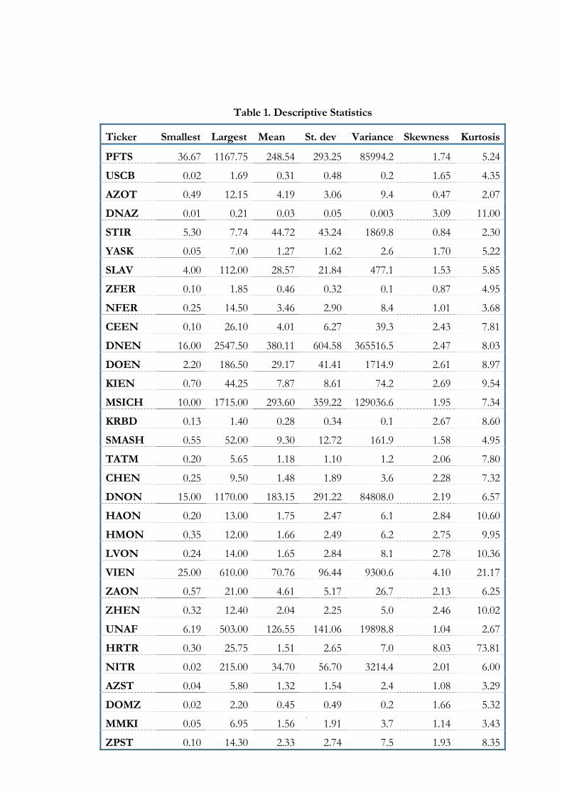
Table 1 presents the summary statistics for the prices in the sample.
Prices are highly volatile, with variance to mean ration from 0.1 for DNAZ to
961.6 for DNEN. Also, skewness and kurtosis are high over the sample,
suggesting non-normal distribution of prices.
10
11
Table 1. Descriptive Statistics
Ticker Smallest Largest Mean St. dev Variance Skewness Kurtosis
PFTS 36.67 1167.75 248.54 293.25 85994.2 1.74 5.24
USCB 0.02 1.69 0.31 0.48 0.2 1.65 4.35
AZOT 0.49 12.15 4.19 3.06 9.4 0.47 2.07
DNAZ 0.01 0.21 0.03 0.05 0.003 3.09 11.00
STIR 5.30 7.74 44.72 43.24 1869.8 0.84 2.30
YASK 0.05 7.00 1.27 1.62 2.6 1.70 5.22
SLAV 4.00 112.00 28.57 21.84 477.1 1.53 5.85
ZFER 0.10 1.85 0.46 0.32 0.1 0.87 4.95
NFER 0.25 14.50 3.46 2.90 8.4 1.01 3.68
CEEN 0.10 26.10 4.01 6.27 39.3 2.43 7.81
DNEN 16.00 2547.50 380.11 604.58 365516.5 2.47 8.03
DOEN 2.20 186.50 29.17 41.41 1714.9 2.61 8.97
KIEN 0.70 44.25 7.87 8.61 74.2 2.69 9.54
MSICH 10.00 1715.00 293.60 359.22 129036.6 1.95 7.34
KRBD 0.13 1.40 0.28 0.34 0.1 2.67 8.60
SMASH 0.55 52.00 9.30 12.72 161.9 1.58 4.95
TATM 0.20 5.65 1.18 1.10 1.2 2.06 7.80
CHEN 0.25 9.50 1.48 1.89 3.6 2.28 7.32
DNON 15.00 1170.00 183.15 291.22 84808.0 2.19 6.57
HAON 0.20 13.00 1.75 2.47 6.1 2.84 10.60
HMON 0.35 12.00 1.66 2.49 6.2 2.75 9.95
LVON 0.24 14.00 1.65 2.84 8.1 2.78 10.36
VIEN 25.00 610.00 70.76 96.44 9300.6 4.10 21.17
ZAON 0.57 21.00 4.61 5.17 26.7 2.13 6.25
ZHEN 0.32 12.40 2.04 2.25 5.0 2.46 10.02
UNAF 6.19 503.00 126.55 141.06 19898.8 1.04 2.67
HRTR 0.30 25.75 1.51 2.65 7.0 8.03 73.81
NITR 0.02 215.00 34.70 56.70 3214.4 2.01 6.00
AZST 0.04 5.80 1.32 1.54 2.4 1.08 3.29
DOMZ 0.02 2.20 0.45 0.49 0.2 1.66 5.32
MMKI 0.05 6.95 1.56 1.91 3.7 1.14 3.43
ZPST 0.10 14.30 2.33 2.74 7.5 1.93 8.35

C h a p t e r 4
MODEL AND METHODOLOGY
Model and Methodology
In my study I adopt the methodology introduced by Balvers, Wu and
Gilliland (2000), Chaudhuri and Wu (2004) and Gropp (2004). Below I
provide some justification for the chosen methodology.
Stochastic process for the price if an asset that shows mean-reversion
is constructed as follows:
1 1( )i i i i fi it t t t tP P a P P 1
iλ ε+ +− = + − + +
it
, (1)
where is the log of the price of stock i, so that (itP 1
itP P+ − ) equals to a
continuously compounded return of investor at time t+1, 1fi
tP+ is the log of
the fundamental value of the stock price index at time t+1, which is
unobserved, 1itε + is the stationary error term. Parameter iλ (0< iλ <1) gives
information about the mean reversion. If iλ is zero, there is no mean
reversion. If iλ is minus one, the full reversion happens in the subsequent
time period.
So, obtaining iλ <0 means conforming the mean-reversion hypothesis.
Detection of the mean-reverting behaviour of the price is complicated by the
need to identify fundamental path that the price is reverting to after shocks.
Researchers have used different proxies for fundamental values.
Cutler et al. (1991) used logarithm of dividend-to-price ratio as a proxy of
12
fundamental value to estimate equation (1). Also, Chiang et al. (1995) use
earnings and dividends per share as a proxy for fundamental value claiming
that a firm’s fundamental value may possibly be expressed as a linear function
of earnings and dividends. One should be very cautious when specifying
fundamental value. Wrong specification of the fundamental path significantly
distorts the results (see Balvers, Wu and Gillliland, 2000).
However, this estimation problem may be resolved by using a
reference index that the stock price is being compared to. A basic assumption
here is that the difference between fundamental values of the stocks and
fundamental value of the reference index is stationary, which can be
expressed as follows:
fi fr it tP P z i
tν= + + , (2)
where itν is the stationary process with zero mean that may be serially
correlated, is a constant, iz frtP stands for the log of the fundamental value of
the reference index.
This assumption has been used by Balvers, Wu and Gillliland (2000)
and Chaudhuri and Wu (2004) for the cross-country indices and by Gropp
(2004) for stock portfolios without particular justification. However, in order
to prove that the results of estimating such a model are consistent with the
theory, some reasoning is required.
In this study, the PFTS index is used as a reference index for the
model. It seems a natural candidate for this role since it possesses the
following qualities that justify such choice:
• PFTS index is a weighted average of the stocks in the sample, and
hence, it “borrows” from variations in each stock’s price;
• A number of same economic variables influence both PFTS index
and individual stocks making them move together to some extent;
13

• Both returns on the PFTS index and on individual stocks are limited
in the long run by economic growth (Damodaran (1994)). This means
that growth in any of the stocks’ price cannot exceed the growth of
the PFTS index infinitely implying stationary difference in their
fundamental values in the long run.
Referring to the valuation theory, the period during which a stock
price outperforms the market is rarely more than five years given that a
company is young (or the IPO has been done recently). Since both a stock
price and market index have same limit – the difference in their prices should
be stationary in the long run. Hence, relying on these facts, the assumption (2)
may be justified.
Using this model specification is also convenient since one should not
account separately for structural breaks in the market (the requirement for
testing for structural breaks was stated by Chaudhuri and Wu (2003),
Valadakhani and Chancharat (2007)). When market is subject to structural
break, it has same impact on stocks and reference index, thus not changing
the fundamental relationship between them.
Further, if one assumes that the speed of mean reversion is same for the
stock and the reference index, then combining equations (1) for the stock i
and the reference index and (2), the following relationship follows:
it
rt
it
irt
it PPRR 111 )( +++ +−+=− ωλα , (3)
where 1itR + = ( 1
i it tP P+ − ), i i ra a ziα λ= − + , and
i i rt t t
itω ε ε λν= − + . Equation 3 is in the form of a standard Dickey-Fuller
(1979) test. If the error term, 1itω + is serially uncorrelated, OLS method can
be used to estimate this equation and t-statistics can be used to test whether
λ is greater than zero. If, however, the error term is serially correlated, one
14

should add to the independent variables lagged values of ( 1it t 1
rR R+ − + ) to
account for serial correlation.
The assumption of similar speeds of mean reversion may seem
unrealistic. Moreover, since this study uses same reference index for all stocks,
this assumption implies same mean reversion for all the stocks in the market.
However, firstly, since all the stocks under consideration are taken from a
single market, they are subject to the same impact of the market forces.
Putting individual companies’ differences aside, the speeds of mean reversions
for different stocks may be quite similar. Still, the assumption of equal speeds
of mean reversion is quite simplifying and may be not the adequate
representation of the reality. Nevertheless, applying this assumption is
inevitable if one wants to receive the characteristics of the stock market
overall and to compare his/her findings with other findings in the field.
Positive value of λ means that accumulated difference in returns
between a stock price and market index signals the investors to reallocate
their money to the stocks that have been underperforming the market.
However, the unit root tests have low power against the random walk
hypothesis when applied to individual stock prices (see Campbell and Perron
(1991), Cochrane (1991). As shown in Balvers, Wu and Gillliland (2000),
panel variant of the test increases the testing power very significantly, while
univariate approach is weak even for substantially long sample. In addition,
the sample size used in this study is rather small for such estimation. Hence,
the non-rejection of the null hypothesis of λ =0 may not be due to non-
existence of the mean reversion in the Ukrainian stock prices but due to small
sample size and low testing power.
The estimating procedure is as follows:
First, univariate tests for individual stocks were performed. The
estimating method is OLS. Lag length was set according to Said and Dickey
(1984): k=T1/3or five in this case. Critical values are taken from Fuller (1976).
It is likely that this test is not able to reject null of no mean-reversion due to
reasons mentioned above.
15

As the second step, estimates of mean reversion for individual stocks
are obtained through SUR estimation. SUR model is used as superior to OLS
since it accounts for variables common to all stocks’ equations and not
included into the model. Although SUR provides stronger coefficients and
smaller standard errors, the estimates are subject to a bias in this case (Levin
and Lin, 1993), thus making the results not fully reliable. But since this
estimation is provided mainly to give some comparative results and given the
tediousness of the bias-correcting procedure, I left the results uncorrected.
This estimation is also used to show approximately how similar are
the speeds of mean reversion for the stocks in our sample. This might show
how good does the assumption of similar mean reversion fit our data.
Afterwards, the estimation of coefficient for overall market mean
reversion follows.
As the main procedure, around which the discussion in this thesis is
built, equation (3) was estimated using SUR under the assumption of equal
speeds of mean reversion for all stocks in the market. Hence, I ran the model
with restriction of equal values of λ for all equations.
The following statistics were used for testing the significance ofλ :
; , λλˆTz = )ˆ(./ˆ λλλ est =
where T is the sample size, $. ( )s e λ is the standard error of λ .
However, under the null hypothesis of λ=0, and presence of unit root in the
data, the estimator of λ is biased and statistics do not have normal limiting
distribution. Presence of a unit root causes the estimator to converge at a
faster rate with growth of number of periods used than with an increase in
cross-sectional units (“super consistency” property). Additionally, if
individual-specific fixed effects or correlations are present, test statistics
converge not to a normal distribution, but to the non-central normal
distribution, which significantly influences the size of the test (Levin and Lin,
1992).
To account for such problems in this estimation, I used Monte Carlo
simulations to construct reliable confidence intervals for the point estimate of
16

λ. In doing so, I draw disturbances form a multivariate normal distribution
with T=951, the number of observations, and N=36, the number of stocks,
and use them to simulate the model, fixing the historical values of the right-
hand side variables in the equations as well as coefficients. Then I ran the
same regression as discussed above to get the simulated value of λ and the test
statistics, and λt . This process was repeated 5,000 times to get simulated
distribution of the coefficients and test statistics. Then the p-values for the
statistics, and λt were calculated as the percentage of statistics from
historic distribution that has larger (negative in this case) values.
λz
λz
Next I addressed the bias in issue. To do this, I constructed the
median-unbiased estimate of λ as discussed in Andrews and Chen (1994). I
conducted several Monte-Carlo simulations similar to the one described
above, but exogenously fixing the values of λ in the model (I did simulations
for λ in the range [-0.01;-0.25] with a step equal to 0.005). I received
distributions of estimates under each particular value of λ from this range.
Then I found values of λ which equated median, 5 and 95 percent of
simulated to the historical . This gives us the median unbiased estimate
of λ as well as its 90 percent confidence interval.
λ̂
s'̂λ λ̂
Finally, I estimated the mean reversion coefficient for the market
using a simple OLS. This type of estimation is a test for robustness of the
results.
1 Dataset gives 97 price observations and 96 returns, however our model includes one lagged value of
returns in the right-hand side, as will be discussed later. This implies T=95 for Monte Carlo.
17

C h a p t e r 5
EMPIRICAL RESULTS
First, equation (3) was estimated univariately, stock by stock, using a
simple OLS. The lag length was chosen according to Said and Dickey (1984)
as 3/1T or five in this case. The test rejected the null of no mean reversion for
2 stocks out of sample of 31. This result is not surprising given a small sample
size and a small size of the test2. The results are presented in Table 2.
As the second step, individual mean reversion coefficients were
estimated using SUR model. In general, this estimation procedure is more
efficient, and that is why the results were expected to be stronger than from
univariate OLS test. The lag length was chosen according to the BIC criterion.
The test rejected random walk in favor of the mean reversion for 28 stocks in
the sample. These results look significantly stronger compared to the first
estimation. However, the coefficients for this regression are biased (Levin and
Lin, 1993) due to a small sample size. As well, confidence intervals are
incorrect. This makes the results of SUR estimation not fully reliable.
However, since these tests were done mostly for comparison of the results as
well as for some insights about price behavior in Ukrainian stock market, they
were not corrected for the bias leaving this procedure for the receiving of a
market estimate of the mean reversion. The results of the test are combined
in Table 3.
Despite the fact that coefficients are biased, since the p-values for
2 The size of the test means the probability of not committing type 1 error (not rejecting the null when
null hypothesis is incorrect)
18
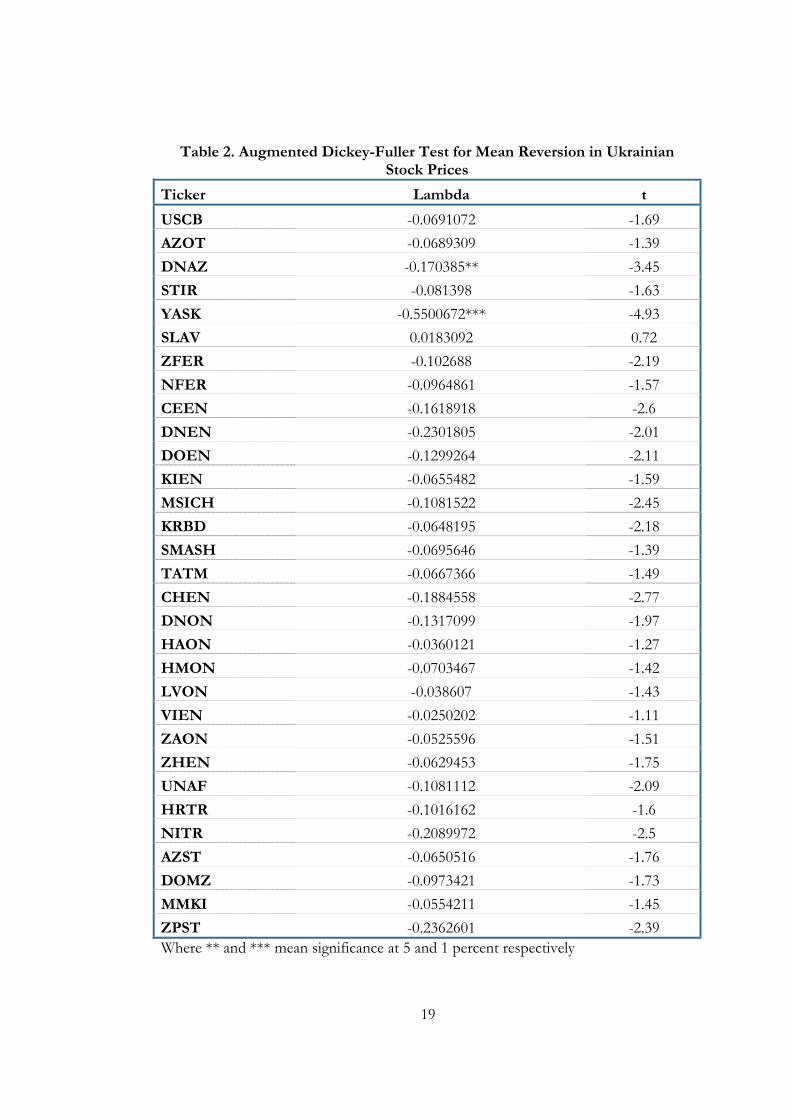
Table 2. Augmented Dickey-Fuller Test for Mean Reversion in Ukrainian Stock Prices
Ticker Lambda t
USCB -0.0691072 -1.69 AZOT -0.0689309 -1.39 DNAZ -0.170385** -3.45 STIR -0.081398 -1.63 YASK -0.5500672*** -4.93 SLAV 0.0183092 0.72 ZFER -0.102688 -2.19 NFER -0.0964861 -1.57 CEEN -0.1618918 -2.6 DNEN -0.2301805 -2.01 DOEN -0.1299264 -2.11 KIEN -0.0655482 -1.59 MSICH -0.1081522 -2.45 KRBD -0.0648195 -2.18 SMASH -0.0695646 -1.39 TATM -0.0667366 -1.49 CHEN -0.1884558 -2.77 DNON -0.1317099 -1.97 HAON -0.0360121 -1.27 HMON -0.0703467 -1.42 LVON -0.038607 -1.43 VIEN -0.0250202 -1.11 ZAON -0.0525596 -1.51 ZHEN -0.0629453 -1.75 UNAF -0.1081112 -2.09 HRTR -0.1016162 -1.6 NITR -0.2089972 -2.5 AZST -0.0650516 -1.76 DOMZ -0.0973421 -1.73 MMKI -0.0554211 -1.45 ZPST -0.2362601 -2.39 Where ** and *** mean significance at 5 and 1 percent respectively
19

most of the coefficients are rather low, it is quite probable that those
coefficients will remain significant, would the correction for the bias be
implemented. What is important is that difference in coefficients across the
stocks is large, ranging from 0.05 for MMKI to 0.35 for NITR, which
suggests that assumption about common speed of mean reversion for all
stocks may be inappropriate. However, the correction for bias may have
somewhat smoothed the variation.
Taking into account that univariate tests did provide some evidence in
favor of the mean reversion for a number of stocks in the sample, even in
spite of the weakness of the procedure, it is natural to expect that more
powerful tests will confirm these findings and will present stronger evidence.
As the second part of estimation process, I searched for the estimate
of the market coefficient of mean reversion. The basic testing procedure
involves estimation of SUR model under the assumption of equal speed of
the mean reversion for all analyzed stocks. Under the null hypothesis of
λ =0, is biased and statistics do not have normal limiting distributions.
Therefore, the bias was accounted for and appropriate critical values were
found using Monte Carlo simulation.
λ̂
The point estimate of λ was found to be -0.093. Following the
procedure discussed in previous section, I calculated reliable p-values for two
statistics, and . As is discussed in Balvers, Wu and Gilliland (2000),
statistics has a superior test size over (lower probability of type 1 error).
Anyway, both statistics imply that is significant at 5% and 1% respectively.
As the structure of the two statistics show, while accounts for the standard
error of the estimate, does not. This is the main reason why implies
higher level of significance in this case: the standard error of is equal to
0.0077 which is very low. Other authors found evidence of slower mean
reversion: Chaudhury and Wu (2004) found point estimate of λ equal -0.274,
for annual return horizon while Gropp (2004) found λ equal from -0.114 to -
0.178 depending on the exchange studied. The possible reasons are discussed
λz λt λz
λt
λ̂
λt
λz λt
λ̂
20

Table 2. Unrestricted SUR estimation of individual mean reversion coefficients
Ticker Lambda Std.Err p-value
USCB -0.0738 0.0317 0.0200 AZOT -0.0833 0.0392 0.0330 DNAZ -0.0839 0.0280 0.0030 STIR -0.1029 0.0363 0.0050 YASK -0.3219 0.0556 0.0000 SLAV -0.0029 0.0179 0.8700 ZFER -0.1240 0.0315 0.0000 NFER -0.1744 0.0416 0.0000 CEEN -0.1678 0.0500 0.0010 DNEN -0.3425 0.0737 0.0000 DOEN -0.1475 0.0444 0.0010 KIEN -0.0843 0.0360 0.0190 MSICH -0.0796 0.0337 0.0180 KRBD -0.0573 0.0248 0.0210 SMASH -0.1322 0.0336 0.0000 TATM -0.0761 0.0331 0.0210 CHEN -0.1555 0.0491 0.0020 DNON -0.1897 0.0468 0.0000 HAON -0.0636 0.0205 0.0020 HMON -0.1362 0.0385 0.0000 LVON -0.0469 0.0198 0.0180 VIEN -0.0384 0.0179 0.0320 ZAON -0.0547 0.0242 0.0240 ZHEN -0.1100 0.0274 0.0000 UNAF -0.1149 0.0411 0.0050 HRTR -0.1059 0.0392 0.0070 NITR -0.3508 0.0550 0.0000 AZST -0.0906 0.0268 0.0010 DOMZ 0.0740 0.0365 0.0430 MMKI -0.0505 0.0292 0.0840 ZPST 0.2847 0.0604 0.0000
21

below, after discussing the median-unbiased estimate of λ.
As the next step, the median-unbiased estimate of λ was calculated
through the procedure discussed in section 3. The reason to use this estimate
is that it has better properties compared to the point estimate (Phillips and Sul
(2002) showed that median unbiased estimate has overall MSE performance 5
times better than the OLS estimate and twice better then the SUR estimate
for small samples with high degree of cross-sectional dependence) 3.
Median-unbiased λ is found to be approximately equal to -0.1077,
which is significantly higher than the point estimate. Other authors, however,
usually find the median-unbiased estimate to be lower than the point estimate
(see Gropp (2004), similar to Balvers, Wu and Gilliland (2000) and Chauhudri
and Wu (2004)). The cause of this may be due to different sample size in the
other studies. While other authors used longer time series and less cross-
sectional observations, in my study the time span is significantly shorter while
cross-sectional richness is higher than in other studies. As it was mentioned
earlier, estimator of λ converges at a faster rate with the growth of the number
of periods than with an increase in cross-sectional units. Hence, this may be
the explanation for such a difference.
The 90 percent confidence interval for the median-unbiased estimate
was found to be [-0.015;-0.205], which is rather wide, compared to other
studies. The median unbiased coefficient implies the half-life of mean
reversion equal to 6 months4. This number is significantly lower compared to
those found previously by other studies, meaning much higher speed of mean
reversion. There might be several explanations for this:
Firstly, as was mentioned in section 1, other studies concentrate
mostly on cross-country analysis, performing tests on countries’ indices.
Although, one should also expect the difference between fundamental values
of index i and the reference index (for example, the World index, as in
3 MSE (mean squared error) gives a measure of an amount by which an estimator differs from the true
value of the parameter. ))ˆ(()ˆ( 2θϑθ −= EMSE4 Half life is calculated as: )ˆ1(/)5.0( λ−LnLn
22

Balvers, Wu and Gilliland (2000)) to be stationary in the long run, it will take
much more time to reach this long run, compared to the case of individual
company stock and PFTS index. Hence, if the time needed for returns in
country’s index to converge to those of the world index is longer, it is natural
that the speed of mean reversion should be smaller.
Secondly, faster mean reversion may be due to appearance of new
rivals in the market which deteriorates financial performance of the
companies as well as their growth prospects. So, prices for stocks for these
companies may show sharp jumps and falls, generating high speed of mean
reversion.
Thirdly, since Ukraine is an emerging capital market, it naturally
experiences overall high price volatility. This may have created the price
pattern that is perceived as high speed mean-reverting returns behavior.
Hence, it may be true that high coefficient received in this study has little to
do with theoretical explanation, but just with natural volatility in prices.
To compare the SUR results with some other models, I have also
conducted a panel OLS estimation of equation (3) to receive market mean
reversion estimate. I chose the lag length similar to the one used for univariate
OLS estimation (L=5). Although the OLS approach is not efficient in this
case, as well as it provides biased estimate of λ, it also suggests that the null of
no mean reversion may be rejected. Still, it significantly underestimates the
magnitude of the coefficient implying weaker mean reversion.
Results of the last two estimation procedures are combined in the
table 4.
23
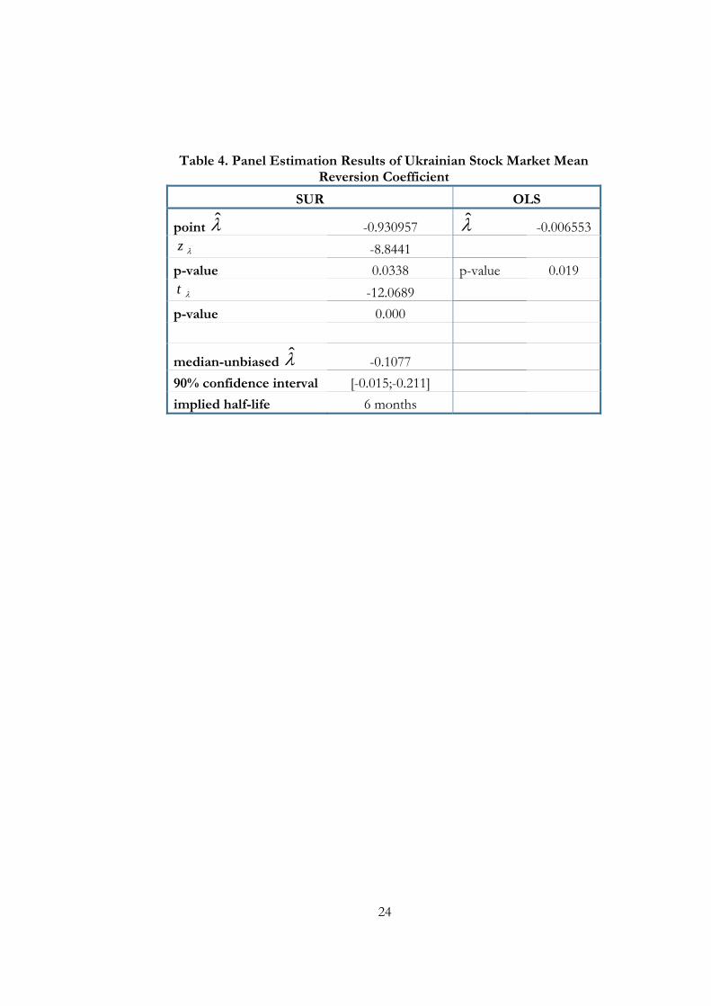
Table 4. Panel Estimation Results of Ukrainian Stock Market Mean Reversion Coefficient
SUR OLS
point λ̂ -0.930957 λ̂ -0.006553λz -8.8441
p-value 0.0338 p-value 0.019 λt -12.0689
p-value 0.000
median-unbiased λ̂ -0.1077 90% confidence interval [-0.015;-0.211] implied half-life 6 months
24

C h a p t e r 6
CONCLUSIONS
This thesis was aimed at checking whether Ukrainian stock market is
experiencing mean reversion in stock prices. To achieve this goal, several
estimating methods were used. At the first step, ADF test was applied to
equation (3) stock by stock. This test has low power to reject null of mean
reversion and was able only to confirm mean reversion hypothesis for two
stocks out of 31.
At the next step, unrestricted SUR model was used. It is more
powerful and suggested stronger evidence in favor of mean reversion across
stocks in the sample. The estimators implied by this procedure are subject to
small sample bias and might not be reliable. Still, most of the p-values are
quite low, which might suggest that ’s should remain significant if the bias
correcting procedure was implemented.
λ̂
To estimate the overall market mean reversion coefficient, I used
restricted SUR model, whether the restriction in that all ’s are constrained to
be equal. The estimates from this model are also subject to small sample bias.
This bias was accounted for through constructing reliable confidence intervals
with Monte Carlo simulations and median-unbiased estimate of λ which has
superior MSE performance over the point estimate. Median unbiased was
found to be equal to -0.1077, thus implying the half-life of mean reversion of
6 months. This implies much faster mean reversion than found in other
studies. There might be several reasons for such result. First is that I studied
mean reversion in the market of one country, while comparable studies were
mostly concentrated on cross-country investigations. Second is that Ukrainian
market is young and companies’ performance might not be smooth over time,
thus creating jumps and falls in stock price that is perceived as higher speed of
λ̂
λ̂
25

mean reversion. Third is that Ukrainian stock market is subject to natural
price volatility as a young one. This price volatility that has nothing to do with
financial theory that tries explaining mean reversion, however, is able to form
high-speed mean reverting stock price behavior.
OLS regression also suggests that mean reversion is present in
Ukrainian market, but it estimates that speed of mean reversion is lower than
implied by SUR technique.
To add things up, this study found strong evidence in favor of mean
reversion in Ukrainian stock market. There may be a number of reasons for
such results. However, it is hard to distinguish which one is the main cause
for mean reversion. There is a big chance that big proportion of what is
perceived as mean reversion is due to high natural stock price volatility.
26

C h a p t e r 7
CONCLUDING REMARKS
This section discusses the limitations of the approach used in this
thesis and the future steps to be implemented in the field of study.
There are several drawbacks of this study:
First, it is assumed that stocks in the market as well as the reference
index have same speed of mean reversion to their fundamental values. As we
saw from the unrestricted SUR estimation, discussed in Chapter 4, the
estimated coefficients for mean reversion are rather different across the
stocks. This may have caused distortion of the results.
Second, the dataset contained very little time observations, which may
cause general non-representativeness of the results received. There are too
little stocks that were actually traded before 2000, so the data lacks price
variability. With time pass, more long and reliable data series will be available
so that more reliable estimates may be received.
Third, since the market possesses high natural price volatility, it is
impossible to distinguish between mean reversion and random price
movements that simulate mean reverting processes. To make the results more
clear, it would be very helpful to filter out the portion of random movements
of stock prices. However, until now there is no particular method developed
for this.
Also, it is important to find out whether the results of the studies that
used different return horizons may be directly compared. Gropp (2004)
reports results for different return horizons and the speed of mean reversion
he receives is proportional to the return horizon (he found λ’s equal 0.136,
0.275 and 0.387 for NYSE index and 0.114, 0.230, 0.346 for index that he
27

constructed himself, for 1, 2 and 3 years return horizon respectively).
However, there are no statistical evidence that speed of mean reversion
increases proportionately as the return horizon increases. Thus, while I
received very high speed of mean reversion, compared to other studies, this
may be due to non-comparability of the return horizons used.
28

BIBLIOGRAPHY
Andrews, Donald, and Hong-Yuan,Chen, Approximately Median-Unbiased Estimation of Autoregressive
Models, Journal of Business and Economic Statistics, 1994,
12(2), 187-204.
Balvers, Ronald, Wu, Yangru, Gilliland, Eric, Mean Reversion
Across National Stock Markets and Parametric Contrarian Investment
Strategies, The Journal of Finance, Vol. 2, 2000, 745-772.
Campbell, John Y., and Perron, Pierre, Pitfalls and Opportunities: What macroeconomist should know
about unit roots, NBER Macroeconomics Annual, MIT
Press, Boston, 1991.
Cecchetti, Stephen, Pok-Sang, Lam and Nelson, Mark, Mean reversion in
equilibrium asset prices, American Economic Review, 1990, 80, 398–
418.
Chaudhuti, Kausik and Wu, Yangru, Random Walk Versus Breaking Trend in Stock Prices: Evidence
From Emerging Markets, Journal of Banking and Finance, 2003,
Elsevier, vol 27(4)
Chaudhuti, Kausik and Wu, Yangru, Mean Reversion in Stock Prices:
Evidence From Emerging Markets, Managerial Finance, 2004,
vol.30, 22-37.
Chiang, R., Liu, P., Okunev, J., Modelling mean reversion of asset prices
towards their fundamental value,
Journal of Banking and Finance , 1995, 19, 1327– 1340.
Cochrane, John H., A Critique of the
Application of Unit Root Tests, Journal of Economic Dynamics and Control,1991, 15, 275-284.
Cutler, David M., Poterba, JamesM.,
and Summers, Lawrence H., Speculative dynamics, Review of Economic Studies, 1991, 58,
529-546.
Damodaran, A., Damodaran on Valuation, 1994, Wiley, New
York, NY.
DeBondt, Werner and Thaler, Richard, Further Evidence of
Overreaction and Stock Market Seasonality, Journal of Finance,
1987, 42, 557-581.
DeBondt, Werner, and Thaler, Richard, Does the Stock Market
Overreact?, Journal of Finance,1985 40, 793–805.
DeJong, David N. et al., The Power
Problems of Unit Root Tests in Time Series with Autoregressive Errors,
Journal of Econometrics, 1992 53, 323-343.
Dickey, David A., and Fuller,
Wayne A., Distribution of the Estimators for Autoregressive Time Series wit a Unit Root, Journal of
the American Statistical Association,1979, 74, 427-481.
Engel, Charles and Morris,
29

Charles S., Challenges to Stock Market Efficiency: Evidence from Mean Reversion Studies, Economic
Review, 1991
Fama, Eugene and French, Kenneth, Permanent and
Temporary Components of Stock Prices, Journal of Political
Economy, 1988, 96, 246-273.
Fuller, Wayne A.., Introduction to Statistical Time Series, 1976, John
Wiley and Sons, New York.
Kim, Myung Jig, Nelson, Charles R., and Startz, Richard, Mean
Reversion in Stock Prices? A Reappraisal of the Empirical
Evidence, Review of Economic Studies, 1991, 58, 151-528.
Levin, Andrew and Lin, Chien-Fu,
Unit Rot Tests in Panel Data: Asymptotic and Finite Sample
Properties, 1993, Mimeo, University of California, San
Diego.
Lo, Andrew and MacKinlay, Craig A., Stosk Market Prices Do Not Follow Random Walks: Evidence From a Single Specification Test, Review of Financial Studies,
1988, 1, 41-66.
Malkiel, Burton, A Random Walk Down Wall Street, 2000, W.W.
Norton & Company.
McQueen, Grant, Long-Horizon Mean-Reverting Stock Prices Revisited, The
Journal of Financial and Quantitative Analysis, 1992,
Vol. 27, No. 1, pp. 1- 18
Perron, Pierre, Testing of a Random Walk: A Simulation Experiment of Power When the Sample Interval is
Varied, Advances in Econometrics and Modelling,
1989, Kluwer, Boston.
Perron, Pierre, Test Consistency with Varying Sampling Frequency,
Econometric Theory, 1991, 7, 341-368.
Phillips PCB, Sul D, Dynamic panel estimation and homogeneity testing
under cross section dependence. Cowles Foundation Discussion
Paper, 2002, n. 1362
Poterba, James and Summers, Lawrence, Mean Reversion in
Stock Prices: Evidence and Implications, Journal of Business and Economic Statistics, 1988,
22, 27-59.
Richardson, Matthew, Temporary Components of Stock Prices: a
Sceptic’s View, Journal of Business and Economic
Statistics, 1993, 11, 199-207.
Said, S.E., and Dickey, David A., Testing for Unit Roots in
Autoregressive Moving Average Models of Unknown Order,
Biometrica, 1984, 71, 599-608.
Samuelson, Paul, Proof That Properly Anticipated Prices
Fluctuate Randomly,Industrial Management Review, Vol. 6,
No. 2, pp. 41-49.
30

Valadakhani, A. and Chancharat, S, Structural Breaks in Testing for the
Random Walk Hypothesis in International Stock Prices, Journal
of The Korean Economy, 2007, 8(1), 21-38.
31

32

4
Recommended