Introduction Hausman (96) Consumer Welfare using the DC Model
Measurement of Consumer WelfareNBER Methods Lectures
Aviv Nevo
Northwestern University and NBER
July 2012

Introduction Hausman (96) Consumer Welfare using the DC Model
Introduction
� A common use of empirical demand models is to computeconsumer welfare
� We will focus on welfare gains from the introduction of newgoods
� The methods can be used more broadly:� other events: e.g., mergers, regulation� CPI
� In this lecture we will cover� Hausman (96): valuation of new goods using demand inproduct space
� consumer welfare in DC models

Introduction Hausman (96) Consumer Welfare using the DC Model
Hausman, �Valuation of New Goods Under Perfect andImperfect Competition�(NBER Volume, 1996)
� Suggests a method to compute the value of new goods underperfect and imperfect competition
� Looks at the value of a new brand of cereal �AppleCinnamon Cheerios
� Basic idea:� Estimate demand� Compute �virtual price��the price that sets demand to zero� Use the virtual price to compute a welfare measure (essentiallyintegrate under the demand curve)
� Under imperfect competition need to compute the e¤ect of thenew good on prices of other products. This is done bysimulating the new equilibrium

Introduction Hausman (96) Consumer Welfare using the DC Model
Data
Monthly (weekly) scanner data for RTE cereal in 7 cities over 137weeks
Note: the frequency of the data. Also no advertising data.

Introduction Hausman (96) Consumer Welfare using the DC Model
Multi-level Demand Model� Lowest level (demand for brand wn segment): AIDS
sjt = αj + βj ln(ygt/πgt ) +Jg
∑k=1
γjk ln(pkt ) + εjt
where,� sjt dollar sales share of product j out of total segmentexpenditure
� ygt overall per capita segment expenditure� πgt segment level price index� pkt price of product k in market t.
πgt (segment price index) is either Stone logarithmic price index
πgt =Jg
∑k=1
skt ln(pkt )
or
πgt = α0 +Jg
∑k=1
αkpk +12
Jg
∑j=1
Jg
∑k=1
γkj ln(pk ) ln(pj ).

Introduction Hausman (96) Consumer Welfare using the DC Model
Multi-level Demand Model
� Middle level (demand for segments)
ln(qgt ) = αg + βg ln(YRt ) +G
∑k=1
δk ln(πkt ) + εgt
where
� qgt quantity sold of products in the segment g in market t� YRt total category (e.g., cereal) expenditure� πkt segment price indices

Introduction Hausman (96) Consumer Welfare using the DC Model
Multi-level Demand Model
� Top level (demand for cereal)
ln(Qt ) = β0 + β1 ln(It ) + β2 lnπt + Ztδ+ εt
where
� Qt overall consumption of the category in market t� It real income� πt price index for the category� Zt demand shifters

Introduction Hausman (96) Consumer Welfare using the DC Model
Estimation
� Done from the bottom level up;
� IV: for bottom and middle level prices in other cities.
Introduction Hausman (96) Consumer Welfare using the DC Model
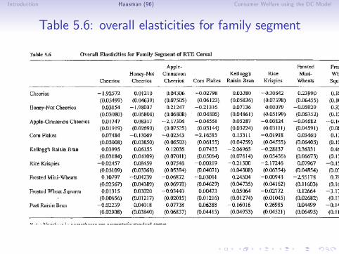
Table 5.6: overall elasticities for family segment

Introduction Hausman (96) Consumer Welfare using the DC Model
Welfare
� Value of AC-Cheerios� Under perfect competition approx. $78.1 million per year forthe US
� Imperfect competition: needs to simulate the world withoutAC Cheerios
� assumes Nash Bertrand� ignores e¤ects on competition� �nds approx $66.8 million per year;
� Extrapolates to an overall bias in the CPI 20%-25% bias.

Introduction Hausman (96) Consumer Welfare using the DC Model
Comments
� Most economists �nd these numbers too high� are they really?
� Questions about the analysis� IVs (advertsing)� computation of Nash equilibrium (has small e¤ect)

Introduction Hausman (96) Consumer Welfare using the DC Model
Consumer Welfare Using the Discrete Choice Model� Assume the indirect utility is given by
uijt = xjtβi + αipjt + ξ jt + εijt
εijt i.i.d. extreme value� The inclusive value (or social surplus) from a subsetA � f1, 2, ..., Jg of alternatives:
ωiAt = ln
∑j2Aexp
�xjt βi � αi pjt + ξ jt
!� The expected utility from A prior to observing (εi0t , ...εiJt ),knowing choice will maximize utility after observing shocks.
� Note� If no hetero (βi = β, αi = α) IV captures average utility in thepopulation;
� wn hetero need to integrate over it� if utility linear in price convert to dollars by dividing by αi� with income e¤ects conversion to dollars done by simulation

Introduction Hausman (96) Consumer Welfare using the DC Model
Applications
� Trajtenberg (JPE, 1989) estimates a (nested) Logit modeland uses it to measure the bene�ts from the introduction ofCT scanners
� does not control for endogeneity (pre BLP) so gets positiveprice coe¢ cient
� needs to do "hedonic" correction in order to do welfare
� Petrin (JPE, 2003) uses the BLP data to repeat theTrajtenberg exercise for the introduction of mini-vans
� adds micro moments to BLP estimates� predictions of model with micro moments more plausible� attributes this to "micro data appear to free the model from aheavy dependence on the idiosyncratic logit �taste� error
Introduction Hausman (96) Consumer Welfare using the DC Model
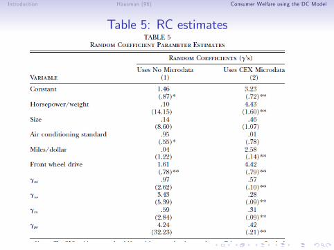
Table 5: RC estimates

Introduction Hausman (96) Consumer Welfare using the DC Model
Table 8: welfare estimates

Introduction Hausman (96) Consumer Welfare using the DC Model
Discussion
� The micro moments clearly improve the estimates and helppin down the non-linear parameters
� What is driving the change in welfare?� One option
� welfare is an order statistic� by adding another option we increase the number of draws� hence (mechanically) increase welfare� as we increase the variance of the RC we put less and lessweight on this e¤ect

Introduction Hausman (96) Consumer Welfare using the DC Model
A di¤erent take
� The analysis has 2 steps1. Simulate the world withoutnwith minivans (depending on thestarting point)
2. Summarize the simulatednobserved prices and quantities into awelfare measure
� Both steps require a model� If we observe pre- and post- introduction data might avoidstep 1
� does not isolate the e¤ect of the introduction
� Logit model fails (miserably) in the �rst step, but can dealwith the second
� just to be clear: heterogeneity is important� NOT advocating for the Logit model� just trying to be clear where it fails

Introduction Hausman (96) Consumer Welfare using the DC Model
Red-bus-Blue-bus problem Debreu (1960)
� Originally, used to show the IIA problem of Logit
� Worst case scenario for Logit� Consumers choose between driving car to work or (red) bus
� working at home not an option� decision of whether to work does not depend on transportation
� Half the consumers choose a car and half choose the red bus� Arti�cially introduce a new option: a blue bus
� consumers color blind� no price or service changes
� In reality half the consumers choose car, rest split between thetwo color buses
� Consumer welfare has not changed
Introduction Hausman (96) Consumer Welfare using the DC Model
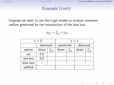
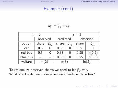
Example (cont)
Suppose we want to use the Logit model to analyze consumerwelfare generated by the introduction of the blue bus
uijt = ξ jt + εijt
t = 0 t = 1observed predicted observed
option share ξ j0 share ξ j1 share ξ j1car 0.5
red bus 0.5blue bus �welfare

Introduction Hausman (96) Consumer Welfare using the DC Model
Example (cont)
uijt = ξ jt + εijt
t = 0 t = 1observed predicted observed
option share ξ j0 share ξ j1 share ξ j1car 0.5 0
red bus 0.5 0blue bus � �welfare ln(2)
normalizing ξcar0 = 0, therefore ξbus0 = 0

Introduction Hausman (96) Consumer Welfare using the DC Model
Example (cont)
uijt = ξ jt + εijt
t = 0 t = 1observed predicted observed
option share ξ j0 share ξ j1 share ξ j1car 0.5 0 0.33 0
red bus 0.5 0 0.33 0blue bus � � 0.33 0welfare ln(2) ln(3)
If nothing changed, one might be tempted to hold ξ jt �xed.This is the usual result: with predicted shares Logit gives gains

Introduction Hausman (96) Consumer Welfare using the DC Model
Example (cont)
uijt = ξ jt + εijt
t = 0 t = 1observed predicted observed
option share ξ j0 share ξ j1 share ξ j1car 0.5 0 0.33 0 0.5
red bus 0.5 0 0.33 0 0.25blue bus � � 0.33 0 0.25welfare ln(2) ln(3)
Suppose we observed actual shares
Introduction Hausman (96) Consumer Welfare using the DC Model
Example (cont)
uijt = ξ jt + εijt
t = 0 t = 1observed predicted observed
option share ξ j0 share ξ j1 share ξ j1car 0.5 0 0.33 0 0.5 0
red bus 0.5 0 0.33 0 0.25 ln(0.5)blue bus � � 0.33 0 0.25 ln(0.5)welfare ln(2) ln(3) ln(2)
To rationalize observed shares we need to let ξ jt varyWhat exactly did we mean when we introduced blue bus?
Introduction Hausman (96) Consumer Welfare using the DC Model
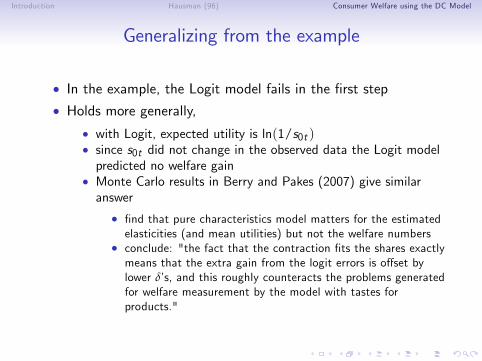
Generalizing from the example
� In the example, the Logit model fails in the �rst step� Holds more generally,
� with Logit, expected utility is ln(1/s0t )� since s0t did not change in the observed data the Logit modelpredicted no welfare gain
� Monte Carlo results in Berry and Pakes (2007) give similaranswer
� �nd that pure characteristics model matters for the estimatedelasticities (and mean utilities) but not the welfare numbers
� conclude: "the fact that the contraction �ts the shares exactlymeans that the extra gain from the logit errors is o¤set bylower δ�s, and this roughly counteracts the problems generatedfor welfare measurement by the model with tastes forproducts."

Introduction Hausman (96) Consumer Welfare using the DC Model
Generalizing from the example
� With more heterogeneity. Logit will get second step wrong� di¤erence with RC
ln�1s0,t
�� ln
�1
s0,t�1
�= ln
�s0,t�1s0,t
�= ln
�Rsi ,0,t�1dPτ(τ)Rsi ,0,tdPτ(τ)
�andZ �
ln�
1si ,0,t
�� ln
�1
si ,0,t�1
��dPτ(τ) =
Zln�si ,0,t�1si ,0,t
�dPτ(τ)
� the di¤erence depends on the change in the heterogeneity inthe probability of choosing the outside option, si ,0,t
� di¤erence can be positive or negative

Introduction Hausman (96) Consumer Welfare using the DC Model
Final comments
� The key in the above example is that ξ jt was allowed tochange to �t the data.
� This works when we see data pre and post (allows us to tellhow we should change ξ jt)
� What if we do not not have data for the counterfactual?� have a model of how ξjt is determined� make an assumption about how ξjt changes� bound the e¤ects
� Nevo (ReStat, 2003) uses the latter approach to computeprice indexes based on estimated demand systems
Recommended