University of Central Florida University of Central Florida
STARS STARS
Electronic Theses and Dissertations
2011
Measurements in Air-water Bubbly Flow Through a Vertical Measurements in Air-water Bubbly Flow Through a Vertical
Narrow High-aspect Ratio Channel Narrow High-aspect Ratio Channel
Benjamin R. Patrick University of Central Florida
Part of the Mechanical Engineering Commons
Find similar works at: https://stars.library.ucf.edu/etd
University of Central Florida Libraries http://library.ucf.edu
This Masters Thesis (Open Access) is brought to you for free and open access by STARS. It has been accepted for
inclusion in Electronic Theses and Dissertations by an authorized administrator of STARS. For more information,
please contact [email protected].
STARS Citation STARS Citation Patrick, Benjamin R., "Measurements in Air-water Bubbly Flow Through a Vertical Narrow High-aspect Ratio Channel" (2011). Electronic Theses and Dissertations. 6659. https://stars.library.ucf.edu/etd/6659

MEASUREMENTS IN AIR-WATER BUBBLY FLOW THROUGH A
VERTICAL NARROW HIGH-ASPECT RATIO CHANNEL
by
BENJAMIN R PATRICK
B.S.M.E. University of Central Florida, 2008
A thesis submitted in partial fulfillment of the requirements
for the degree of Master in Science in Mechanical Engineering
in the department of Mechanical, Materials and Aerospace Engineering
in the College of Engineering and Computer Science
at the University of Central Florida
Orlando, Florida
Summer Term
2011

ii
© 2011 Benjamin R. Patrick
iii
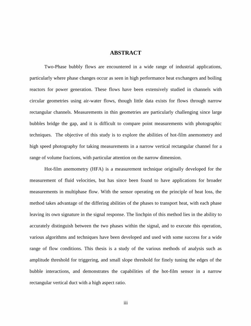
ABSTRACT
Two-Phase bubbly flows are encountered in a wide range of industrial applications,
particularly where phase changes occur as seen in high performance heat exchangers and boiling
reactors for power generation. These flows have been extensively studied in channels with
circular geometries using air-water flows, though little data exists for flows through narrow
rectangular channels. Measurements in thin geometries are particularly challenging since large
bubbles bridge the gap, and it is difficult to compare point measurements with photographic
techniques. The objective of this study is to explore the abilities of hot-film anemometry and
high speed photography for taking measurements in a narrow vertical rectangular channel for a
range of volume fractions, with particular attention on the narrow dimension.
Hot-film anemometry (HFA) is a measurement technique originally developed for the
measurement of fluid velocities, but has since been found to have applications for broader
measurements in multiphase flow. With the sensor operating on the principle of heat loss, the
method takes advantage of the differing abilities of the phases to transport heat, with each phase
leaving its own signature in the signal response. The linchpin of this method lies in the ability to
accurately distinguish between the two phases within the signal, and to execute this operation,
various algorithms and techniques have been developed and used with some success for a wide
range of flow conditions. This thesis is a study of the various methods of analysis such as
amplitude threshold for triggering, and small slope threshold for finely tuning the edges of the
bubble interactions, and demonstrates the capabilities of the hot-film sensor in a narrow
rectangular vertical duct with a high aspect ratio.
iv
A vertical acrylic test section was fabricated for the purposes of this study, inset with a
rectangular channel 38.1mm in width and 3.125mm in depth. Experiments were conducted for
volume fractions ranging from 2% to 35%, which remained within the limits of the bubbly flow
regime, but ranged from small uniform bubbles to larger bubbles coalescing into a transition
regime.
The hot-film signal was analyzed for void fraction, bubble speed, and bubble size. An in-
depth study of the various methods of phase discrimination was performed and the effect of
threshold selection was examined. High-speed video footage was taken in conjunction with the
anemometer data for a detailed comparison between methods. The bubble speed was found to be
in close agreement between the HFA and high-speed video, staying within 10% for volume
fractions above 10%, but still remaining under a 30% difference for even as low as the 2%
volume fraction, where measurements have been found to be historically difficult. The trends
with volume fraction between the HFA and high-speed results were very similar. A correlation
for narrow rectangular channels employing a simple drift flux model was found to compare with
the void fraction data where appropriate. Good agreement was found between the methods using
a hybrid phase discrimination technique for the HFA data for the void fraction and bubble speed
results, with the high-speed video results showing a slight over-estimation in regards to the
bubble size.
v
TABLE OF CONTENTS
LIST OF FIGURES ...................................................................................................................... vii
LIST OF TABLES .......................................................................................................................... x
CHAPTER ONE: INTRODUCTION ............................................................................................. 1
CHAPTER TWO: LITERATURE REVIEW ................................................................................. 5
Air-Water Flow in Vertical Rectangular Channels ..................................................................... 5
Hot-Film Anemometer Signal Response in Multiphase Flow .................................................... 7
Hot-Film Anemometer Signal Analysis.................................................................................... 11
CHAPTER THREE: METHODOLOGY ..................................................................................... 13
Experimental Facility ................................................................................................................ 13
Air-Water Test Loop Overview ............................................................................................ 13
Vertical Test Section ............................................................................................................. 14
Transverse Mechanism ......................................................................................................... 15
Hot-Film Anemometer Data Acquisition System ................................................................. 18
High Speed Camera .............................................................................................................. 19
HFA Signal Analysis ................................................................................................................ 20
Phase Discrimination and Void Fraction .............................................................................. 20
Void Fraction ........................................................................................................................ 21
Bubble Speed ........................................................................................................................ 22
Bubble Size ........................................................................................................................... 23
High Speed Camera Image Analysis ........................................................................................ 23
vi
CHAPTER FOUR: RESULTS AND DISCUSSION ................................................................... 26
Cases Run.................................................................................................................................. 26
Comparison of Phase Discrimination Methods ........................................................................ 29
Void Fraction ............................................................................................................................ 40
Bubble Speed ............................................................................................................................ 44
Bubble Size ............................................................................................................................... 47
CHAPTER FIVE: CONCLUSIONS ............................................................................................ 51
APPENDIX A: LOCATING CHANNEL CENTER .................................................................... 53
APPENDIX B: ERROR PROPOGATION AND UNCERTAINTY ........................................... 56
APPENDIX C: HFA SIGNAL ANALYSIS CODE ..................................................................... 60
Pure Slope Phase Discrimination and Void Fraction Calculation Code ................................... 61
Hybrid (Amplitude Trigger) Phase Discrimination and Void Fraction Calculation Code ....... 62
Bubble Velocity Cross Correlation Code ................................................................................. 64
Chord Length Distribution and Average Diameter Code ......................................................... 67
LIST OF REFERENCES .............................................................................................................. 70

vii
LIST OF FIGURES
Figure 1: Parallel Sensor Hot-Film Probe ....................................................................................... 2
Figure 2: Flow Regime and Transition Regimes for Vertical Narrow Rectangular Channels. (a)
Bubbly, (b) Cap-Bubbly, (c) Slug, (d) Slug-Churn Transition, (e) Churn Turbulent, (f) Annular
[6] .................................................................................................................................................... 5
Figure 3: Flow Regime Map and Transition Lines for a Narrow Rectangular Duct [12],[16] ....... 7
Figure 4: Typical Signal Response to Bubble Passage. A. Front interface, B. Rear interface, C.
Detachment tail collapse, D. Return to liquid phase [18] ............................................................... 8
Figure 5: Probe Interfacial Meniscus Interactions. Left Front Interface, Right Rear Interface [19]
......................................................................................................................................................... 9
Figure 6: Non-Typical Bubble Signal Responses. (a) Vibrating Film, (b) Film Breakage, (c)
Film Vibration then Break, (d) Two Consecutive Bubbles with Film Breaks [19] ...................... 10
Figure 7: Air-Water Test Loop Schematic.................................................................................... 14
Figure 8: Vertical Test Section Diagram ...................................................................................... 15
Figure 9: Transverse Mechanism Schematic ................................................................................ 16
Figure 10: Photograph of the Transverse Mechanism .................................................................. 17
Figure 11: Transverse Mechanism Exploded and Isometric Views ............................................. 18
Figure 12: Image Processing Technique ....................................................................................... 24
Figure 13: Map of Superficial Liquid and Gas Velocities Examined ........................................... 27
Figure 14: Sample Images from Volume Fraction of 2.2% .......................................................... 28
Figure 15: Sample Images from Volume Fraction of 15.2% ........................................................ 28

viii
Figure 16: Sample Images from Volume Fraction of 35.3% ........................................................ 28
Figure 17: Sample of Hot Film Anemometer Signal Response - Amplitude ............................... 29
Figure 18: Sample of Hot Film Anemometer Signal Response – Slope....................................... 30
Figure 19: Amplitude Threshold Selection - Voltage Histogram ................................................. 31
Figure 20: Amplitude Threshold Selection - Void Fraction vs. Threshold .................................. 32
Figure 21: Amplitude Threshold Selection – Derivative of Void Fraction vs. Threshold ........... 32
Figure 22: Amplitude Threshold Selection - Chord Length vs. Threshold .................................. 33
Figure 23: Slope Threshold Selection - Void Fraction vs. Threshold .......................................... 34
Figure 24: Slope Threshold Selection - Derivative of Void Fraction vs. Threshold .................... 35
Figure 25: Slope Threshold Selection - Chord Length vs. Threshold .......................................... 36
Figure 26: Threshold Selection Comparison - Void Fraction ....................................................... 38
Figure 27: Phase Discrimination Method and Threshold Selection Comparison ......................... 39
Figure 28: Channel Averaged Void Fraction Comparison ........................................................... 41
Figure 29: Sample Channel Width Void Fraction Profiles – High Speed Photography ............... 42
Figure 30: Sample Channel Depth Void Fraction Profiles – HFA ............................................... 42
Figure 31: Channel Center Void Fraction Comparison ................................................................ 43
Figure 32: Sample Channel Width Bubble Speed Profiles – High Speed Photography (Bars show
one std. dev.) ................................................................................................................................. 44
Figure 33: Sample Channel Depth Bubble Speed Profiles - HFA ................................................ 45
Figure 34: Bubble Speed Comparison - Volume Fraction ............................................................ 46
Figure 35: Bubble Speed Comparison – Percent Difference between HFA and High Speed
Photography .................................................................................................................................. 46

ix
Figure 36: Sample Channel Width Bubble Size Profiles – High Speed Photography (Bars show
one std. dev.) ................................................................................................................................. 47
Figure 37: Sample Channel Depth Bubble Size Profiles – HFA (Bars show one std. dev.) ........ 48
Figure 38: Bubble Size Comparison - Volume Fraction .............................................................. 49
Figure 39: Bubble Size Comparison – Percent Difference ........................................................... 50
Figure 40: Channel Depth Tests Results ....................................................................................... 55
x
LIST OF TABLES
Table 1: Test Matrix...................................................................................................................... 26
Table 2: Phase Discrimination Method and Threshold Selection Comparison ............................ 36
Table 3: HFA and Camera Uncertainty Analysis ......................................................................... 57
1
CHAPTER ONE: INTRODUCTION
The study of two-phase flows has been largely conducted for medium to large vertical
circular tubes, and has become a well established field, though large interest lies in flows through
channels with alternative geometries. Narrow rectangular channels have presented themselves of
particular interest for its industrial applications as well as for fundamental experimentation in the
development of instrumentation and modeling [1],[2],[3],[4]. Industrial uses include heat
exchangers in small electronics and machines where high-performance cooling is required in
small spaces, as well as in power generation where the narrow rectangular geometries have
applications in evaporator channels [5]. Unlike in larger channels, bubbles in narrow channels
can quickly become large enough to bridge the gap between the walls, leading to entirely
different flow effects and regimes than that seen in larger channels [6]. The flat walls of the
channel lend themselves to the use of optical measurements such as gamma densitometry, laser
Doppler velocimetry, and high speed video [7], [8], but this bridging of the gap effect leads to
difficulty in interpreting the optical data for what occurs along the narrow dimension of the flow.
For this purpose a hot-film anemometer has been paired with high-speed photography to
examine both the wide and narrow dimension of flow, and to compare to each other where
possible.
Hot-wire anemometry is a well established method for measuring flow properties in
single phase systems. They are valued for their simplicity of use as well as minimal
intrusiveness. Hot-film sensors consist of miniscule quartz tube coated by a thin-film of
platinum, as opposed to a single thin wire. Though inherently fragile due to its size, hot-film

2
sensors are considered to be much more robust than their hot-wire counterparts, as the quartz
provides extra rigidity, giving the slightly larger diameter. Typical sensor diameters for hot-wire
probes range from .5 to 5µm, and hot-film sensors range from 25 to 50µm [9]. The probe
acquired for this study is a TSI model 1244-20W parallel hot-film sensor probe, which has two
sensors a known distance apart for the purpose of tracking the speed of flow effects, in this case
bubble interfaces. This probe can be seen pictured below.
Figure 1: Parallel Sensor Hot-Film Probe
There are multiple ways of using these sensors to read the flow characteristics, all relying
on the heat transfer capabilities of the flow of interest. The anemometer acquired for this project
is what is known as a constant temperature anemometer (CTA), though in electrical terms it is
considered to be held at a constant resistance. The resistance of highly conductive metals can be
directly related to their temperature, thus by controlling the resistance of the sensor element, the
temperature is also directly controlled. The IFA 300 uses a Wheatstone bridge electrical
configuration to maintain the sensor at a constant resistance [10]. As convective heat losses to
3
the fluid increases, the amount of power supplied to the sensor must also increase to maintain the
constant temperature/resistance. The power level is varied by an increasing and decreasing
voltage across the sensor, and this voltage history is then in turn converted to a digital signal and
recorded by a high-speed data acquisition system. The principle of usage in multiphase flow
comes from the differences in thermal conductivity between two phases, each phase having
distinct heat transfer properties. The phase with the higher thermal conductivity will cause
higher heat losses and report higher voltages, alternatively the phase with the lower conductivity
will absorb less heat, and report lower voltages. The crux of the analysis is differentiating
between the two phases within the signal, and once this is done the flow properties are easily
derived.
This study compares the various methods of phase discrimination of the HFA signal,
using new techniques to take an in depth look at threshold selection for both amplitude and slope
triggering. After finding satisfaction with a hybrid method of phase discrimination, and a
threshold selection based on physical principles, the results were analyzed for void fraction,
bubble speed, and bubble size. High-speed video was also taken, using MATLAB’s very robust
image processing capabilities to quickly and accurately analyze results. Results from center of
the images could be compared with the HFA, being centered on the channel, with the full image
being compared with a correlation formulated on the drift flux model for the entire channel.
The test section used for this study is oriented vertically with a rectangular channel
38.1mm in width and 3.125mm in depth. Flow straighteners at the entrance of the channel
ensure a uniform flow before the bubbles are injected using a porous sparging stone, similar to
that employed by [11]. The conditions for the experiments were well controlled and span across

4
the limits of the bubbly flow regime. Volume fractions studied range from as low as 2% to as
high as 35%, reaching into cap-bubbly transition regime.
5
CHAPTER TWO: LITERATURE REVIEW
Air-Water Flow in Vertical Rectangular Channels
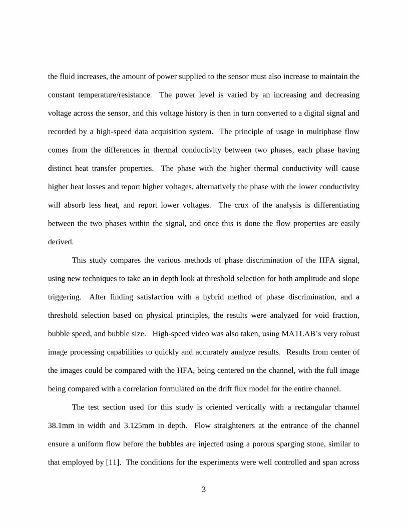
Mishima et al. [12] studied vertical narrow channels with gaps raging from 1mm to 5mm
using neutron radiography and high-speed video. Flow regime maps were generated from the
high-speed video for channel gaps of 1.0mm, 2.4mm, and 5.0mm considering bubbly flow, slug
flow, churn flow, and annular flow. The regime shapes and transitions were much different than
that seen in circular tubes, even of smaller diameter, due to the crushing effect of the walls as
was expected. The experimental results for slug-annular agreed well with the model developed
by Jones and Zuber [13], though it was shown that churn turbulent flow was not observed for the
channel gap of 1.0mm. They were also able to compare their void fraction results to the drift
flux model, using a distribution parameter provided by Ishii [14] for rectangular channels, and
found there to be good agreement.
Figure 2: Flow Regime and Transition Regimes for Vertical Narrow Rectangular Channels. (a) Bubbly, (b)
Cap-Bubbly, (c) Slug, (d) Slug-Churn Transition, (e) Churn Turbulent, (f) Annular [6]

6
Wilmarth and Ishii [6] extended this study to horizontal channels (gaps 1.0mm and
2.0mm), and identified transition regimes described as cap-bubbly, slug-churn transition, and
churn-annular transition for the vertical channels. These regimes can be seen in Figure 2. The
flow regime maps agreed well with those found by Mishima et al. [12], except for observing a
churn turbulent regime for the 1.0mm gap that was reported to be missing by the previous study.
Xu et al. [15] observed vertical channels for gaps 1.0mm and less (.6mm and .3mm), and showed
that as the gap decreases the transition lines shift ‘left’, meaning the transitions occur at lower
superficial gas velocities, due to increased wall friction and shear stress. Again, churn turbulent
flow was observed for the 1.0mm channel (and smaller), and it was found that for the 0.3mm
regular bubbly flow was not shown for even very low superficial gas velocities, staying in a cap-
bubbly flow.
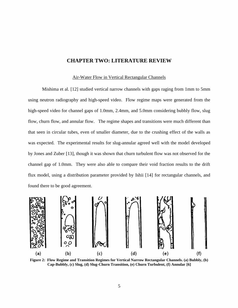
Hibiki and Mishima [16] developed models for flow regime transition for upward flow
through narrow channels and compared with the existing data for gaps ranging from .3mm to
17mm. The regimes considered were bubbly flow, slug flow, churn flow, and annular flow. For
bubble to slug, the transition occurred due to an increase in probability of bubble collisions,
related to bubble size compared to the size of the channel gap and the void fraction. This
occurred at a void fraction of 20% for bubbles larger than the narrow gap increasing up to 30%
for bubbles much smaller than the gap, which is comparable to that of larger channels of both
rectangular and circular cross section. The flow regime map for a gap size of 2.45mm from
Mishima et al. [12] can be seen below with transition lines from Hibiki and Mishima [16]
overlaid, showing good agreement between the model and experimental results.
7
Figure 3: Flow Regime Map and Transition Lines for a Narrow Rectangular Duct [12],[16]
Hot-Film Anemometer Signal Response in Multiphase Flow
A constant temperature hot-film anemometer works on the principle of responding to
differences in convection rates in a fluid flow. In single phase flows, this response is due to
changes in velocity of the phase, with higher momentum fluid convecting away more heat, and
requiring a higher power output to maintain the constant temperature. In multiphase
applications, the principal cause of response is due to the difference in the heat capacities of the
phases; however, any other causes of a convective difference in the flow will still be reflected in
the signal. Typically, the footprints of alternative effects are small compared to the differences
caused by the heat capacities, but they define the behavior in the transition zone surrounding the
passage of a phase bubble. The signal response of the bubble interacting with the sensor has
been studied in detail and is necessary in the understanding of the hot-film method.
8
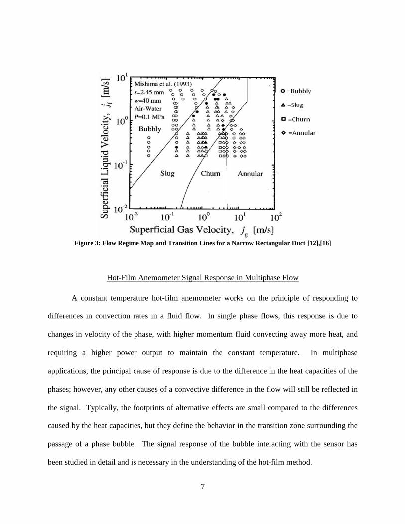
A typical signal response to a bubble passage is characterized by a slight rise in the signal
level as the bubble approaches, following a steep drop that smoothly approaches a low base
level, a sharp upwards spike, and then a smooth transition back down to the regular signal level
as the bubble drifts away. There is general agreement that the elevated signals preceding and
following the bubble are caused by the motion of the liquid rapidly being displaced by the
approaching volume. Bremhorst and Gilmore [17] studied the interaction at the phase interfaces
using controlled dipping style tests, and concluded that the steep drop and smooth transition at
the beginning was due to the exposure of the sensor to the gaseous phase, but with a thin liquid
meniscus remaining attached to the sensor portion, which thins as the probe pierces further into
the bubble. Further, they showed that the sharp spike at the end is due to a meniscus formation
at the tail of the bubble, in which the interface holds onto the bubble causing a stretching effect.
They concluded that the steep slope at the beginning of the interaction is to be included as a
portion of the bubble phase, but the sharp spike at the end is a detachment tail and should not be
included as portion of the natural bubble phase.
Figure 4: Typical Signal Response to Bubble Passage. A. Front interface, B. Rear interface, C. Detachment
tail collapse, D. Return to liquid phase [18]
9
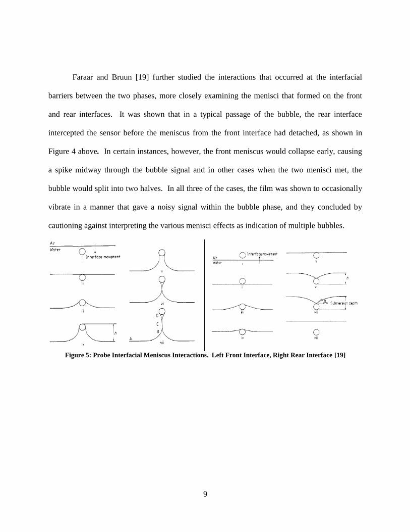
Faraar and Bruun [19] further studied the interactions that occurred at the interfacial
barriers between the two phases, more closely examining the menisci that formed on the front
and rear interfaces. It was shown that in a typical passage of the bubble, the rear interface
intercepted the sensor before the meniscus from the front interface had detached, as shown in
Figure 4 above. In certain instances, however, the front meniscus would collapse early, causing
a spike midway through the bubble signal and in other cases when the two menisci met, the
bubble would split into two halves. In all three of the cases, the film was shown to occasionally
vibrate in a manner that gave a noisy signal within the bubble phase, and they concluded by
cautioning against interpreting the various menisci effects as indication of multiple bubbles.
Figure 5: Probe Interfacial Meniscus Interactions. Left Front Interface, Right Rear Interface [19]
10
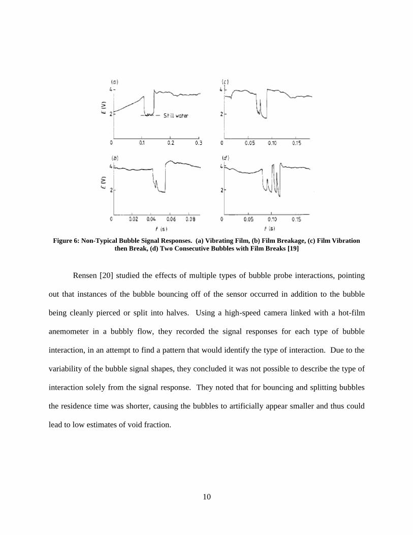
Figure 6: Non-Typical Bubble Signal Responses. (a) Vibrating Film, (b) Film Breakage, (c) Film Vibration
then Break, (d) Two Consecutive Bubbles with Film Breaks [19]
Rensen [20] studied the effects of multiple types of bubble probe interactions, pointing
out that instances of the bubble bouncing off of the sensor occurred in addition to the bubble
being cleanly pierced or split into halves. Using a high-speed camera linked with a hot-film
anemometer in a bubbly flow, they recorded the signal responses for each type of bubble
interaction, in an attempt to find a pattern that would identify the type of interaction. Due to the
variability of the bubble signal shapes, they concluded it was not possible to describe the type of
interaction solely from the signal response. They noted that for bouncing and splitting bubbles
the residence time was shorter, causing the bubbles to artificially appear smaller and thus could
lead to low estimates of void fraction.
11
Hot-Film Anemometer Signal Analysis
To obtain useful information from the hot-film anemometer signal when applied to
multiphase flow, it is necessary to be able to distinguish between the two phases. Toral [21]
describes a method by which the amplitude of the signal is the basis of discrimination, denoting
every voltage value above a threshold as the primary phase, and everything below it the
secondary phase. To determine the voltage threshold a histogram of the voltage data is created,
which reveals a bi-modal distribution. One peak refers to the most probable base voltage level of
the primary phase, and other to the most probable base voltage level of the secondary phase, and
a point between these two peaks is typically denoted as the threshold value. This specific point
selected is up to the judgment of the researcher, and a few methods of selection are employed.
Trabold et al. [22] recommends using the halfway point between the peaks, and Farrar et al. [18]
recommends the lowest point between the two peaks. A study by Resch [23] recommends
calculating the void fraction of the data for a range of threshold values, and then selecting the
point at which the void fraction is least affected by changes in the threshold. In order to obtain a
statistically signficant histogram for threshold selection, a sampling time of 1 to 3 minutes is
generally recommended [21].
Another prominent method of phase discrimination looks at the first-derivative of the
signal, noticing that a sharp negative spike occurs with the passage of the liquid-gas interface,
and that a sharp positive spike occurs with the passage of the gas-liquid interface. A slope-
threshold is then denoted based on the difference in voltage amplitude of the two-phases, and the
observed time it takes for the signal to fluctuate between the two voltage levels. When the
derivative of the signal passes the negative threshold, the beginning of the gas phase is noted,
12
and the signal is considered gaseous until the derivative passes the positive threshold. This
method was detailed by Farrar and Bruun [19]. Both of these basic methods have their
advantages and disadvantages, and are appropriate in different situations, discussed in length by
Farrar et al. [18].
Once the phases can be identified, it is useful to translate the data into a phase indication
form, setting all values associated with the liquid phase as 1 and all values associated with the
gaseous phase as 0. With this, various properties of the flow can be understood. The bubble
frequency is found from the number of bubbles, indicated by the passing of two interfaces,
experienced during the time of the experiment. For set ups employing two parallel sensors,
bubble speed can be found by the time shift of the interfaces being recognized between the two
signals, along with the known distance between the two sensors. With a known bubble speed, a
bubble streamwise length can be found from the time duration of the probe/bubble interaction.
These methods have been successfully described and employed with different details by [24]
[25], [26], and [27]. The specific methods employed for the purposes of the present research will
be discussed in further length in the Methodology section.
13
CHAPTER THREE: METHODOLOGY
Experimental Facility
Air-Water Test Loop Overview
An air-water test loop was created to maintain steady and controllable air and water flow
rates in order to simulate various bubbly flow conditions in a vertical acrylic test section. A
rotary vane type positive displacement pump (¼ HP, 1725 RPM) pumps water from a reservoir
through the entirety of the loop and back into its own reservoir. The flow rate is regulated by
two flow control valves, redirecting portions of the water back into the water reservoir before
entering the circuit. The liquid flow rate in the loop is measured by a 0-2 liters per minute
infrared paddle wheel turbine type flow meter. The air is delivered by a piston style air pump
(3.5 W, 60 Hz), and is injected into the vertical test section through a porous bubble stone. The
air flow rate is controlled by a needle valve, and measured by a 0-.5 liter per minute hot mesh
type air flow meter. A check valve is placed between the flow meter and the test section in order
to prevent water from backing up into the air line and compromising the sensitive hot-mesh
sensor. A thermocouple is placed in the line just before the loop dumps to the reservoir in order
to monitor the temperature of the water just coming past the hot-film sensor. The liquid flow
meter, air flow meter, and thermocouple data are read by modules on an NI cDAQ, recorded by a
custom LabView VI, and then saved in spreadsheet format for future reference.
All piping in the system is semi-transparent ¼” ID polyethylene tubing, other than the
1/16” vinyl air lines, and an 18” portion of ¼” copper tubing leading up the liquid flow meter, in
order to create a sufficiently developed flow for the flow meter to measure. A 2ft length of ½”

14
Schedule 80 transparent PVC is located just before the vertical test section, that allows for a
viewing of the flow, namely to ensure that no extraneous air is entrained in the flow preceding
the air input section. A mesh filter is placed before the control valves in order to collect any
particles that enter the flow that could be hazardous to the liquid flow meter or hot-film
anemometer probe. A schematic of the loop can be seen below in Figure 7.
Figure 7: Air-Water Test Loop Schematic
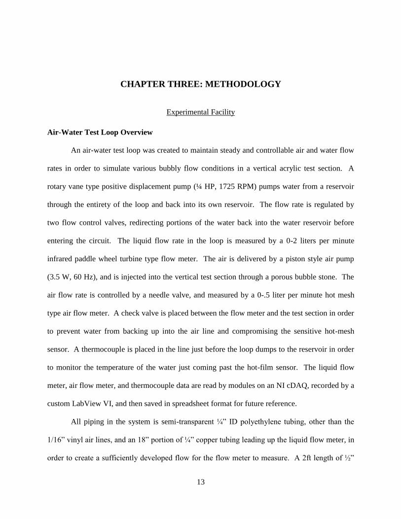
Vertical Test Section
The vertical test section consists of three pieces of acrylic glass held together by a series
of bolts. One section has the channel carved into it, along with the flow strengtheners at the
entrance, a smaller center section piece has a rubber seal inset into a groove surrounding the
channel, and the third section acts to sandwich the center section into the first section, creating
the seal.
15
Figure 8: Vertical Test Section Diagram
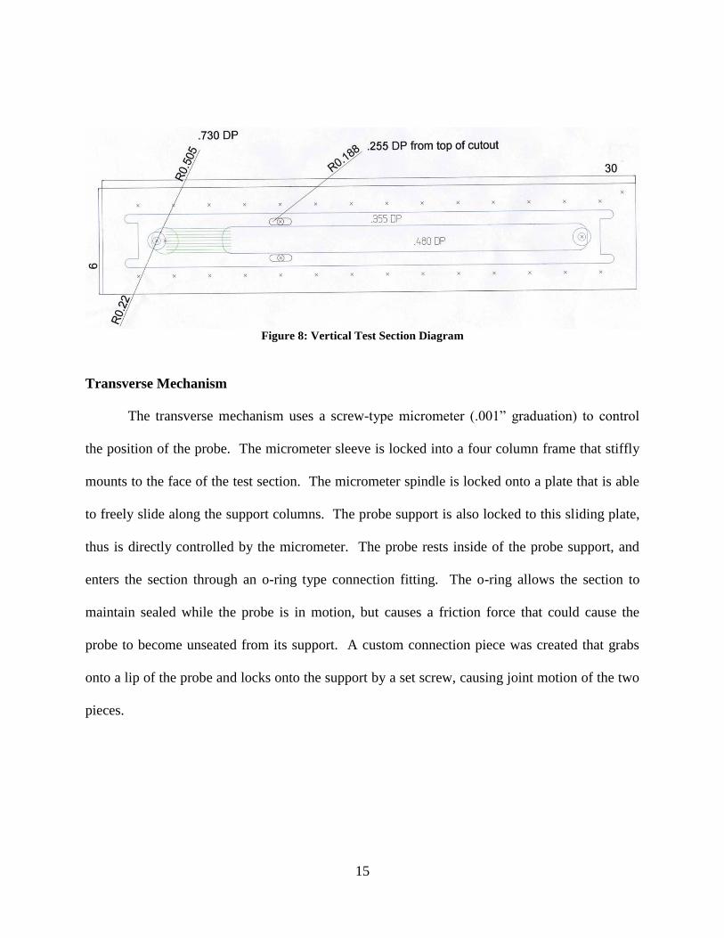
Transverse Mechanism
The transverse mechanism uses a screw-type micrometer (.001” graduation) to control
the position of the probe. The micrometer sleeve is locked into a four column frame that stiffly
mounts to the face of the test section. The micrometer spindle is locked onto a plate that is able
to freely slide along the support columns. The probe support is also locked to this sliding plate,
thus is directly controlled by the micrometer. The probe rests inside of the probe support, and
enters the section through an o-ring type connection fitting. The o-ring allows the section to
maintain sealed while the probe is in motion, but causes a friction force that could cause the
probe to become unseated from its support. A custom connection piece was created that grabs
onto a lip of the probe and locks onto the support by a set screw, causing joint motion of the two
pieces.
16
Figure 9: Transverse Mechanism Schematic
Any bending or twisting of the sliding plate would cause uncertainty in the location of the
probe in respect to the micrometer, so a 90 degree angle must be constantly maintained between
the plate and the support columns. To ensure the sliding plate remains strictly vertical, the
columns and plate were very tightly toleranced, requiring pre-lubricated bushings in the guide
holes to allow sliding to occur. Springs on each column maintain an even loading on the plate,
as any slight twisting motion will cause it to lock in place, unable to move. The columns
themselves rest inside counterbores on the support plate, rigidly maintaining themselves parallel
in respect to one another. These various measures and connection pieces ensure a smooth direct
one-to-one motion between the micrometer spindle and the probe sensor.
17
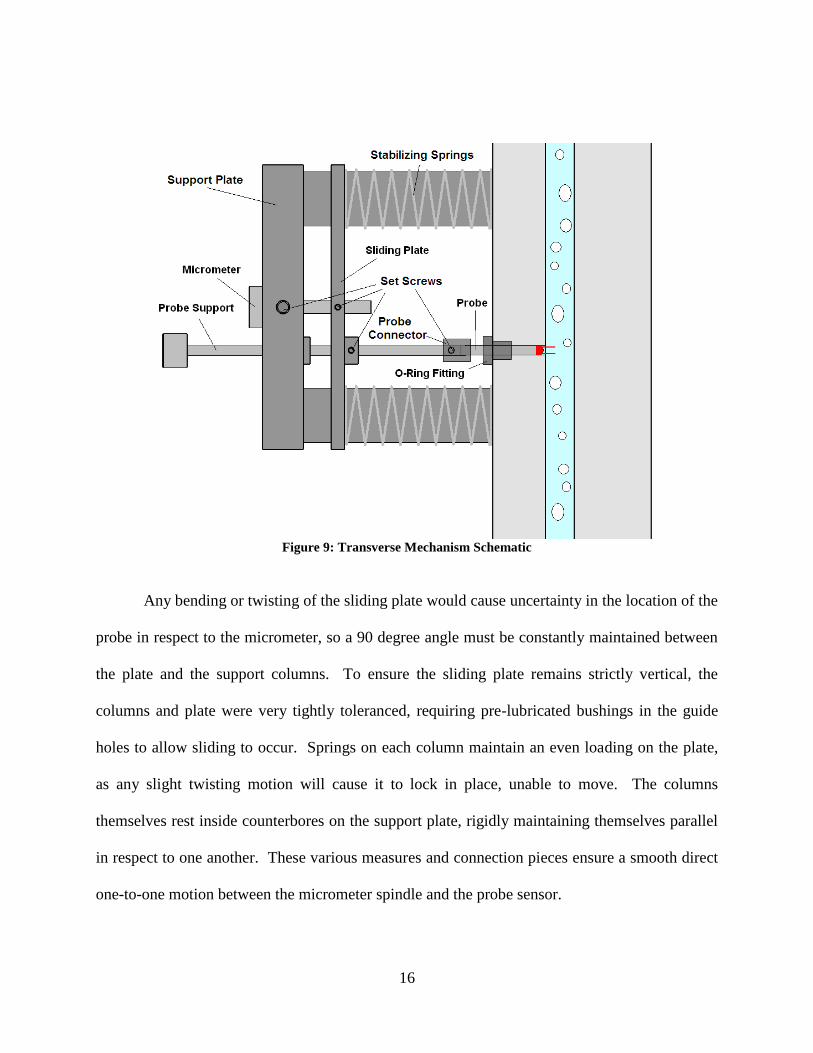
Figure 10: Photograph of the Transverse Mechanism
The mechanism was also designed to be flexible in its placement of the sensor. The four
columns are spaced such that they attach onto any four bolt holes that span along the height of
the test section. Further, grooves in the support plate and sliding plate allow the probe to be
shifted up and down within the area between the four bolt holes. The combination between bolt
hole selection and shifting of the probe allow the sensor to take measurements at any vertical
18
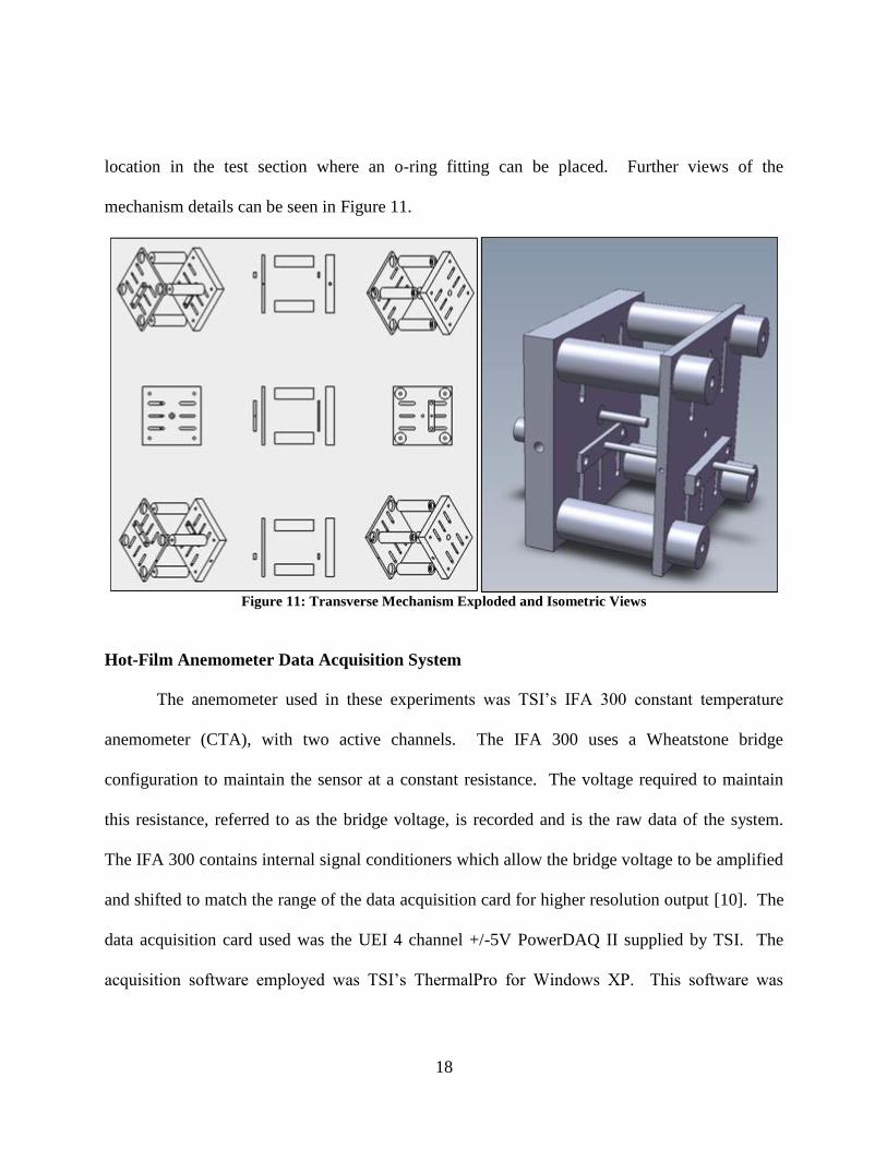
location in the test section where an o-ring fitting can be placed. Further views of the
mechanism details can be seen in Figure 11.
Figure 11: Transverse Mechanism Exploded and Isometric Views
Hot-Film Anemometer Data Acquisition System
The anemometer used in these experiments was TSI’s IFA 300 constant temperature
anemometer (CTA), with two active channels. The IFA 300 uses a Wheatstone bridge
configuration to maintain the sensor at a constant resistance. The voltage required to maintain
this resistance, referred to as the bridge voltage, is recorded and is the raw data of the system.
The IFA 300 contains internal signal conditioners which allow the bridge voltage to be amplified
and shifted to match the range of the data acquisition card for higher resolution output [10]. The
data acquisition card used was the UEI 4 channel +/-5V PowerDAQ II supplied by TSI. The
acquisition software employed was TSI’s ThermalPro for Windows XP. This software was
19
responsible for setting the operating conditions of the probe, configuring the sampling conditions
for data acquisition, triggering the anemometer, and recording the voltage data.
TSI’s 1244-20W hot film probe was used for the purposes of this research, which
consists of two platinum coated quartz tube (50.8μm dia) sensors in a parallel alignment. The
sensors have a 1.02 mm sensing length, and are at a distance of 1.016 mm in the streamwise
direction. Each sensor on the probe occupies its own channel on the IFA 300 cabinet and A/D
converter board.
High Speed Camera
The high speed camera employed was a Fastec Troubleshooter (model: TSHRMM),
which contains a CMOS array, and records up to a resolution of 1280 x 1024 pixels, with 8-bit
pixel resolution in monochrome and 24-bit pixel resolution in color. The Troubleshooter is a
standalone device containing its own data storage device (3GB), and a display for viewing and
editing footage directly after recording. The camera was mounted on a tripod, facing the
opposite side of the channel from which the transverse mechanism was mounted to obtain a clear
view of the flow. A blank piece of white poster board was placed behind the channel to offer a
solid background, at a distance far enough away such that shadows would not be cast on it. A
function generator was used for external triggering, to avoid handling of the camera which could
cause motion during recording or resetting of the camera position. Two 27W (120 V 60Hz)
compact fluorescent lamps were used for lighting, positioned above and below the area of
interest to shed a blanket of even lighting. Though the recording frequency was greater than the
20
frequency of the AC bulbs, the flickering was found to have minimal effect due to the quality of
the backdrop and the strength of image processing system.
HFA Signal Analysis
Phase Discrimination and Void Fraction
For the purpose of signal slope based phase discrimination, a program was generated that
would crawl through the first derivative of the signal, looking for spikes that reached the slope
threshold in both the negative and positive directions, signifying the arrival or passage of a
bubble respectively. When the spike was negative, this was considered to be the result of the
signal transitioning from the liquid phase to the gaseous phase. In this case, the program would
back up through the data looking for the derivative of the signal to switch to positive, signifying
the instant the sensor came into contact with the front edge of the bubble, and then would crawl
forward looking for a second point where the derivative of the signal again switched to positive,
signifying the instant the sensor came into contact with the rear edge of the bubble. This portion
between the two sign changes was denoted as 0’s in the phase indicator, indicating the gaseous
phase. A similar scenario occurred when the program came across a positive spike, instead
working in the reverse, finding the rear edge of the bubble, and crawling back to the front edge.
The exact transition of negative to positive slope was actually selected by the slope reaching a
value of positive ten, to avoid false triggers due to small noisy voltage fluctuations occurring in
the low slope portion of the bubble, as suggested by [18]. The hybrid method was triggered by
the signal dipping below the amplitude threshold value, and again following a similar pattern as
the slope method to adjust the edges of the bubble interaction. Upon the trigger, the program
would first walk backwards through the signal until the slope of the signal reach the value of
21
positive ten, as was previously done to denote the beginning of the bubble. The program would
then go back to the instance of crossing the amplitude threshold and then continue until it came
back above this threshold, as the signal approached the normal liquid voltage level. This point
does not actually correspond to the edge of the bubble, so it would again crawl backwards until
the slope reached a value of negative ten, to indicate the point at the which signal started
increasing upon the sensor first touching liquid. The program would then go back the second
triggering event to crawl forward looking for more triggers, as to not be triggered by the same
point.
The selection of the trigger threshold was a unique method based on the method
employed by [23] for selecting an amplitude threshold, in which the void fraction was calculated
for a range of amplitude threshold values, and the threshold being selected by the shape of the
resulting curve. In this case, it was applied to the slope threshold as well, calculating the void
fraction for various values and the appropriate threshold was taken from the features in the curve.
What is unique in this study was differentiating the void fraction vs slope threshold curve in
order to reveal further features.
Void Fraction
To calculate the local void fraction, the number of points listed as 0 in the phase indicator
were counted, and divided by the total number of points in the sample. For the non-local void
fraction, data sets were taken for various points across the channel, and the local void fractions
were then integrated across the area of the channel using a Trapezoidal Riemann Sum method.

22
Bubble Speed
A discrete, normalized cross-correlation function was used to find the most probable
time-shift of the bubble passages between the two parallel sensors. Because the sensors run at
different operating resistances, due to the inherent uniqueness of any hot-film sensor, the signals
occur across different voltage ranges, and thus the exact signal amplitudes are not comparable.
To help the correlation, the signals are first normalized by subtraction the mean, and dividing by
the standard deviation. The correlation function then integrates the product of the normalized
signal of the first sensor and the normalized time-shifted signal of the second sensor over the
entire data set. This integration is done for a range of time-shifts, and the time-shift that yields
the highest correlation is selected as the average time taken for a bubble interface to pass
between both sensors. The bubble speed is then calculated from the time taken to pass between
sensors, and the known distance between the sensors. It is also not trivial to again point out that
this cross correlation was applied directly to the normalized voltage signals, and not to the phase
indicator function. In some instances researchers employing the cross-correlation method choose
to run the correlation for the phase indicator function, but in the present case it was found that
the signal of the downstream sensor was not ideal for the generation of its own phase indication
function. This is the method successfully employed by van der Welle [26], Wang-Ching [27],
and [28]. The normalized cross correlation function used in this case can be seen in Equation 1.
totT
tot
dttVtV
TR
0 21
2211 ))(())((1)(
totT
ttot
tVtV
TR
0 21
2211 ))(())((1)(
Equation 1: Normalized Cross Correlation Function for Most Probable Interfacial Time-shift
23
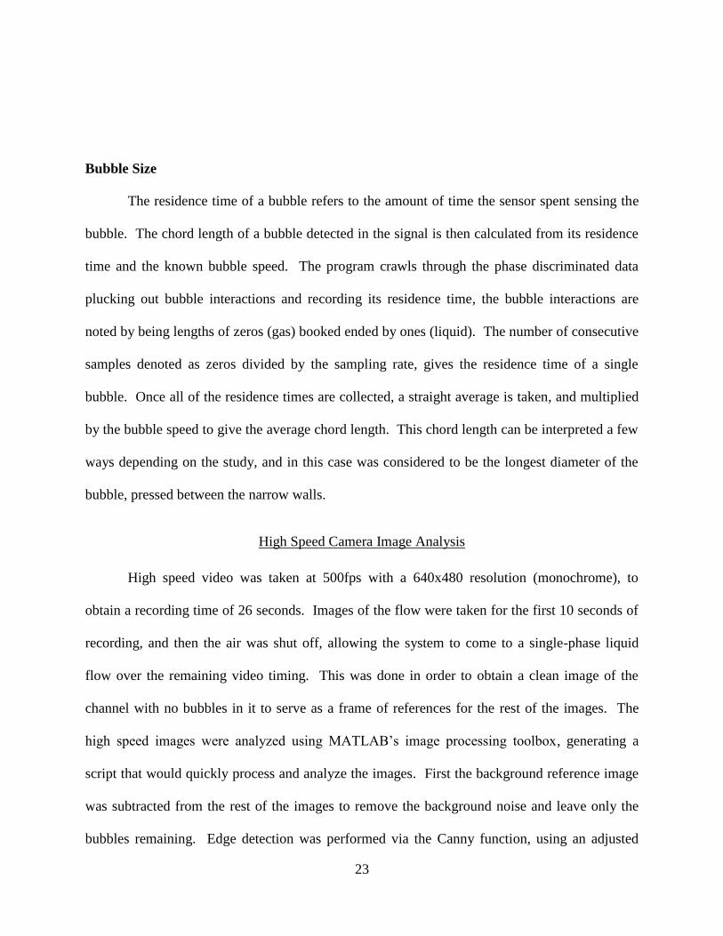
Bubble Size
The residence time of a bubble refers to the amount of time the sensor spent sensing the
bubble. The chord length of a bubble detected in the signal is then calculated from its residence
time and the known bubble speed. The program crawls through the phase discriminated data
plucking out bubble interactions and recording its residence time, the bubble interactions are
noted by being lengths of zeros (gas) booked ended by ones (liquid). The number of consecutive
samples denoted as zeros divided by the sampling rate, gives the residence time of a single
bubble. Once all of the residence times are collected, a straight average is taken, and multiplied
by the bubble speed to give the average chord length. This chord length can be interpreted a few
ways depending on the study, and in this case was considered to be the longest diameter of the
bubble, pressed between the narrow walls.
High Speed Camera Image Analysis
High speed video was taken at 500fps with a 640x480 resolution (monochrome), to
obtain a recording time of 26 seconds. Images of the flow were taken for the first 10 seconds of
recording, and then the air was shut off, allowing the system to come to a single-phase liquid
flow over the remaining video timing. This was done in order to obtain a clean image of the
channel with no bubbles in it to serve as a frame of references for the rest of the images. The
high speed images were analyzed using MATLAB’s image processing toolbox, generating a
script that would quickly process and analyze the images. First the background reference image
was subtracted from the rest of the images to remove the background noise and leave only the
bubbles remaining. Edge detection was performed via the Canny function, using an adjusted

24
threshold to further remove noise. The Canny function employs two thresholds, one major
threshold to find any strong edges, and a second minor threshold to find any weak edges that are
touching any strong edges to connect the outline of the object with no gaps [29]. Each bubble
outline was then filled in to mark each bubble as a clear single object in the image. The script
would label each object found in the image, and then would provide information about each
object, such as the centroid location, area, and dimensions. The image could then be displayed
with each object given a distinct color, to give a quick look at the labeling. This color labeling
was important in the velocity analysis, which made it possible to quickly check that a bubble
maintained the same label through two consecutive images, following a left-to-right labeling
order.
Figure 12: Image Processing Technique
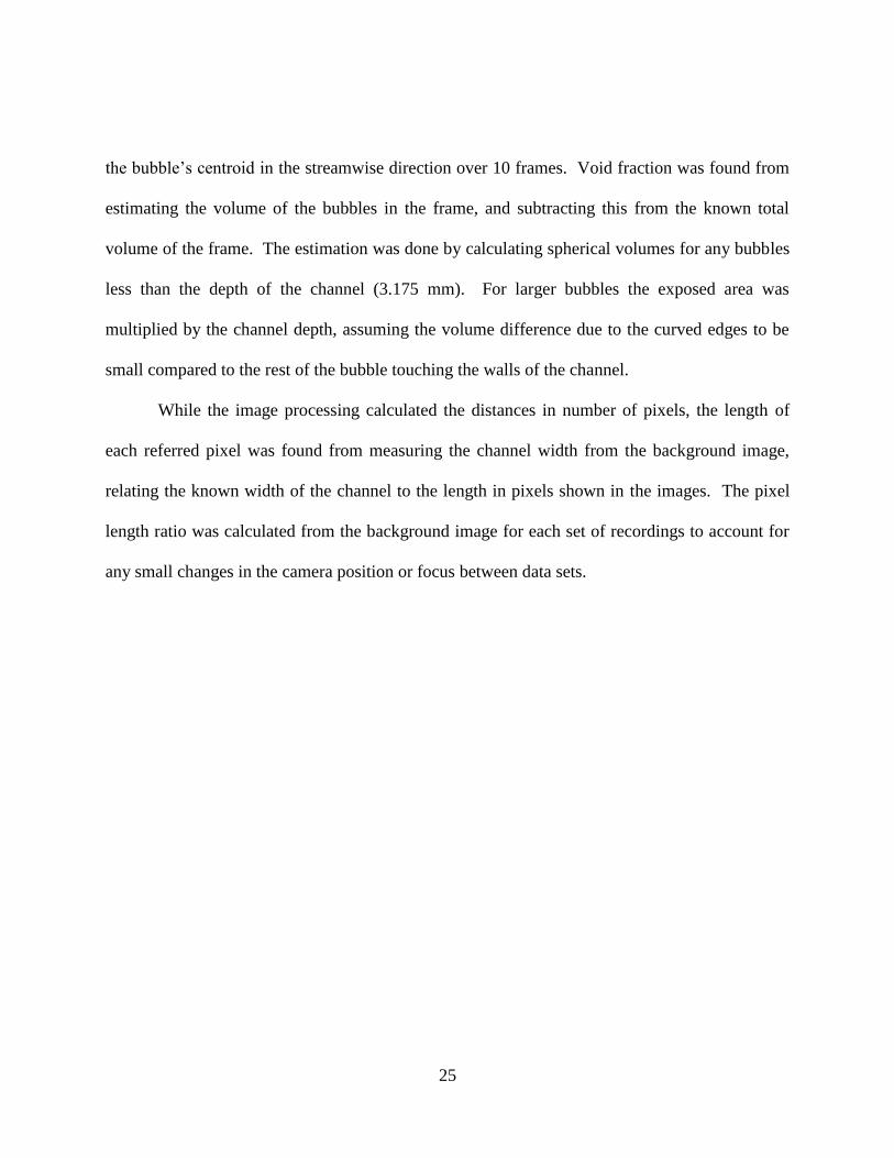
The bubble diameter was taken as the diameter of the circle with an area equal to the area
of the somewhat irregularly shaped bubble. The velocity was taken as the change in location of
25
the bubble’s centroid in the streamwise direction over 10 frames. Void fraction was found from
estimating the volume of the bubbles in the frame, and subtracting this from the known total
volume of the frame. The estimation was done by calculating spherical volumes for any bubbles
less than the depth of the channel (3.175 mm). For larger bubbles the exposed area was
multiplied by the channel depth, assuming the volume difference due to the curved edges to be
small compared to the rest of the bubble touching the walls of the channel.
While the image processing calculated the distances in number of pixels, the length of
each referred pixel was found from measuring the channel width from the background image,
relating the known width of the channel to the length in pixels shown in the images. The pixel
length ratio was calculated from the background image for each set of recordings to account for
any small changes in the camera position or focus between data sets.

26
CHAPTER FOUR: RESULTS AND DISCUSSION
Cases Run
Tests were performed for different superficial liquid and gas velocities to obtain varying
flow volume fractions. The parameters were chosen based on the ranges that stayed within the
boundary of bubbly flow regime, as provided by Mishima’s flow regime maps for rectangular
channels with 2.4 mm and 5.0 mm gaps [12]. The range of velocities and subsequent volume
fractions examined can be seen below.
Table 1: Test Matrix
Test #
Q-l (L/min)
Q-g (L/min)
j-l (m/s)
j-g (m/s)
j (m/s)
Volume Fraction
61 1.336 0.030 0.184 0.004 0.188 0.022
62 0.980 0.031 0.135 0.004 0.139 0.030
60 1.333 0.081 0.184 0.011 0.195 0.057
68 1.030 0.084 0.142 0.012 0.154 0.076
49 1.179 0.100 0.162 0.014 0.176 0.078
50 0.981 0.084 0.135 0.012 0.147 0.079
30 0.980 0.084 0.135 0.012 0.147 0.079
39 1.031 0.103 0.142 0.014 0.156 0.091
28 0.978 0.102 0.135 0.014 0.149 0.094
45 0.981 0.102 0.135 0.014 0.149 0.094
48 1.233 0.129 0.170 0.018 0.188 0.095
37 1.082 0.129 0.149 0.018 0.167 0.107
32 1.080 0.129 0.149 0.018 0.167 0.107
44 1.031 0.129 0.142 0.018 0.160 0.111
38 1.029 0.130 0.142 0.018 0.160 0.112
46 1.277 0.163 0.176 0.022 0.198 0.113
34 0.977 0.128 0.135 0.018 0.152 0.116
36 0.984 0.129 0.136 0.018 0.153 0.116
35 0.976 0.129 0.134 0.018 0.152 0.117
33 0.984 0.132 0.136 0.018 0.154 0.118
29 0.980 0.134 0.135 0.019 0.154 0.121
52 1.127 0.162 0.155 0.022 0.178 0.126
47 1.329 0.193 0.183 0.027 0.210 0.127
42 1.080 0.161 0.149 0.022 0.171 0.130
40 1.031 0.162 0.142 0.022 0.164 0.136

27
51 1.185 0.193 0.163 0.027 0.190 0.140
53 1.130 0.194 0.156 0.027 0.182 0.147
43 1.080 0.193 0.149 0.027 0.175 0.152
31 1.080 0.193 0.149 0.027 0.175 0.152
63 1.077 0.193 0.148 0.027 0.175 0.152
67 1.032 0.190 0.142 0.026 0.168 0.155
54 0.980 0.197 0.135 0.027 0.162 0.167
58 1.328 0.296 0.183 0.041 0.224 0.182
56 0.975 0.255 0.134 0.035 0.169 0.207
66 1.033 0.307 0.142 0.042 0.185 0.229
59 1.139 0.372 0.157 0.051 0.208 0.246
64 1.036 0.431 0.143 0.059 0.202 0.294
57 0.957 0.439 0.132 0.060 0.192 0.314
65 0.957 0.521 0.132 0.072 0.204 0.353
D ata R ang e
0.130
0.140
0.150
0.160
0.170
0.180
0.190
0.200
0.000 0.010 0.020 0.030 0.040 0.050 0.060 0.070 0.080
Superficial Gas Velocity (m/s)
Su
perf
icia
l L
iqu
id V
elo
cit
y (
m/s
)
C AM H F A
Figure 13: Map of Superficial Liquid and Gas Velocities Examined
Some sample images from the high-speed video results can be seen below, illustrating the
wide-range in bubbly flow regimes studied.

28
Figure 14: Sample Images from Volume Fraction of 2.2%
Figure 15: Sample Images from Volume Fraction of 15.2%
Figure 16: Sample Images from Volume Fraction of 35.3%
29
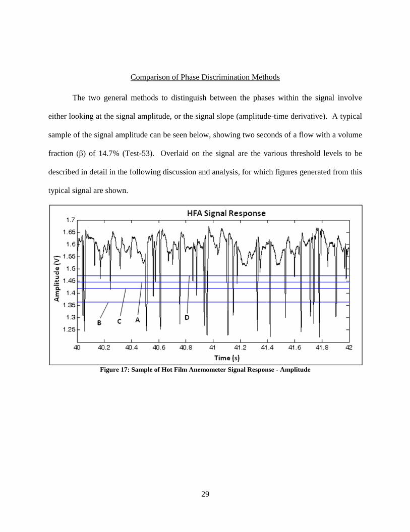
Comparison of Phase Discrimination Methods
The two general methods to distinguish between the phases within the signal involve
either looking at the signal amplitude, or the signal slope (amplitude-time derivative). A typical
sample of the signal amplitude can be seen below, showing two seconds of a flow with a volume
fraction (β) of 14.7% (Test-53). Overlaid on the signal are the various threshold levels to be
described in detail in the following discussion and analysis, for which figures generated from this
typical signal are shown.
Figure 17: Sample of Hot Film Anemometer Signal Response - Amplitude

30
Figure 18: Sample of Hot Film Anemometer Signal Response – Slope
The first thing that is commonly looked at for an amplitude threshold value is the voltage
histogram which shows two peaks, one corresponding to the most common gaseous phase
voltage, and one for the most common liquid phase voltage. The area between is an overlap
between the two phases, so a common and basic threshold value taken from this is the point
halfway between the peaks, which will be considered here.

31
Amplitude (V)
Fre
qu
en
cy
Voltage Histogram
Peak 1
Peak 2
Halfway
Between
Peaks
Amplitude (V)
Fre
qu
en
cy
Voltage Histogram
Peak 1
Peak 2
Halfway
Between
Peaks
Figure 19: Amplitude Threshold Selection - Voltage Histogram
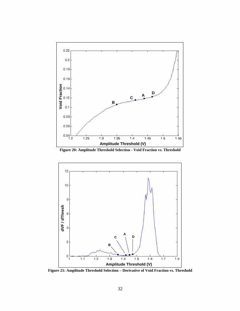
After running the code for the hybrid method of phase discrimination for a wide variety
of threshold values, a few patterns and points of interest appeared. The typical resulting curves
can be seen below detailing these points. Figure 20 shows that by increasing the threshold from
the minimum voltage in the signal all the way to the maximum voltage the void fraction can
range from zero to one. By looking at this derivative of this curve, shown in Figure 21, it is
apparent that the derivative resembles the voltage histogram due to the nature of amplitude phase
discrimination. The point shown as point A, is the point halfway between the peaks of the
voltage histogram seen in Figure 19. Points B and D refer to the limits of the flat area between
the two peaks, giving the most conservative and liberal estimations of threshold value that could
be made. Point C is the lowest value of the derivative within the trough, which would be an
inflection point and the point at which the void fraction changes the least due to changing
threshold value. Though this point seems to be near the centered between B and D, it is often off
to one side or the other depending on the nature of the peaks.
32
A
BC
D
Amplitude Threshold (V)
Vo
id F
rac
tio
n
A
BC
D
Amplitude Threshold (V)
Vo
id F
rac
tio
n
Figure 20: Amplitude Threshold Selection - Void Fraction vs. Threshold
Amplitude Threshold (V)
dV
F /
dT
hre
sh
A
B
C D
Amplitude Threshold (V)
dV
F /
dT
hre
sh
A
B
C D
Figure 21: Amplitude Threshold Selection – Derivative of Void Fraction vs. Threshold
33
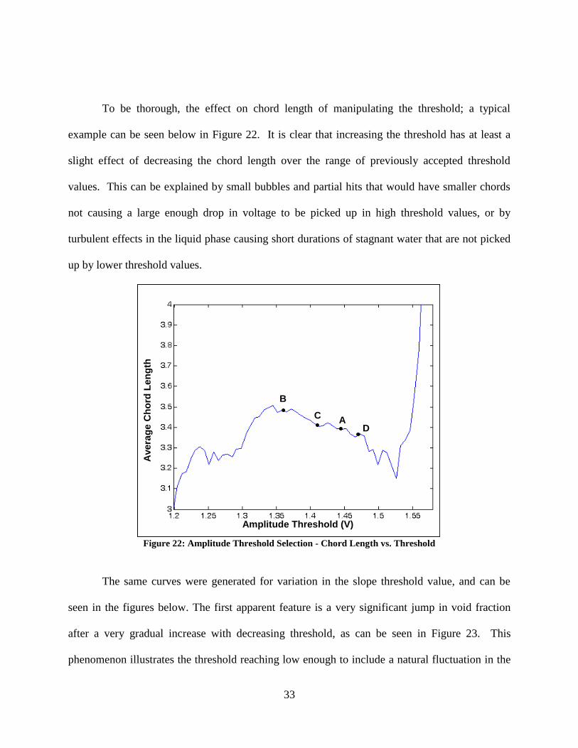
To be thorough, the effect on chord length of manipulating the threshold; a typical
example can be seen below in Figure 22. It is clear that increasing the threshold has at least a
slight effect of decreasing the chord length over the range of previously accepted threshold
values. This can be explained by small bubbles and partial hits that would have smaller chords
not causing a large enough drop in voltage to be picked up in high threshold values, or by
turbulent effects in the liquid phase causing short durations of stagnant water that are not picked
up by lower threshold values.
A
B
C
D
Amplitude Threshold (V)
Ave
rag
e C
ho
rd L
en
gth
A
B
C
D
Amplitude Threshold (V)
Ave
rag
e C
ho
rd L
en
gth
Figure 22: Amplitude Threshold Selection - Chord Length vs. Threshold
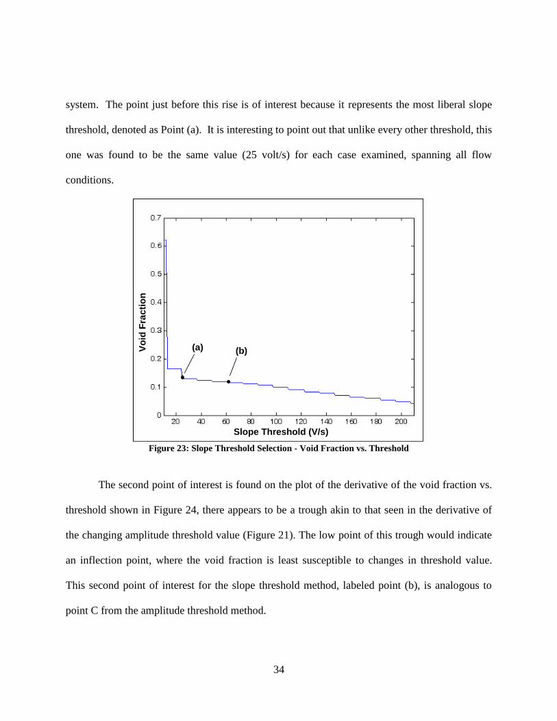
The same curves were generated for variation in the slope threshold value, and can be
seen in the figures below. The first apparent feature is a very significant jump in void fraction
after a very gradual increase with decreasing threshold, as can be seen in Figure 23. This
phenomenon illustrates the threshold reaching low enough to include a natural fluctuation in the
34
system. The point just before this rise is of interest because it represents the most liberal slope
threshold, denoted as Point (a). It is interesting to point out that unlike every other threshold, this
one was found to be the same value (25 volt/s) for each case examined, spanning all flow
conditions.
Slope Threshold (V/s)
Vo
id F
rac
tio
n
(a) (b)
Slope Threshold (V/s)
Vo
id F
rac
tio
n
(a) (b)
Figure 23: Slope Threshold Selection - Void Fraction vs. Threshold
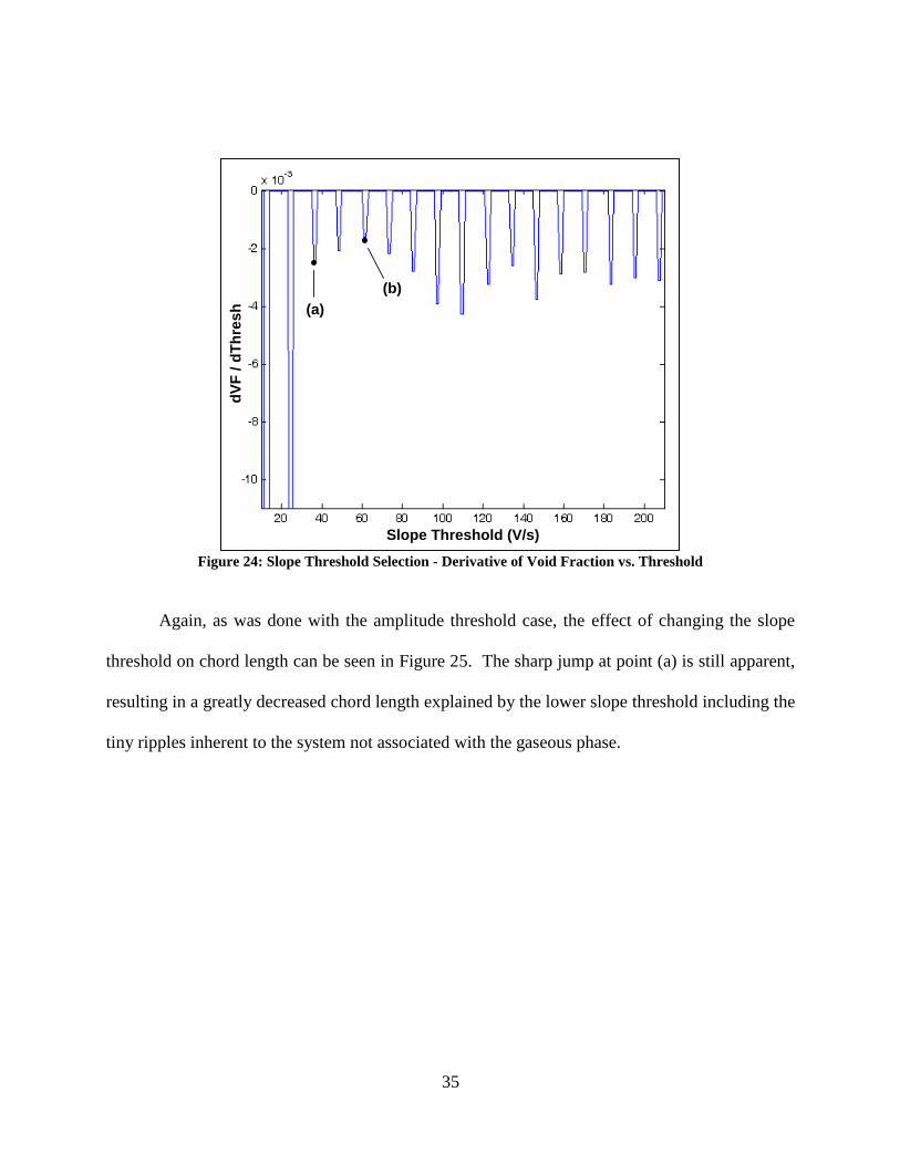
The second point of interest is found on the plot of the derivative of the void fraction vs.
threshold shown in Figure 24, there appears to be a trough akin to that seen in the derivative of
the changing amplitude threshold value (Figure 21). The low point of this trough would indicate
an inflection point, where the void fraction is least susceptible to changes in threshold value.
This second point of interest for the slope threshold method, labeled point (b), is analogous to
point C from the amplitude threshold method.
35
Slope Threshold (V/s)
dV
F /
dT
hre
sh (a)
(b)
Slope Threshold (V/s)
dV
F /
dT
hre
sh (a)
(b)
Figure 24: Slope Threshold Selection - Derivative of Void Fraction vs. Threshold
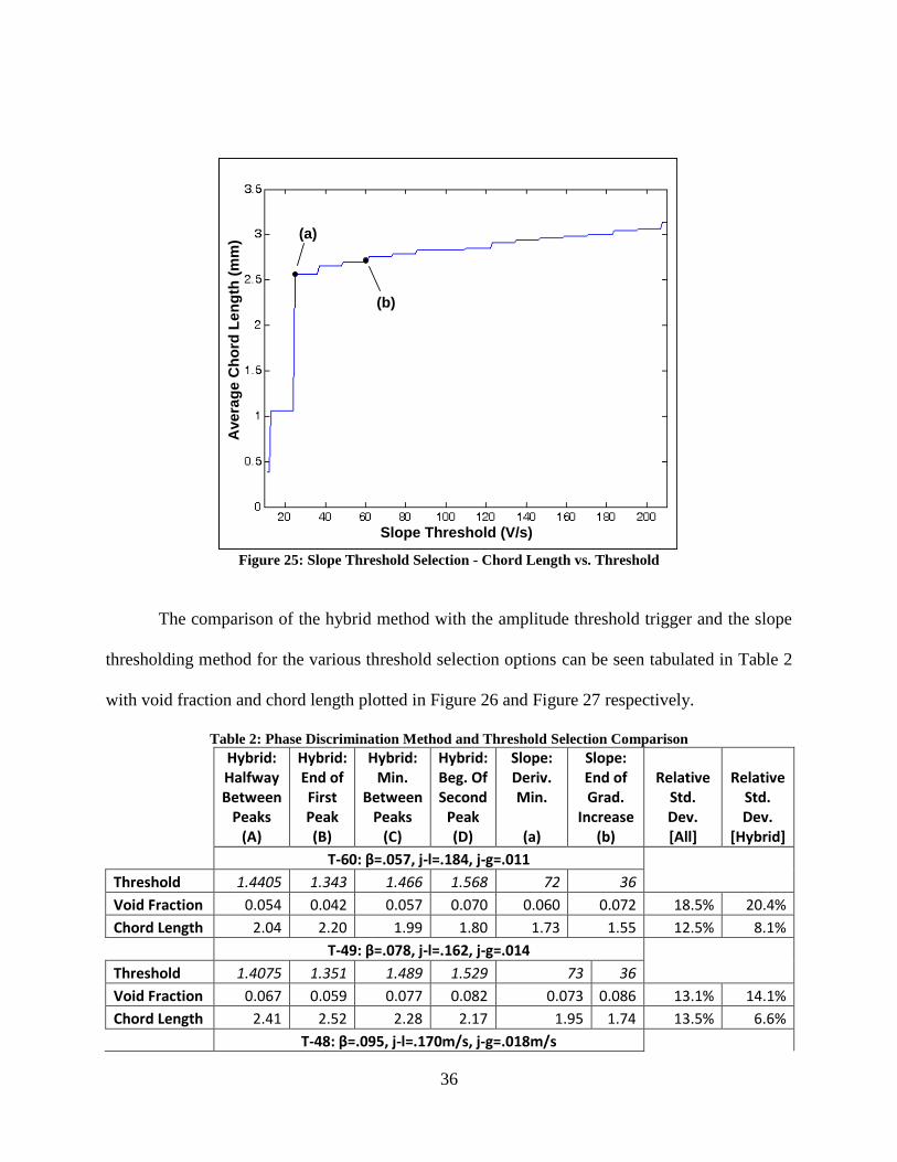
Again, as was done with the amplitude threshold case, the effect of changing the slope
threshold on chord length can be seen in Figure 25. The sharp jump at point (a) is still apparent,
resulting in a greatly decreased chord length explained by the lower slope threshold including the
tiny ripples inherent to the system not associated with the gaseous phase.
36
Slope Threshold (V/s)
Ave
rag
e C
ho
rd L
en
gth
(m
m) (a)
(b)
Slope Threshold (V/s)
Ave
rag
e C
ho
rd L
en
gth
(m
m) (a)
(b)
Figure 25: Slope Threshold Selection - Chord Length vs. Threshold
The comparison of the hybrid method with the amplitude threshold trigger and the slope
thresholding method for the various threshold selection options can be seen tabulated in Table 2
with void fraction and chord length plotted in Figure 26 and Figure 27 respectively.
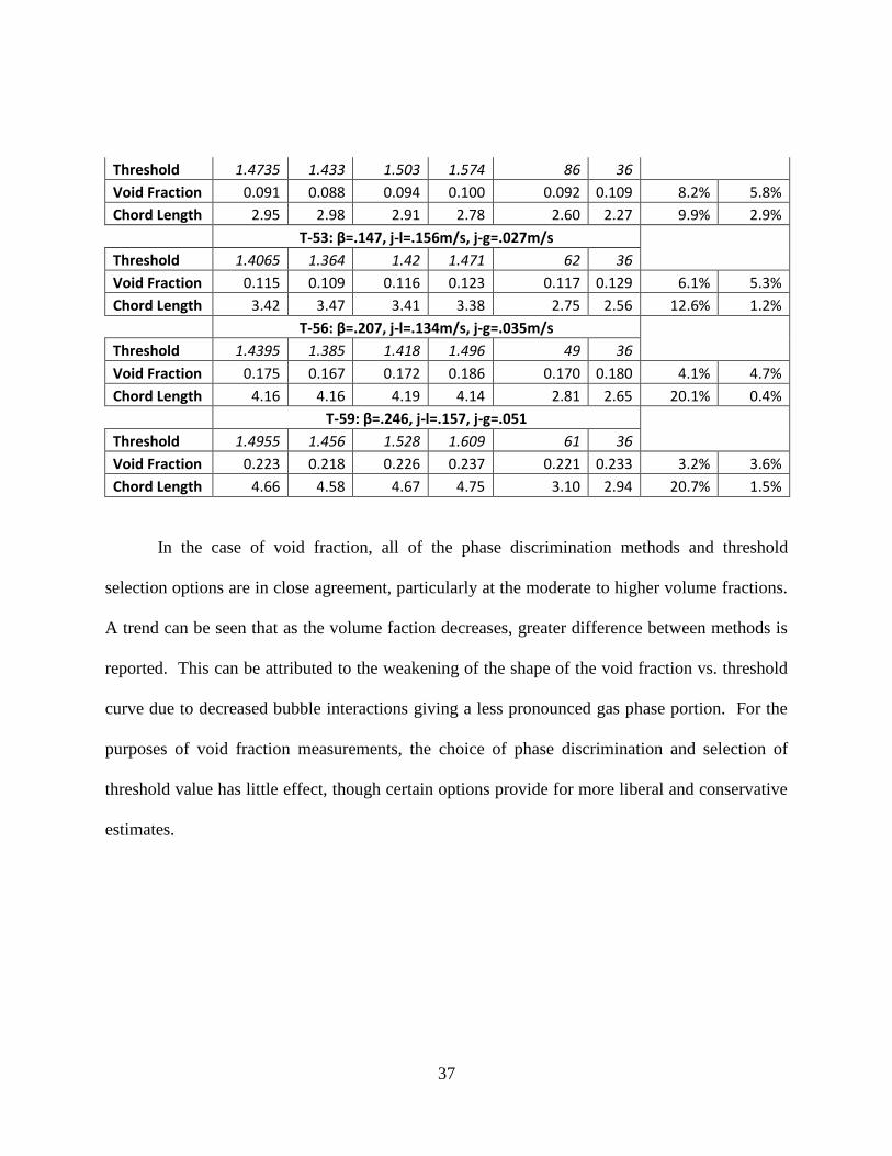
Table 2: Phase Discrimination Method and Threshold Selection Comparison
Hybrid: Halfway Between
Peaks (A)
Hybrid: End of First Peak (B)
Hybrid: Min.
Between Peaks
(C)
Hybrid: Beg. Of Second
Peak (D)
Slope: Deriv. Min.
(a)
Slope: End of Grad.
Increase (b)
Relative Std. Dev. [All]
Relative Std. Dev.
[Hybrid]
T-60: β=.057, j-l=.184, j-g=.011
Threshold 1.4405 1.343 1.466 1.568 72 36
Void Fraction 0.054 0.042 0.057 0.070 0.060 0.072 18.5% 20.4%
Chord Length 2.04 2.20 1.99 1.80 1.73 1.55 12.5% 8.1%
T-49: β=.078, j-l=.162, j-g=.014
Threshold 1.4075 1.351 1.489 1.529 73 36
Void Fraction 0.067 0.059 0.077 0.082 0.073 0.086 13.1% 14.1%
Chord Length 2.41 2.52 2.28 2.17 1.95 1.74 13.5% 6.6%
T-48: β=.095, j-l=.170m/s, j-g=.018m/s
37
Threshold 1.4735 1.433 1.503 1.574 86 36
Void Fraction 0.091 0.088 0.094 0.100 0.092 0.109 8.2% 5.8%
Chord Length 2.95 2.98 2.91 2.78 2.60 2.27 9.9% 2.9%
T-53: β=.147, j-l=.156m/s, j-g=.027m/s
Threshold 1.4065 1.364 1.42 1.471 62 36
Void Fraction 0.115 0.109 0.116 0.123 0.117 0.129 6.1% 5.3%
Chord Length 3.42 3.47 3.41 3.38 2.75 2.56 12.6% 1.2%
T-56: β=.207, j-l=.134m/s, j-g=.035m/s
Threshold 1.4395 1.385 1.418 1.496 49 36
Void Fraction 0.175 0.167 0.172 0.186 0.170 0.180 4.1% 4.7%
Chord Length 4.16 4.16 4.19 4.14 2.81 2.65 20.1% 0.4%
T-59: β=.246, j-l=.157, j-g=.051
Threshold 1.4955 1.456 1.528 1.609 61 36
Void Fraction 0.223 0.218 0.226 0.237 0.221 0.233 3.2% 3.6%
Chord Length 4.66 4.58 4.67 4.75 3.10 2.94 20.7% 1.5%
In the case of void fraction, all of the phase discrimination methods and threshold
selection options are in close agreement, particularly at the moderate to higher volume fractions.
A trend can be seen that as the volume faction decreases, greater difference between methods is
reported. This can be attributed to the weakening of the shape of the void fraction vs. threshold
curve due to decreased bubble interactions giving a less pronounced gas phase portion. For the
purposes of void fraction measurements, the choice of phase discrimination and selection of
threshold value has little effect, though certain options provide for more liberal and conservative
estimates.

38
Figure 26: Threshold Selection Comparison - Void Fraction
The chord length results, however, show a large deviation for the slope based phase
discrimination method. The tendency is for the chord lengths to be underestimated compared to
the results for the hybrid method. Because the slope method indicates little to no change in
chord length between volume fractions β=.095 and β=.246, it can be understood that the results
using this technique are unfavorable for these testing purposes.

39
Figure 27: Phase Discrimination Method and Threshold Selection Comparison
The proper phase discrimination technique for the purpose of this study would then come
down to a choice between the amplitude threshold selections using the hybrid technique. Being
that they are in close agreement, for both void fraction and chord length, the choice is a matter of
preference. The minimum in the trough of the void fraction vs. threshold derivative (point B)
lends itself as being distinctly identified and having roots in physical principles as an inflection
point where the bias of the liquid phase just begins to show an effect. The rest of the HFA
results reported in this study come from the hybrid phase discrimination technique with the
amplitude threshold being selected as the low point of the trough resulting from the
differentiating the plot of void fraction vs. threshold.

40
Void Fraction
To compare the results of these tests, the drift flux model was used based on Ishii’s
parameters as applied to rectangular channels [14]. This model with the distribution parameter
provided by Ishii can be seen in Equation 2. The ‘j’ refers to the superficial velocities, ‘s’ is the
narrow gap size (3.125mm), ‘w’ is the channel width (38.2mm), ‘g’ is the acceleration due to
gravity, and ‘ρ’ is the density of each phase.
llg
g
gwwsjjC
j
/)/13.23(.)(0
lgC /35.35.10
Equation 2: Drift Flux Model and Distribution Parameter for Rectangular Channels [14]
While some models predict void fraction (α) from volume fraction (β) by assuming a
constant slippage ratio, the drift flux model accounts for variation in superficial velocities. So
two cases with the same volume fraction can have somewhat different predicted void fractions
based on the total mixture volumetric flux (superficial liquid velocity + superficial gas velocity).
Volume fractions with a larger mixture volumetric flux will have a larger void fraction, due to
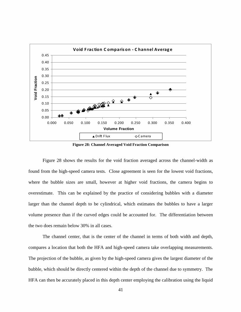
less slip occurring between the phases. This is apparent in Figure 28 as the predicted values of
void fraction by the correlation do not follow a strict linear relationship with the volume fraction,
due to variations in the mixture volumetric flux.
41
Void F rac tion C omparis on - C hannel Averag e
0.00
0.05
0.10
0.15
0.20
0.25
0.30
0.35
0.40
0.45
0.000 0.050 0.100 0.150 0.200 0.250 0.300 0.350 0.400
Volume Fraction
Vo
id F
racti
on
Drift F lux C amera
Figure 28: Channel Averaged Void Fraction Comparison
Figure 28 shows the results for the void fraction averaged across the channel-width as
found from the high-speed camera tests. Close agreement is seen for the lowest void fractions,
where the bubble sizes are small, however at higher void fractions, the camera begins to
overestimate. This can be explained by the practice of considering bubbles with a diameter
larger than the channel depth to be cylindrical, which estimates the bubbles to have a larger
volume presence than if the curved edges could be accounted for. The differentiation between
the two does remain below 30% in all cases.
The channel center, that is the center of the channel in terms of both width and depth,
compares a location that both the HFA and high-speed camera take overlapping measurements.
The projection of the bubble, as given by the high-speed camera gives the largest diameter of the
bubble, which should be directly centered within the depth of the channel due to symmetry. The
HFA can then be accurately placed in this depth center employing the calibration using the liquid
42
velocity profile as shown in Appendix A. Using this location the void fraction, bubble velocity,
and bubble diameter can be directly compared between the two methods.
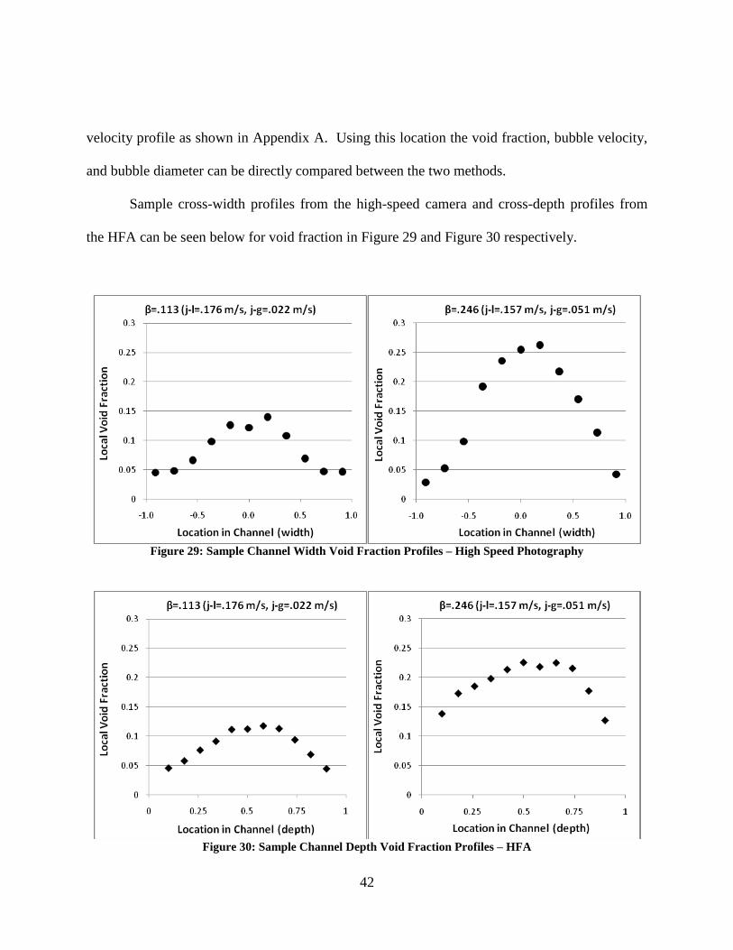
Sample cross-width profiles from the high-speed camera and cross-depth profiles from
the HFA can be seen below for void fraction in Figure 29 and Figure 30 respectively.
Figure 29: Sample Channel Width Void Fraction Profiles – High Speed Photography
Figure 30: Sample Channel Depth Void Fraction Profiles – HFA

43
A slight bias towards the wall opposite to which the probe enters can be seen in the HFA
profiles, which was typical of all cases examined. This can be described by the intrusiveness of
the probe slightly deforming bubbles; as the gap between the probe supports and the wall
decreases, the bubbles may have a tendency to narrow and length, exposing the sensor to air for
an increased period of time. The effect is not dominating though, as the profile does still drop
when reaching the far wall. The comparison between the two methods however, is at the mid-
points of each profile. Shown in Figure 31 is the entirety of the results for the local center
averaged void fraction as varied with volume fraction.
Void F rac tion C omparis on - C hannel C enter
0.00
0.05
0.10
0.15
0.20
0.25
0.30
0.35
0.40
0.45
0.000 0.050 0.100 0.150 0.200 0.250 0.300 0.350 0.400
Volume Fraction
Vo
id F
racti
on
HF A C amera
Figure 31: Channel Center Void Fraction Comparison
44
Bubble Speed
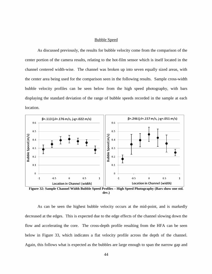
As discussed previously, the results for bubble velocity come from the comparison of the
center portion of the camera results, relating to the hot-film sensor which is itself located in the
channel centered width-wise. The channel was broken up into seven equally sized areas, with
the center area being used for the comparison seen in the following results. Sample cross-width
bubble velocity profiles can be seen below from the high speed photography, with bars
displaying the standard deviation of the range of bubble speeds recorded in the sample at each
location.
Figure 32: Sample Channel Width Bubble Speed Profiles – High Speed Photography (Bars show one std.
dev.)
As can be seen the highest bubble velocity occurs at the mid-point, and is markedly
decreased at the edges. This is expected due to the edge effects of the channel slowing down the
flow and accelerating the core. The cross-depth profile resulting from the HFA can be seen
below in Figure 33, which indicates a flat velocity profile across the depth of the channel.
Again, this follows what is expected as the bubbles are large enough to span the narrow gap and

45
the velocity profile can be considered to be that of a single bubble’s profile, which moves at one
single velocity.
Figure 33: Sample Channel Depth Bubble Speed Profiles - HFA
Again, the best comparison of these two methods is at the mid-points of the profiles. The
exhaustive velocity comparison can be seen in Figure 34 as it varies by volume fraction.
Because the velocity is a function of not only by the volume fraction, but also the superficial
liquid and gas velocities, the near-linear relationship shown for void fraction is not seen. The
velocities reported by the two methods are in close agreement, and as seen in Figure 35, the
difference between the two is less than 10% for volume fractions above .100, and below 30% in
all cases examined. The reason for the increased error for lower void fractions can be attributed
to the fewer interactions with the gas phase, making fluctuations from the liquid phase more
prominent and less likely to be averaged out over even large sample sizes.
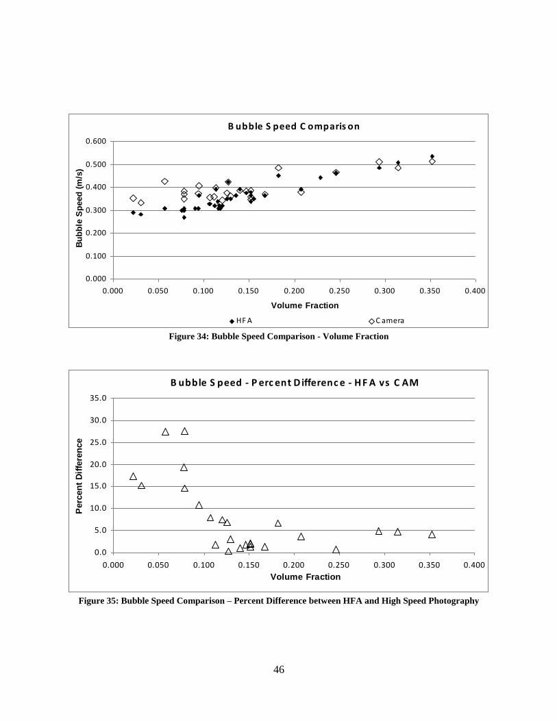
46
B ubble S peed C omparis on
0.000
0.100
0.200
0.300
0.400
0.500
0.600
0.000 0.050 0.100 0.150 0.200 0.250 0.300 0.350 0.400
Volume Fraction
Bu
bb
le S
peed
(m
/s)
HF A C amera
Figure 34: Bubble Speed Comparison - Volume Fraction
B ubble S peed - P erc ent D ifferenc e - H F A vs C AM
0.0
5.0
10.0
15.0
20.0
25.0
30.0
35.0
0.000 0.050 0.100 0.150 0.200 0.250 0.300 0.350 0.400
Volume Fraction
Perc
en
t D
iffe
ren
ce
Figure 35: Bubble Speed Comparison – Percent Difference between HFA and High Speed Photography
47
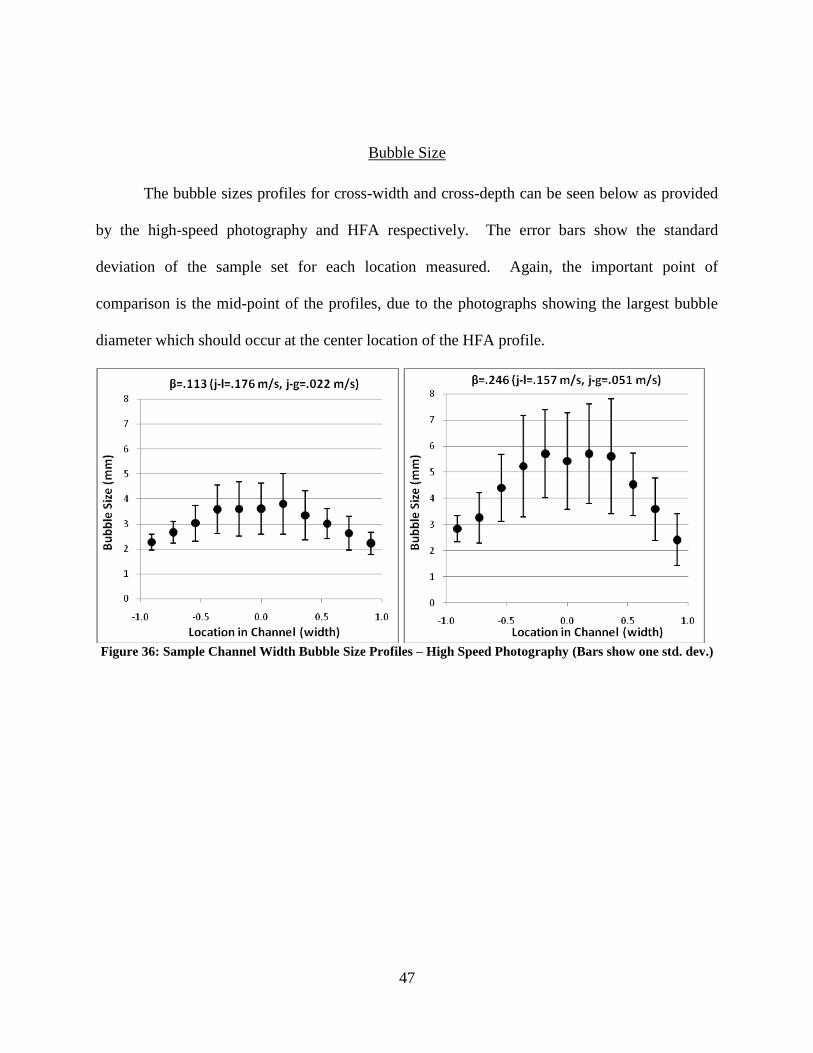
Bubble Size
The bubble sizes profiles for cross-width and cross-depth can be seen below as provided
by the high-speed photography and HFA respectively. The error bars show the standard
deviation of the sample set for each location measured. Again, the important point of
comparison is the mid-point of the profiles, due to the photographs showing the largest bubble
diameter which should occur at the center location of the HFA profile.
Figure 36: Sample Channel Width Bubble Size Profiles – High Speed Photography (Bars show one std. dev.)

48
Figure 37: Sample Channel Depth Bubble Size Profiles – HFA (Bars show one std. dev.)
The slight bias to the far wall for the HFA results that was shown for void fraction once
again is show for the bubble size profile, due to the same deformation effect, with the bubbles
having possibly having artificially higher chord lengths when pinched between the probe and the
wall. The HFA profile does roughly resemble the leading edge of a bubble, as would be
expected if the bubbles are bridging the gap within the narrow channel. Further, the high-speed
camera profiles show maximum at the center of the channel as expected due to the higher rate of
bubble-bubble interaction, encouraging coalescence.The comparison of center average bubble
diameter can be seen below in Figure 38. The results from the high-speed camera are slightly
larger in all cases, but increase with the same rate with volume fraction. The percentage
difference between the two, as seen in Figure 39, has no trend with volume fraction and is evenly
spread out across the data set. The bubble sizes from the imaging seem to be shifted upwards by
a constant factor by around 1.3. Often in the use of hot-film anemometry for larger channels, the
calculated bubble diameter is multiplied by a factor of 1.5 due to the probability of the sensor

49
piercing in between the longest diameter of the bubble (center) or somewhere along the edge.
This statistical analysis is explained in detail by [30] and [31], but refers to a bubble variation in
meeting the sensor in the depth direction where the sensor is the thinnest in direction. Due to the
narrowness of the channel used in this study, this statistical method would not apply because the
bubbles are very nearly the size of the channel or larger, so the probability of striking the longest
diameter of the bubble in the depth direction is extremely high. However, there exists a
probability that a partial hit could occur in the width direction where the sensor is longest and
masked by the needles of the probe. The statistical analysis in this case is unclear because the
geometry of the probe, and the ambiguity of the bubble interaction in the case of a partial hit in
the width direction. Though this could explain an underestimation of the bubble diameter by a
fixed factor on the part of the hot-film analysis.
B ubble S iz e C omparis on
0.00
1.00
2.00
3.00
4.00
5.00
6.00
7.00
8.00
9.00
0.000 0.050 0.100 0.150 0.200 0.250 0.300 0.350 0.400
Volume Fraction
Bu
bb
le S
ize (
mm
)
HF A C amera
Figure 38: Bubble Size Comparison - Volume Fraction

50
B ubble S iz e - P erc ent D ifferenc e - H F A vs C amera
0.0
5.0
10.0
15.0
20.0
25.0
30.0
35.0
40.0
45.0
50.0
0.000 0.050 0.100 0.150 0.200 0.250 0.300 0.350 0.400
Volume Fraction
Perc
en
t D
iffe
ren
ce
Figure 39: Bubble Size Comparison – Percent Difference
Though the results for the velocity show good agreement between the two methods, the
results for the void fraction and bubble size demonstrate the differences that can occur. The
strength of the hot-film is in the quick analysis of large amounts of data, recording nearly 1000
bubble interactions per sampling, though there is an ambiguous nature to each interaction for
which assumptions such as threshold levels must be made. The high-speed video allows the
direct examination of each bubble passage, though the processing is more tedious and is
restricted to the analysis of only a few hundred bubbles. A longer sample time is favorable for
void fraction measurements, which can be limiting for the high-speed photography that requires
large file sizes and slow analysis.

51
CHAPTER FIVE: CONCLUSIONS
The hot-film anemometer is a well established method for use in multi-phase
applications, and highly desired for its simplicity of operation and ability to quickly analyze
large amounts of data. Multiple techniques have been established for the analysis of hot-film
data by various studies, with the most important aspect involving separating the portions of the
signal belonging to each phase. This study employed various techniques in order to demonstrate
the use of the instrument, explore more deeply the methods of phase discrimination, and
ultimately come up with a robust method of analysis favorable for the present geometry.
A vertically oriented acrylic test section with a narrow rectangular channel was connected
to tightly controlled air-water flow loop for the purposes of studying and advancing hot-film
anemometry techniques for multiphase flow. The narrow rectangular channel has applications
for multi-phase heat transfer including miniature high-performance heat exchangers as well as
for steam generation in the power generation industry. The geometry of the channel itself is also
useful for the pairing of multiple measurement instruments, particularly optical devices, for the
purposes of fundamental studies and demonstrations. This fostered ideal conditions for pairing
high-speed video tests with the hot-film data for a large variety of flow conditions.
Through the study and comparison of phase discrimination methods and threshold
selection, it was found that a hybrid technique was ideal for the current situation due to the
hardships of a pure-slope technique in determining bubble diameters. The hybrid technique uses
an amplitude threshold for triggering, and small slope thresholds for finely tuning the edges of
the bubble interactions. This is a method first described by [18], and has since become widely

52
used. The method of amplitude threshold selection came from plotting the void fraction of the
signal for a wide range of threshold values, as suggested by [23], but was taken a step further by
differentiating this curve. It was found that the shape of the derivative consisted of two-peaks
similar to that of the voltage histogram, with an inflection point in the trough between the two
peaks. Though this study showed there were minimal effects in modifying the amplitude
threshold within a range between these peaks, this inflection point was chosen for its easy of
identification and consistency.
With a phase discrimination chosen and a robust method of threshold selection, a wide
range of flow conditions were studied. Volume fractions ranging from 2% to 35% were studied,
spanning across a range of bubbly flows. The void fraction comparisons were difficult due to the
limiting nature of the high-speed video for processing large amounts of data, but the hot-film
followed an expected trend and demonstrated high repeatability. The velocity was found to be in
very close agreement between the HFA and high-speed video, staying within 10% for volume
fractions above 10%, but still remaining under a 30% difference for even as low as the 2%
volume fraction. The trends with volume fraction between the HFA and high-speed results were
very similar, with the high-speed data seeming to be shifted off by a constant factor, but still
remaining within the 30% range.

53
APPENDIX A: LOCATING CHANNEL CENTER

54
To be able to accurately relate the micrometer reading to the location of the probe sensor
within the channel, tests were run to locate the exact center using the known principles of
velocity profiles for fluids. The velocity profile is maximum at the center of the channel, so
employing a pure water flow, the micrometer reading that reports the highest voltage would be
the one that corresponds to the center. The location of the probe within the channel could then
be known from the distance of the micrometer setting from the established reference point.
The first tests taken were a broad sweep across the channel, in order to find the general
location of the peak. The second tests focused more closely on the area of the peak in order to
pinpoint the exact location with a higher resolution. Because of the sensitivity of the probe and
expected flat profile at the center of the channel, the tests were taken quickly to avoid the effects
of any slight drift in temperature or flow rate, both of which were monitored closely. Samples
were taken at 5000Hz for 13 seconds at each location, and the voltage value was taken as the
average for each block of data. Both the temperature and flow rate were found to not fluctuate
by more than 1% during the tests.
The tests were in good agreement with each other, pinpointing the center of the channel
to correspond to the micrometer reading of .14 inches. Sample results can be seen below, one
from the broad sweep, and one for the more focused sweep.

55
Figure 40: Channel Depth Tests Results

56
APPENDIX B: ERROR PROPOGATION AND UNCERTAINTY

57
Uncertainty values for measured quantities including void fraction, bubble speed, and
bubble size as resulting from both HFA and High-Speed video analysis were found via
repeatability tests under multiple conditions using a pooled standard deviation with relative
standard deviation also reported. This is the method applied by [32] and [33], for which similar
conclusions for HFA local void fraction were found as to that shown here. The summary of the
results can be seen in Table 3, with in-depth details found below.
Equation 3: Pool Standard Deviation (k=number of sets, n=number of samples in set)
Table 3: HFA and Camera Uncertainty Analysis
Std Dev %
HFA Local VF 0.00877 10.63
Ave. Diam. (mm) 0.18189 6.40
Ave. Vel. (m/s) 0.01569 4.84
Camera Ave. VF 0.00912 12.77
Local VF 0.02584 21.02
Ave. Diam. (mm) 0.28627 7.72
Ave. Vel. (m/s) 0.01804 4.99
Local Void Fraction - HFA STD DEV N
T-30 T-50
0.06039 0.06478 0.00310 2
T-29 T-33 T-34 T-35 T-36
0.06335 0.0874 0.074 0.07554 0.0807 0.00891 4
T-31 T-43 T-63
0.09943 0.1155 0.116 0.00946 3
T-32 T-37
0.06917 0.08 0.01058 2
Pooled %
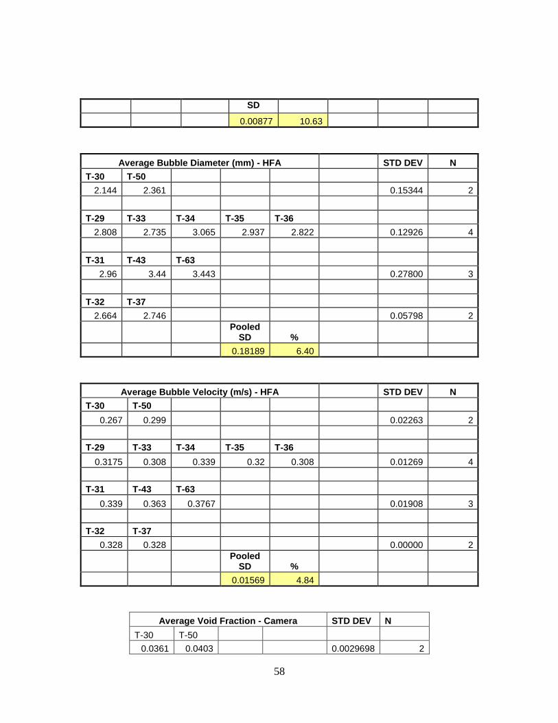
58
SD
0.00877 10.63
Average Bubble Diameter (mm) - HFA STD DEV N
T-30 T-50
2.144 2.361 0.15344 2
T-29 T-33 T-34 T-35 T-36
2.808 2.735 3.065 2.937 2.822 0.12926 4
T-31 T-43 T-63
2.96 3.44 3.443 0.27800 3
T-32 T-37
2.664 2.746 0.05798 2
Pooled
SD %
0.18189 6.40
Average Bubble Velocity (m/s) - HFA STD DEV N
T-30 T-50
0.267 0.299 0.02263 2
T-29 T-33 T-34 T-35 T-36
0.3175 0.308 0.339 0.32 0.308 0.01269 4
T-31 T-43 T-63
0.339 0.363 0.3767 0.01908 3
T-32 T-37
0.328 0.328 0.00000 2
Pooled
SD %
0.01569 4.84
Average Void Fraction - Camera STD DEV N
T-30 T-50
0.0361 0.0403 0.0029698 2
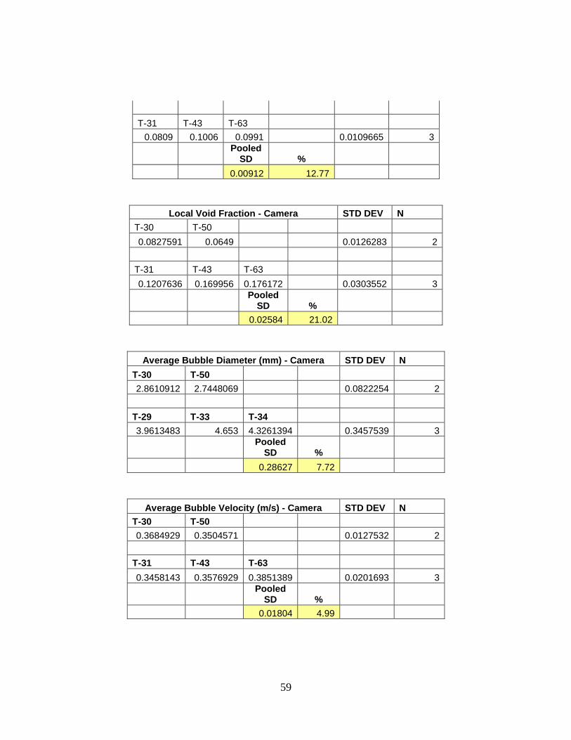
59
T-31 T-43 T-63
0.0809 0.1006 0.0991 0.0109665 3
Pooled
SD %
0.00912 12.77
Local Void Fraction - Camera STD DEV N
T-30 T-50
0.0827591 0.0649 0.0126283 2
T-31 T-43 T-63
0.1207636 0.169956 0.176172 0.0303552 3
Pooled
SD %
0.02584 21.02
Average Bubble Diameter (mm) - Camera STD DEV N
T-30 T-50
2.8610912 2.7448069 0.0822254 2
T-29 T-33 T-34
3.9613483 4.653 4.3261394 0.3457539 3
Pooled
SD %
0.28627 7.72
Average Bubble Velocity (m/s) - Camera STD DEV N
T-30 T-50
0.3684929 0.3504571 0.0127532 2
T-31 T-43 T-63
0.3458143 0.3576929 0.3851389 0.0201693 3
Pooled
SD %
0.01804 4.99

60
APPENDIX C: HFA SIGNAL ANALYSIS CODE
61
Pure Slope Phase Discrimination and Void Fraction Calculation Code
% Input Test Parameters BlockS=131072; %Block Size freq=10000; %Sampling Frequency nBlock=84; %Total Number of Blocks Recorded (whole test) nPoints=11; %Number of Locations Examined in Channel C=7; %Number of Blocks Sampled Per Location in Channel K=C*BlockS; %Total Number of Points in Each Location Sample dthresh=36; %Primary Slope Threshold dthresh2=5; %Secondary Slope Threshold dthresh3=10; %Buffer Slope Value
% Loads Files M=zeros(BlockS,nBlock); for i=1:nBlock if i<10 filename=['AW-TEST-T-42/AW-TEST-T-42.B000',int2str(i)]; elseif i>=10 && i<100 filename=['AW-TEST-T-42/AW-TEST-T-42.B00',int2str(i)]; else filename=['AW-TEST-T-42/AW-TEST-T-42.B0',int2str(i)]; end Tempdata=dlmread(filename); M(:,i)=Tempdata(:,3); end disp('Files Read')
% Builds voltage vectors V=zeros(K,nPoints); for m=1:nPoints z=C*(m-1); V(:,m)=[M(:,1+z);M(:,2+z);M(:,3+z);M(:,4+z);M(:,5+z);M(:,6+z);M(:,7+z)]; end % Builds time vector t=zeros(K,1); for i=1:K t(i)=(i-1)/freq; end % Takes first derivative of voltage data dV=zeros(K,nPoints); for m=1:nPoints; for i=2:K-1 dV(i,m)=(V(i+1,m)-V(i-1,m))/(t(i+1)-t(i-1)); end end disp('Vectors Created')
for m=1:nPoints % Use pure slope (lead and trail) thresh to calculate void fraction dV(1,m)=dthresh3;

62
dV(2,m)=-dthresh3; dV(3,m)=dthresh3; Phase=zeros(K,1); b=0; water=1; air=0; bub=0;
% LEAD PORTION – Look for front interfaces for i=1:K if bub==0 if dV(i,m)<=-dthresh Phase(i)=air; bub=1; else Phase(i)=water; end else if dV(i,m)>=dthresh2 Phase(i)=water; bub=0; else Phase(i)=air; end end end % TRAIL PORTION – Look for rear interfaces for i=1:K if dV(i,m)>=dthresh j=i; while dV(j,m)>=-dthresh2 j=j-1; end while dV(j,m)<=dthresh2 Phase(j)=air; j=j-1; end end end %Track Air Phase for i=1:K if Phase(i)==air b=b+1; end end %Void Fractions VF(m)=b/K; end
Hybrid (Amplitude Trigger) Phase Discrimination and Void Fraction Calculation Code
% Input Test Parameters
BlockS=131072; %Block Size
63
freq=10000; %Sampling Frequency
nBlock=77; %Total Number of Blocks Recorded (whole test)
nPoints=11; %Number of Locations Examined in Channel
C=7; %Number of Blocks Sampled Per Location in Channel
K=C*BlockS; %Total Number of Points in Each Location Sample
dthresh=36; %Primary Slope Threshold
dthresh2=5; %Secondary Slope Threshold
dthresh3=10; %Buffer Slope Value
% Loads Files
M1=zeros(BlockS,nBlock);
for i=1:nBlock
if i<10
filename=['AW-TEST-T-65/AW-TEST-T-65.B000',int2str(i)];
elseif i>=10 && i<100
filename=['AW-TEST-T-65/AW-TEST-T-65.B00',int2str(i)];
else
filename=['AW-TEST-T-65/AW-TEST-T-65.B0',int2str(i)];
end
Tempdata = dlmread(filename);
M(:,i)=Tempdata(:,3);
end
clear Tempdata
disp('Files Read')
%Builds voltage vectors
V=zeros(K,nPoints);
for m=1:nPoints
z=C*(m-1);
V(:,m)=[M(:,1+z);M(:,2+z);M(:,3+z);M(:,4+z);M(:,5+z);M(:,6+z);M(:,7+z)];
end
clear M*
%Builds time vector
t=zeros(K,1);
for i=1:K
t(i)=(i-1)/freq;
end
%Takes first derivative of voltage data
dV=zeros(K,nPoints);
for m=1:nPoints;
for i=2:K-1
dV(i,m)=(V(i+1,m)-V(i-1,m))/(t(i+1)-t(i-1));
end
end
disp('Vectors Created')
for m=1:nPoints
%Use hybrid technique to calculate void fraction
Phase=zeros(K,1);
water=1;
air=0;
n=400;
thresh=zeros(n+1,1);
VF=zeros(n+1,1);
64
for s=1:n+1
a=0;
thresh(s)=max(V(:,m))-(1/n)*(s-1)*(max(V(:,m))-min(V(:,m)));
for i=2:K
Phase(i)=water;
if V(i,m)<thresh(s) && V(i-1,m)>thresh(s)
j=i;
while dV(j,m)<-dthresh2
Phase(j)=air;
j=j-1;
end
elseif V(i,m)<thresh(s)
Phase(i)=air;
elseif V(i,m)>thresh(s) && V(i-1,m)<thresh(s)
j=i;
while dV(j,m)>dthresh2
Phase(j)=water;
j=j-1;
end
end
end
for i=1:K
if Phase(i)==air
a=a+1;
end
end
VF(s)=a/K;
end
VF
end
Bubble Velocity Cross Correlation Code
% Input Test Parameters
BlockS=131072; %Block Size
freq=10000; %Sampling Frequency
nBlock=77; %Total Number of Blocks Recorded (whole test)
nPoints=11; %Number of Locations Examined in Channel
C=7; %Number of Blocks Sampled Per Location in Channel
K=C*BlockS; %Total Number of Points in Each Location Sample
dthresh=36; %Primary Slope Threshold
dthresh2=5; %Secondary Slope Threshold
dthresh3=10; %Buffer Slope Value
% Loads Files M1=zeros(BlockS,nBlock); M2=zeros(BlockS,nBlock); for i=1:nBlock if i<10 filename=['AW-TEST-T-65/AW-TEST-T-65.B000',int2str(i)]; elseif i>=10 && i<100 filename=['AW-TEST-T-65/AW-TEST-T-65.B00',int2str(i)]; else

65
filename=['AW-TEST-T-65/AW-TEST-T-65.B0',int2str(i)]; end Tempdata = dlmread(filename); M1(:,i)=Tempdata(:,3); M2(:,i)=Tempdata(:,2); end clear Tempdata disp('Files Read')
% Builds voltage vectors V=zeros(K,nPoints); Vb=zeros(K,nPoints); for m=1:nPoints
z=C*(m-1);
V(:,m)=[M1(:,1+z);M1(:,2+z);M1(:,3+z);M1(:,4+z);M1(:,5+z);M1(:,6+z);
M1(:,7+z)];
Vb(:,m)=[M2(:,1+z);M2(:,2+z);M2(:,3+z);M2(:,4+z);M2(:,5+z);M2(:,6+z);
M2(:,7+z)]; end clear M* % Builds time vector t=zeros(K,1); for i=1:K t(i)=(i-1)/freq; end % Takes first derivative of voltage data dV=zeros(K,nPoints); dVb=zeros(K,nPoints); for m=1:nPoints; for i=2:K-1 dV(i,m)=(V(i+1,m)-V(i-1,m))/(t(i+1)-t(i-1)); dVb(i,m)=(Vb(i+1,m)-Vb(i-1,m))/(t(i+1)-t(i-1)); end end disp('Vectors Created')
for m=1:nPoints water=1; air=0; n=40; for s=1:n+1 %Phase discrimination (hybrid) first sensor
Phase=zeros(K,1);
if s<=n/2 %Thresh limits from void fraction code
thresh(s)=1.271+(4/n)*(s-1)*(1.379-1.271);
else
thresh(s)=1.379;
end
a=0; for i=2:K Phase(i)=water; if V(i,m)<thresh(s) && V(i-1,m)>thresh(s) j=i;
66
while dV(j,m)<-dthresh2 Phase(j)=air; j=j-1; end elseif V(i,m)<thresh(s) Phase(i)=air; elseif V(i,m)>thresh(s) && V(i-1,m)<thresh(s) j=i; while dV(j,m)>dthresh2 Phase(j)=water; j=j-1; end end end for i=1:K if Phase(i)==air a=a+1; end end VF(s)=a/K;
%Phase discrimination (hybrid) second sensor Phaseb=zeros(K,1); if s>=n/2+1 %Thresh limits from void fraction code threshb(s)=2.215+(4/n)*((s-n/2)-1)*(2.611-2.215); else threshb(s)=2.611; end b=0; for i=2:K Phaseb(i)=water; if Vb(i,m)<threshb(s) && Vb(i-1,m)>threshb(s) j=i; while dVb(j,m)<-dthresh2 Phaseb(j)=air; j=j-1; end elseif Vb(i,m)<threshb(s) Phaseb(i)=air; elseif Vb(i,m)>threshb(s) && Vb(i-1,m)<threshb(s j=i; while dVb(j,m)>dthresh2 Phaseb(j)=water; j=j-1; end end end for i=1:K if Phaseb(i)==air b=b+1; end end VFb(s)=b/K;

67
%Cross Correlation K1=length(Phase); range=200; Prod=zeros(K1-2*range,1); R=zeros(2*range+1,1); tau=zeros(2*range+1,1); for i=-range:range for j=range+1:K1-range Prod(j)=(Phase(j))*(Phaseb(j+i))*.0001; end R(i+range+1)=sum(Prod)/t(K1); tau(i+range+1)=i*.0001; end [C,I]=max(R); tau2(s,m)=tau(I) end
figure,plot3(thresh,threshb,tau2(:,m)) end
Chord Length Distribution and Average Diameter Code
% Input Test Parameters BlockS=131072; %Block Size freq=10000; %Sampling Frequency nBlock=77; %Total Number of Blocks Recorded (whole test) nPoints=11; %Number of Locations Examined in Channel C=7; %Number of Blocks Sampled Per Location in Channel
K=C*BlockS; %Total Number of Points in Each Location Sample
dthresh=36; %Primary Slope Threshold
dthresh2=5; %Secondary Slope Threshold
dthresh3=10; %Buffer Slope Value
% Loads Files M1=zeros(BlockS,nBlock); for i=1:nBlock if i<10 filename=['AW-TEST-T-65/AW-TEST-T-65.B000',int2str(i)]; elseif i>=10 && i<100 filename=['AW-TEST-T-65/AW-TEST-T-65.B00',int2str(i)]; else filename=['AW-TEST-T-65/AW-TEST-T-65.B0',int2str(i)]; end Tempdata = dlmread(filename); M(:,i)=Tempdata(:,3); end clear Tempdata disp('Files Read')
% Builds voltage vectors

68
V=zeros(K,nPoints); for m=1:nPoints z=C*(m-1); V(:,m)=[M(:,1+z);M(:,2+z);M(:,3+z);M(:,4+z);M(:,5+z);M(:,6+z);M(:,7+z)]; end clear M* % Builds time vector t=zeros(K,1); for i=1:K t(i)=(i-1)/freq; end % Takes first derivative of voltage data dV=zeros(K,nPoints); for m=1:nPoints; for i=2:K-1 dV(i,m)=(V(i+1,m)-V(i-1,m))/(t(i+1)-t(i-1)); end end disp('Vectors Created')
for m=1:nPoints n=400; thresh=zeros(n+1,nPoints); VF=zeros(n+1,nPoints); for s=1:n+1 thresh(s,m)=max(V(:,m))-(1/n)*(s-1)*(max(V(:,m))-min(V(:,m))); end %Use hybrid technique to calculate void fraction
water=1;
air=0;
ST=size(thresh);
Phase=zeros(K,1);
Chord=zeros(100,ST(1));
for s=1:ST(1)
a=0;
for i=2:K
Phase(i)=water;
if V(i,m)<thresh(s,m) && V(i-1,m)>thresh(s,m)
j=i;
while dV(j,m)<-dthresh2
Phase(j)=air;
j=j-1;
end
elseif V(i,m)<thresh(s,m)
Phase(i)=air;
elseif V(i,m)>thresh(s,m) && V(i-1,m)<thresh(s,m)
j=i;
while dV(j,m)>dthresh2
Phase(j)=water;
j=j-1;
end
end
end
69
for i=1:K
if Phase(i)==air
a=a+1;
end
end
VF(s,m)=a/K;
%Extracts Chord Length
L=0;
j=1;
for i=2:K
if Phase(i)==air
L=L+1;
Chord(j,s)=L+1;
else
L=0;
end
if Phase(i)==water && Phase(i-1)==air
ChordLoc(j,s)=t(i-1);
j=j+1;
end
end
end
BL=zeros(m,ST(1));
%Calculates bubble size and speed
delta=1.016; %Distance between sensors (mm)
Vel=delta/tau(m); %Interfacial bubble velocity (mm/s)
Bub=.0001*Chord*Vel;
for s=1:ST(1)
edges=0:1:max(Chord(:,s));
edges(1)=.001;
hista=histc(Chord(:,s),edges);
[A,IX]=sort(hista,'descend');
sum=0;
freq=0;
for i=1:max(edges)
freq=hista(i)*edges(i)+freq;
sum=hista(i)+sum;
end
freq;
sum;
rt=.0001*freq/sum; %average bubble residence time (s)
BL(s,m)=rt*Vel; %average bubble length (mm)
end
end

70
LIST OF REFERENCES
[1] R. Kumar, C. C. Maneri, and T. D. Strayer, "Modeling and Numerical Prediction of Flow
Boiling in a Thin Geometry," Journal of Heat Transfer, vol. 126, p. 22, 2004.
[2] R. Kumar, T. A. Trabold, and C. C. Maneri, "Experiments and Modeling in Bubbly
Flows at Elevated Pressures," Journal of Fluids Engineering, vol. 125, pp. 469-478,
2003.
[3] R. Kumar, M. Gottmann, and K. R. Sridhar, "Film thickness and wave velocity
measurements in a vertical duct," Journal of Fluids Engineering, vol. 124, p. 634, 2002.
[4] R. Kumar and T. A. Trabold, "High Pressure Annular Two Phase Flow in a Narrow Duct:
Part II--Three Field Modeling," Journal of Fluids Engineering, vol. 122, pp. 375-383,
2000.
[5] R. Kumar and T. A. Trabold, "Effect of Pressure With Wall Heating in Annular Two-
Phase Flow," Journal of Fluids Engineering, vol. 125, p. 84, 2003.
[6] T. Wilmarth and M. Ishii, "Two-phase flow regimes in narrow rectangular vertical and
horizontal channels," International Journal of Heat and Mass Transfer, vol. 37, pp. 1749-
1758, 1994.
[7] P. F. Vassallo and R. Kumar, "Liquid and gas velocity measurements using LDV in air-
water duct flow," Experimental Thermal and Fluid Science, vol. 19, pp. 85-92, 1999.
[8] G. J. Kirouac, T. A. Trabold, P. F. Vassallo, W. E. Moore, and R. Kumar,
"Instrumentation development in two-phase flow," Experimental Thermal and Fluid
Science, vol. 20, pp. 79-93, 1999.
[9] G. Comte-Bellot and J. F. Foss, "Thermal Anemometry," in Springer Handbook of
Experimental Fluid Mechanics, C. Tropea, A. L. Yarin, and J. F. Foss, Eds. New York:
Springer-Verlag, 2007, pp. 229-287.
[10] "IFA 300 Constant Temperature Anemometer System Operation Manual," Revision C ed
Shoreview, MN: TSI Inc., 2007.
[11] R. H. S. Winterton and J. S. Munaweera, "Bubble size in two-phase gas-liquid bubbly
flow in ducts," Chemical Engineering and Processing, vol. 40, pp. 437-447, 2001.
71
[12] K. Mishima, T. Hibikia, and H. Nishiharaa, "Some Characteristics of Gas-Liquid Flow in
Narrow Rectangular Ducts," International Journal of Multiphase Flow, vol. 19, pp. 115-
124, 1993.
[13] O. C. Jones, Jr. and N. Zuber, "Slug-annular transition with particular reference to narrow
rectangular ducts.," in Two-Phse Momentum, Heat and Mass Transfer in Chemical,
Process and Energy Engineering Systems. vol. 1, F. Durst, G. V. Tsiklauri, and N. H.
Afgan, Eds. Washington DC: Hemisphere, 1979, pp. 345-355.
[14] M. Ishii, "One-Dimensional Drift Flux Model and Constitutive Equations for Relative
Motion Between Phases in Various Two-Phase Flow Regimes," in ANL Report. vol.
ANL-77-47, 1977.
[15] J. L. Xu, P. Cheng, and T. S. Zhao, "Gas-liquid two-phase flow regimes in rectangular
channels with mini/micro gaps," International Journal of Multiphase Flow, vol. 25, pp.
411-432, 1999.
[16] T. Hibiki and K. Mishima, "Flow regime transition criteria for upward two-phase flow in
vertical narrow rectangular channels," Nuclear Engineering and Design, vol. 203, pp.
117-131, 2001.
[17] K. Bremhorst and D. B. Gilmore, "Response of Hot Wire Anemometer Probes to A
Stream of Air Bubbles in a Water Flow," Journal of Physics E: Scientific Instruments,
vol. 9, pp. 347-352, 1976.
[18] B. Farrar, A. L. Samways, J. Ali, and H. H. Bruun, "A Computer-Based Hot-Film
Technique for Two-Phase Flow Measurements," Measurement Science and Technology,
vol. 6, pp. 1528-1537, 1995.
[19] B. Farrar and H. H. Bruun, "Interaction Effects Between a Cylindrical Hot-Film
Anemometer Probe and Bubbles in Air/Water and Oil/Water Flows," Journal of Physics
E: Scientific Instruments, vol. 22, p. 114, 1989.
[20] J. Rensen, S. Luther, J. de Vries, and D. Lohse, "Hot-Film Anemometry in Bubbly Flow
I: Bubble-Probe Interaction," International Journal of Multiphase Flow, vol. 31, pp. 285-
301, 2005.
[21] H. Toral, "A Study of the Hot Wire Anemometer for Measuring Void Fraction in Two
Phase Flow," Journal of Physics E: Scientific Instruments, vol. 14, pp. 882-827, 1981.
[22] T. A. Trabold, W. E. Moore, and W. O. Morris, "Hot-Film Anemometer Measurements
in Adiabatic Two-Phase Refrigerant Flow through a Vertical Duct," in ASME Fluids
Engineering Division Summer Meeting, Vancouver, B.C., 1997.

72
[23] F. Resch, H. Leutheusser, and S. Alemu, "Bubbly Two-Phase Flow in Hydraulic Jump,"
Journal of the Hydraulics Division, vol. 100, pp. 137-149, 1974.
[24] T. A. Trabold and R. Kumar, "High Pressure Annular Two Phase Flow in a Narrow Duct:
Part I--Local Measurements in the Droplet Field," Journal of Fluids Engineering, vol.
122, pp. 364-374, 2000.
[25] N. T. Thang and M. R. Davis, "The Structure of Bubbly Flow through Venturis,"
International Journal of Multiphase Flow, vol. 5, pp. 17-37, 1979.
[26] R. van der Welle, "Void Fraction, Bubble Velocity and Bubble Size in Two-Phase Flow,"
International Journal of Multiphase Flow, vol. 11, pp. 317-345, 1985/6// 1985.
[27] G. Wang and C. Y. Ching, "Measurement of Multiple Gas-Bubble Velocities in Gas–
Liquid Flows Using Hot-Film Anemometry," Experiments in Fluids, vol. 31, pp. 428-
439, 2001.
[28] P. F. Vassallo, T. A. Trabold, R. Kumar, and D. M. Considine, "Slug-to-annular regime
transitions in R-134a flowing through a vertical duct," International Journal of
Multiphase Flow, vol. 27, pp. 119-145, 2001.
[29] J. Canny, "A Computational Approach to Edge Detection," IEEE Transactions on
Pattern Analysis and Machine Intelligence, vol. 8, pp. 679-698, 1986.
[30] W. Liu and N. N. Clark, "Relationships between distributions of chord lengths and
distributions of bubble sizes including their statistical parameters," International Journal
of Multiphase Flow, vol. 21, pp. 1073-1089, 1995.
[31] W. Liu, N. N. Clark, and A. I. Karamavruc, "Relationships between bubble size
distributions and chord-length distribution in heterogeneously bubbling systems,"
Chemical Engineering Science, vol. 53, pp. 1267-1276, 1998.
[32] T. A. Trabold and R. Kumar, "Vapor core turbulence in annular two-phase flow,"
Experiments in Fluids, vol. 28, pp. 187-194, 2000.
[33] T. A. Trabold, R. Kumar, and P. F. Vassallo, "Experimental study of dispersed droplets
in high-pressure annular flows," Journal of Heat Transfer, vol. 121, pp. 924-933, 1999.
Recommended