1
http://mipav.cit.nih.gov
MEDICAL IMAGE PROCESSING AND
REGISTRATION
IN MIPAV
2
Evan McCreedy
email: [email protected]
(301) 496-3323
Biomedical Image Processing Research Services Section
(BIRSS)
http://mipav.cit.nih.gov
MIPAV TEAM
3
Employees
Ruida Cheng
William Gandler
Matthew McAuliffe
Evan McCreedy
Contractors
Alexandra Bokinsky, Geometric Tools Inc. (Visualization)
Olga Vovk, SRA International Inc. (Technical Writing)
Alumni
Paul Hemler, Agatha Munzon, Nishith Pandya,
Justin Senseney, Sara Shen, Beth Tyriee, Hailong Wang

4
– Filters
– Gaussian blurring, Laplacian, curvature, other higher order derivatives, median, gradient magnitude, edge detection, etc.
– Anisotropic diffusion
– Frequency domain (FFT, etc)
– Registration
• Landmark – least squares, Thin-plate spline
• AFNI registration technique
• General Linear Registration (multiple cost function including, normalized and standard mutual information, correlation, least-squares, etc) and user selectable degree of freedom (DOF, 12 – affine, 6 – rigid,)
– Image transformations or resampling
– nearest neighbor, tri-linear, sinc, bSpline and others interpolation methods.
– Skull stripping (BSE, BET)
– Midsagittal line alignment
– Histogram equalization and matching
– Shading correction
– Microscopy
– FRET, FRAP, Co-localization
MIPAV ALGORITHMS

5
MIPAV ALGORITHMS (CONT.)
– Morphological operators (2D and 3D)
• erode, dilate, open, close, distance, etc.
– Segmentation
– Fuzzy C-means
– Level set
– Thresholding
– Watershed
– Reslice 3D dataset to isotropic voxels
– linear, cubic, cubic bspline.
– Surface extraction
– And more...

IMAGE PROCESSING DIMENSIONALITY
6
• 2D - image plane (slice)
• 2.5D - (3D treated as set of slices)
• 3D - (3D processed as volume)
• 3.5D
• 4D

7

FILTERS
8

9
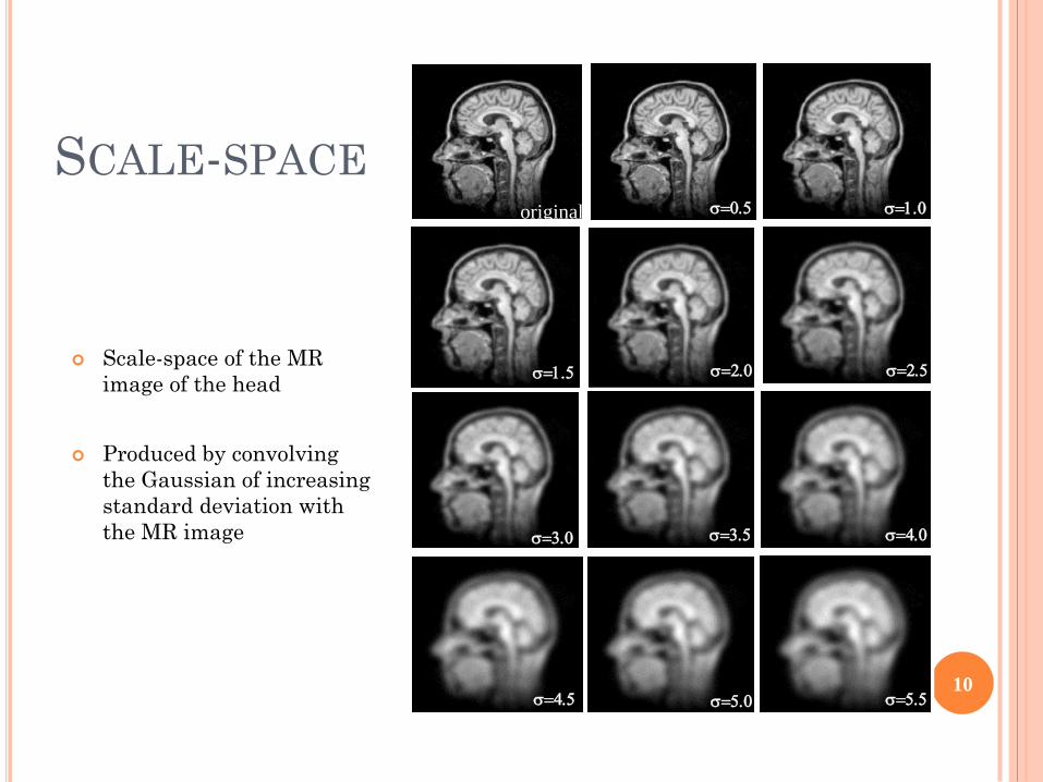
SCALE-SPACE
Scale-space of the MR
image of the head
Produced by convolving
the Gaussian of increasing
standard deviation with
the MR image
10
s=1.0
s=3.0
s=5.0
original s=0.5
s=1.5 s=2.0 s=2.5
s=3.5 s=4.0
s=4.5 s=5.5

GRADIENT MAGNITUDE
1D EXAMPLE
11
Original signal
First derivative
Gradient magnitude

IMPORTANCE OF SCALE
12
Binary Object -
square formed from disks
( b )
Gradient Magnitude
s = 10.0
( a )
Gradient Magnitude s = 1.0
( c )
IGM(x,y) = (Ix2 + Iy
2)0.5 - gradient
magnitude

IMPORTANCE OF SCALE
(GRADIENT MAGNITUDE OF CT IMAGE)
13
Axial CT image Gradient magnitude
(sigma = 1.0)
Gradient magnitude
(sigma = 4.0)

LAPLACIAN
14
Original signal
First derivative
Second derivative
yyxx III =2

LAPLACIAN
15
Original MR Image Laplacian of MR Image Zero crossings

MEDIAN FILTERING
16
Image with noise Median filter image Gaussian smoothed image

MEDIAN FILTERING
17
5 Iterations 1 Iteration Original MR Image
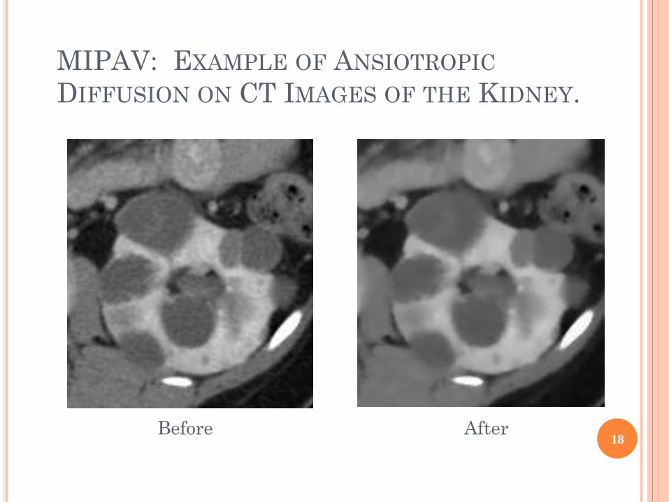
MIPAV: EXAMPLE OF ANSIOTROPIC
DIFFUSION ON CT IMAGES OF THE KIDNEY.
18 Before After

FOURIER TRANSFORM EXAMPLES
19
FFT xf Image
Multiplication IFFT
Filtered
Image
Filter (high-pass)

20
SHADING CORRECTION

REGISTRATION
33

REGISTRATION
34
• Two main classes of problems
– Intra-modality
• Intra - patient
• Inter - patient
– Inter-modality
• Intra - patient
• Inter - patient
• Two main methods
– Extrinsic - landmark methods using surfaces, lines, points.
• Can be automatic or manual identification of landmarks.
– Intrinsic – image intensity base using voxel similarity
measures (i.e. Cross correlation, mutual information, etc.)

REGISTRATION
35
• Transformation matrix establishes geometrical correspondence
between coordinate systems of different images. It is used to
transform one image into the space of the other.
• Many different types but generally in biomedical imaging only a
few classes are use:
– Rigid body
– Global rescale
– Affine
– Non-linear

REGISTRATION
36
• Rigid-body transformations include translations and
rotations. Preserve all lengths and angles.
– 2D -> 3 Degrees of Freedom (DOF)
– 3D -> 6 DOF ( 3 translation and 3 rotation)

REGISTRATION
37
• Global rescale transformations include translations,
rotations, and a single scale parameter. Preserve all
angles and relative lengths.
– 2D -> 4 DOF ( 2 translation + 1 rotation + 1 scale)
– 3D -> 7 DOF ( 3 translation + 3 rotation + 1 scale)
REGISTRATION
38
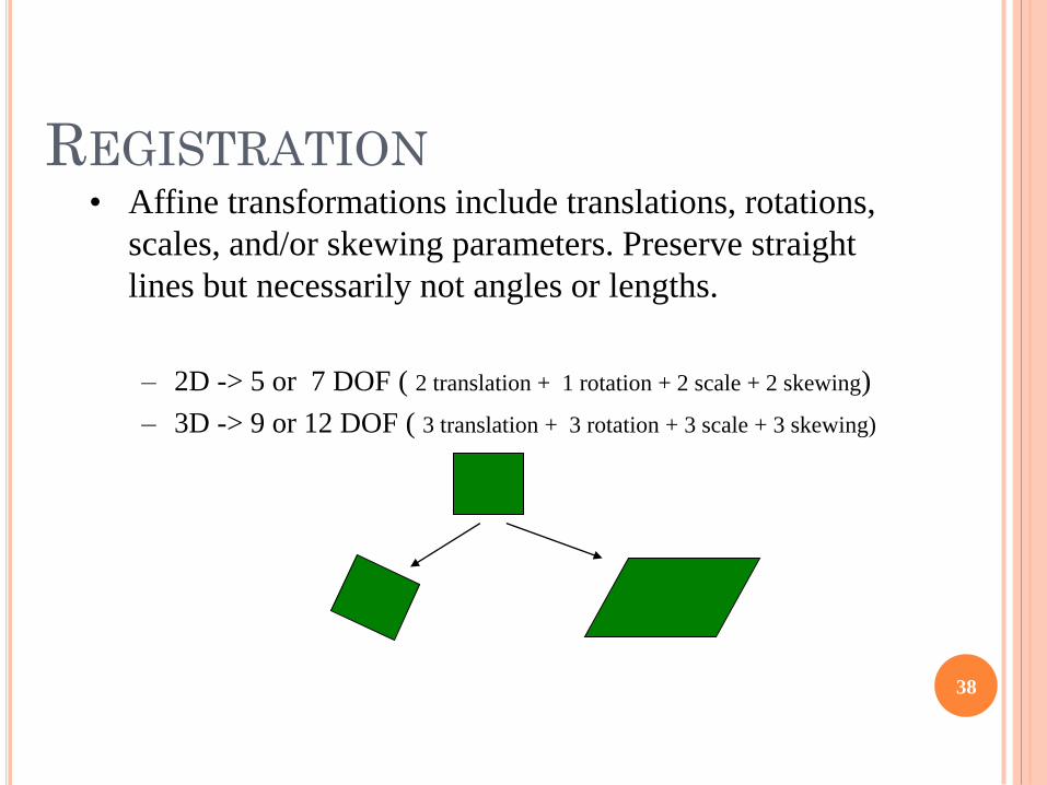
• Affine transformations include translations, rotations,
scales, and/or skewing parameters. Preserve straight
lines but necessarily not angles or lengths.
– 2D -> 5 or 7 DOF ( 2 translation + 1 rotation + 2 scale + 2 skewing)
– 3D -> 9 or 12 DOF ( 3 translation + 3 rotation + 3 scale + 3 skewing)

REGISTRATION
39
• Non-linear transformations are local deformations and
therefore they are the most general.
– 2D -> many DOF
– 3D -> many DOF

INTERPOLATION OPTIONS
Trilinear
Cubic Lagrangian
Quintic Lagrangian
Heptic Lagrangian
Windowed Sinc
Bspline 3rd Order
Bspline 4th Order
40
Increasing complexity
Increasing Process Time
KEY

REGISTRATION
41
4th Order Bspline interpolation Nearest neighbor interpolation

INTERPOLATION DIFFERENCES
42
Trilinear Windowed Sinc Cubic Lagrangian
Contrast increasing

REGISTRATION
43
• Extrinsic Landmark based methods
– can require user interaction
• Manual identification – user intensive
• Automatic identification can be problematic but depends on task
and modality
– can be shown to be less reliable and accurate than intensity
based methods. Depends on modality and task.
– once landmarks are identified registration is very fast.

REGISTRATION
44
• Intrinsic – image intensity at voxels
– “Best” registration is identified by the minimum of some
“cost” function.
– The cost function is an assessment of how good the alignment
between the objects to be registered.
• A high cost should equate to a poor alignment
• A low cost should equate to a good alignment
– Goal
• Find the transformation (matrix) which minimizes the cost
function.

REGISTRATION
45
• Cost functions
– Intra-modality with consistent mapping of intensity values
• Least squares
– Inter-modality or Intra-modality where mapping of intensity
values might vary.
• Normalized correlation
• Correlation ratio
• Normalized mutual information

REGISTRATION
46
• Normalized Mutual Information (NMI) – is base on the entropy of the images
(histogram) and the relationship between voxels – joint entropy.
NMI = ( H(x) + H(y) ) / H(x,y) H( ) = entropy
= - ∑ pi log pi
where p = (histogram count in bin) / total count
• Entropy is a measure of the disorder or unavailability of energy within a
closed system.
• Entropy will have a maximum value if all values of the histogram have equal
probability of occurring (flat histogram) and a minimum when all except one
value has a probability of zero.
– For example, blurring an image reduces noise and thus sharpens the images
histogram, resulting in reduced entropy.

47 Grid with landmarks points
Least squares
registration
(rotation & translation:
rigid)
Thin plate splines registration
(rotation, translation and
scale: non-linear)
LANDMARK REGISTRATION TECHNIQUES
REGISTRATION
48
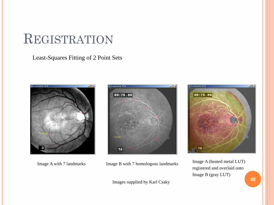
Least-Squares Fitting of 2 Point Sets
Image B with 7 homologous landmarks Image A with 7 landmarks Image A (heated metal LUT)
registered and overlaid onto
Image B (gray LUT)
Images supplied by Karl Csaky
REGISTRATION
49
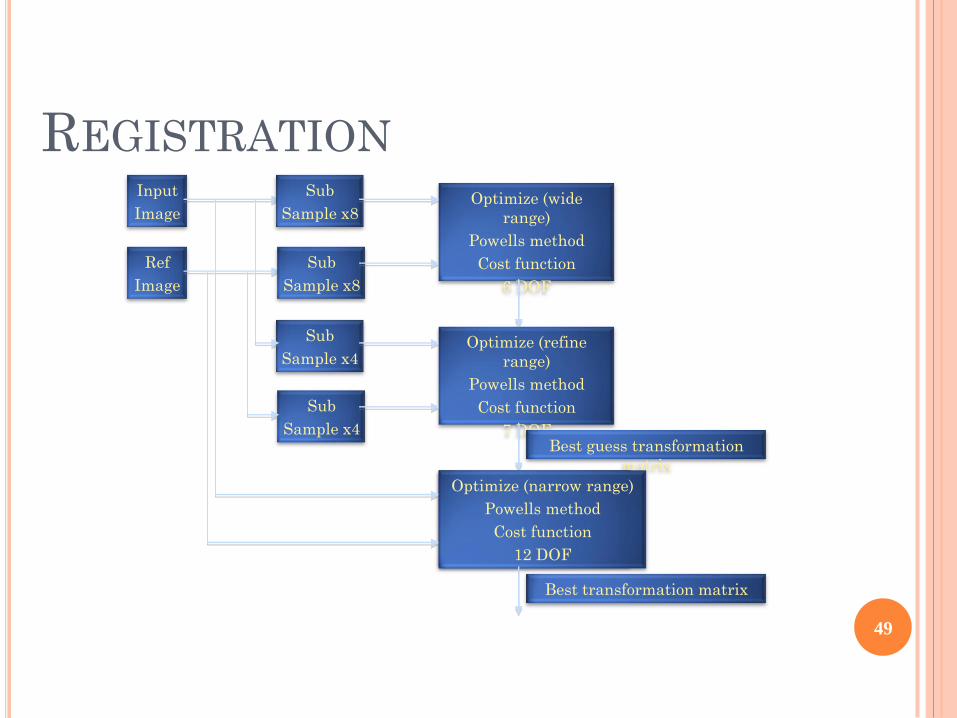
Input
Image
Ref
Image
Sub
Sample x4
Sub
Sample x4
Optimize (refine
range)
Powells method
Cost function
7 DOF
Sub
Sample x8
Sub
Sample x8
Optimize (wide
range)
Powells method
Cost function
6 DOF
Best guess transformation
matrix
Optimize (narrow range)
Powells method
Cost function
12 DOF
Best transformation matrix

SKULL STRIPPING - BET
50
Input
Image
Histogram-based
threshold
estimation
Estimate ellipsoid
used to initialize
surface evolution
Evolve
surface
Based on: Brain Extraction Tool (BET)

51
MIPAV UTILITIES
– Image conversion
– Gray <==> RGB
– 4D <==> 3D
– Between data types
– Image cloning
– Rotation / flipping
– Cropping
– Mask-based quantification
– Intensity projection generation
– Slice extraction / manipulation
– Intensity replacement
– Invert intensity
– Add padding
– Correct spacing
– Image math (operations performed on one image – abs. value, addition, log, etc.)
– Image calculator (operations performed using two source images – difference, multiplication, average, etc.)

THANK YOU!
52
Recommended