Mendelian Randomization
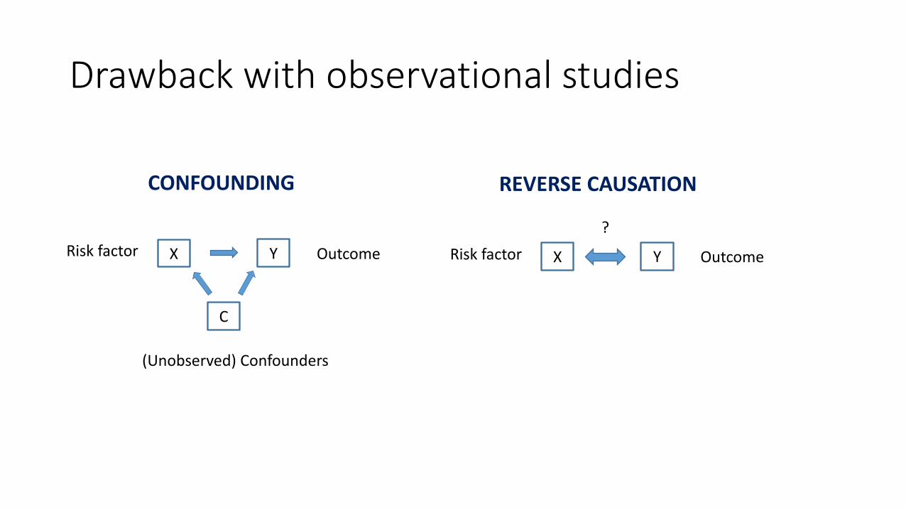
Drawback with observational studies
X Y
C
Risk factor Outcome
(Unobserved) Confounders
X YRisk factor Outcome
?
CONFOUNDING REVERSE CAUSATION
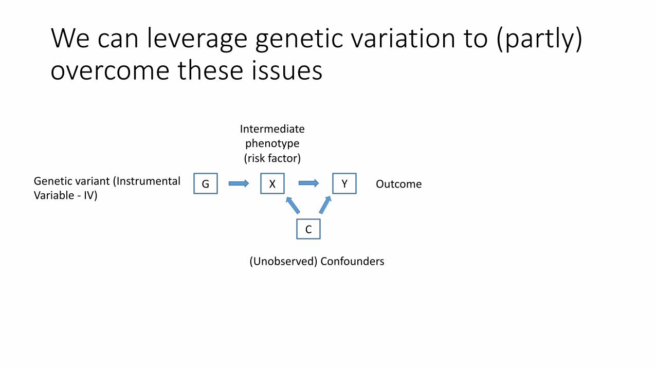
We can leverage genetic variation to (partly) overcome these issues
X Y
C
GGenetic variant (Instrumental Variable - IV)
Intermediate phenotype (risk factor)
Outcome
(Unobserved) Confounders
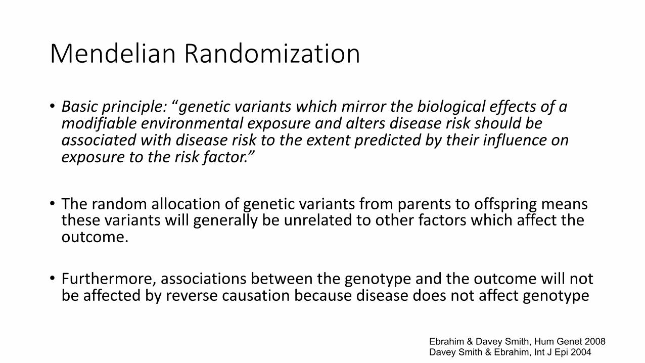
Mendelian Randomization
• Basic principle: “genetic variants which mirror the biological effects of a modifiable environmental exposure and alters disease risk should be associated with disease risk to the extent predicted by their influence on exposure to the risk factor.”
• The random allocation of genetic variants from parents to offspring means these variants will generally be unrelated to other factors which affect the outcome.
• Furthermore, associations between the genotype and the outcome will not be affected by reverse causation because disease does not affect genotype
Ebrahim & Davey Smith, Hum Genet 2008Davey Smith & Ebrahim, Int J Epi 2004
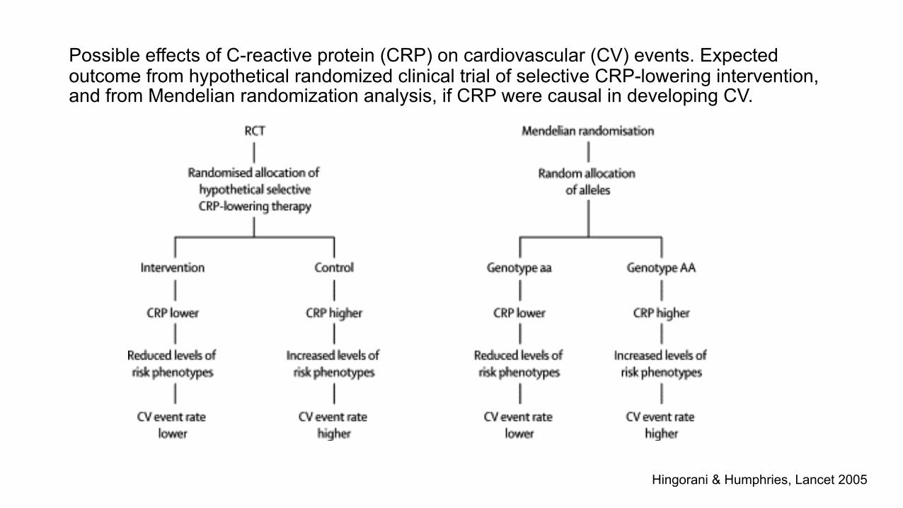
Hingorani & Humphries, Lancet 2005
Possible effects of C-reactive protein (CRP) on cardiovascular (CV) events. Expected outcome from hypothetical randomized clinical trial of selective CRP-lowering intervention, and from Mendelian randomization analysis, if CRP were causal in developing CV.

Three key assumptions in MR analysis
1. G (SNP or a combination of multiple SNPs) is robustly associated with X (risk factor)
2. G is unrelated to any confounders C, that can bias the relationship between G and Y (outcome). In other words, there are no common causes of G and Y (e.g. population stratification)
3. G is related to Y only through its association with X (i.e. no pleiotropy)
X Y
C
G
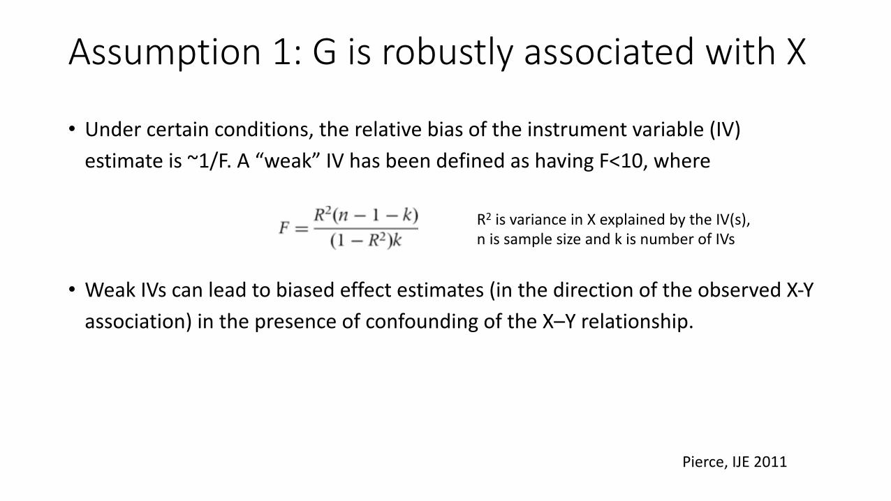
Assumption 1: G is robustly associated with X
• Under certain conditions, the relative bias of the instrument variable (IV) estimate is ~1/F. A “weak” IV has been defined as having F<10, where
• Weak IVs can lead to biased effect estimates (in the direction of the observed X-Y association) in the presence of confounding of the X–Y relationship.
R2 is variance in X explained by the IV(s), n is sample size and k is number of IVs
Pierce, IJE 2011
Assumption 2: No confounding
• G is independent of factors (measured and unmeasured) that confound the X-Y relation
• Since G is randomized at birth and thus is independent of non-genetic confounders and is not modified by the course of disease, the one main concern here is population stratification – i.e. if ancestry is related both to G and Y.
• If you have individual-level data, you can test for this (e.g. PCs)
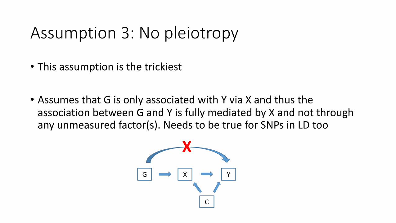
Assumption 3: No pleiotropy
• This assumption is the trickiest
• Assumes that G is only associated with Y via X and thus the association between G and Y is fully mediated by X and not through any unmeasured factor(s). Needs to be true for SNPs in LD too
X Y
C
G
X
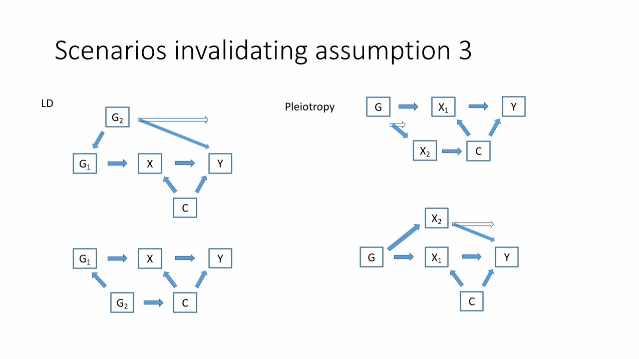
Scenarios invalidating assumption 3
X1 Y
C
G
X Y
C
G1
G2
LD
X Y
C
G1
G2
X1 Y
C
G
Pleiotropy
X2
X2
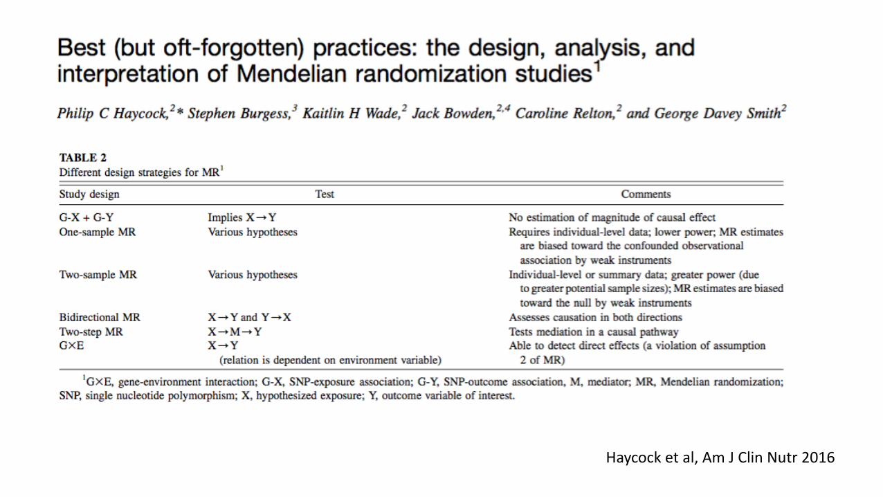
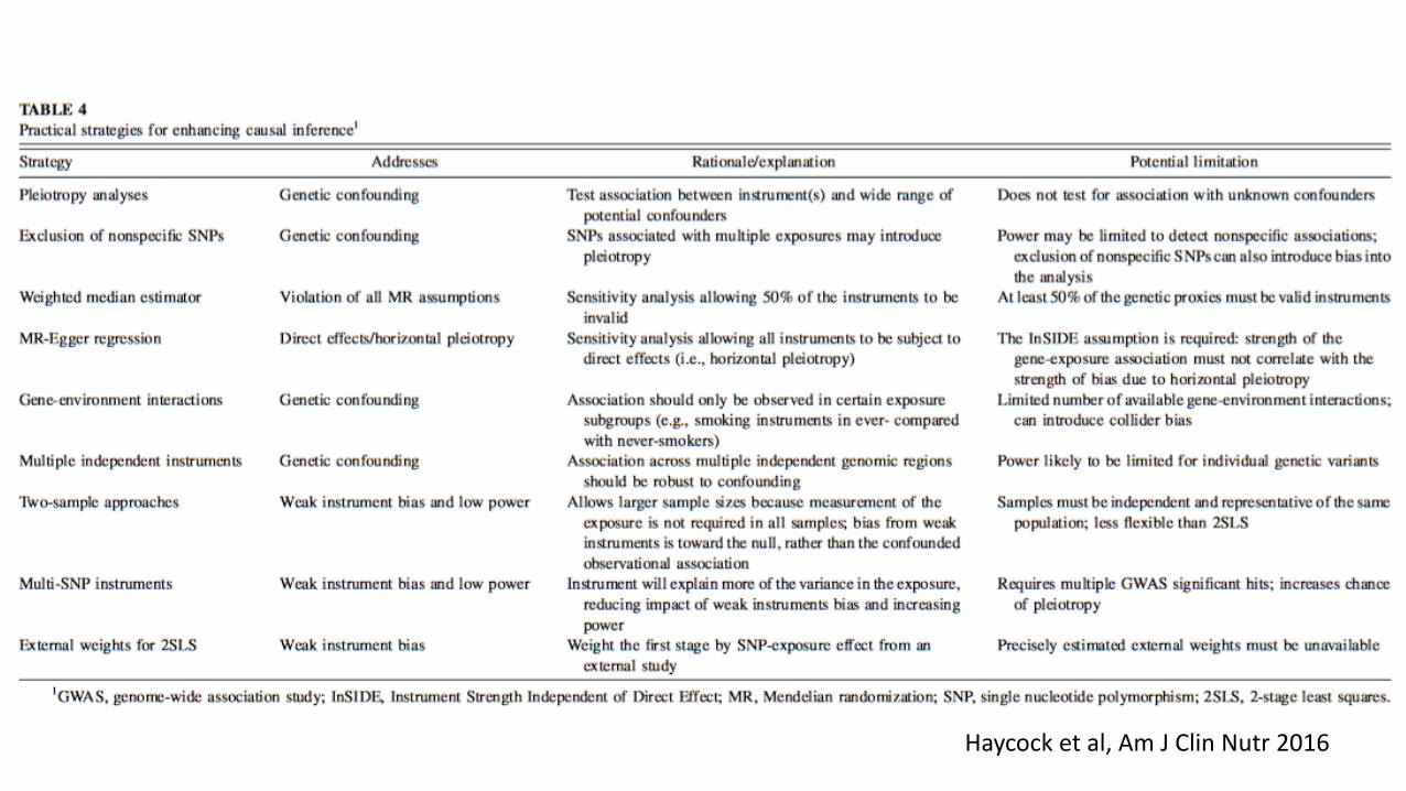
Haycock et al, Am J Clin Nutr 2016
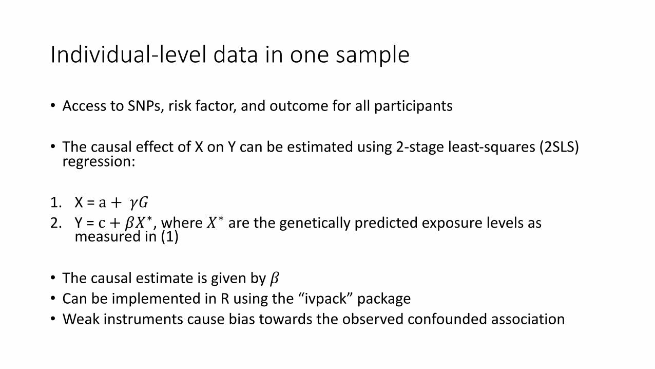
Individual-level data in one sample
• Access to SNPs, risk factor, and outcome for all participants
• The causal effect of X on Y can be estimated using 2-stage least-squares (2SLS) regression:
1. X = a + 𝛾𝐺2. Y = c + 𝛽𝑋∗, where 𝑋∗ are the genetically predicted exposure levels as
measured in (1)
• The causal estimate is given by 𝛽• Can be implemented in R using the “ivpack” package• Weak instruments cause bias towards the observed confounded association
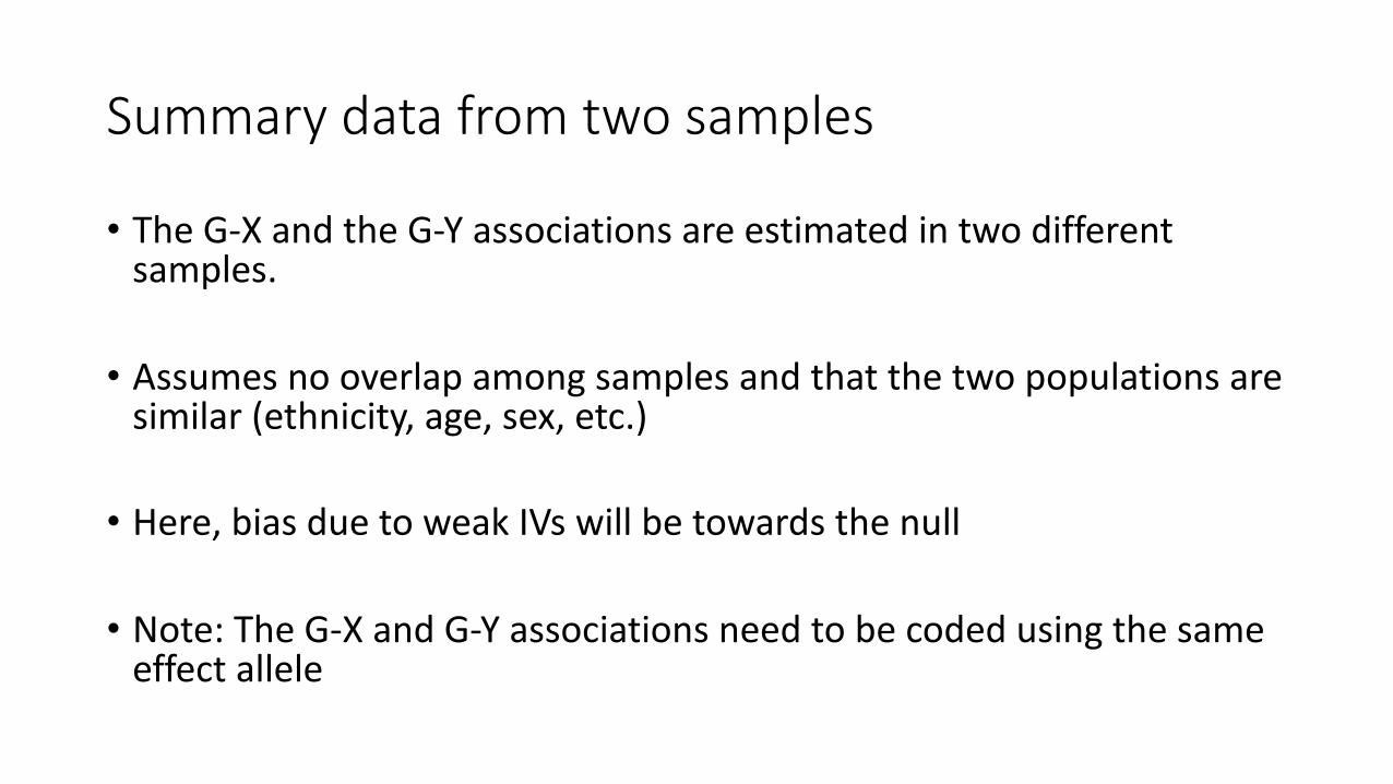
Summary data from two samples
• The G-X and the G-Y associations are estimated in two different samples.
• Assumes no overlap among samples and that the two populations are similar (ethnicity, age, sex, etc.)
• Here, bias due to weak IVs will be towards the null
• Note: The G-X and G-Y associations need to be coded using the same effect allele

Summary data from two samples
β̂ =β1kβ2kσβ2 k
−2
k∑
β1kσβ2 k
−2
k∑
se(β̂) = 1β1k2σβ2 k
−2
k∑
β1k is the mean change in X per allele for SNP k, β2k is the mean change in Y per allele for SNP k, 𝜎"#$" is the inverse variance for the G-Y association.
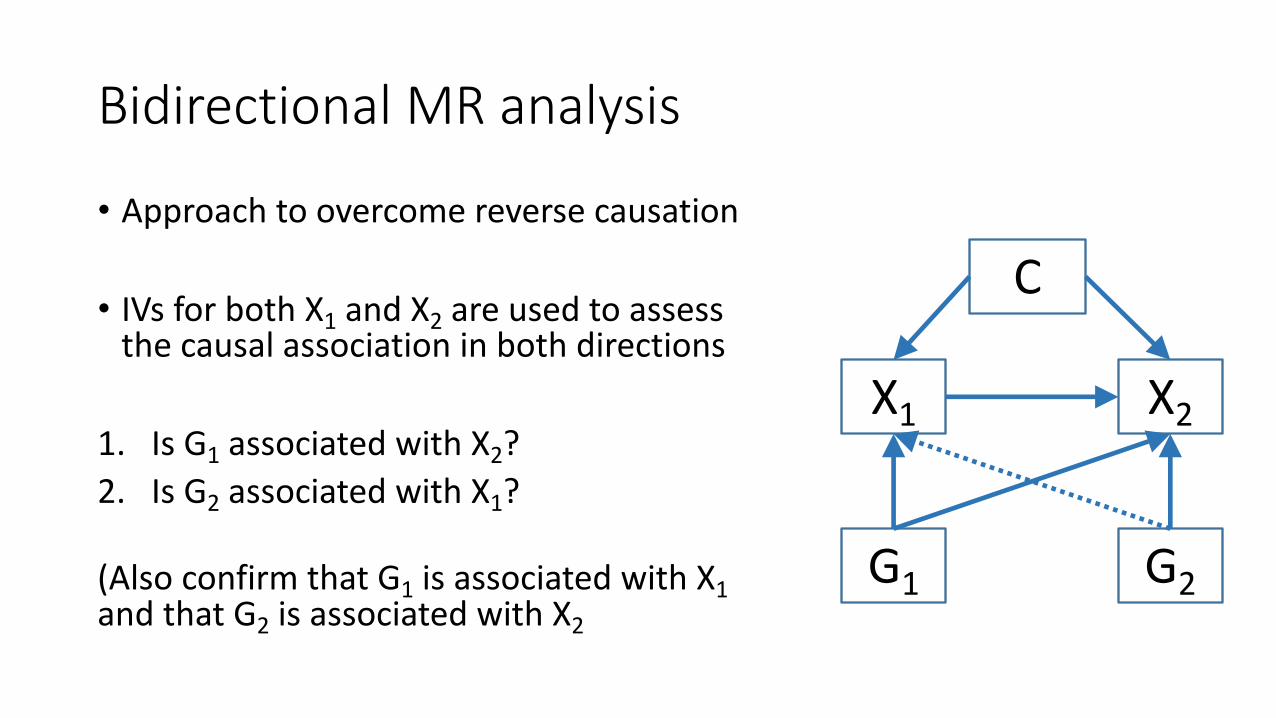
Bidirectional MR analysis
• Approach to overcome reverse causation
• IVs for both X1 and X2 are used to assess the causal association in both directions
1. Is G1 associated with X2?2. Is G2 associated with X1?
(Also confirm that G1 is associated with X1 and that G2 is associated with X2
X1 X2
G1 G2
C
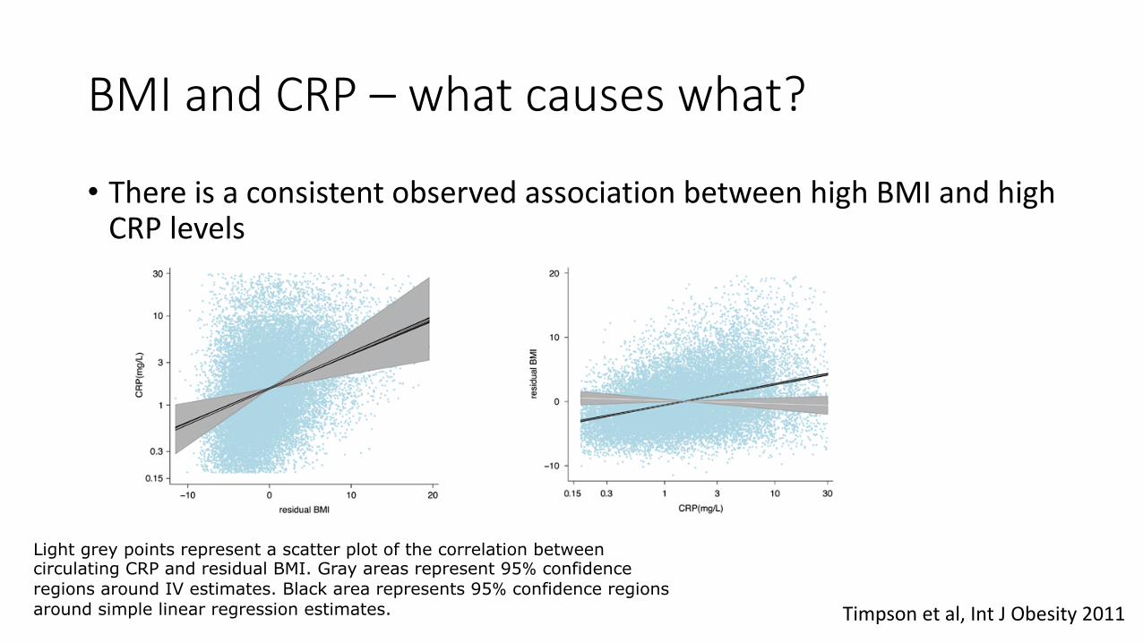
BMI and CRP – what causes what?
• There is a consistent observed association between high BMI and high CRP levels
Timpson et al, Int J Obesity 2011
Light grey points represent a scatter plot of the correlation between circulating CRP and residual BMI. Gray areas represent 95% confidence regions around IV estimates. Black area represents 95% confidence regions around simple linear regression estimates.
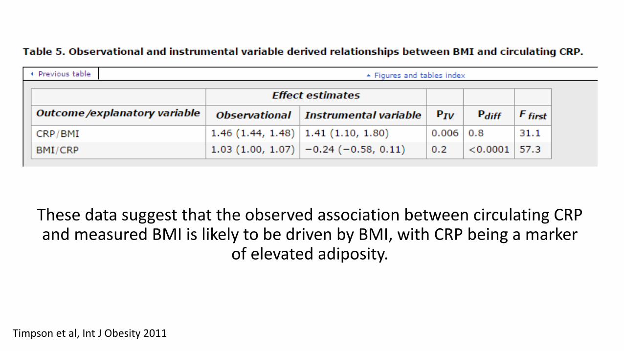
These data suggest that the observed association between circulating CRP and measured BMI is likely to be driven by BMI, with CRP being a marker
of elevated adiposity.
Timpson et al, Int J Obesity 2011
Drawbacks with MR analysis
• Large sample sizes are needed • As genetic effects on risk factors are typically small, MR estimates of
association have much wider confidence intervals than conventional epidemiological estimates.
• Make sure that the three key assumptions hold• In practice, this is very difficult, especially for the third assumption of no
pleiotropy.
Haycock et al, Am J Clin Nutr 2016
MR-base: An easy tool for Mendelian Randomization Analysis
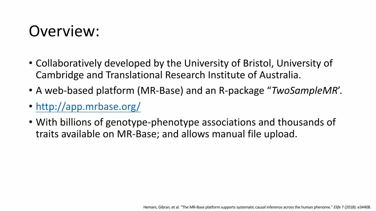
Overview:
• Collaboratively developed by the University of Bristol, University of Cambridge and Translational Research Institute of Australia.• A web-based platform (MR-Base) and an R-package “TwoSampleMR’.• http://app.mrbase.org/• With billions of genotype-phenotype associations and thousands of
traits available on MR-Base; and allows manual file upload.
Hemani, Gibran, et al. "The MR-Base platform supports systematic causal inference across the human phenome." Elife 7 (2018): e34408.

Accept the data access agreement;Log in with your Google ID
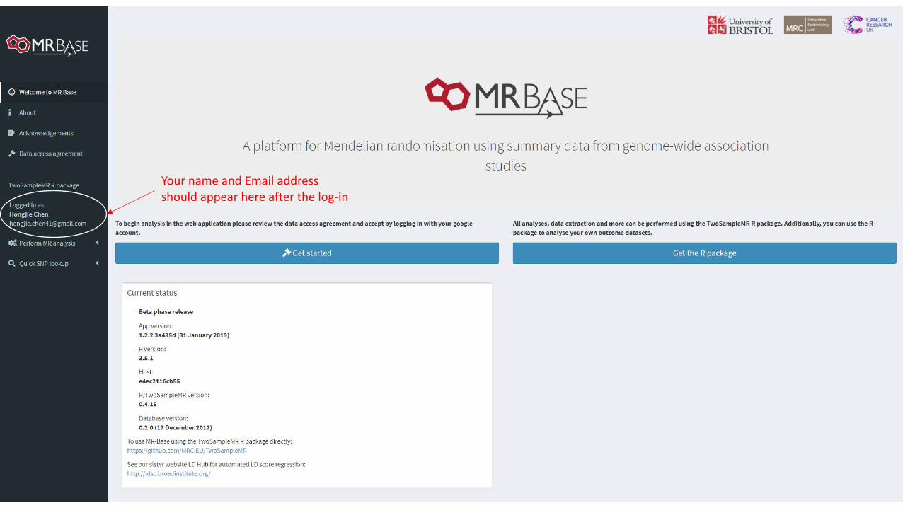
Your name and Email addressshould appear here after the log-in
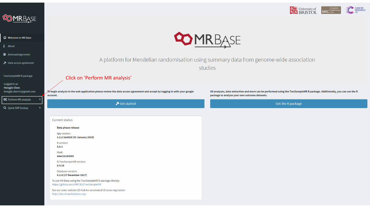
Click on ‘Perform MR analysis’
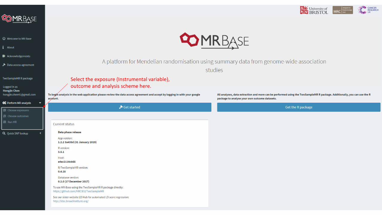
Select the exposure (Instrumental variable),outcome and analysis scheme here.
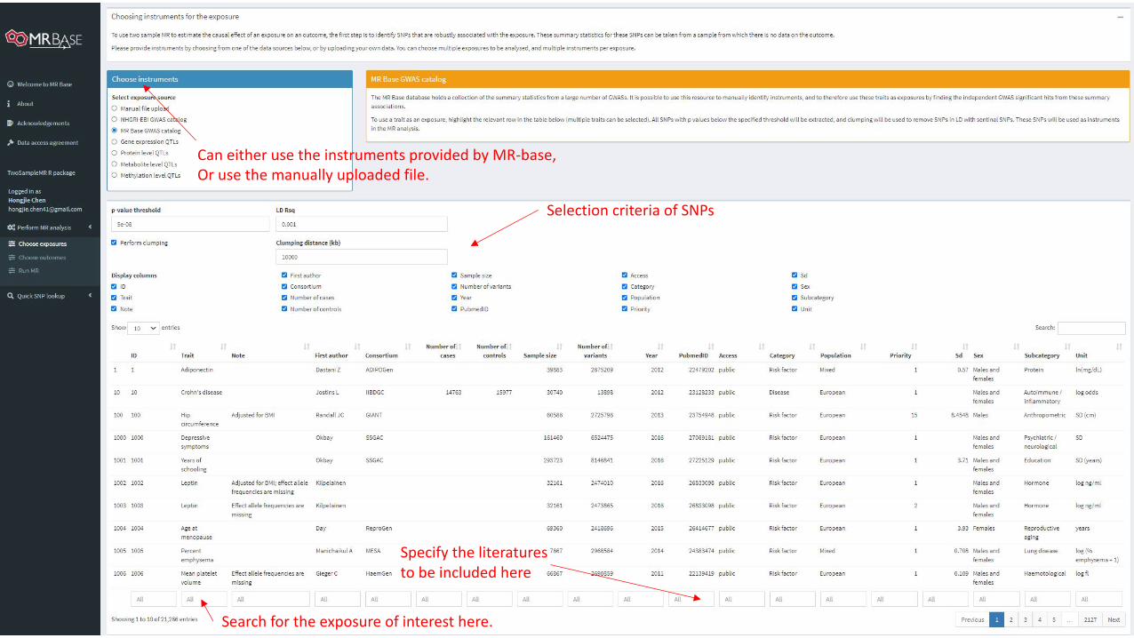
Can either use the instruments provided by MR-base,Or use the manually uploaded file.
Selection criteria of SNPs
Search for the exposure of interest here.
Specify the literatures to be included here
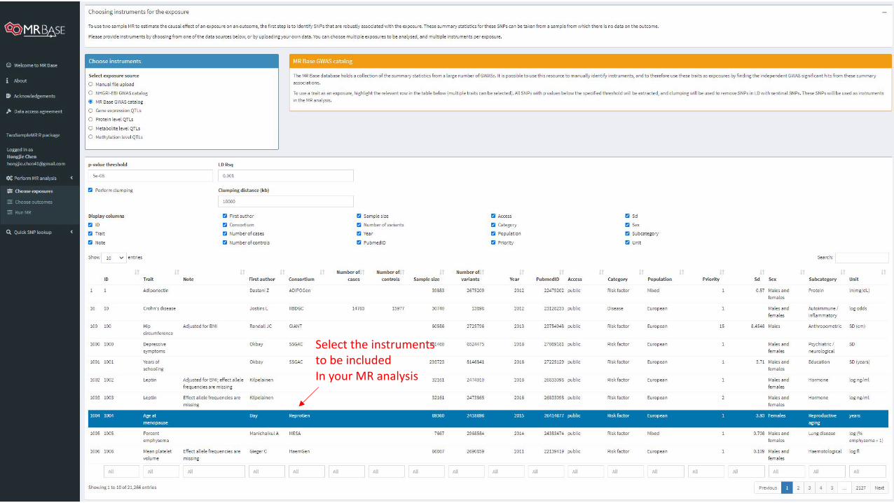
Select the instruments to be includedIn your MR analysis
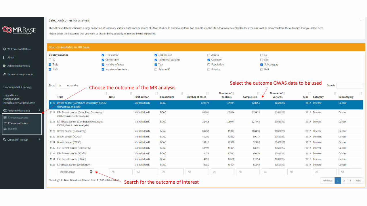
Choose the outcome of the MR analysis
Search for the outcome of interest
Select the outcome GWAS data to be used
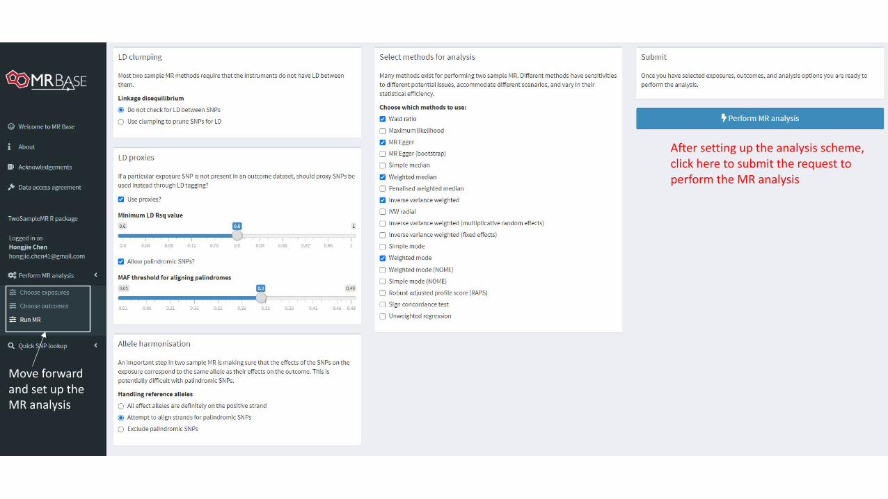
Move forward and set up theMR analysis
After setting up the analysis scheme,click here to submit the request to perform the MR analysis
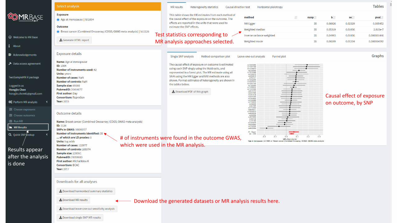
Results appearafter the analysisis done
# of instruments were found in the outcome GWAS,which were used in the MR analysis.
Test statistics corresponding to MR analysis approaches selected.
Causal effect of exposure on outcome, by SNP
Download the generated datasets or MR analysis results here.

Exercise• Explore MR-Base (http://www.mrbase.org) to conduct your own MR
study. • Run an MR study of age at menopause and breast cancer risk
following the example we showed in class. • Check out UK Biobank (https://www.ukbiobank.ac.uk), an amazing
resource for genetic epidemiological studies (~500,000 participants with GWAS and comprehensive phenotype data) .
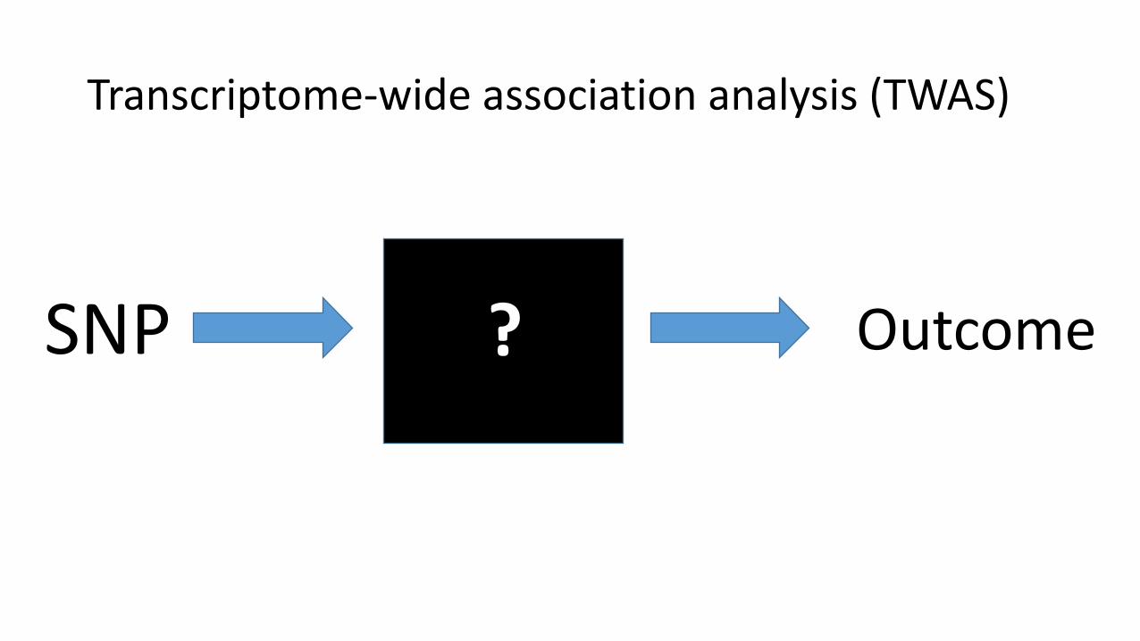
Transcriptome-wide association analysis (TWAS)
SNP ? Outcome
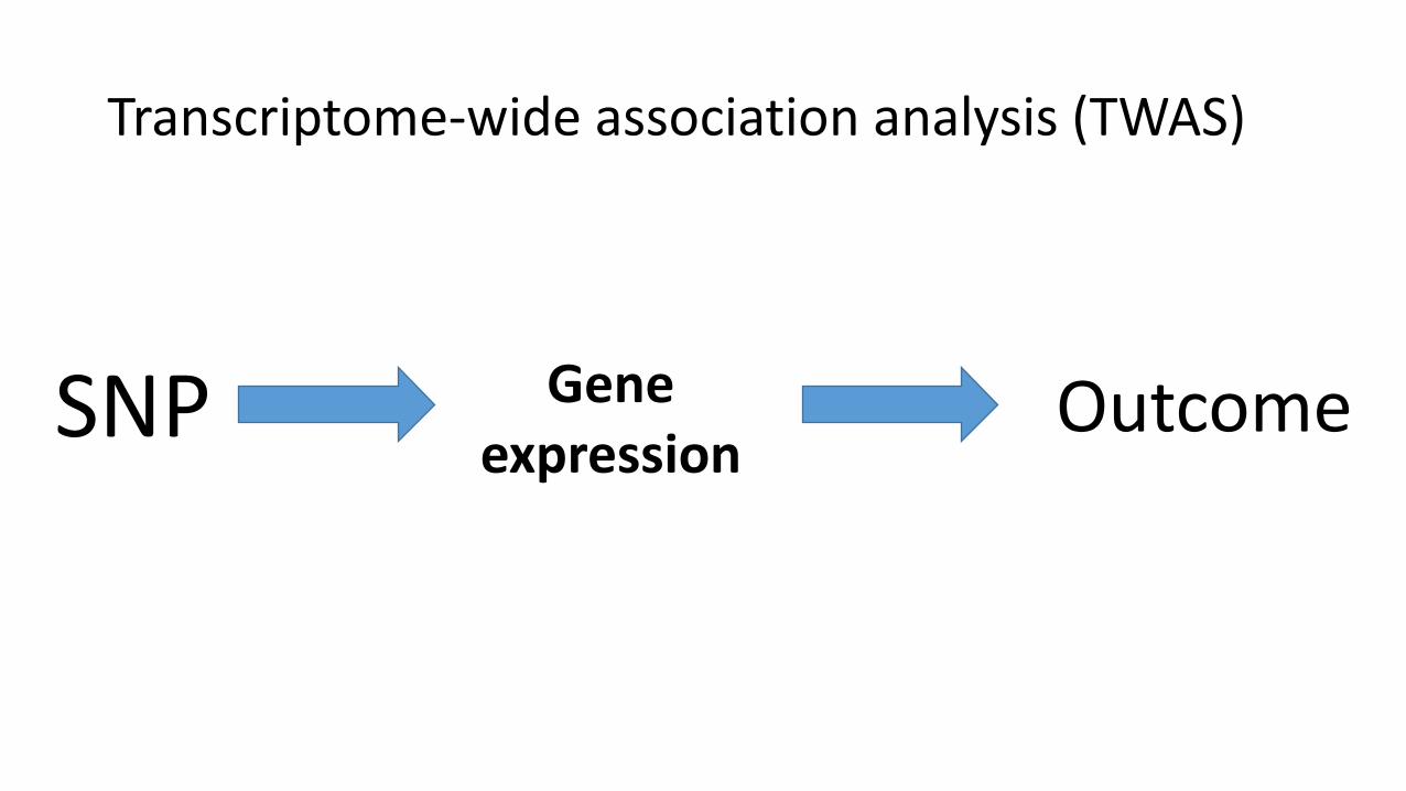
Transcriptome-wide association analysis (TWAS)
SNP Gene expression
Outcome
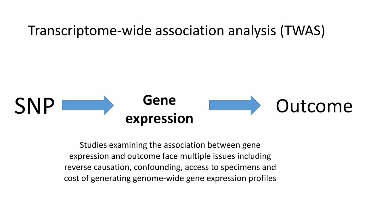
Transcriptome-wide association analysis (TWAS)
SNP Gene expression
Outcome
Studies examining the association between gene expression and outcome face multiple issues including
reverse causation, confounding, access to specimens and cost of generating genome-wide gene expression profiles
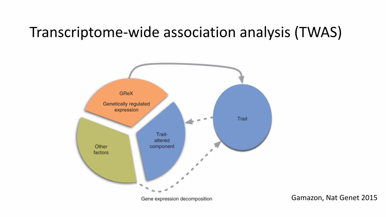
Transcriptome-wide association analysis (TWAS)
Gamazon, Nat Genet 2015
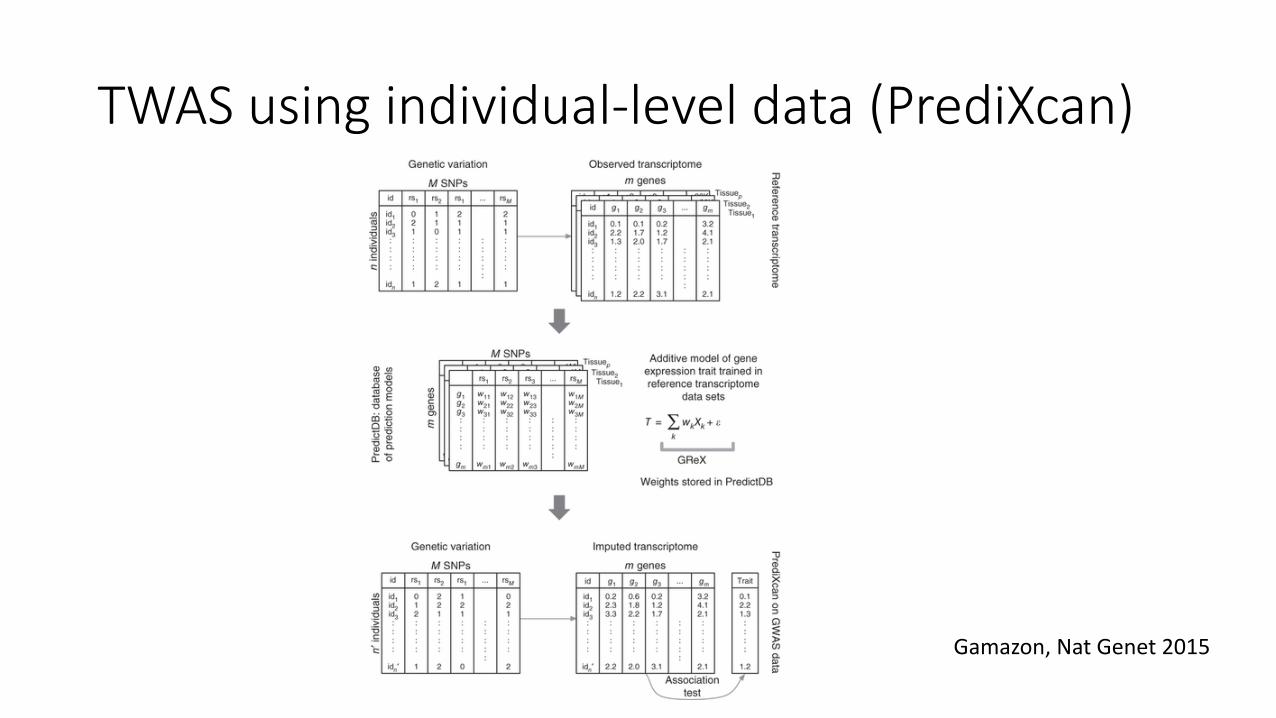
TWAS using individual-level data (PrediXcan)
Gamazon, Nat Genet 2015
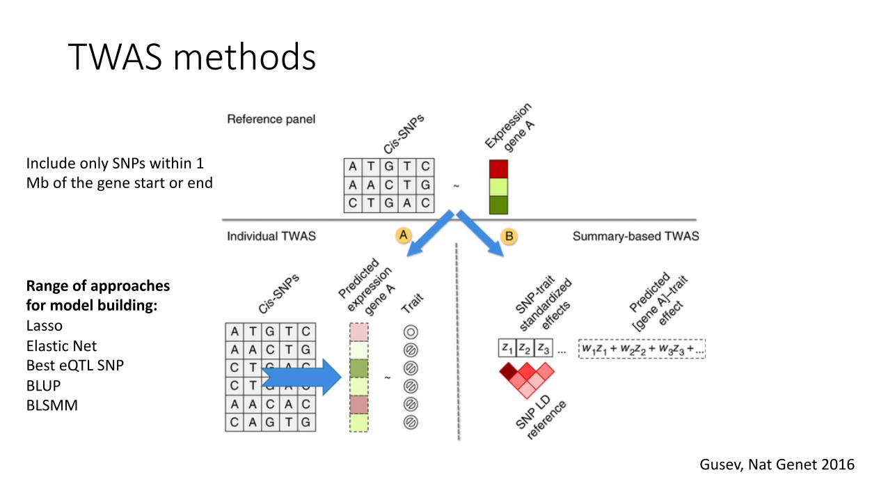
TWAS methods
Gusev, Nat Genet 2016
Include only SNPs within 1 Mb of the gene start or end
Range of approaches for model building:Lasso Elastic NetBest eQTL SNPBLUPBLSMM
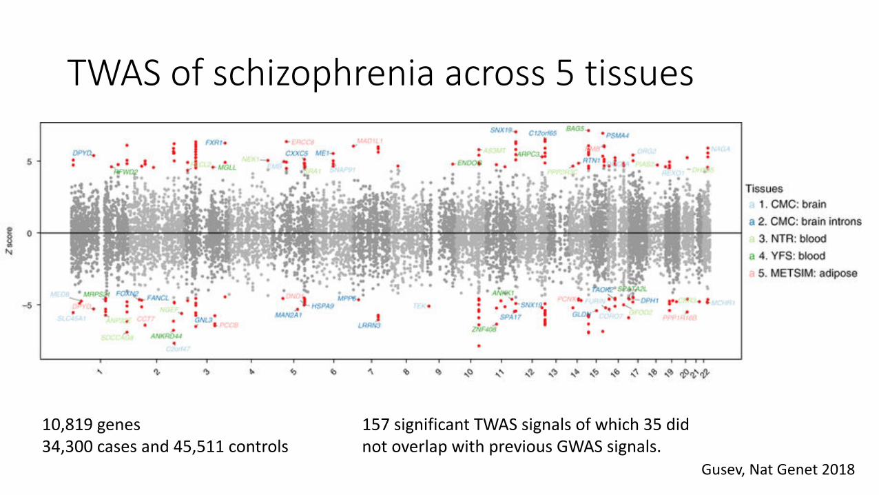
TWAS of schizophrenia across 5 tissues
Gusev, Nat Genet 2018
10,819 genes34,300 cases and 45,511 controls
157 significant TWAS signals of which 35 did not overlap with previous GWAS signals.
Module evaluation
• Please complete the online evaluation available by logging into your SISG account.
• After you complete the evaluation, you will be able to download your Certificate of Completion through the account.
• http://uwsurvey.qualtrics.com/jfe/form/SV_6A3uZcCSyPxMwfz
Recommended