CRANFIELD UNIVERSITY
Micheil Gordon
Integrated Fatigue Analysis of an Offshore Wind Turbine and
Monopile Foundation
School of Energy, Environment and Agrifood
Advanced Mechanical Engineering
MSc
Academic Year: 2014 - 2015
Supervisor: Professor Feargal Brennan
September 2015

CRANFIELD UNIVERSITY
School of Energy, Environment and Agrifood
Advanced Mechanical Engineering
MSc
Academic Year 2014 - 2015
Micheil Gordon
Integrated Fatigue Analysis of an Offshore Wind Turbine and
Monopile Foundation
Supervisor: Feargal Brennan
September 2015
This thesis is submitted in partial fulfilment of the requirements for
the degree of Advanced Mechanical Engineering
© Cranfield University 2015. All rights reserved. No part of this
publication may be reproduced without the written permission of the
copyright owner.


i
ABSTRACT
Fatigue is a major concern for the design of offshore wind turbines with monopile
foundations as a result of the very high number of cyclic loads the system
experiences over its lifetime. This investigation presents a numerical model in
Matlab capable of performing an integrated wind and wave loading fatigue
analysis of an offshore wind turbine and monopile foundation. Subsequently the
model has been used to explore how different wind and wave superposition
methodologies effect the final system fatigue life. The results were found to agree
with the literature and indicated that there is no difference between using the out-
of-phase spectral superposition or Kühn’s unweighted equivalent method when
rounded to one decimal place. Full explanations and discussions are provided
throughout.
Keywords:
Morison Equation, Wave Theories, Time Domain, Frequency Domain, Fourier
Transform, Actuator Disk Theory, Mudline Bending Stress, Power Spectra
Density, Damage Equivalent Stress Range


iii
ACKNOWLEDGEMENTS
Firstly, I would like to express my sincere gratitude to my thesis supervisor
Professor Feargal Brennan who despite his busy schedule, always found time to
sit down and discuss my concerns whenever I was in need. I would also like to
thank two of my student colleagues, Marc and Emily for their continued help with
some of the more advanced mathematics used in the study. And finally thank you
to my girlfriend and family for mental and financial support over the last year,
which without, this would have never been possible.

v
TABLE OF CONTENTS
ABSTRACT ......................................................................................................... i
ACKNOWLEDGEMENTS................................................................................... iii
LIST OF FIGURES ............................................................................................ vii
LIST OF TABLES ............................................................................................... ix
LIST OF EQUATIONS ........................................................................................ x
LIST OF ABBREVIATIONS .............................................................................. xiii
1 INTRODUCTION ............................................................................................. 1
1.1 Offshore Wind Turbine Fatigue ................................................................. 3
1.2 Fatigue Analysis Methods ......................................................................... 4
1.2.1 Miner’s Rule ....................................................................................... 5
1.2.2 Deterministic Method.......................................................................... 6
1.2.3 Time Domain ...................................................................................... 6
1.2.4 Frequency Domain ............................................................................. 8
1.3 Aim and Objectives ................................................................................. 10
2 METHODOLOGY .......................................................................................... 11
2.1 Methodology Overview Flowchart ........................................................... 12
2.2 Reference Parameters ............................................................................ 13
2.2.1 Reference Site Conditions ................................................................ 13
2.2.2 Reference Wind Turbine and Foundation Parameters ..................... 14
2.3 Wave Loading ......................................................................................... 17
2.3.1 Wave Climate ................................................................................... 17
2.3.2 Wave Spectra ................................................................................... 18
2.3.3 Wave Kinematics ............................................................................. 22
2.3.4 Airy Linear Wave Theory .................................................................. 23
2.3.5 Stokes Second Order Wave Theory ................................................. 26
2.3.6 Morison Equation ............................................................................. 26
2.4 Wind Loading .......................................................................................... 29
2.4.1 Wind Climate .................................................................................... 29
2.4.2 Normal Wind Conditions ................................................................... 29
2.4.3 Wind Modelling ................................................................................. 30
2.5 System Response from Wind Loading .................................................... 36
2.5.1 Tower Top Displacement Transfer Function .................................... 38
2.6 System Response from Wave Loading ................................................... 41
2.6.1 MWL Displacement Transfer Function ............................................. 41
2.7 Mudline Bending Stress from Wind ......................................................... 44
2.7.1 Mudline Wind Bending Stress Transfer Function ............................. 44
2.7.2 Power Spectral Density of the Turbulent Thrust Force on the Rotor
.................................................................................................................. 45
2.7.3 Mudline Bending Stress Spectrum from Wind Loading .................... 46
2.7.4 Mudline Bending Stress Time Series ............................................... 49
vi
2.8 Mudline Bending Stress from Wave ........................................................ 52
2.8.1 Mudline Wave Bending Stress Transfer Function ............................ 52
2.8.2 Power Spectral Density of Wave Loading ........................................ 53
2.8.3 Mudline Bending Stress Spectrum from Wave Loading ................... 55
2.8.4 Mudline Bending Stress Time Series ............................................... 57
2.9 Rainflow Counting and Damage Equivalent Stress Range ..................... 59
2.10 Wind and Wave Loading Superposition ................................................ 60
3 RESULTS ...................................................................................................... 61
3.1 Sensitivity Analyses ................................................................................ 61
3.2 Superposition of the Wind and Wave Stresses Before and After
Rainflow Counting ......................................................................................... 62
3.3 Summary of Results ................................................................................ 63
4 DISCUSSION ................................................................................................ 65
4.1 Evaluating Airy and Stokes Second Order Wave Theories ..................... 65
4.2 Significance of the Drag Term in the Morison Equation .......................... 67
4.3 Fatigue Loading Regimes ....................................................................... 68
4.4 Results .................................................................................................... 69
4.4.1 Simulation Length ............................................................................ 70
4.4.2 Spectral Multiplication ...................................................................... 70
4.4.3 System Response ............................................................................ 71
4.4.4 Final Results Analysis ...................................................................... 71
4.5 Areas for Future Investigations ............................................................... 74
5 CONCLUSIONS ............................................................................................ 75
REFERENCES ................................................................................................. 77
APPENDICES .................................................................................................. 81
Appendix A UK Significant Wave Heights ..................................................... 81
Appendix B Equations for Airy Linear and Stoke’s 2nd Order Wave Theories
...................................................................................................................... 82
Appendix C Integration of Airy Linear Wave Theory over Depth ................... 83
Appendix D Integration of Stoke’s 2nd Order Wave Theory over Depth ........ 87
Appendix E Actuator Disk Theory ................................................................. 89
Appendix F Wind Turbulence Intensity Factor .............................................. 91
Appendix G Wind Speed Distribution ............................................................ 92
Appendix H Wind Turbulence ....................................................................... 97
Appendix I Finding the Tower Top Stiffness ............................................... 104
Appendix J Finding the MWL Stiffness ....................................................... 105
Appendix K Mudline Wind Bending Stress Transfer Function ..................... 108
Appendix L Turbulent Thrust Force PSD .................................................... 110
Appendix M List of S-N Curves ................................................................... 112
vii
LIST OF FIGURES
Figure 1: Global wind power (Gsanger and Pitteloud, 2013) .............................. 1
Figure 2: S-N curves for steel structures in seawater with cathodic protection (Det Norske Veritas, 2012) .................................................................................. 5
Figure 3: Time based fatigue determination of fatigue damage from wave loading (Passon, 2015) ............................................................................................ 7
Figure 4: Methodology flow chart ..................................................................... 12
Figure 5: Offshore wind activity in Europe (Lynn, 2011) ................................... 13
Figure 6: Wave spectra .................................................................................... 20
Figure 7: Free surface elevation time series from JONSWAP spectrum .......... 22
Figure 8: Ranges of validity for a variety of wave theories (Det Norske Veritas, 2014) ......................................................................................................... 23
Figure 9: Water particle motion (Veldkamp and Van Der Tempel, 2005) ......... 24
Figure 10: Actuator disk model (Manwell et al., 2009) ...................................... 30
Figure 11: Number of occurrences of 10min wind speed intervals in one year with wind speed bins 1m/s wide ........................................................................ 33
Figure 12: Kaimal spectrum for mean wind speed from 3.5m/s to 24.5m/s and with a turbulence intensity of 12% ............................................................. 35
Figure 13: Offshore wind system modelled as a 1 degree of freedom mass-on-pole system (Van Der Tempel, 2006) ........................................................ 36
Figure 14: Transfer function of tower top displacement for the NREL reference turbine with its respective foundation properties (peak=0.6330Hz) ........... 40
Figure 15: Transfer function of MWL displacement for the NREL reference turbine with its respective foundation properties (peak=8.1652Hz) ....................... 42
Figure 16: Transfer function for mudline bending stress from wind loading ..... 44
Figure 17: PSDs of the turbulent thrust force on the rotor at each operational mean wind speed with a 12% turbulence intensity .................................... 46
Figure 18: Process to find the mudline bending stress spectrum from wind loading .................................................................................................................. 48
Figure 19: Mudline bending stress Spectrum from wind loading ...................... 49
Figure 20: Mudline bending stress for 10min mean wind speed of 10.5m/s ..... 51
Figure 21: Transfer function for mudline bending stress from wave loading .... 53
Figure 22: PSD of the wave loading integrated over the depth ........................ 55
viii
Figure 23: Process to find the mudline bending stress from wave loading ....... 56
Figure 24: Mudline bending stress Spectrum from wave loading ..................... 57
Figure 25: Mudline bending stress from wave loading ..................................... 58
Figure 26: Comparing results using Airy and Stokes 2nd order wave theories .. 66
Figure 27: Significance of the Drag term in the Morison Equation (no marine growth) ....................................................................................................... 67
Figure 28: Significance of the Drag term in the Morison Equation (with marine growth) ....................................................................................................... 68
Figure 29: In-phase versus out of phase superposition (Kühn, 2001) .............. 72
Figure 30: Significant wave height around the UK (ABP mer, 2008) ................ 81
Figure 31: Airy and Stoke’s 2nd order wave theories (Det Norske Veritas, 2010) .................................................................................................................. 82
Figure 32: Turbulence intensity as a function of mean wind speed (Van Der Tempel, 2006) ........................................................................................... 91
Figure 33: Turbulence intensity as a function of mean wind speed (Burton et al., 2011) ......................................................................................................... 91
Figure 34: Weibull probability density function when 𝑼 = 6m/s (Manwell et al., 2009) ......................................................................................................... 93
Figure 35: Yearly average wind speed at 100m elevation in European waters (Van Der Tempel, 2006) ............................................................................ 94
Figure 36: Weibull distribution for mean annual wind speed = 10m/s and SD=4.8 .................................................................................................................. 95
Figure 37: Example of the wind spped probability for a 1m/s wind speed bin (Lynn, 2011) ......................................................................................................... 95
Figure 38: Ten minute mean wind speed from 0.5m/s to 9.5m/s with turbulence superimposed on top ................................................................................. 98
Figure 39: Ten minute mean wind speed from 10.5m/s to 19.5m/s with turbulence superimposed on top ................................................................................. 99
Figure 40: Ten minute mean wind speed from 20.5m/s to 29.5m/s with turbulence superimposed on top ............................................................................... 100
Figure 41: One month of wind speed data ..................................................... 101
Figure 42: Wind loading over a one month period .......................................... 103
Figure 43: Finding the tower top displacement transfer function .................... 104
ix
LIST OF TABLES
Table 1: Site reference parameters .................................................................. 14
Table 2: Turbine and foundation reference parameters ................................... 16
Table 3: Wave parameters (Det Norske Veritas, 2010, Van Der Tempel, 2006) .................................................................................................................. 18
Table 4: Wave number determination using two methods ................................ 26
Table 5: Finding the tower top stiffness ............................................................ 39
Table 6: Sensitivity analysis ............................................................................. 61
Table 7: Results summary table ....................................................................... 64
Table 8: Finding the axial induction factor for a turbine with a Cp=0.482 ......... 89
Table 9: Turbine thrust calculation parameters .............................................. 102
Table 10: S-N curves for most frequently used structural details – Reproduced from DNV-J101 (Det Norske Veritas, 2014) ............................................. 112

x
LIST OF EQUATIONS
Equation 1: Miners Rule ..................................................................................... 6
Equation 2: Pierson-Moskowitz wave spectrum ............................................... 19
Equation 3: JONSWAP wave spectrum ........................................................... 19
Equation 4: Normalizing factor ......................................................................... 19
Equation 5: Peak Period ................................................................................... 19
Equation 6: Peak frequency ............................................................................. 19
Equation 7: Spectral width parameter .............................................................. 19
Equation 8: Wave amplitude components ........................................................ 21
Equation 9: Free surface elevation ................................................................... 21
Equation 10: Horizontal water particle velocity (Airy) ....................................... 24
Equation 11: Horizontal water particle acceleration (Airy) ................................ 24
Equation 12: Wave number .............................................................................. 24
Equation 13: Wave length (for Airy shallow water and Stokes 2nd order) ......... 25
Equation 14: Wave celerity (for Airy shallow water and Stokes 2nd order) ........ 25
Equation 15: Wave celerity (for Airy deep water) ............................................. 25
Equation 16: Dispersion relation ....................................................................... 25
Equation 17: Morison Equation ........................................................................ 27
Equation 18: Thrust - Wind turbine ................................................................... 31
Equation 19: Axial induction factor ................................................................... 31
Equation 20: Turbulence Intensity .................................................................... 34
Equation 21: Equation of motion ...................................................................... 37
Equation 22: Frequency response function for displacement ........................... 37
Equation 23: Undamped natural frequency ...................................................... 37
Equation 24: Damping ratio .............................................................................. 38
Equation 25: Damping coefficient ..................................................................... 38
Equation 26: Frequency response function for displacement ........................... 38
Equation 27: Transfer function for the tower top displacement......................... 40
Equation 28: Transfer function for the MWL displacement ............................... 42
xi
Equation 29: Transfer function for mudline bending stress from wind loading.. 45
Equation 30: Definition of PSD (1) .................................................................... 46
Equation 31: Definition of PSD (2) .................................................................... 47
Equation 32: Response spectrum of the mudline bending stress from wind loading ....................................................................................................... 47
Equation 33: Phasor form of a complex number .............................................. 50
Equation 34: Transfer function for mudline bending stress from wave loading 52
Equation 35: PSD wave loading integrated over depth .................................... 54
Equation 36: Response spectrum of the mudline bending stress from wind loading ....................................................................................................... 55
Equation 37: Damage equivalent stress range using Kühn’s unweighted equivalent method ..................................................................................... 62
Equation 38: Damage equivalent stress range direct superposition ................. 63
Equation 39: SN curve ..................................................................................... 63
Equation 40: Power coefficient (1) .................................................................... 89
Equation 41: Rotor power ................................................................................. 89
Equation 42: Power coefficient (2) .................................................................... 89
Equation 43: Weibull probability distribution ..................................................... 92
Equation 44: Shape factor ‘k’............................................................................ 92
Equation 45: Scale factor ‘c’ ............................................................................. 92
Equation 46: Kaimal spectrum .......................................................................... 97
Equation 47: Integral scale parameter .............................................................. 97
Equation 48: Differential equation of the elastic curve .................................... 105
Equation 49: Moment ..................................................................................... 105
Equation 50: Equation of the elastic curve ..................................................... 105
Equation 51: Differential equation of the elastic curve .................................... 106
Equation 52: Simplified equation of the elastic curve where z=h .................... 106
Equation 53: Stiffness .................................................................................... 106
Equation 54: Stiffness at hub height ............................................................... 107
Equation 55: Stiffness at the MWL (1) ............................................................ 107
Equation 56: Stiffness at the MWL (2) ............................................................ 107
xii
Equation 57: Flexure Formula (1) (Gere and Goodno, 2009) ......................... 108
Equation 58: Flexure Formula (2) ................................................................... 108
Equation 59: Deflection as a function of height .............................................. 108
Equation 60: Bending stress in terms of displacement ................................... 108
Equation 61: Transfer function for mudline bending stress from wind loading 109
Equation 62: PSD of the turbulent thrust force on the rotor ............................ 110
Equation 63: Normalised Kaimal spectrum .................................................... 110
Equation 64: Ten minute wind speed standard deviation (from Equation 20) 110
Equation 65: Thrust coefficient estimation (Frohboese et al., 2010) ............... 111
xiii
LIST OF ABBREVIATIONS
BEM Blade Element Momentum Theory
DAF Dynamic Amplification Factor
DNV Det Norske Veritas
EEA European Environmental Agency
EWEA European Wind Energy Association
FFT Fast Fourier Transform
IFFT Inverse Fast Fourier Transform
JONSWAP Joint North Sea Wave Project
MWL Mean Water Level
NREL National Renewable Energy Laboratory
OWT Offshore Wind Turbine
PSD Power Spectral Density
RFC Rainflow Counting
TLP Tension Leg Platform

xiv

1
1 INTRODUCTION
Worldwide renewable energy production has been increasing in recent years as
governments strive to meet environmental legislation, curtail dependence on
fossil fuel derived energy, address issues surrounding climate change as well as
lower CO2 emissions (Breton and Moe, 2009). Both onshore and offshore global
wind energy generation has witnessed yearly increases. In 1997 the total global
installed capacity was 7.5GW which rose, in 2012, to more than 282GW (refer to
Figure 1), and now represents a major contributor in the global electricity
production infrastructure (Gsanger and Pitteloud, 2013).
Figure 1: Global wind power (Gsanger and Pitteloud, 2013)
The wind energy sector in Europe currently have the largest installed wind power
generation capacity of any continent amounting to 128.8GW (EWEA, 2015).
However, Europe’s dominant position is being challenged by the Asian wind
energy markets driven by rapid expansion in China. In 2012 there were almost
100GW of installed capacity across the Asian continent (Gsanger and Pitteloud,
2013) and according to the World Wind Energy Association, by 2016, the global
wind energy capacity will reach 500GW and by 2020, 1000GW (Gsanger and
Pitteloud, 2013).
2
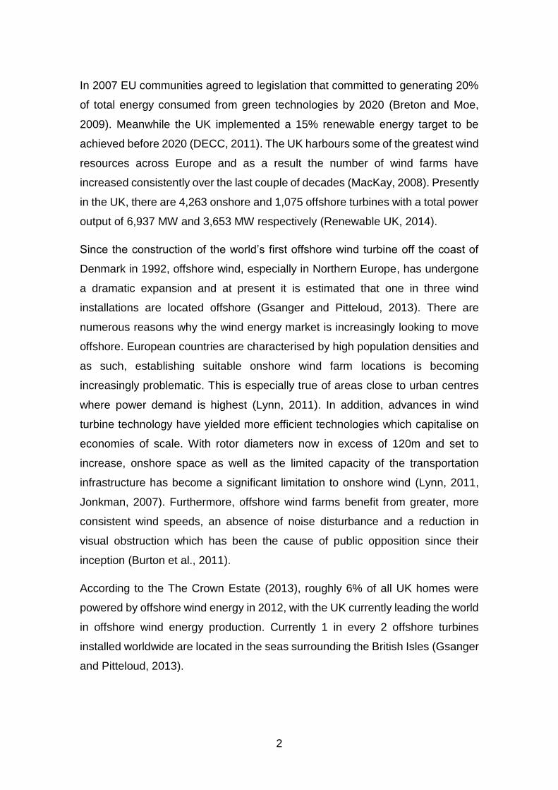
In 2007 EU communities agreed to legislation that committed to generating 20%
of total energy consumed from green technologies by 2020 (Breton and Moe,
2009). Meanwhile the UK implemented a 15% renewable energy target to be
achieved before 2020 (DECC, 2011). The UK harbours some of the greatest wind
resources across Europe and as a result the number of wind farms have
increased consistently over the last couple of decades (MacKay, 2008). Presently
in the UK, there are 4,263 onshore and 1,075 offshore turbines with a total power
output of 6,937 MW and 3,653 MW respectively (Renewable UK, 2014).
Since the construction of the world’s first offshore wind turbine off the coast of
Denmark in 1992, offshore wind, especially in Northern Europe, has undergone
a dramatic expansion and at present it is estimated that one in three wind
installations are located offshore (Gsanger and Pitteloud, 2013). There are
numerous reasons why the wind energy market is increasingly looking to move
offshore. European countries are characterised by high population densities and
as such, establishing suitable onshore wind farm locations is becoming
increasingly problematic. This is especially true of areas close to urban centres
where power demand is highest (Lynn, 2011). In addition, advances in wind
turbine technology have yielded more efficient technologies which capitalise on
economies of scale. With rotor diameters now in excess of 120m and set to
increase, onshore space as well as the limited capacity of the transportation
infrastructure has become a significant limitation to onshore wind (Lynn, 2011,
Jonkman, 2007). Furthermore, offshore wind farms benefit from greater, more
consistent wind speeds, an absence of noise disturbance and a reduction in
visual obstruction which has been the cause of public opposition since their
inception (Burton et al., 2011).
According to the The Crown Estate (2013), roughly 6% of all UK homes were
powered by offshore wind energy in 2012, with the UK currently leading the world
in offshore wind energy production. Currently 1 in every 2 offshore turbines
installed worldwide are located in the seas surrounding the British Isles (Gsanger
and Pitteloud, 2013).
3
Despite their merits, offshore wind is subject to approximately one and a half to
two times greater financial costs than their onshore counterparts, are currently
limited to shallow waters below 30m of depth (Breton and Moe, 2009), and are
subjected to additional wave and current loads (Jonkman, 2007).
The augmented costs borne by offshore wind are attributed to installation and
maintenance, the logistics of subsea cabling to establish grid connectivity, as well
as the required complex foundation systems (EEA, 2009). According to the
European Environmental Agency (EEA) the cost of the offshore foundation
amounts to as much as 15% to 30% of the overall investment depending on the
water depth (EEA, 2009) and Greenpeace, (2000) cited in EEA (2009) found that
a depth increase from 8m to 16m resulted in a rise of 11% in foundation cost.
In the future, it is predicted that offshore wind turbine near shore site availability
will diminish pushing offshore wind turbines into sites with deeper waters and
harsher conditions. In response, the industry is investigating a number of
foundation solutions such as the tripod and jacked foundation as well as floating
options such as tension leg platforms (TLP’s), spar buoy’s and semi-
submersibles. For more information refer to Jonkman (2007). However in the
short to medium term it is imperative that design of the monopile foundation is as
cost efficient as possible and that fatigue damage as a result of the wind and
wave interactions is adequately designed for, resulting in an economical structure
that is fit for purpose for its entire design life (Lynn, 2011).
The proceeding section will consider the importance of fatigue in the design of
offshore wind turbines and monopile foundations, and some of the techniques
that have been developed to ensure adequate fatigue lives are achieved.
1.1 Offshore Wind Turbine Fatigue
Offshore wind turbine design requires the consideration of two fundamental
aspects that must be evaluated during the design process. The first is the ability
of the system to withstand the ultimate loading conditions likely to occur, and the
second is the ability of the system to withstand the continuous cyclic loading
which lead to accumulated fatigue damage (Manwell et al., 2009). This
4
investigation is concerned with the more complex of the two, the fatigue of the
system.
Fatigue is caused by the repeated loading and unloading of a material resulting
in the formation of tiny internal cracks which propagate with every additional
loading cycle. Crack initiation is a result of the presence of small material defects
from manufacturing processes or from areas experiencing stress concentrations
(Patel, 1989).
Fatigue is a major concern for the design of offshore wind turbines (OWT) with
monopile foundations as a result of the very high number of cyclic loads the
system experiences over its lifetime. Under constant loading conditions, it is
assumed that a component able to endure 107 cycles will never fail from fatigue.
However, a typical wind turbine system can experience in excess of 108 cycles
over a 20 year lifetime (Burton et al., 2011). In addition, the slender shape and
form of the offshore wind turbine results in a system natural frequency that is very
close to the excitation frequencies from the wind, wave and mechanical loading
conditions (Arany et al., 2014). Thus, for reasons discussed, the design of OWT’s
are predominantly governed by fatigue rather than the ultimate load (Burton et
al., 2011, Dong et al., 2011), which in turn, is predominantly governed by wind
and wave loading (Passon and Branner, 2014). Therefore detailed fatigue
analyses, that take wind and wave loading into consideration, must be conducted
to enable adequate design concessions to ensure a system is fit for purpose
(Manwell et al., 2009). A number of the procedures used in OWT fatigue analyses
are presented below.
1.2 Fatigue Analysis Methods
There are currently three established methods used in the fatigue analysis of
offshore structures. These include the deterministic method, the time domain
method and the frequency domain method. Each method will be briefly
considered in the following sections.
5
1.2.1 Miner’s Rule
Empirical fatigue investigations usually involve the application of cyclic loads to
test specimens under constant load amplitudes (Pook, 2007). The purpose of
such experiments is to establish the number of loading cycles a specimen can
withstand at that constant amplitude until failure occurs. The test data is then
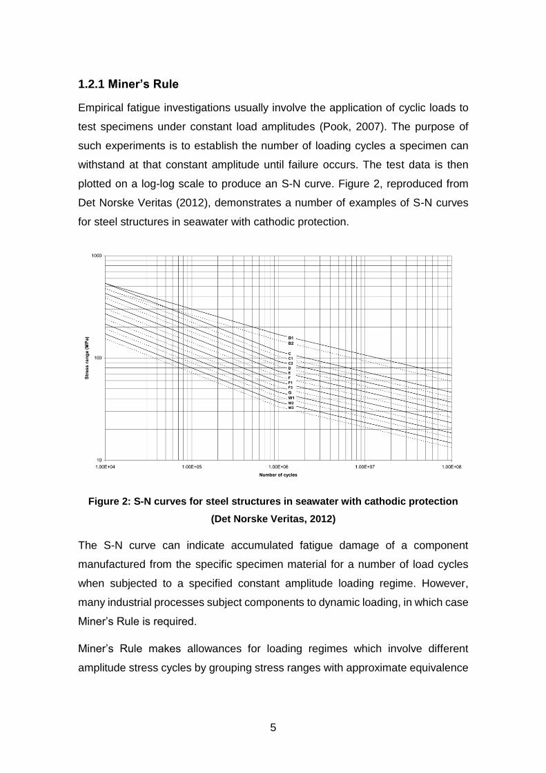
plotted on a log-log scale to produce an S-N curve. Figure 2, reproduced from
Det Norske Veritas (2012), demonstrates a number of examples of S-N curves
for steel structures in seawater with cathodic protection.
Figure 2: S-N curves for steel structures in seawater with cathodic protection
(Det Norske Veritas, 2012)
The S-N curve can indicate accumulated fatigue damage of a component
manufactured from the specific specimen material for a number of load cycles
when subjected to a specified constant amplitude loading regime. However,
many industrial processes subject components to dynamic loading, in which case
Miner’s Rule is required.
Miner’s Rule makes allowances for loading regimes which involve different
amplitude stress cycles by grouping stress ranges with approximate equivalence
6
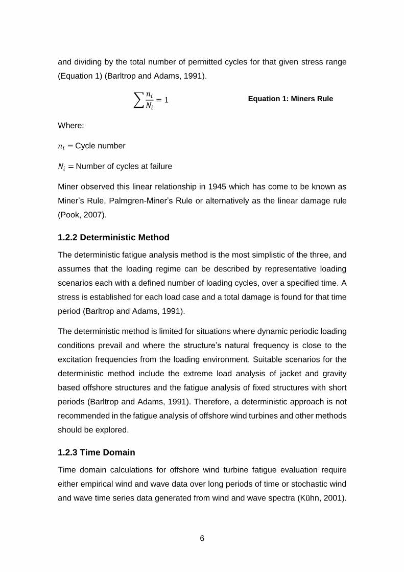
and dividing by the total number of permitted cycles for that given stress range
(Equation 1) (Barltrop and Adams, 1991).
∑𝑛𝑖
𝑁𝑖= 1 Equation 1: Miners Rule
Where:
𝑛𝑖 = Cycle number
𝑁𝑖 = Number of cycles at failure
Miner observed this linear relationship in 1945 which has come to be known as
Miner’s Rule, Palmgren-Miner’s Rule or alternatively as the linear damage rule
(Pook, 2007).
1.2.2 Deterministic Method
The deterministic fatigue analysis method is the most simplistic of the three, and
assumes that the loading regime can be described by representative loading
scenarios each with a defined number of loading cycles, over a specified time. A
stress is established for each load case and a total damage is found for that time
period (Barltrop and Adams, 1991).
The deterministic method is limited for situations where dynamic periodic loading
conditions prevail and where the structure’s natural frequency is close to the
excitation frequencies from the loading environment. Suitable scenarios for the
deterministic method include the extreme load analysis of jacket and gravity
based offshore structures and the fatigue analysis of fixed structures with short
periods (Barltrop and Adams, 1991). Therefore, a deterministic approach is not
recommended in the fatigue analysis of offshore wind turbines and other methods
should be explored.
1.2.3 Time Domain
Time domain calculations for offshore wind turbine fatigue evaluation require
either empirical wind and wave data over long periods of time or stochastic wind
and wave time series data generated from wind and wave spectra (Kühn, 2001).
7
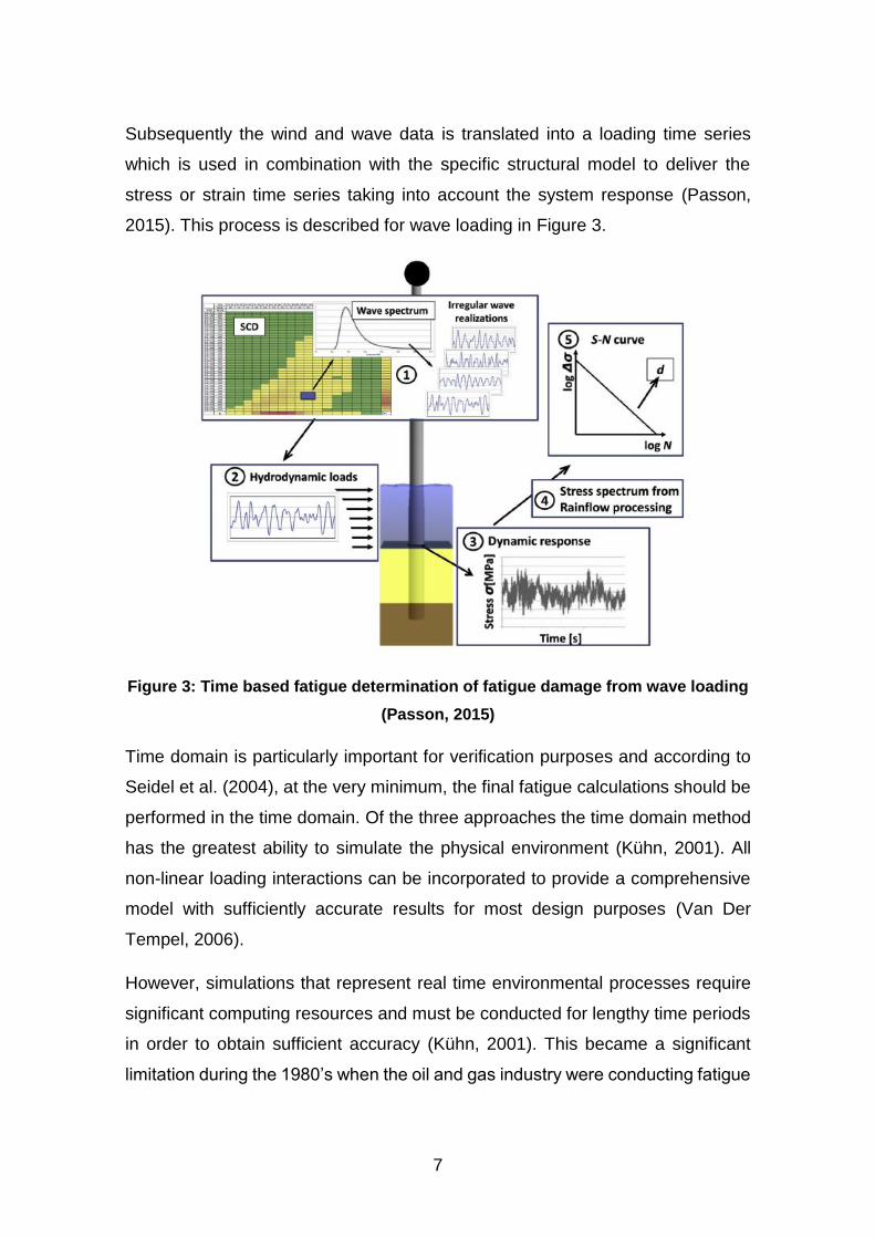
Subsequently the wind and wave data is translated into a loading time series
which is used in combination with the specific structural model to deliver the
stress or strain time series taking into account the system response (Passon,
2015). This process is described for wave loading in Figure 3.
Figure 3: Time based fatigue determination of fatigue damage from wave loading
(Passon, 2015)
Time domain is particularly important for verification purposes and according to
Seidel et al. (2004), at the very minimum, the final fatigue calculations should be
performed in the time domain. Of the three approaches the time domain method
has the greatest ability to simulate the physical environment (Kühn, 2001). All
non-linear loading interactions can be incorporated to provide a comprehensive
model with sufficiently accurate results for most design purposes (Van Der
Tempel, 2006).
However, simulations that represent real time environmental processes require
significant computing resources and must be conducted for lengthy time periods
in order to obtain sufficient accuracy (Kühn, 2001). This became a significant
limitation during the 1980’s when the oil and gas industry were conducting fatigue
8
analyses of oil platforms subjected to in excess of 70 load combinations acting
on the structure at any moment in time (Halfpenny, 1999).
Currently the offshore industry standard for fatigue analyses are for calculations
to be conducted in the frequency domain (Van Der Tempel, 2006) and the only
offshore fatigue calculations conducted in the time domain are for systems
demonstrating significant non-linearity, such as floating structures (Kühn, 2001).
1.2.4 Frequency Domain
Frequency domain analysis also known as spectral analysis for fatigue
calculations, is an extremely powerful method for establishing the structural
response of linearly excited offshore systems (Seidel, 2014). Frequency domain
fatigue calculations increased significantly during the 1980’s and early 1990’s as
a method to mitigate a lack of computational resources required to perform
fatigue calculations in the time domain (Van Der Tempel, 2006). Structures
subject to dynamic loading from wind and waves are well suited to spectral fatigue
analysis due to:
a) The statistically stationary assumptions made for wind speeds and wave
amplitudes.
b) The ability to consider both wind and wave loading regimes independent during
the calculation process (Barltrop and Adams, 1991).
According to the offshore standard Det Norske Veritas (2014), wind speeds are
considered stationary over any given ten minute period with constant mean and
standard deviation, while for waves the stationary duration is assumed to last for
three hours (Det Norske Veritas, 2014). These assumptions permit the
independent calculation of the wind and wave spectra and the subsequent
separate calculation of the structural loading from these two sources of structural
excitation (Det Norske Veritas, 2014). Furthermore, offshore wind turbines with
monopile foundations experience a mudline bending stress that is linearly
proportional to both the wind speed and wave amplitude. Thus from the wind and
wave spectra two separate mudline bending stress spectra can be established in
a relatively straightforward fashion (Barltrop and Adams, 1991). The final process
9
is the superposition of the system response from wind and wave loading to
establish the accumulative fatigue damage. Various approaches can be adopted
for these final stages and will be discussed and explored in greater detail in the
coming chapters.
Both the time and frequency domain approaches for fatigue analysis provide
equally acceptable methods for offshore wind turbines with monopile foundations
and are also entirely interchangeable via the Fourier transform (Van Der Tempel,
2006). Every signal can be described as values changing in time or by the
combination of the fundamental frequencies (Stein, 2000). By performing a
Fourier transformation the random time signal can be described by the sum of
numerous sine waves each with their own frequency, amplitude and phase thus
moving from the time to the frequency domain (Van Der Tempel, 2006). Equally
the inverse procedure can be performed to revert back to the time domain.
The spectral approach becomes limited for systems experiencing non-linearities
in the structure’s loading regime. For an offshore wind turbine system this occurs
from wave drag which is calculated using the Morison equation (section 2.3.6).
However, the literature states that for slender monopile foundations the wave
resistance is dominated by inertia, resulting in the ability to neglect the drag term
in the Morison equation thus making spectral analysis possible (Seidel, 2014,
Arany et al., 2014, Van Der Tempel, 2006).
Both the time and frequency domain methodologies are well suited to the fatigue
analysis of an offshore wind turbine and monopile structure. While the time
domain represents a specific stochastic process over a specific moment in time,
the frequency domain describes every stochastic possibility (Van Der Tempel,
2006). For the reasons discussed above, the majority of this investigation has
been conducted in the frequency domain to simplify the procedure and to limit
the computational resources required for the analysis. However, towards the end
of the study the inverse Fourier Transform has been applied to generate a
mudline bending stress time history in order to establish the damage equivalent
stress range value via Rainflow Counting and the subsequent fatigue life from the
relevant S-N curve.

10
1.3 Aim and Objectives
The aim of this investigation is to present a numerical model in Matlab capable of
performing an integrated wind and wave fatigue analysis of an offshore wind
turbine and monopile foundation. The model will be used to establish how
different superposition methods of the wind and wave stress spectra effect the
overall fatigue life.
To achieve this aim the following objectives will be addressed:
1. Identify and define the characteristics of a suitable reference wind turbine
system and deployment site
2. Conduct a detailed review of relevant theory in the literature
3. Identify and present a suitable methodology to meet the outlined aim
4. Develop and implement the methodology in a number of Matlab scripts
5. Define and justify all simulation input parameters
6. Run a series of simulations to establish how different wind and wave
superposition methodologies effect the final system fatigue life
7. Discuss the results and the limitations of the approaches used
8. Identify areas for future research

11
2 METHODOLOGY
This chapter describes, in detail, all relevant theory necessary to carry out an
integrated fatigue analysis of an offshore wind turbine and monopile foundation.
The information presented has been obtained from a wide variety of sources
including offshore standards, theoretical text books and peer-reviewed journal
articles. In the proceeding section a methodological overview can be found,
describing the various stages used in the form of a flow chart while additional
supporting material can be found in the appendices at the end of this study.
12
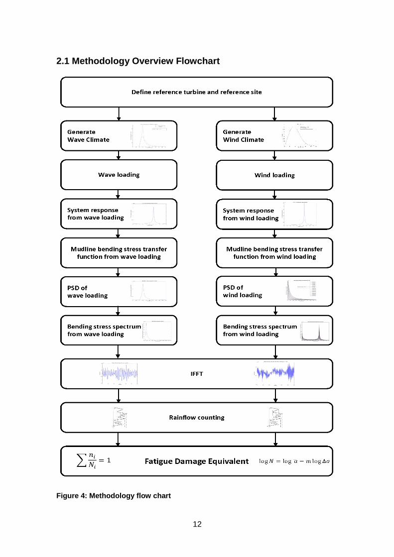
2.1 Methodology Overview Flowchart
Figure 4: Methodology flow chart
13
2.2 Reference Parameters
2.2.1 Reference Site Conditions
To perform a fatigue analysis on an offshore wind turbine and monopile
foundation, it was necessary to define all governing characteristics. This was
undertaken by considering characteristics that typify the current UK offshore wind
turbine installations using available data.
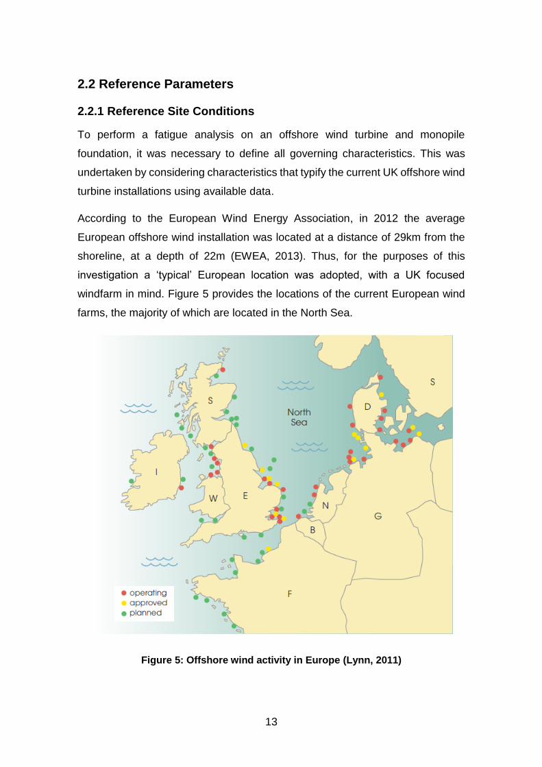
According to the European Wind Energy Association, in 2012 the average
European offshore wind installation was located at a distance of 29km from the
shoreline, at a depth of 22m (EWEA, 2013). Thus, for the purposes of this
investigation a ‘typical’ European location was adopted, with a UK focused
windfarm in mind. Figure 5 provides the locations of the current European wind
farms, the majority of which are located in the North Sea.
Figure 5: Offshore wind activity in Europe (Lynn, 2011)
14
Once the reference site parameters were defined it was important to define the
corresponding sea state parameters, namely the significant wave height (Hs),
and mean zero-crossing period (Tz). A representative significant wave height for
a location roughly 30km from the UK East Coast was found to be approximately
1.5m (see Figure 30 in Appendix A) and a typical corresponding mean zero-
crossing period was chosen of 5 seconds (Van Der Tempel, 2006). Further
description of the significant wave height and mean zero-crossing period can be
found in Table 3. Finally the long-term mean wind speed had to be defined in
order to establish the offshore wind climate at the reference site. This was
assumed to be 10m/s from data presented by Van Der Tempel (2006) (see Figure
35 in Appendix G).
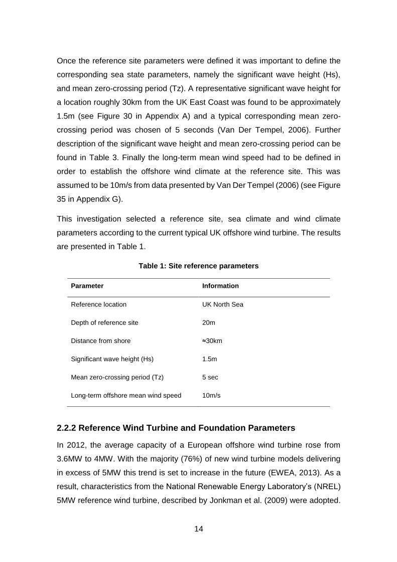
This investigation selected a reference site, sea climate and wind climate
parameters according to the current typical UK offshore wind turbine. The results
are presented in Table 1.
Table 1: Site reference parameters
Parameter Information
Reference location UK North Sea
Depth of reference site 20m
Distance from shore ≈30km
Significant wave height (Hs) 1.5m
Mean zero-crossing period (Tz) 5 sec
Long-term offshore mean wind speed 10m/s
2.2.2 Reference Wind Turbine and Foundation Parameters
In 2012, the average capacity of a European offshore wind turbine rose from
3.6MW to 4MW. With the majority (76%) of new wind turbine models delivering
in excess of 5MW this trend is set to increase in the future (EWEA, 2013). As a
result, characteristics from the National Renewable Energy Laboratory’s (NREL)
5MW reference wind turbine, described by Jonkman et al. (2009) were adopted.
15
Despite the very comprehensive description given by Jonkman et al. (2009), for
the NREL turbine, there is a lack of information pertaining to the offshore
monopile foundation. Thus, a number of assumptions were necessarily made to
provide the foundation parameters.
According to Jonkman et al. (2009) the NREL reference turbine has a hub height
of 90m with a tower top diameter of 3.87 m and a thickness of 0.019 m. The tower
itself is 87.6m high meaning that the hub is at a height of 2.4m above the tower
top. The tower base diameter is 6m with a thickness of 0.027m. The resulting
masses for the hub, nacelle and tower are given in Table 2.
It was assumed that the foundation height was equal to the mean water depth
(20m), and by making an assumption regarding the foundation diameter,
thickness and material density, the foundation mass can be estimated. According
to Busby (2012) and Musial (2011), the diameter of a modern monopile
foundation is currently around 6m. The reference diameter for this investigation
was therefore assumed have a uniform diameter across its height and equal to
the tower base diameter of 6m. A monopile foundation with a 6m diameter,
according to Margariti et al. (2015), can have a wall thickness up to 0.15m. This
was therefore selected as the foundation reference thickness.
Finally, the NREL reference turbine (Jonkman et al., 2009) quotes the density of
the tower steel as 8500kg/m3 rather than the typical value of 7850kg/m3 to
account for the paint, bolts, welds and flanges. The density of the foundation steel
is assumed equal to the density of the tower steel. Taking all the above
parameters into account the foundation reference mass was found (see Table 2).
This investigation has been conducted without taking into consideration the
effects of a transition piece between the tower and foundation, the effects of
which are beyond the scope of this project. Thus for the purposes of this study
the base of the tower sits on top of the top of the foundation, both of which have
equal diameters.

16
Table 2: Turbine and foundation reference parameters
Component Mass [kg]
Hub 56780
Nacelle 240000
Tower 347460
Foundation 237328
TOTAL 881568
Finally, the turbine operational wind speeds must also be defined for the
calculation of the turbine thrust. For the 5MW NREL reference turbine the cut in
speed is quoted as 3m/s and the cut out speed is quoted at 25m/s.
17
2.3 Wave Loading
In this section the procedure for establishing the wave loading on a monopile
foundation is established.
2.3.1 Wave Climate
Wave processes are random in nature consisting of irregular wave shapes,
heights, lengths and propagation speeds. Thus, in order to model wave
processes, a random mathematical model is recommended (Det Norske Veritas,
2010). To empirically establish the sea state at a site of interest the most
important data to collect includes the wave maximum and minimum height, the
strange peaks and the slow variations (Van Der Tempel, 2006). This data must
be collected over long periods of time, ideally for more than ten years (Det Norske
Veritas, 2014). Wave data can be collected from a number of sources including:
Satellite data
Visual measurements
Wave buoys
(Tupper, 1996).
As previously mentioned, sea states are considered stationary random processes
with a stationery period of three hours. However, in reality this can vary from
around 30 minutes and up to 10 hours (Det Norske Veritas, 2010).
In the absence of empirically collected specific sea state data, general long term
wave statistics can be used to describe a sea state with the help of a wave
spectrum (Det Norske Veritas, 2014). A description of the basic wave parameters
is provided in Table 3.
18
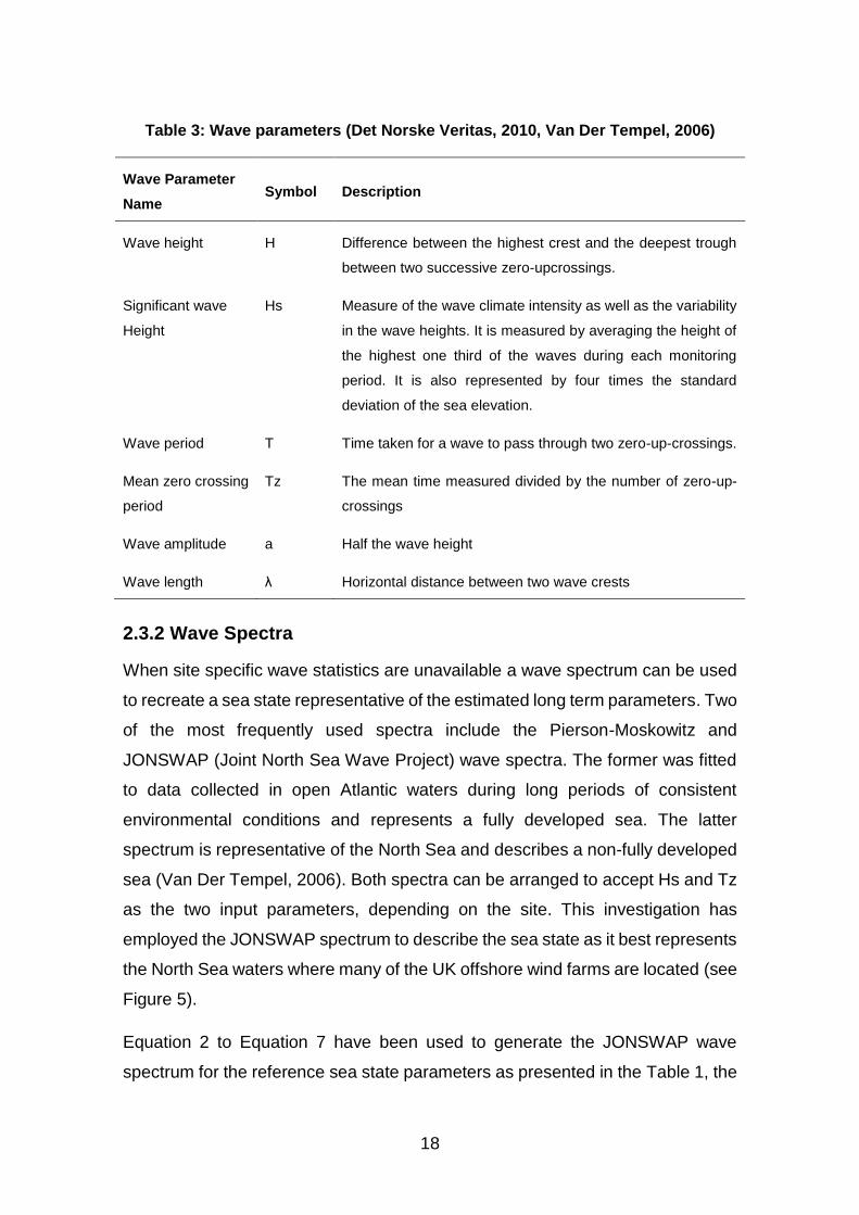
Table 3: Wave parameters (Det Norske Veritas, 2010, Van Der Tempel, 2006)
Wave Parameter
Name Symbol Description
Wave height H Difference between the highest crest and the deepest trough
between two successive zero-upcrossings.
Significant wave
Height
Hs Measure of the wave climate intensity as well as the variability
in the wave heights. It is measured by averaging the height of
the highest one third of the waves during each monitoring
period. It is also represented by four times the standard
deviation of the sea elevation.
Wave period T Time taken for a wave to pass through two zero-up-crossings.
Mean zero crossing
period
Tz The mean time measured divided by the number of zero-up-
crossings
Wave amplitude a Half the wave height
Wave length λ Horizontal distance between two wave crests
2.3.2 Wave Spectra
When site specific wave statistics are unavailable a wave spectrum can be used
to recreate a sea state representative of the estimated long term parameters. Two
of the most frequently used spectra include the Pierson-Moskowitz and
JONSWAP (Joint North Sea Wave Project) wave spectra. The former was fitted
to data collected in open Atlantic waters during long periods of consistent
environmental conditions and represents a fully developed sea. The latter
spectrum is representative of the North Sea and describes a non-fully developed
sea (Van Der Tempel, 2006). Both spectra can be arranged to accept Hs and Tz
as the two input parameters, depending on the site. This investigation has
employed the JONSWAP spectrum to describe the sea state as it best represents
the North Sea waters where many of the UK offshore wind farms are located (see
Figure 5).
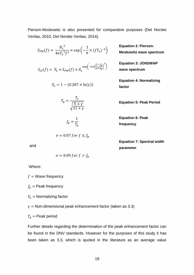
Equation 2 to Equation 7 have been used to generate the JONSWAP wave
spectrum for the reference sea state parameters as presented in the Table 1, the
19
Pierson-Moskowitz is also presented for comparative purposes (Det Norske
Veritas, 2010, Det Norske Veritas, 2014).
𝑆𝑃𝑀(𝑓) = 𝐻𝑠
2
4𝜋𝑇𝑧4𝑓5
× exp (−1
𝜋× (𝑓𝑇𝑧)−4)
Equation 2: Pierson-
Moskowitz wave spectrum
𝑆𝐽𝑆(𝑓) = 𝐹𝑛 × 𝑆𝑃𝑀(𝑓) × 𝐹𝑛
exp(−0.5(𝑓−𝑓𝑝
𝜎×𝑓𝑝)
2
)
Equation 3: JONSWAP
wave spectrum
𝐹𝑛 = 1 − (0.287 × ln(𝛾)) Equation 4: Normalizing
factor
𝑇𝑝 =𝑇𝑧
√5 + 𝛾
11 + 𝛾
Equation 5: Peak Period
𝑓𝑝 =1
𝑇𝑝
Equation 6: Peak
frequency
𝜎 = 0.07 𝑓𝑜𝑟 𝑓 ≤ 𝑓𝑝
and
𝜎 = 0.09 𝑓𝑜𝑟 𝑓 > 𝑓𝑝
Equation 7: Spectral width
parameter
Where:
𝑓 = Wave frequency
𝑓𝑝 = Peak frequency
𝐹𝑛 = Normalizing factor
𝛾 = Non-dimensional peak enhancement factor (taken as 3.3)
𝑇𝑝 = Peak period
Further details regarding the determination of the peak enhancement factor can
be found in the DNV standards. However for the purposes of this study it has
been taken as 3.3, which is quoted in the literature as an average value

20
representative of not fully developed seas such as those found in the North Sea
(Det Norske Veritas, 2014, Van Der Tempel, 2006, Patel, 1989, Veldkamp and
Van Der Tempel, 2005, Chakrabarti, 2005).
Figure 6 demonstrates the two wave spectra for the case when Hs=1.5m, Tz=5
seconds and γ=3.3.
Figure 6: Wave spectra
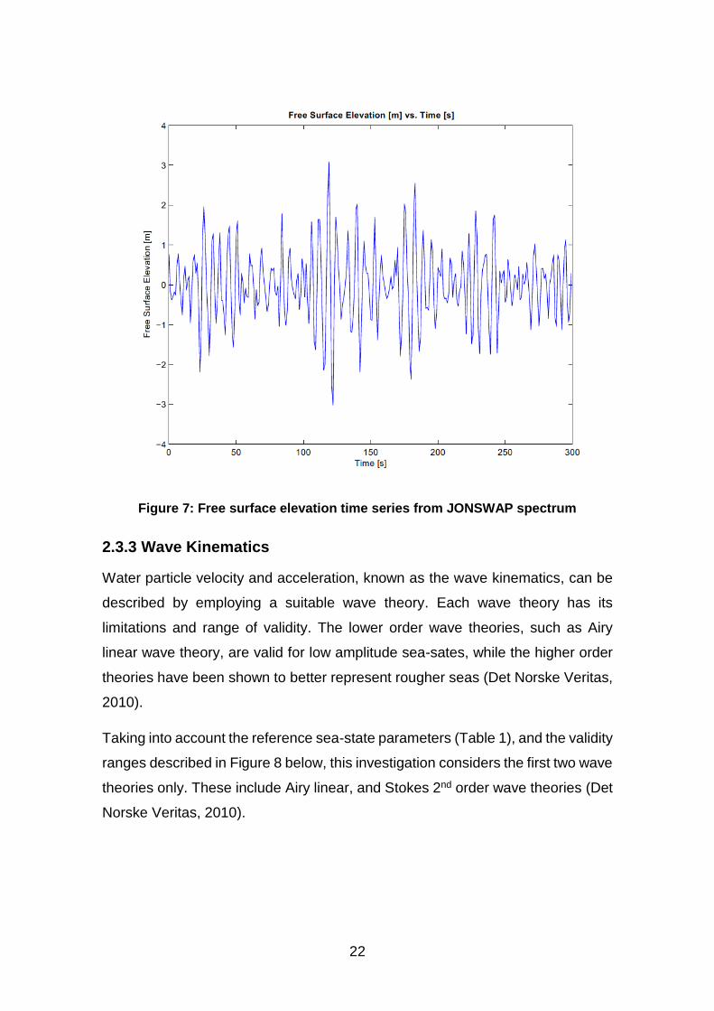
From a wave spectrum, it is possible to generate a time series of wave elevation
by distilling the random wave amplitudes into regular wave characteristics (Patel,
1989). A phase angle between 0 and 2π is randomly assigned to each wave. The
sum of all the waves for a given frequency and at a given moment in time provide
the sea surface elevation (Van Der Tempel, 2006). Equation 8 and Equation 9
describes how this process is carried out numerically while Figure 7 presents an
example time series generated from the JONSWAP spectrum described above.
For further information refer to Patel (1989).
21
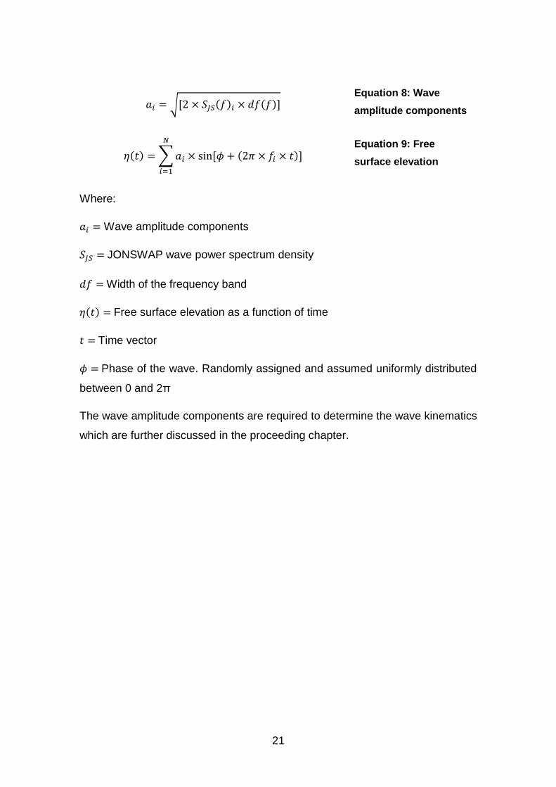
𝑎𝑖 = √[2 × 𝑆𝐽𝑆(𝑓)𝑖 × 𝑑𝑓(𝑓)] Equation 8: Wave
amplitude components
𝜂(𝑡) = ∑ 𝑎𝑖
𝑁
𝑖=1
× sin [𝜙 + (2𝜋 × 𝑓𝑖 × 𝑡)] Equation 9: Free
surface elevation
Where:
𝑎𝑖 = Wave amplitude components
𝑆𝐽𝑆 = JONSWAP wave power spectrum density
𝑑𝑓 = Width of the frequency band
𝜂(𝑡) = Free surface elevation as a function of time
𝑡 = Time vector
𝜙 = Phase of the wave. Randomly assigned and assumed uniformly distributed
between 0 and 2π
The wave amplitude components are required to determine the wave kinematics
which are further discussed in the proceeding chapter.
22
Figure 7: Free surface elevation time series from JONSWAP spectrum
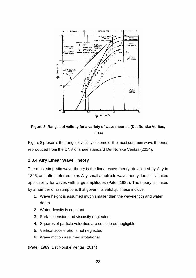
2.3.3 Wave Kinematics
Water particle velocity and acceleration, known as the wave kinematics, can be
described by employing a suitable wave theory. Each wave theory has its
limitations and range of validity. The lower order wave theories, such as Airy
linear wave theory, are valid for low amplitude sea-sates, while the higher order
theories have been shown to better represent rougher seas (Det Norske Veritas,
2010).
Taking into account the reference sea-state parameters (Table 1), and the validity
ranges described in Figure 8 below, this investigation considers the first two wave
theories only. These include Airy linear, and Stokes 2nd order wave theories (Det
Norske Veritas, 2010).
23
Figure 8: Ranges of validity for a variety of wave theories (Det Norske Veritas,
2014)
Figure 8 presents the range of validity of some of the most common wave theories
reproduced from the DNV offshore standard Det Norske Veritas (2014).
2.3.4 Airy Linear Wave Theory
The most simplistic wave theory is the linear wave theory, developed by Airy in
1845, and often referred to as Airy small amplitude wave theory due to its limited
applicability for waves with large amplitudes (Patel, 1989). The theory is limited
by a number of assumptions that govern its validity. These include:
1. Wave height is assumed much smaller than the wavelength and water
depth
2. Water density is constant
3. Surface tension and viscosity neglected
4. Squares of particle velocities are considered negligible
5. Vertical accelerations not neglected
6. Wave motion assumed irrotational
(Patel, 1989, Det Norske Veritas, 2014)
24
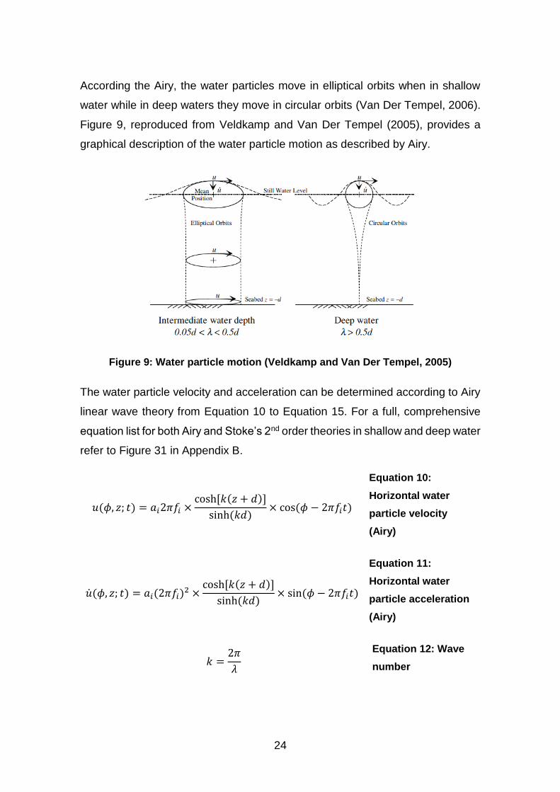
According the Airy, the water particles move in elliptical orbits when in shallow
water while in deep waters they move in circular orbits (Van Der Tempel, 2006).
Figure 9, reproduced from Veldkamp and Van Der Tempel (2005), provides a
graphical description of the water particle motion as described by Airy.
Figure 9: Water particle motion (Veldkamp and Van Der Tempel, 2005)
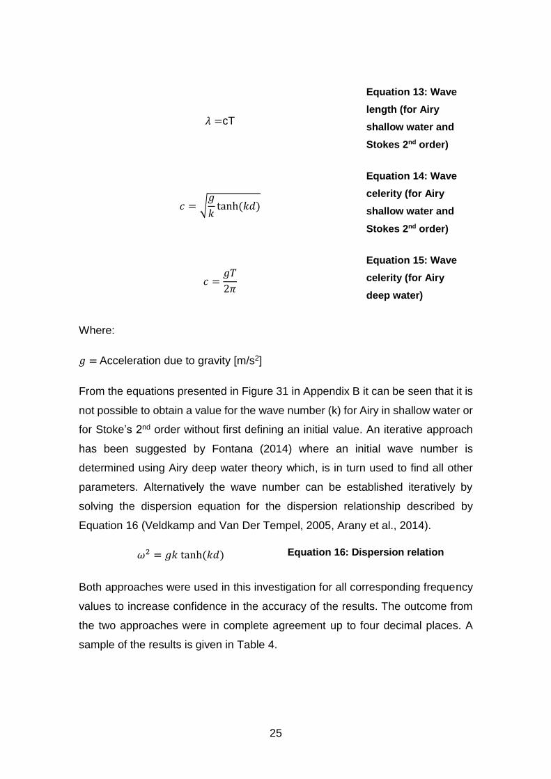
The water particle velocity and acceleration can be determined according to Airy
linear wave theory from Equation 10 to Equation 15. For a full, comprehensive
equation list for both Airy and Stoke’s 2nd order theories in shallow and deep water
refer to Figure 31 in Appendix B.
𝑢(𝜙, 𝑧; 𝑡) = 𝑎𝑖2𝜋𝑓𝑖 ×cosh [𝑘(𝑧 + 𝑑)]
sinh (𝑘𝑑)× cos (𝜙 − 2𝜋𝑓𝑖𝑡)
Equation 10:
Horizontal water
particle velocity
(Airy)
�̇�(𝜙, 𝑧; 𝑡) = 𝑎𝑖(2𝜋𝑓𝑖)2 ×
cosh [𝑘(𝑧 + 𝑑)]
sinh (𝑘𝑑)× sin (𝜙 − 2𝜋𝑓𝑖𝑡)
Equation 11:
Horizontal water
particle acceleration
(Airy)
𝑘 =2𝜋
𝜆
Equation 12: Wave
number
25
𝜆 =cT
Equation 13: Wave
length (for Airy
shallow water and
Stokes 2nd order)
𝑐 = √𝑔
𝑘tanh (𝑘𝑑)
Equation 14: Wave
celerity (for Airy
shallow water and
Stokes 2nd order)
𝑐 =𝑔𝑇
2𝜋
Equation 15: Wave
celerity (for Airy
deep water)
Where:
𝑔 = Acceleration due to gravity [m/s2]
From the equations presented in Figure 31 in Appendix B it can be seen that it is
not possible to obtain a value for the wave number (k) for Airy in shallow water or
for Stoke’s 2nd order without first defining an initial value. An iterative approach
has been suggested by Fontana (2014) where an initial wave number is
determined using Airy deep water theory which, is in turn used to find all other
parameters. Alternatively the wave number can be established iteratively by
solving the dispersion equation for the dispersion relationship described by
Equation 16 (Veldkamp and Van Der Tempel, 2005, Arany et al., 2014).
𝜔2 = 𝑔𝑘 tanh (𝑘𝑑) Equation 16: Dispersion relation
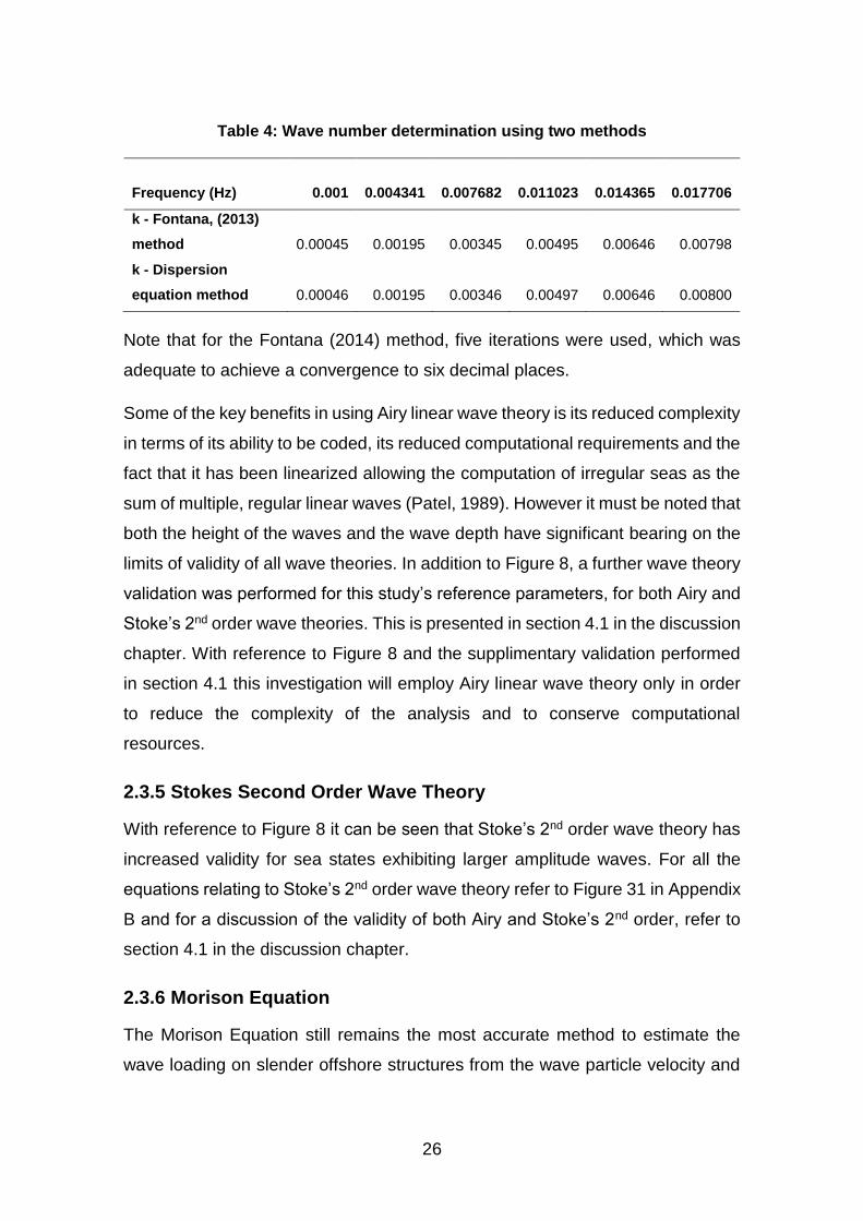
Both approaches were used in this investigation for all corresponding frequency
values to increase confidence in the accuracy of the results. The outcome from
the two approaches were in complete agreement up to four decimal places. A
sample of the results is given in Table 4.
26
Table 4: Wave number determination using two methods
Frequency (Hz) 0.001 0.004341 0.007682 0.011023 0.014365 0.017706
k - Fontana, (2013)
method 0.00045 0.00195 0.00345 0.00495 0.00646 0.00798
k - Dispersion
equation method 0.00046 0.00195 0.00346 0.00497 0.00646 0.00800
Note that for the Fontana (2014) method, five iterations were used, which was
adequate to achieve a convergence to six decimal places.
Some of the key benefits in using Airy linear wave theory is its reduced complexity
in terms of its ability to be coded, its reduced computational requirements and the
fact that it has been linearized allowing the computation of irregular seas as the
sum of multiple, regular linear waves (Patel, 1989). However it must be noted that
both the height of the waves and the wave depth have significant bearing on the
limits of validity of all wave theories. In addition to Figure 8, a further wave theory
validation was performed for this study’s reference parameters, for both Airy and
Stoke’s 2nd order wave theories. This is presented in section 4.1 in the discussion
chapter. With reference to Figure 8 and the supplimentary validation performed
in section 4.1 this investigation will employ Airy linear wave theory only in order
to reduce the complexity of the analysis and to conserve computational
resources.
2.3.5 Stokes Second Order Wave Theory
With reference to Figure 8 it can be seen that Stoke’s 2nd order wave theory has
increased validity for sea states exhibiting larger amplitude waves. For all the
equations relating to Stoke’s 2nd order wave theory refer to Figure 31 in Appendix
B and for a discussion of the validity of both Airy and Stoke’s 2nd order, refer to
section 4.1 in the discussion chapter.
2.3.6 Morison Equation
The Morison Equation still remains the most accurate method to estimate the
wave loading on slender offshore structures from the wave particle velocity and
27
acceleration (Veldkamp and Van Der Tempel, 2005). Structural members which
have a diameter divided by the wavelength less than 0.2 can be considered
slender and are assumed not to interact or influence the wave properties (Patel,
1989). Thus, the total wave forces on slender members are given as the sum of
the inertia forces (due to fluid acceleration) and drag forces (due to the fluid
velocity) (Patel, 1989). For the purposes of this investigation, the monopile
structure is considered slender. If this assumption no longer holds true, the model
will no longer be valid without additional modification to take diffraction into
account.
The forces exerted on the slender monopile structure can then be represented
by the Morison equation which includes the integration of the water particle
velocity and acceleration over the depth (Patel, 1989). The first term in the
equation represents the inertia force and the second term represents the drag
force.
𝐹 = 𝐶𝑀𝜌𝜋𝑟2 ∫ �̇�0
−𝑑
𝑑𝑧 + 𝐶𝐷𝜌𝜋𝑟 ∫ |𝑢|0
−𝑑
𝑢 𝑑𝑧 Equation 17: Morison
Equation
Where:
𝐹 = Total wave force on the member found by integration over the water depth
𝐶𝑀 = Inertia coefficient
𝐶𝐷 = Drag coefficient
𝜌 = Fluid density
𝑟 = Member radius
�̇� = Water particle acceleration
|𝑢|𝑢 = Water particle |velocity| * velocity
A limitation of using the Morison equation is that it requires the selection of two
empirical parameters for the load calculation: the drag and inertia coefficients.
The selection of the drag and inertia coefficients are dependent on empirical data
28
and should be determined experimentally. The DNV standards suggest various
methods to determine suitable drag and inertia coefficients for design purposes,
however for an offshore monopile foundation the literature suggests suitable
values. This investigation has taken values recommended in the literature
relevant to offshore wind turbines with monopile foundations. Thus, the drag
coefficient has been taken as 0.70 assuming a smooth monopile (no marine
growth present), and 2.0 as the inertia coefficient (Van Der Tempel, 2006,
Veldkamp and Van Der Tempel, 2005, Barltrop and Adams, 1991).
The full and detailed integration process, including the final integrated equations
are given in Appendix C for Airy and Appendix D for Stoke’s 2nd order.
29
2.4 Wind Loading
In this section the procedure for establishing the wind loading on a monopile
foundation is established.
2.4.1 Wind Climate
As well as varying with time, wind speed varies with height due to wind shear.
Typically, the wind reference height is taken as 10m and wind speed average
times vary between 1, 10 and 60 minutes (Det Norske Veritas, 2010). Wind shear
occurs in approximately the first 2km of the atmosphere and is a result of friction
with the ground where the wind speed is zero (Van Der Tempel, 2006). To take
this into consideration, models have been developed which depend on the
surface roughness (topography) and the reference height.
The wind climate of a site can be separated into two categories: normal wind
climate and extreme wind climate. The former is used as the foundation for
fatigue load calculations and as such will be the focus of this investigation (Det
Norske Veritas, 2014). Normal wind conditions are described by air density, a
long term distribution of the 10 minute wind speed and the wind shear and
turbulence. Both are dependent on height and terrain (Det Norske Veritas, 2014,
Van Der Tempel, 2006).
2.4.2 Normal Wind Conditions
The parameters required to describe the normal wind climate are outlined in Det
Norske Veritas (2014) and include the 10 minute mean wind speed (U10) and the
standard deviation (σ10), during which, constant conditions are assumed. The
intensity in the turbulence during the ten minute period is given as the ratio
between σ10 and U10. Similar to the wave climate, the wind climate can be
described by a wind spectrum as a function of σ10 and U10 some of which are
discussed in the next section.
30
2.4.3 Wind Modelling
To establish the thrust force from the turbine the wind speed must be modelled
which can subsequently be used in combination with the actuator disk theory.
These processes are discussed in the following sections.
2.4.3.1 Actuator Disk Theory
The purpose of a wind turbine is to translate the kinetic energy of the wind into
rotational energy to drive a turbine. The quantity of energy extractable is
governed by the Betz limit determined at 59% (Lynn, 2011). This theoretical limit
is based on linear momentum theory where the mass flow rate in must be equal
to the mass flow rate out. Any decrease in velocity must therefore result in an
increase in volume. This process can be represented using a stream tube (see
Figure 10).
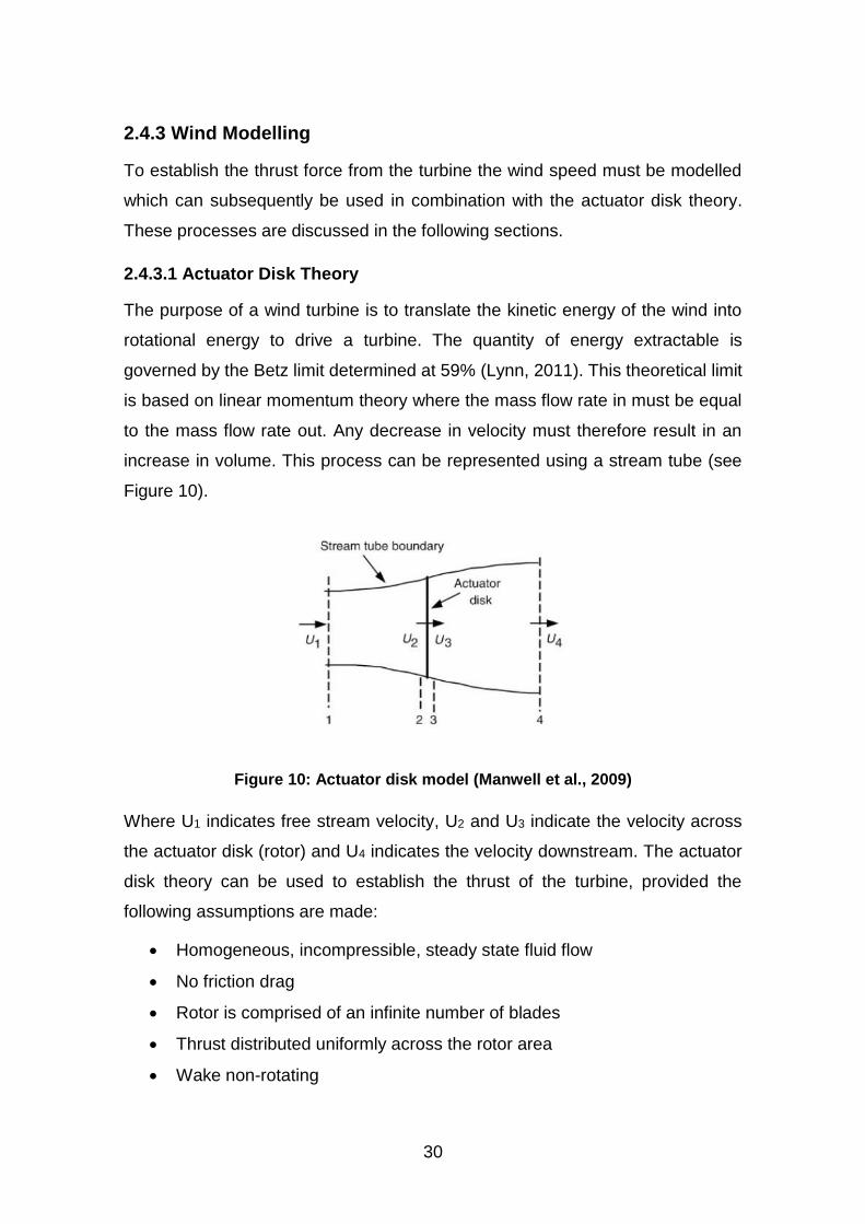
Figure 10: Actuator disk model (Manwell et al., 2009)
Where U1 indicates free stream velocity, U2 and U3 indicate the velocity across
the actuator disk (rotor) and U4 indicates the velocity downstream. The actuator
disk theory can be used to establish the thrust of the turbine, provided the
following assumptions are made:
Homogeneous, incompressible, steady state fluid flow
No friction drag
Rotor is comprised of an infinite number of blades
Thrust distributed uniformly across the rotor area
Wake non-rotating
31
Static pressure far upstream and far downstream is equal to ambient
static pressure
(Manwell et al., 2009)
Employing the conservation of linear momentum and the Bernoulli function for
the two control volumes, an expression for the turbine thrust can be derived (see
(Manwell et al., 2009) or (Lynn, 2011) for derivation).
𝑇 =1
2𝜌𝑎𝐴𝑟𝑜𝑡𝑜𝑟𝑈2[4𝑎(1 − 𝑎)] Equation 18: Thrust - Wind turbine
𝑎 =𝑈1 − 𝑈2
𝑈1
Equation 19: Axial induction factor
Where:
𝑇 = Turbine thrust
𝜌𝑎 = Density of air
𝐴𝑟𝑜𝑡𝑜𝑟 = Rotor area
𝑈 = 𝑈1 = Freestream velocity
𝑈2 = Velocity across the actuator disk
𝑎 = Axial induction factor
From Equation 18 and Equation 19 it can be seen that to establish the thrust from
the free stream velocity it is necessary to know the flow velocity across the disk
(𝑈2). For the current investigation 𝑈2 is not known therefore an alternative method
has been used to establish the axial induction factor (𝑎).
Two methods can be used to find the axial induction factor, the first uses Blade
Element Momentum theory (BEM theory), and the second uses the equation for
the thrust coefficient. Both methods can be used to estimate the turbine thrust
from the instantaneous wind speed (Van Der Tempel, 2006, Arany et al., 2014).
Although BEM theory is more accurate, it also requires highly detailed information
pertaining to the turbine blade geometry which is often difficult to obtain. Such a
32
detailed analysis is not necessary for the purpose of this investigation. Therefore,
to estimate the axial induction factor the latter method was used, and to estimate
the thrust coefficient, Frohboese et al. (2010)’s thrust coefficient estimation
method has been used (see Section 2.7.2). Appendix E presents the process
used to find the axial induction factor.
Once the axial induction factor has been established the actuator disk theory can
be used directly with the free stream wind velocity to determine the turbine thrust.
2.4.3.2 Wind Speed Distributions
Probability density functions (pdf’s) allow the probability of occurrence of a given
wind speed within a given range to be established (Lynn, 2011). Two of the most
common probability distributions used in wind modelling are the Rayleigh and
Weibull probability distributions. The Rayleigh distribution requires knowledge of
one parameter: the mean wind speed, while the Weibull distribution requires the
determination of two parameters: a shape factor (k) and a scale factor (c). Both
‘k’ and ‘c’ are functions of the mean wind speed and the standard deviation
(Manwell et al., 2009). The Weibull distribution is preferred when additional data
is available and it has also been shown to represent a broader range of wind
climates (Lynn, 2011). Thus the Weibull distribution has been used to model the
wind climate in this investigation, and the procedure employed is presented in
Appendix G.
Assuming a long term mean wind speed of 10m/s (Table 1), and by following the
methodologies outlined in Appendix G, the number of occurrences for each mean
wind speed from 0.5m/s up to 30m/s, over the course of one year were found
(Figure 11).
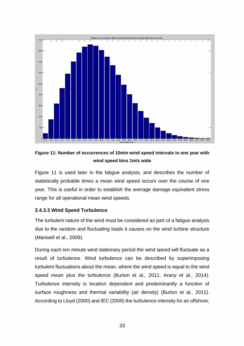
33
Figure 11: Number of occurrences of 10min wind speed intervals in one year with
wind speed bins 1m/s wide
Figure 11 is used later in the fatigue analysis, and describes the number of
statistically probable times a mean wind speed occurs over the course of one
year. This is useful in order to establish the average damage equivalent stress
range for all operational mean wind speeds.
2.4.3.3 Wind Speed Turbulence
The turbulent nature of the wind must be considered as part of a fatigue analysis
due to the random and fluctuating loads it causes on the wind turbine structure
(Manwell et al., 2009).
During each ten minute wind stationary period the wind speed will fluctuate as a
result of turbulence. Wind turbulence can be described by superimposing
turbulent fluctuations about the mean, where the wind speed is equal to the wind
speed mean plus the turbulence (Burton et al., 2011, Arany et al., 2014).
Turbulence intensity is location dependent and predominantly a function of
surface roughness and thermal variability (air density) (Burton et al., 2011).
According to Lloyd (2000) and IEC (2009) the turbulence intensity for an offshore,
34
near shore site, representative of the UK North Sea wind turbine locations, is
approximately 12% for wind speeds above 5m/s (see Figure 32 and Figure 33).
For the purposes of this investigation the turbulence intensity has been assumed
to be constant for all operational ten minute mean wind speeds at 12%. The
relationship between the turbulence intensity and mean wind speed standard
deviation is described by Equation 20.
𝐼 =𝜎
�̅�10
Equation 20: Turbulence Intensity
Where:
𝐼 = Turbulence intensity
�̅�10 = Ten minute mean wind speed
𝜎 = Ten minute wind speed standard deviation
The turbulence in the wind during any given ten minute period can be described
by a wind turbulence power spectral density (PSD), provided the ten minute mean
wind speed and standard deviation are known. Wind turbulence PSD’s describe
the frequency content of wind speed variations. Two of the most commonly used
spectra are the Karman and Kaimal spectra (Burton et al., 2011, Van Der Tempel,
2006). While the Karman spectra has been cited as a good representation of
turbulence in wind tunnels, the Kaimal spectrum is said to better describe
atmospheric turbulence observations (Burton et al., 2011). With reference to the
above, this investigation employs the Kaimal spectrum. The process used to
generate the Kiamal spectrum for each operational mean wind speed is given in
Appendix H and the results are presented below in Figure 12. Note that the
operational wind speeds for the NREL 5MW reference turbine range from 3m/s
to 25m/. Therefore the mean wind speeds range from 3.5m/s to 24.5m/s to cover
all operational wind conditions.
35
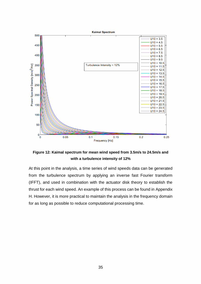
Figure 12: Kaimal spectrum for mean wind speed from 3.5m/s to 24.5m/s and
with a turbulence intensity of 12%
At this point in the analysis, a time series of wind speeds data can be generated
from the turbulence spectrum by applying an inverse fast Fourier transform
(IFFT), and used in combination with the actuator disk theory to establish the
thrust for each wind speed. An example of this process can be found in Appendix
H. However, it is more practical to maintain the analysis in the frequency domain
for as long as possible to reduce computational processing time.
36
2.5 System Response from Wind Loading
The dynamic response of systems subjected to time-varying loads requires
careful consideration (Van Der Tempel, 2006) which is what will be explored in
this section. As previously discussed, when the natural frequency of a system
coincides with the frequencies experienced from the wind and wave loading, an
amplification in the stresses and subsequently the fatigue damage occur (Arany
et al., 2014). This phenomenon can be avoided by determining the dynamic
amplification factor (DAF) which depends on the system damping. To establish
the DAF very specific information is required pertaining the turbine, tower,
foundation and soil conditions. This study has acquired this information based on
the NREL 5MW reference turbine, presented in section 2.2.
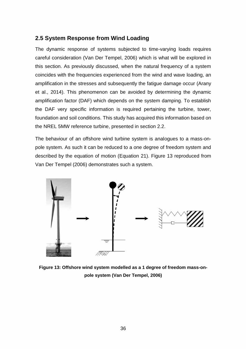
The behaviour of an offshore wind turbine system is analogues to a mass-on-
pole system. As such it can be reduced to a one degree of freedom system and
described by the equation of motion (Equation 21). Figure 13 reproduced from
Van Der Tempel (2006) demonstrates such a system.
Figure 13: Offshore wind system modelled as a 1 degree of freedom mass-on-
pole system (Van Der Tempel, 2006)
37
𝐹(𝑡) = 𝑚�̈� + 𝑐�̇� + 𝑘𝑥 Equation 21: Equation of motion
Where:
𝐹 = Force [N]
𝑚 = Mass [kg]
𝑐 = Damping coefficient [Ns/m]
𝑘 = Stiffness [N/m]
�̈� = Acceleration [m/s2]
�̇� =Velocity [m/s]
𝑥 = Displacement [m]
The frequency response of the system subjected to a force input 𝐹(𝑡) which is
equal to the delta function 𝛿(𝑡) can be found by taking the Fourier transforms of
both sides of the equation of motion (Equation 21). Provided the system stiffness,
damping coefficient and mass are known the transformation will provide a transfer
function of the tower top load to the tower top displacement. For a more detailed
explanation see Bendat and Piersol (1993) and Van Der Tempel (2006).
𝑋(𝑓) =1/𝑘
1 − (𝑓𝑓𝑛
)2
+𝑖2𝜁𝑓
𝑓𝑛
Equation 22: Frequency response
function for displacement
Where:
𝜁 = Damping ratio (Equation 24)
𝑓𝑛 = Undamped natural frequency (Hz)
𝑋 = Displacement [m]
𝑓𝑛 =1
2𝜋√
𝑘
𝑚
Equation 23: Undamped natural
frequency
38
𝜁 =𝑐
2√𝑘𝑚 Equation 24: Damping ratio
𝑐 = 𝑐𝑐𝑟𝑖𝑡𝑖𝑐𝑎𝑙 × 2√𝑘𝑚 Equation 25: Damping coefficient
The system gain can then be found by taking the modulus of Equation 22 giving:
|𝑋(𝑓)| =1/𝑘
√[1 − (𝑓𝑓𝑛
)2
]
2
+ [2𝜁𝑓𝑓𝑛
]2
Equation 26: Frequency response
function for displacement
It is important to note that although the theory presented above is generalised,
the system gain equation (Equation 26) represents the DAF of the offshore
structure (Arany et al., 2014).
2.5.1 Tower Top Displacement Transfer Function
Regrettably, a tower top displacement transfer function is not provided for the
NREL 5MW reference turbine, nor is the required stiffness and damping
coefficient. However, the mass of the tower, rotor and nacelle are given (Table 2)
and from assumptions made about the foundation, the foundation mass was also
established (Table 2).
In order to find the stiffness of the system accurately, one of two methods can be
used. Either an FEA model is constructed, a tower top load applied and the
deflection recorded, or a similar experiment is performed on the actual specific
turbine to measure the tower top deflection under a given load (Van Der Tempel,
2006). Both of these methods are beyond the scope of this investigation,
therefore the stiffness had to be estimated from information found in the literature.
In a study by Yeter et al. (2014), a scaling method was used to determine the
transfer function for the NREL reference turbine which was based on the transfer
function derived by Van Der Tempel (2006) for a 2MW Vestas turbine at Blyth.
Yeter et al. (2014) found that the peak frequency of the tower top displacement
transfer function was equal to 0.633Hz.
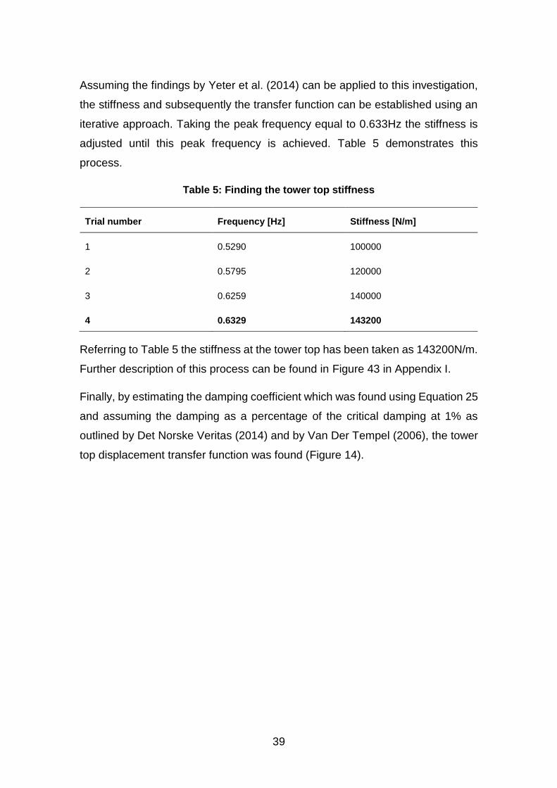
39
Assuming the findings by Yeter et al. (2014) can be applied to this investigation,
the stiffness and subsequently the transfer function can be established using an
iterative approach. Taking the peak frequency equal to 0.633Hz the stiffness is
adjusted until this peak frequency is achieved. Table 5 demonstrates this
process.
Table 5: Finding the tower top stiffness
Trial number Frequency [Hz] Stiffness [N/m]
1 0.5290 100000
2 0.5795 120000
3 0.6259 140000
4 0.6329 143200
Referring to Table 5 the stiffness at the tower top has been taken as 143200N/m.
Further description of this process can be found in Figure 43 in Appendix I.
Finally, by estimating the damping coefficient which was found using Equation 25
and assuming the damping as a percentage of the critical damping at 1% as
outlined by Det Norske Veritas (2014) and by Van Der Tempel (2006), the tower
top displacement transfer function was found (Figure 14).
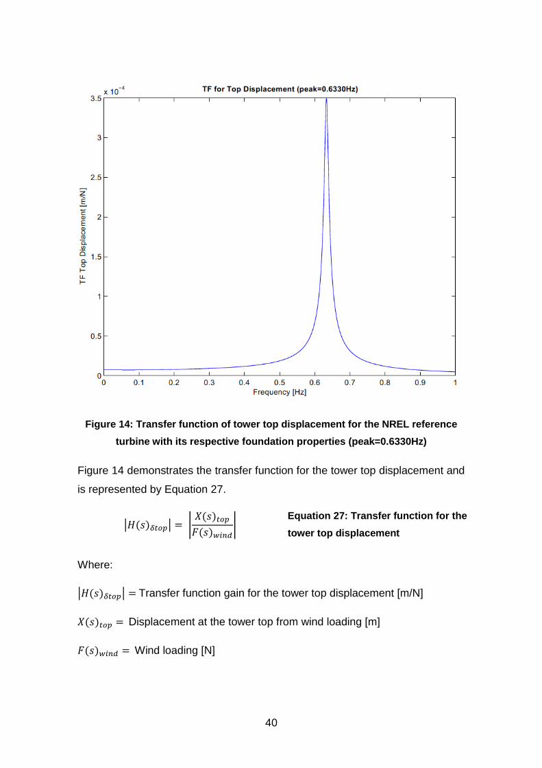
40
Figure 14: Transfer function of tower top displacement for the NREL reference
turbine with its respective foundation properties (peak=0.6330Hz)
Figure 14 demonstrates the transfer function for the tower top displacement and
is represented by Equation 27.
|𝐻(𝑠)𝛿𝑡𝑜𝑝| = |𝑋(𝑠)𝑡𝑜𝑝
𝐹(𝑠)𝑤𝑖𝑛𝑑|
Equation 27: Transfer function for the
tower top displacement
Where:
|𝐻(𝑠)𝛿𝑡𝑜𝑝| = Transfer function gain for the tower top displacement [m/N]
𝑋(𝑠)𝑡𝑜𝑝 = Displacement at the tower top from wind loading [m]
𝐹(𝑠)𝑤𝑖𝑛𝑑 = Wind loading [N]
41
2.6 System Response from Wave Loading
The transfer function required for the wave loading will differ from the tower top
transfer function as a result of the difference in stiffness of the system at the
location of the wave loading. However without precise data of the stiffness along
the length of the turbine the precise transfer function must be found again by
making assumptions and simplifications. This section outlines the methodology
used to establish the transfer function for the mean water level (MWL)
displacement. Three fundamental assumptions must be made before this can be
conducted:
1. The 2nd moment of inertia is constant across the system
2. The transfer function established at the MWL can be applied to the load
data that’s been integrated over the depth
3. The system can be modelled as a linearly elastic beam and follows
Hook’s Law
Assuming all the above, the deflection of the system at the MWL, which was
defined as 20m in section 2.2.1, can be established.
2.6.1 MWL Displacement Transfer Function
To establish the MWL transfer function, the stiffness at the MWL must be
estimated. A detailed description of this process can be found in 0, which found
the MWL stiffness to be 23824900N/m. Finally by following the same process
used to find the tower top displacement transfer function the MWL displacement
transfer function was found (Figure 15).
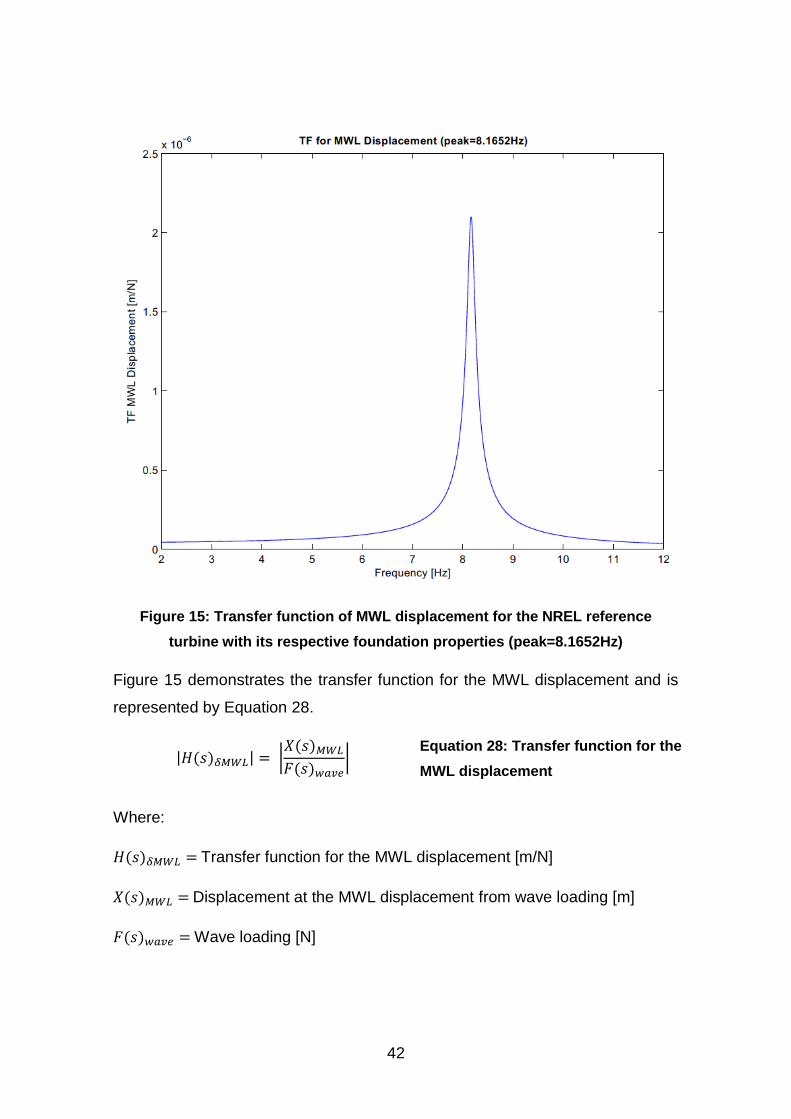
42
Figure 15: Transfer function of MWL displacement for the NREL reference
turbine with its respective foundation properties (peak=8.1652Hz)
Figure 15 demonstrates the transfer function for the MWL displacement and is
represented by Equation 28.
|𝐻(𝑠)𝛿𝑀𝑊𝐿| = |𝑋(𝑠)𝑀𝑊𝐿
𝐹(𝑠)𝑤𝑎𝑣𝑒|
Equation 28: Transfer function for the
MWL displacement
Where:
𝐻(𝑠)𝛿𝑀𝑊𝐿 = Transfer function for the MWL displacement [m/N]
𝑋(𝑠)𝑀𝑊𝐿 = Displacement at the MWL displacement from wave loading [m]
𝐹(𝑠)𝑤𝑎𝑣𝑒 = Wave loading [N]

43
It should be noted that only one transfer function for the wave loading
displacement has been generated at the MWL, therefore a conservative
assumption is made that this transfer function can be employed in conjunction
with the integrated wave load over the depth. The validity of this assumption is
beyond the scope of this investigation and is suggested as an area for future
investigations.
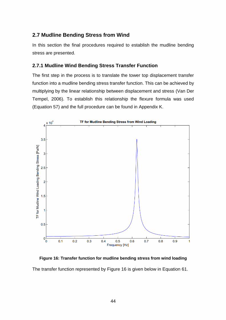
44
2.7 Mudline Bending Stress from Wind
In this section the final procedures required to establish the mudline bending
stress are presented.
2.7.1 Mudline Wind Bending Stress Transfer Function
The first step in the process is to translate the tower top displacement transfer
function into a mudline bending stress transfer function. This can be achieved by
multiplying by the linear relationship between displacement and stress (Van Der
Tempel, 2006). To establish this relationship the flexure formula was used
(Equation 57) and the full procedure can be found in Appendix K.
Figure 16: Transfer function for mudline bending stress from wind loading
The transfer function represented by Figure 16 is given below in Equation 61.
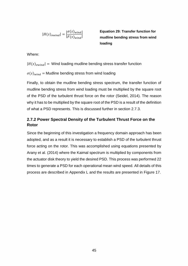
45
|𝐻(𝑠)𝜎𝑤𝑖𝑛𝑑| = |𝜎(𝑠)𝑤𝑖𝑛𝑑
𝐹(𝑠)𝑤𝑖𝑛𝑑|
Equation 29: Transfer function for
mudline bending stress from wind
loading
Where:
|𝐻(𝑠)𝜎𝑤𝑖𝑛𝑑| = Wind loading mudline bending stress transfer function
𝜎(𝑠)𝑤𝑖𝑛𝑑 = Mudline bending stress from wind loading
Finally, to obtain the mudline bending stress spectrum, the transfer function of
mudline bending stress from wind loading must be multiplied by the square root
of the PSD of the turbulent thrust force on the rotor (Seidel, 2014). The reason
why it has to be multiplied by the square root of the PSD is a result of the definition
of what a PSD represents. This is discussed further in section 2.7.3.
2.7.2 Power Spectral Density of the Turbulent Thrust Force on the
Rotor
Since the beginning of this investigation a frequency domain approach has been
adopted, and as a result it is necessary to establish a PSD of the turbulent thrust
force acting on the rotor. This was accomplished using equations presented by
Arany et al. (2014) where the Kaimal spectrum is multiplied by components from
the actuator disk theory to yield the desired PSD. This process was performed 22
times to generate a PSD for each operational mean wind speed. All details of this
process are described in Appendix L and the results are presented in Figure 17.
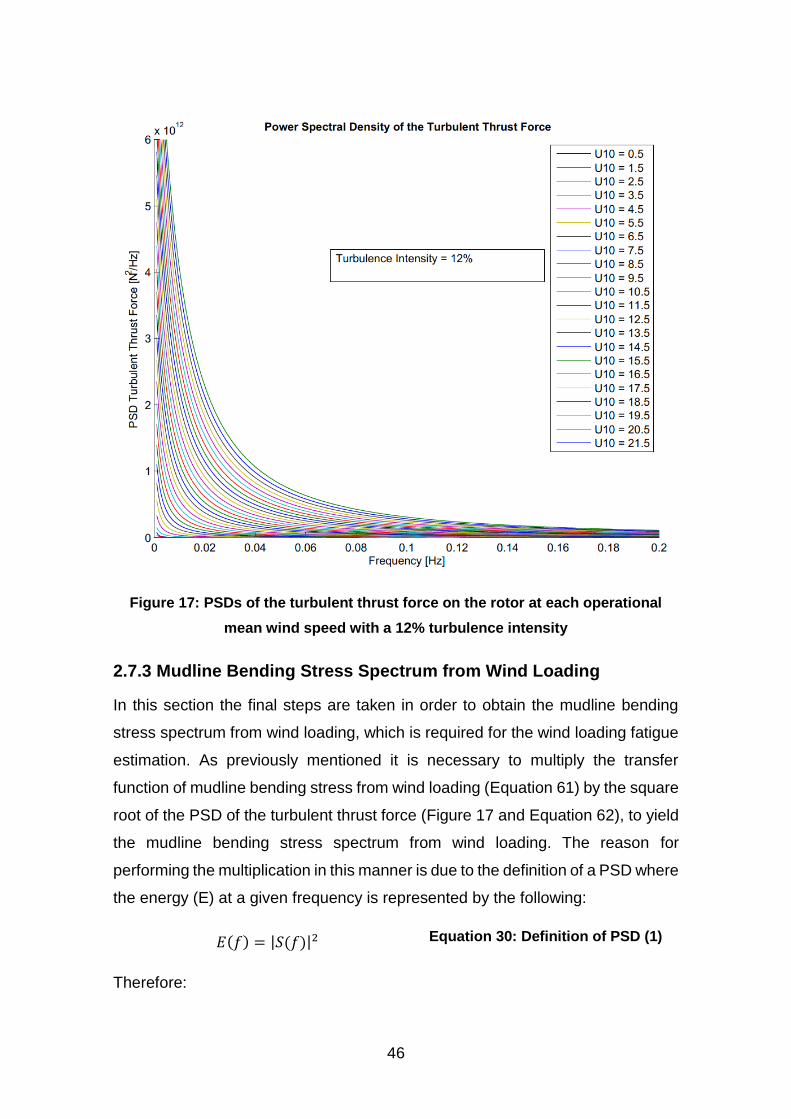
46
Figure 17: PSDs of the turbulent thrust force on the rotor at each operational
mean wind speed with a 12% turbulence intensity
2.7.3 Mudline Bending Stress Spectrum from Wind Loading
In this section the final steps are taken in order to obtain the mudline bending
stress spectrum from wind loading, which is required for the wind loading fatigue
estimation. As previously mentioned it is necessary to multiply the transfer
function of mudline bending stress from wind loading (Equation 61) by the square
root of the PSD of the turbulent thrust force (Figure 17 and Equation 62), to yield
the mudline bending stress spectrum from wind loading. The reason for
performing the multiplication in this manner is due to the definition of a PSD where
the energy (E) at a given frequency is represented by the following:
𝐸(𝑓) = |𝑆(𝑓)|2 Equation 30: Definition of PSD (1)
Therefore:
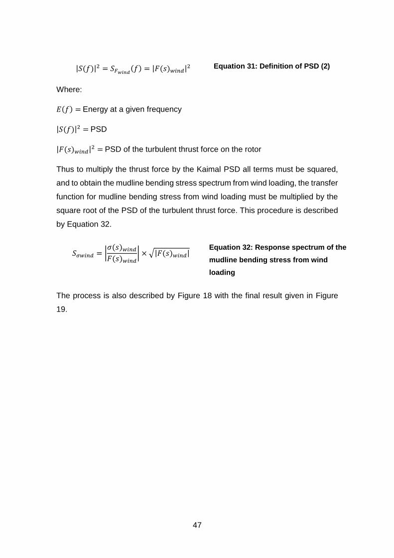
47
|𝑆(𝑓)|2 = 𝑆𝐹𝑤𝑖𝑛𝑑(𝑓) = |𝐹(𝑠)𝑤𝑖𝑛𝑑|2 Equation 31: Definition of PSD (2)
Where:
𝐸(𝑓) = Energy at a given frequency
|𝑆(𝑓)|2 = PSD
|𝐹(𝑠)𝑤𝑖𝑛𝑑|2 = PSD of the turbulent thrust force on the rotor
Thus to multiply the thrust force by the Kaimal PSD all terms must be squared,
and to obtain the mudline bending stress spectrum from wind loading, the transfer
function for mudline bending stress from wind loading must be multiplied by the
square root of the PSD of the turbulent thrust force. This procedure is described
by Equation 32.
𝑆𝜎𝑤𝑖𝑛𝑑 = |𝜎(𝑠)𝑤𝑖𝑛𝑑
𝐹(𝑠)𝑤𝑖𝑛𝑑| × √|𝐹(𝑠)𝑤𝑖𝑛𝑑|
Equation 32: Response spectrum of the
mudline bending stress from wind
loading
The process is also described by Figure 18 with the final result given in Figure
19.
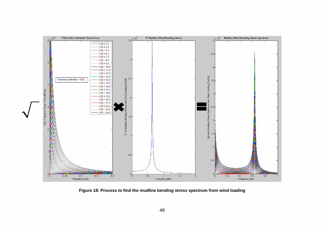
48
Figure 18: Process to find the mudline bending stress spectrum from wind loading
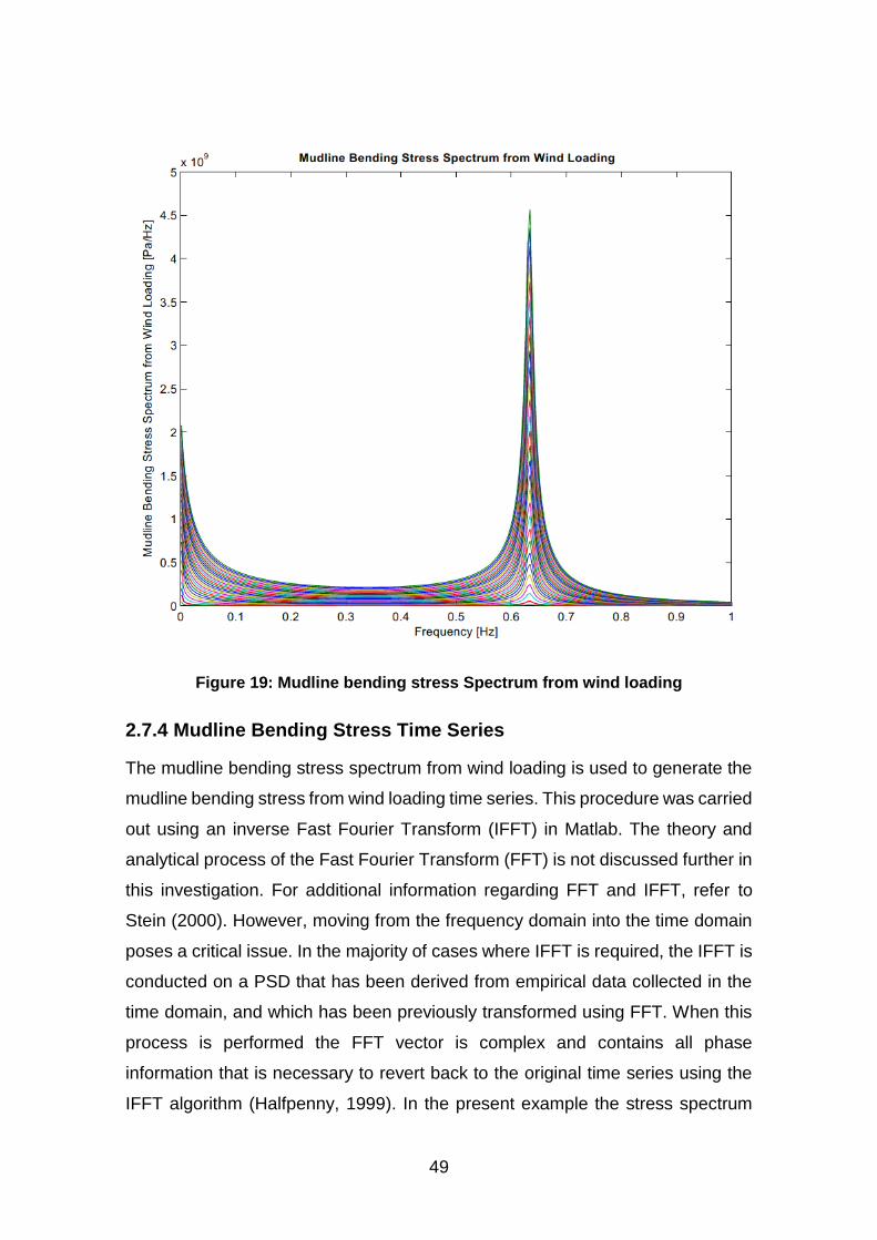
49
Figure 19: Mudline bending stress Spectrum from wind loading
2.7.4 Mudline Bending Stress Time Series
The mudline bending stress spectrum from wind loading is used to generate the
mudline bending stress from wind loading time series. This procedure was carried
out using an inverse Fast Fourier Transform (IFFT) in Matlab. The theory and
analytical process of the Fast Fourier Transform (FFT) is not discussed further in
this investigation. For additional information regarding FFT and IFFT, refer to
Stein (2000). However, moving from the frequency domain into the time domain
poses a critical issue. In the majority of cases where IFFT is required, the IFFT is
conducted on a PSD that has been derived from empirical data collected in the
time domain, and which has been previously transformed using FFT. When this
process is performed the FFT vector is complex and contains all phase
information that is necessary to revert back to the original time series using the
IFFT algorithm (Halfpenny, 1999). In the present example the stress spectrum
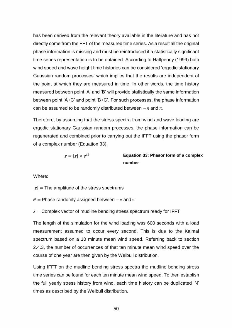
50
has been derived from the relevant theory available in the literature and has not
directly come from the FFT of the measured time series. As a result all the original
phase information is missing and must be reintroduced if a statistically significant
time series representation is to be obtained. According to Halfpenny (1999) both
wind speed and wave height time histories can be considered ‘ergodic stationary
Gaussian random processes’ which implies that the results are independent of
the point at which they are measured in time. In other words, the time history
measured between point ‘A’ and ‘B’ will provide statistically the same information
between point ‘A+C’ and point ‘B+C’. For such processes, the phase information
can be assumed to be randomly distributed between −𝜋 and 𝜋.
Therefore, by assuming that the stress spectra from wind and wave loading are
ergodic stationary Gaussian random processes, the phase information can be
regenerated and combined prior to carrying out the IFFT using the phasor form
of a complex number (Equation 33).
𝑧 = |𝑧| × 𝑒𝑖𝜃 Equation 33: Phasor form of a complex
number
Where:
|𝑧| = The amplitude of the stress spectrums
𝜃 = Phase randomly assigned between −𝜋 and 𝜋
𝑧 = Complex vector of mudline bending stress spectrum ready for IFFT
The length of the simulation for the wind loading was 600 seconds with a load
measurement assumed to occur every second. This is due to the Kaimal
spectrum based on a 10 minute mean wind speed. Referring back to section
2.4.3, the number of occurrences of that ten minute mean wind speed over the
course of one year are then given by the Weibull distribution.
Using IFFT on the mudline bending stress spectra the mudline bending stress
time series can be found for each ten minute mean wind speed. To then establish
the full yearly stress history from wind, each time history can be duplicated ‘N’
times as described by the Weibull distribution.
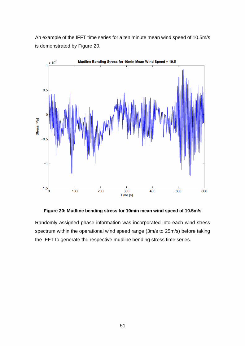
51
An example of the IFFT time series for a ten minute mean wind speed of 10.5m/s
is demonstrated by Figure 20.
Figure 20: Mudline bending stress for 10min mean wind speed of 10.5m/s
Randomly assigned phase information was incorporated into each wind stress
spectrum within the operational wind speed range (3m/s to 25m/s) before taking
the IFFT to generate the respective mudline bending stress time series.
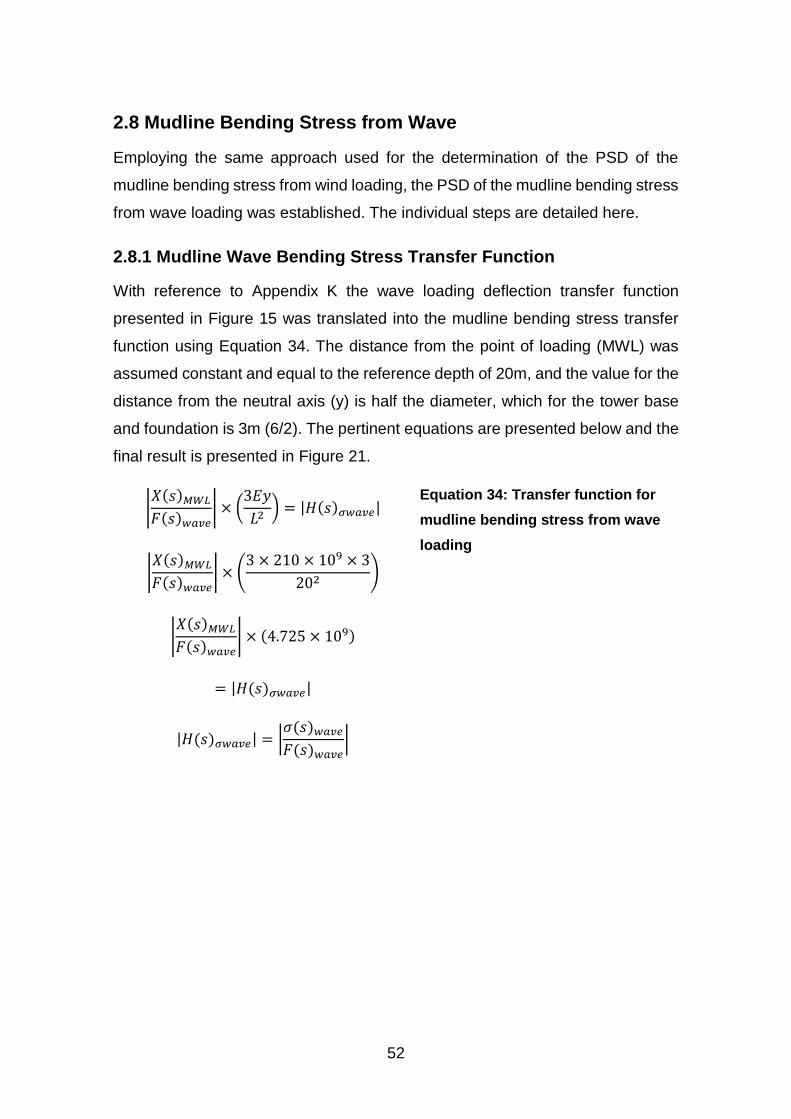
52
2.8 Mudline Bending Stress from Wave
Employing the same approach used for the determination of the PSD of the
mudline bending stress from wind loading, the PSD of the mudline bending stress
from wave loading was established. The individual steps are detailed here.
2.8.1 Mudline Wave Bending Stress Transfer Function
With reference to Appendix K the wave loading deflection transfer function
presented in Figure 15 was translated into the mudline bending stress transfer
function using Equation 34. The distance from the point of loading (MWL) was
assumed constant and equal to the reference depth of 20m, and the value for the
distance from the neutral axis (y) is half the diameter, which for the tower base
and foundation is 3m (6/2). The pertinent equations are presented below and the
final result is presented in Figure 21.
|𝑋(𝑠)𝑀𝑊𝐿
𝐹(𝑠)𝑤𝑎𝑣𝑒| × (
3𝐸𝑦
𝐿2) = |𝐻(𝑠)𝜎𝑤𝑎𝑣𝑒|
|𝑋(𝑠)𝑀𝑊𝐿
𝐹(𝑠)𝑤𝑎𝑣𝑒| × (
3 × 210 × 109 × 3
202)
|𝑋(𝑠)𝑀𝑊𝐿
𝐹(𝑠)𝑤𝑎𝑣𝑒| × (4.725 × 10⁹)
= |𝐻(𝑠)𝜎𝑤𝑎𝑣𝑒|
|𝐻(𝑠)𝜎𝑤𝑎𝑣𝑒| = |𝜎(𝑠)𝑤𝑎𝑣𝑒
𝐹(𝑠)𝑤𝑎𝑣𝑒|
Equation 34: Transfer function for
mudline bending stress from wave
loading
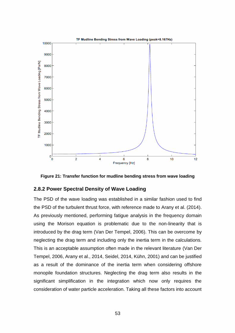
53
Figure 21: Transfer function for mudline bending stress from wave loading
2.8.2 Power Spectral Density of Wave Loading
The PSD of the wave loading was established in a similar fashion used to find
the PSD of the turbulent thrust force, with reference made to Arany et al. (2014).
As previously mentioned, performing fatigue analysis in the frequency domain
using the Morison equation is problematic due to the non-linearity that is
introduced by the drag term (Van Der Tempel, 2006). This can be overcome by
neglecting the drag term and including only the inertia term in the calculations.
This is an acceptable assumption often made in the relevant literature (Van Der
Tempel, 2006, Arany et al., 2014, Seidel, 2014, Kühn, 2001) and can be justified
as a result of the dominance of the inertia term when considering offshore
monopile foundation structures. Neglecting the drag term also results in the
significant simplification in the integration which now only requires the
consideration of water particle acceleration. Taking all these factors into account
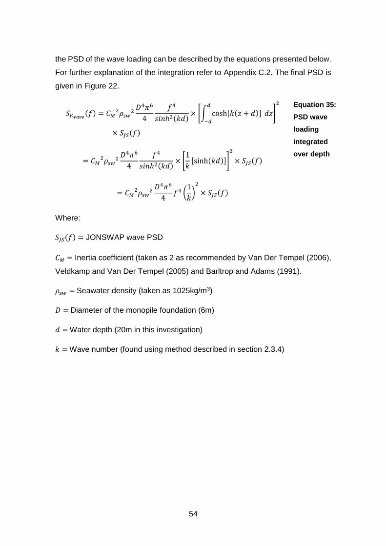
54
the PSD of the wave loading can be described by the equations presented below.
For further explanation of the integration refer to Appendix C.2. The final PSD is
given in Figure 22.
𝑆𝐹𝑤𝑎𝑣𝑒(𝑓) = 𝐶𝑀
2𝜌𝑠𝑤2
𝐷4𝜋6
4
𝑓4
𝑠𝑖𝑛ℎ2(𝑘𝑑)× [∫ cosh[𝑘(𝑧 + 𝑑)]
𝑑
−𝑑
𝑑𝑧]
2
× 𝑆𝐽𝑆(𝑓)
= 𝐶𝑀2𝜌𝑠𝑤
2𝐷4𝜋6
4
𝑓4
𝑠𝑖𝑛ℎ2(𝑘𝑑)× [
1
𝑘[sinh(𝑘𝑑)]]
2
× 𝑆𝐽𝑆(𝑓)
= 𝐶𝑀2𝜌𝑠𝑤
2𝐷4𝜋6
4𝑓4 (
1
𝑘)
2
× 𝑆𝐽𝑆(𝑓)
Equation 35:
PSD wave
loading
integrated
over depth
Where:
𝑆𝐽𝑆(𝑓) = JONSWAP wave PSD
𝐶𝑀 = Inertia coefficient (taken as 2 as recommended by Van Der Tempel (2006),
Veldkamp and Van Der Tempel (2005) and Barltrop and Adams (1991).
𝜌𝑠𝑤 = Seawater density (taken as 1025kg/m3)
𝐷 = Diameter of the monopile foundation (6m)
𝑑 = Water depth (20m in this investigation)
𝑘 = Wave number (found using method described in section 2.3.4)
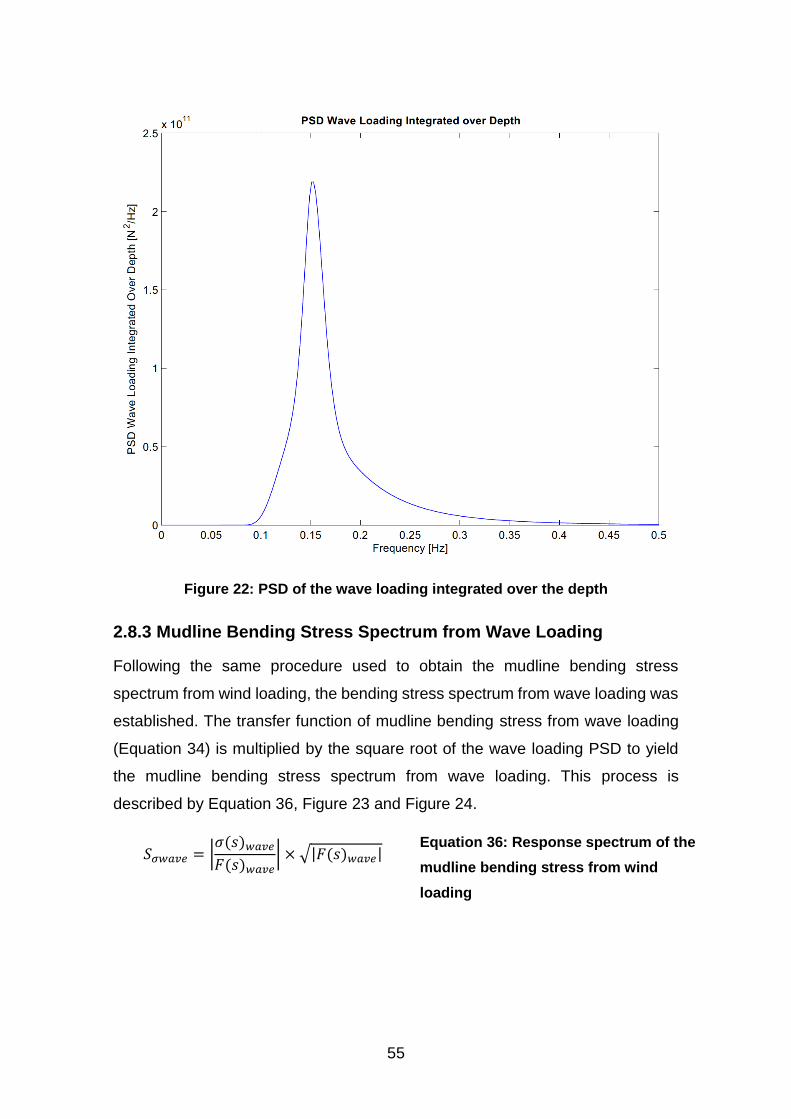
55
Figure 22: PSD of the wave loading integrated over the depth
2.8.3 Mudline Bending Stress Spectrum from Wave Loading
Following the same procedure used to obtain the mudline bending stress
spectrum from wind loading, the bending stress spectrum from wave loading was
established. The transfer function of mudline bending stress from wave loading
(Equation 34) is multiplied by the square root of the wave loading PSD to yield
the mudline bending stress spectrum from wave loading. This process is
described by Equation 36, Figure 23 and Figure 24.
𝑆𝜎𝑤𝑎𝑣𝑒 = |𝜎(𝑠)𝑤𝑎𝑣𝑒
𝐹(𝑠)𝑤𝑎𝑣𝑒| × √|𝐹(𝑠)𝑤𝑎𝑣𝑒|
Equation 36: Response spectrum of the
mudline bending stress from wind
loading
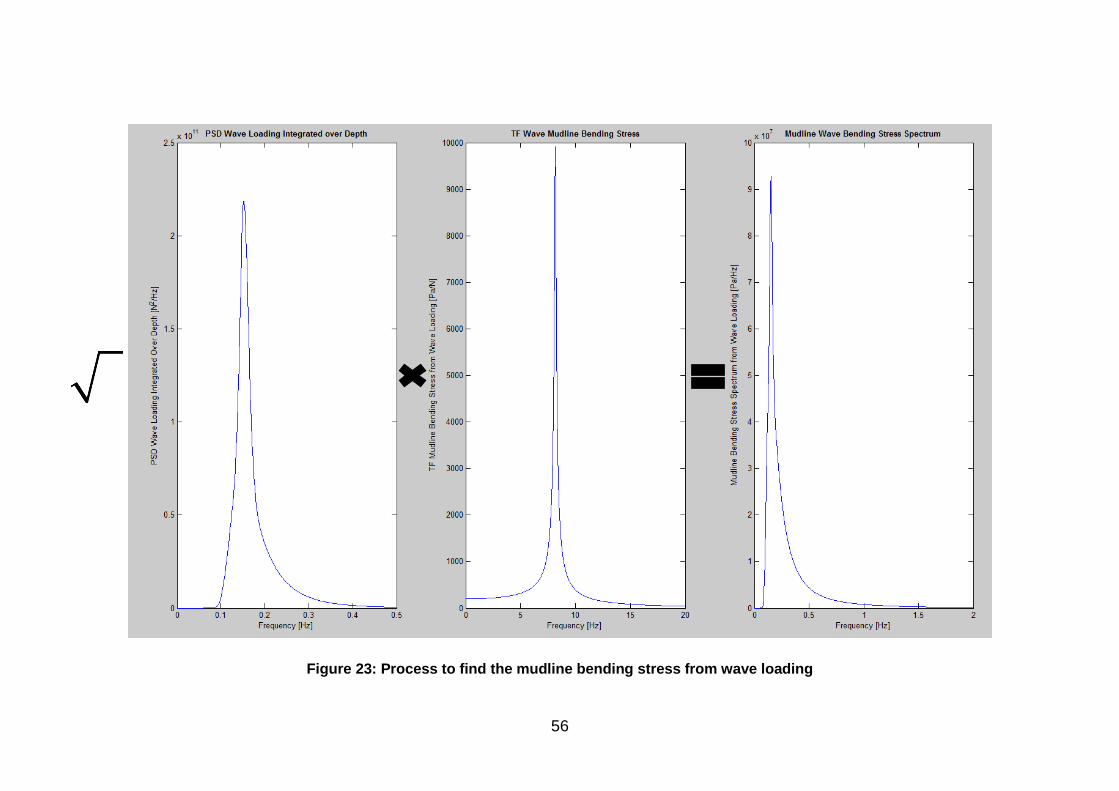
56
Figure 23: Process to find the mudline bending stress from wave loading
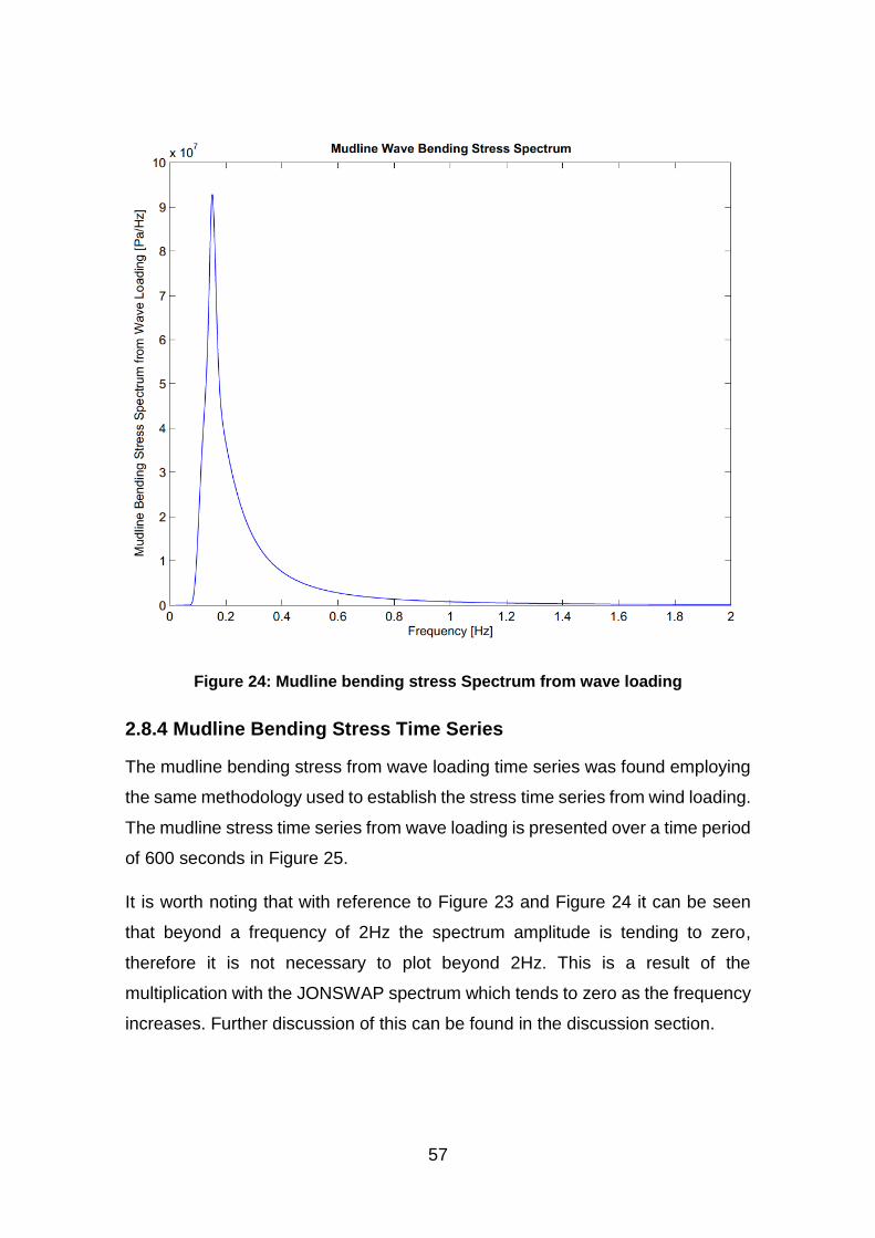
57
Figure 24: Mudline bending stress Spectrum from wave loading
2.8.4 Mudline Bending Stress Time Series
The mudline bending stress from wave loading time series was found employing
the same methodology used to establish the stress time series from wind loading.
The mudline stress time series from wave loading is presented over a time period
of 600 seconds in Figure 25.
It is worth noting that with reference to Figure 23 and Figure 24 it can be seen
that beyond a frequency of 2Hz the spectrum amplitude is tending to zero,
therefore it is not necessary to plot beyond 2Hz. This is a result of the
multiplication with the JONSWAP spectrum which tends to zero as the frequency
increases. Further discussion of this can be found in the discussion section.
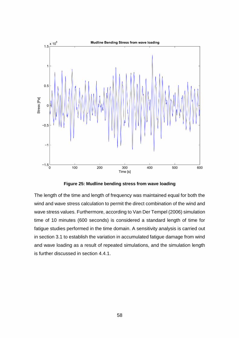
58
Figure 25: Mudline bending stress from wave loading
The length of the time and length of frequency was maintained equal for both the
wind and wave stress calculation to permit the direct combination of the wind and
wave stress values. Furthermore, according to Van Der Tempel (2006) simulation
time of 10 minutes (600 seconds) is considered a standard length of time for
fatigue studies performed in the time domain. A sensitivity analysis is carried out
in section 3.1 to establish the variation in accumulated fatigue damage from wind
and wave loading as a result of repeated simulations, and the simulation length
is further discussed in section 4.4.1.
59
2.9 Rainflow Counting and Damage Equivalent Stress Range
The final step in the process to establish the accumulated fatigue damage of the
reference turbine at the reference site is the calculation of the damage equivalent
stress range value by using Paris Law in combination with a Rainflow counting
algorithm. The methods used to perform this analysis are described in detail by
Pook (2007). The damage equivalent stress range is then used in combination
with a suitable S-N curve to determine the number of life cycles the system can
withstand for the reference conditions. For information regarding the different
types of S-N curves refer to the DNV standard Det Norske Veritas (2012).
As previously mentioned, the S-N curve is plotted on a log-log scale which results
in extreme sensitivity in the final results depending on the S-N curve used. Thus,
to find the number of cycles to failure and the subsequent number of years to
failure, the DNV standard for offshore wind turbine design was referred to. As
recommended by Det Norske Veritas (2014) for offshore wind turbine structures,
the S-N curve in seawater with cathodic protection ‘D’ was selected. The latter
proportion of the curve is used when >106 cycles can be expected which results
in a Paris coefficient of 5 and a log �̅� value of 15.606. The latter proportion of
the curve was used in this investigation due to the high number of cycles the
system is expected to endure throughout its design life. Note that a value of 5 for
the Paris exponent has been assumed throughout. Appendix M presents further
information regarding suggested S-N curves and Figure 2 found in section 1.2.1
depicts the plots.
60
2.10 Wind and Wave Loading Superposition
Superposition of the wind and wave loading is a topic of discussion in the
literature and many approaches to perform this operation have been proposed
(Kühn 2001). An objective of this investigation was to establish how different wind
and wave superposition methodologies effect the final system fatigue life. To
address this objective the following approaches were used.
The first superposition method, discussed by Kühn (2001) and Van Der Tempel
(2006), suggests that the bending stress spectra determined for both wind and
waves can be combined (summed) prior to establishing the damage equivalent
stress range. At this point, there are two options for the spectral superposition:
in-phase, or out-of-phase superposition (see Figure 29). Van Der Tempel (2006)
does not specify which should be used, while Kühn (2001) has considered both.
Both have been considered in this investigation, however, it is evident that in-
phase will yield a more conservative result than the out-of-phase method. The
out-of-phase approach is closer to reality as a result of its ability to take into
account, to some extent, the out-of-phase wind and wave loading conditions.
Thus, for this investigation, the random phase component has been added
separately to wind and wave mudline bending spectra before IFFT and prior to
the spectra superposition. This results in a partial cancellation of a proportion of
the amplification which would otherwise occur with the application of equal phase
data. The difference in the final result, with and without the application of
difference phase information is presented in Table 7 and discussed further in the
discussion chapter.
The next method compared is Kühn’s unweighted equivalent method which was
shown to provide accurate results with a 3% error and at least as accurate as any
alternative method (Kühn, 2001). The final approach directly combines the
damage equivalent stress range values from wind and waves.
The final method directly combines the separate damage equivalent stress
ranges after Rainflow Counting and is included for comparative purposes.
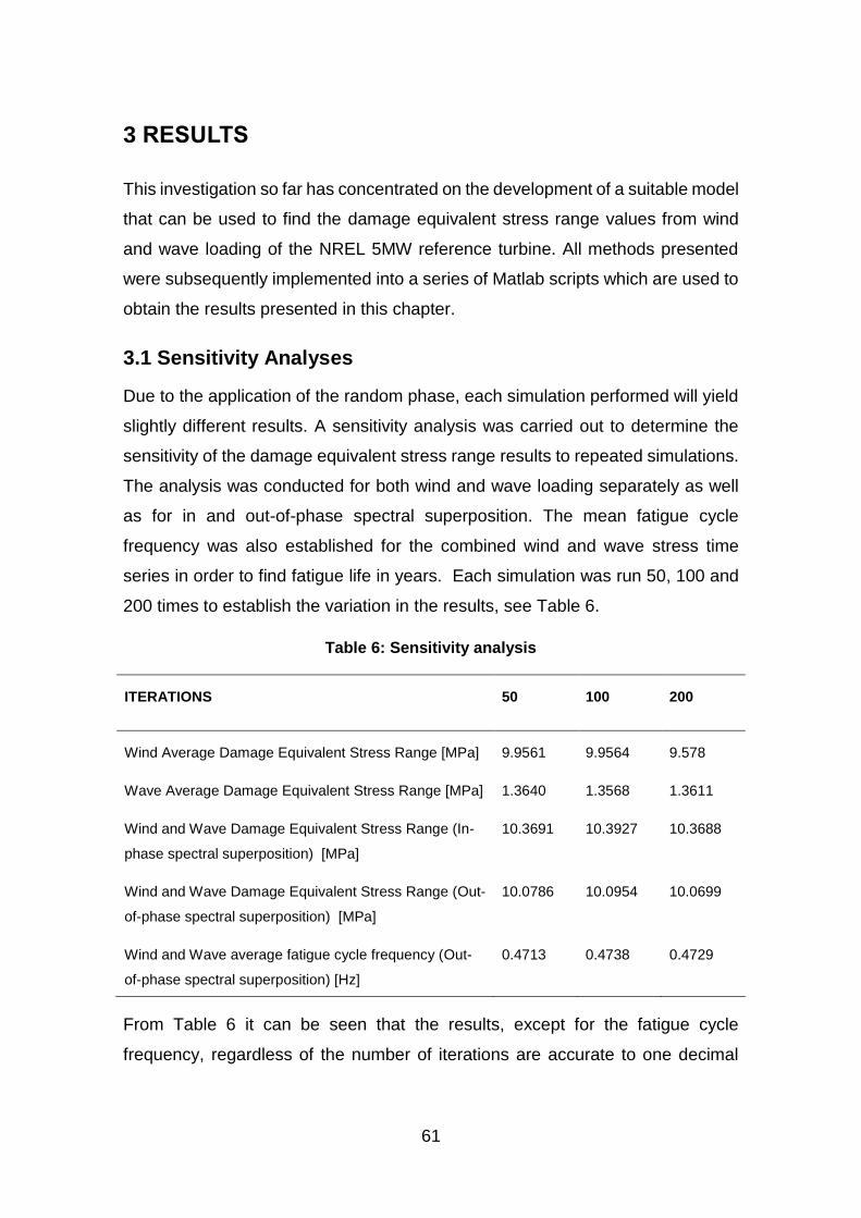
61
3 RESULTS
This investigation so far has concentrated on the development of a suitable model
that can be used to find the damage equivalent stress range values from wind
and wave loading of the NREL 5MW reference turbine. All methods presented
were subsequently implemented into a series of Matlab scripts which are used to
obtain the results presented in this chapter.
3.1 Sensitivity Analyses
Due to the application of the random phase, each simulation performed will yield
slightly different results. A sensitivity analysis was carried out to determine the
sensitivity of the damage equivalent stress range results to repeated simulations.
The analysis was conducted for both wind and wave loading separately as well
as for in and out-of-phase spectral superposition. The mean fatigue cycle
frequency was also established for the combined wind and wave stress time
series in order to find fatigue life in years. Each simulation was run 50, 100 and
200 times to establish the variation in the results, see Table 6.
Table 6: Sensitivity analysis
ITERATIONS 50 100 200
Wind Average Damage Equivalent Stress Range [MPa] 9.9561 9.9564 9.578
Wave Average Damage Equivalent Stress Range [MPa] 1.3640 1.3568 1.3611
Wind and Wave Damage Equivalent Stress Range (In-
phase spectral superposition) [MPa]
10.3691 10.3927 10.3688
Wind and Wave Damage Equivalent Stress Range (Out-
of-phase spectral superposition) [MPa]
10.0786 10.0954 10.0699
Wind and Wave average fatigue cycle frequency (Out-
of-phase spectral superposition) [Hz]
0.4713 0.4738 0.4729
From Table 6 it can be seen that the results, except for the fatigue cycle
frequency, regardless of the number of iterations are accurate to one decimal
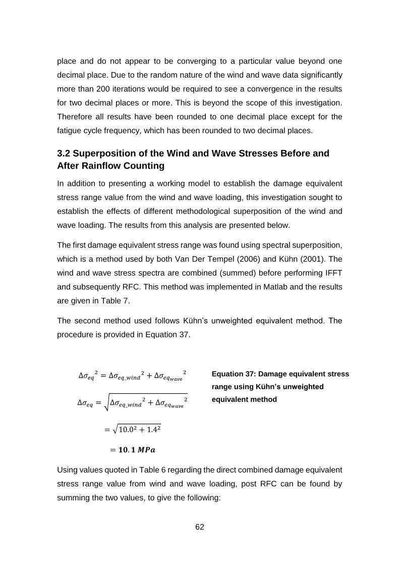
62
place and do not appear to be converging to a particular value beyond one
decimal place. Due to the random nature of the wind and wave data significantly
more than 200 iterations would be required to see a convergence in the results
for two decimal places or more. This is beyond the scope of this investigation.
Therefore all results have been rounded to one decimal place except for the
fatigue cycle frequency, which has been rounded to two decimal places.
3.2 Superposition of the Wind and Wave Stresses Before and
After Rainflow Counting
In addition to presenting a working model to establish the damage equivalent
stress range value from the wind and wave loading, this investigation sought to
establish the effects of different methodological superposition of the wind and
wave loading. The results from this analysis are presented below.
The first damage equivalent stress range was found using spectral superposition,
which is a method used by both Van Der Tempel (2006) and Kühn (2001). The
wind and wave stress spectra are combined (summed) before performing IFFT
and subsequently RFC. This method was implemented in Matlab and the results
are given in Table 7.
The second method used follows Kühn’s unweighted equivalent method. The
procedure is provided in Equation 37.
∆𝜎𝑒𝑞2 = ∆𝜎𝑒𝑞_𝑤𝑖𝑛𝑑
2 + ∆𝜎𝑒𝑞𝑤𝑎𝑣𝑒
2
∆𝜎𝑒𝑞 = √∆𝜎𝑒𝑞_𝑤𝑖𝑛𝑑2 + ∆𝜎𝑒𝑞𝑤𝑎𝑣𝑒
2
= √10.02 + 1.42
= 𝟏𝟎. 𝟏 𝑴𝑷𝒂
Equation 37: Damage equivalent stress
range using Kühn’s unweighted
equivalent method
Using values quoted in Table 6 regarding the direct combined damage equivalent
stress range value from wind and wave loading, post RFC can be found by
summing the two values, to give the following:

63
∆𝜎𝑒𝑞 = ∆𝜎𝑒𝑞_𝑤𝑖𝑛𝑑 + ∆𝜎𝑒𝑞𝑤𝑎𝑣𝑒
= 10.0 + 1.4
= 𝟏𝟏. 𝟒 𝑴𝑷𝒂
Equation 38: Damage equivalent stress
range direct superposition
3.3 Summary of Results
Table 7 provides a summary of the results and includes an estimate of the
number of cycles to failure as well as the estimated fatigue life in years. As
previously mentioned, the number of cycles to failure have been estimated using
S-N curve ‘D’ as suggested in DNV J101 offshore standard (Det Norske Veritas,
2014). See Appendix M for further details.
The general formula for the S-N curve is given by Equation 39.
log 𝑁 = log �̅� − 𝑚 log ∆𝜎 Equation 39: SN curve
The fatigue life in years was established by determining the number of fatigue
cycles within the mudline bending stress time series for the given time period.
The calculated mean frequency of the fatigue cycles from wind and wave was
found to be 0.47Hz rounded to 2 decimal places (see Table 6). A summary of the
final results is provided in Table 7 on the following page which are subsequently
discussed in the proceeding discussion chapter.
64
Table 7: Results summary table
Method Description Out-of-phase Spectra
Superposition Before
RFC
Unweighted
Equivalent
Superposition After
RFC
In-phase Spectra
Superposition
Before RFC
Direct Superposition
After RFC
Damage equivalent
stress range from wind
and wave loads [MPa]
10.1 10.1 10.4 11.4
Number of fatigue
cycles to failure (using
curve ‘D’)
3.84 x10¹⁰ 3.84 x10¹⁰ 3.32 x10¹⁰ 2.10 x10¹⁰
Fatigue life [years] 2591 2591 2238 1417
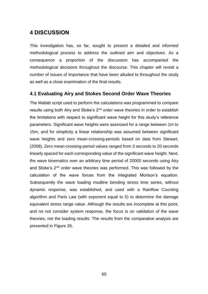
65
4 DISCUSSION
This investigation has, so far, sought to present a detailed and informed
methodological process to address the outlined aim and objectives. As a
consequence a proportion of the discussion has accompanied the
methodological decisions throughout the discourse. This chapter will revisit a
number of issues of importance that have been alluded to throughout the study
as well as a close examination of the final results.
4.1 Evaluating Airy and Stokes Second Order Wave Theories
The Matlab script used to perform the calculations was programmed to compare
results using both Airy and Stoke’s 2nd order wave theories in order to establish
the limitations with respect to significant wave height for this study’s reference
parameters. Significant wave heights were assessed for a range between 1m to
15m, and for simplicity a linear relationship was assumed between significant
wave heights and zero mean-crossing-periods based on data from Stewart,
(2008). Zero mean-crossing-period values ranged from 3 seconds to 20 seconds
linearly spaced for each corresponding value of the significant wave height. Next,
the wave kinematics over an arbitrary time period of 20000 seconds using Airy
and Stoke’s 2nd order wave theories was performed. This was followed by the
calculation of the wave forces from the integrated Morison’s equation.
Subsequently the wave loading mudline bending stress time series, without
dynamic response, was established, and used with a Rainflow Counting
algorithm and Paris Law (with exponent equal to 5) to determine the damage
equivalent stress range value. Although the results are incomplete at this point,
and no not consider system response, the focus is on validation of the wave
theories, not the loading results. The results from the comparative analysis are
presented in Figure 26.
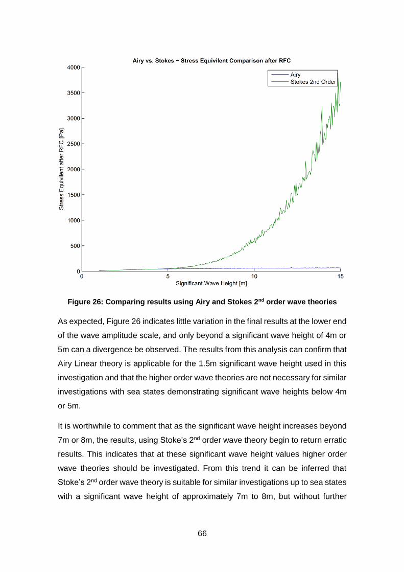
66
Figure 26: Comparing results using Airy and Stokes 2nd order wave theories
As expected, Figure 26 indicates little variation in the final results at the lower end
of the wave amplitude scale, and only beyond a significant wave height of 4m or
5m can a divergence be observed. The results from this analysis can confirm that
Airy Linear theory is applicable for the 1.5m significant wave height used in this
investigation and that the higher order wave theories are not necessary for similar
investigations with sea states demonstrating significant wave heights below 4m
or 5m.
It is worthwhile to comment that as the significant wave height increases beyond
7m or 8m, the results, using Stoke’s 2nd order wave theory begin to return erratic
results. This indicates that at these significant wave height values higher order
wave theories should be investigated. From this trend it can be inferred that
Stoke’s 2nd order wave theory is suitable for similar investigations up to sea states
with a significant wave height of approximately 7m to 8m, but without further
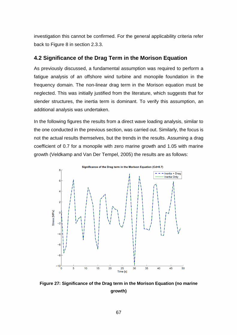
67
investigation this cannot be confirmed. For the general applicability criteria refer
back to Figure 8 in section 2.3.3.
4.2 Significance of the Drag Term in the Morison Equation
As previously discussed, a fundamental assumption was required to perform a
fatigue analysis of an offshore wind turbine and monopile foundation in the
frequency domain. The non-linear drag term in the Morison equation must be
neglected. This was initially justified from the literature, which suggests that for
slender structures, the inertia term is dominant. To verify this assumption, an
additional analysis was undertaken.
In the following figures the results from a direct wave loading analysis, similar to
the one conducted in the previous section, was carried out. Similarly, the focus is
not the actual results themselves, but the trends in the results. Assuming a drag
coefficient of 0.7 for a monopile with zero marine growth and 1.05 with marine
growth (Veldkamp and Van Der Tempel, 2005) the results are as follows:
Figure 27: Significance of the Drag term in the Morison Equation (no marine
growth)
68
Figure 28: Significance of the Drag term in the Morison Equation (with marine
growth)
Figure 27 and Figure 28 indicate almost complete agreement between the cases
where the drag is included and where the drag is excluded. It was also found that
even by increasing the drag coefficient to 1.05 to account for possible marine
growth, the drag remained negligible. These results indicate that the fundamental
assumption on which this investigation has been based is valid for the selected
reference parameters. The point at which the drag begins to become significant
is hugely dependent on the specific parameters of the particular study and include
the drag coefficient, the structural geometry, and the sea state conditions. Given
the importance of frequency domain analysis for the offshore industry, this
investigation suggests that future studies that explore the limits of validity for this
fundamental assumption would be beneficial.
4.3 Fatigue Loading Regimes
Loading of offshore wind turbines and monopile foundations consist of a variety
of complex loading regimes. This investigation has observed the two most
significant of these: loading from wind and waves (Passon and Branner, 2014).
69
In addition, the wave loading has been limited to the inertia component, excluding
drag, diffraction, slap and slam and vortex shedding induced oscillatory loading,
all of which contribute to the complete wave loading regime (Barltrop and Adams,
1991). Supplementary neglected components include loading from currents, wind
shear, shaft tilt, tower shadow (Burton et al., 2011), yaw error, yaw motion, gravity
as well as the momentary loading as a result of wind gusts, vibrations from
turbine start and stop and any resonance induced loading (Manwell et al., 2009).
As previously mentioned, to accommodate all the possible loading regimes
requires significantly detailed information regarding all aspects of the system and
deployment site. Such an analysis would need to be carried out in the time
domain to include the non-linear loading interactions (Van Der Tempel, 2006).
Consequently the analysis would require significant computational and time
resources. This kind of study is far beyond the scope of this investigation and it
has been shown that for design purposes, linearized approaches are acceptable
(Det Norske Veritas, 2014, Van Der Tempel, 2006, Yeter et al., 2014, Seidel,
2014). To some extent, the non-conservative approach of neglecting such non-
linearities will be mitigated by adopting a conservative collinear wind and wave
direction assumption. This assumption is acceptable for locations where the
prevailing winds are onshore, but becomes less acceptable for locations
frequently experiencing offshore winds (Arany et al., 2014). That said, it should
be noted, if a 90° misalignment occurs between the wind and wave direction,
minimal damping prevails and such conditions will govern the fatigue design
(Passon and Branner, 2014). Again, more detailed information regarding the
specific installation site is required to take these additional factors into
consideration.
4.4 Results
The accuracy of the results from this investigation are invariably proportional to
the legitimacy of the assumptions and the limitations inherent in the employed
methodology. Some of the major assumptions have already been discussed in
the preceding sections, however further discussion on a number of issues will be
presented here with respect to the final results.
70
4.4.1 Simulation Length
As previously discussed, the standard simulation length is 10 minutes (600
seconds) which is the length employed throughout this investigation. However,
according to a consensus group of experts in the field, this length should be
increased to between 1200 seconds to 3600 seconds (Van Der Tempel, 2006).
Furthermore, due to the IFFT procedure used, the frequency vector resolution
was chosen to correspond to the simulation length required (i.e. 600 points). This
investigation choose not to increase the simulation length, due primarily, to the
additional computational resources which were found to increase exponentially
with simulation length. In addition, the wave stress spectrum was determined only
once for a 600 second time period and repeated ‘N’ – number of times as required
by the Weibull distribution analysis. It is suggested that with additional time and
computational resources, this study would benefit from a more detailed and
comprehensive sensitivity analysis that considers the effects of increasing the
simulation time length and varying the frequency vector resolution.
Despite the limitations in the methodologies, this investigation was careful to
follow standard practise which deems 600 seconds sufficient (Van Der Tempel,
2006) and that the length of the frequency vector should be adequate to maintain
the details contained within the spectral shape (Barltrop and Adams, 1991). To
verify the latter has been upheld, all spectra used have been plotted and provided
throughout this study or in the relevant appendices.
4.4.2 Spectral Multiplication
In section 2.8.4, the mudline bending stress spectrum from wave loading was
described. The methodology chose to ignore all frequencies beyond 2Hz as a
result of the propensity of the JONSWAP spectrum to tend to zero as the
frequency increases. As a result, the system excitation from wave loading is
relatively small. The system’s displacement transfer function from wave loading
was found to have a peak frequency of 8.186Hz, which is at a significant distance
from the peak frequencies of the JONSWAP spectrum which occurs, for the
reference parameters, at around 0.15Hz. Consequently, a significant proportion
of the response spectrum is cancelled out. If sea state parameters decrease the
71
JONSWAP peak frequency will increase and less cancellation will occur,
however, significant decreases are unlikely for the North Sea, which suggests
that system resonance from waves is unlikely.
4.4.3 System Response
Another potential source of error, with respect to wind and wave loading, are the
methods used to establish system response. As previously mentioned, data
regarding the peak frequency of the tower top displacement transfer function, was
taken directly from the literature, applied to this study, and used to establish the
system’s stiffness. Making the necessary assumptions, this was in turn used to
find the system stiffness at the mean water level and the subsequent response
from wave loading. Although the peak frequency of the transfer function found in
the literature was quoted for the NREL 5MW reference turbine, the methods used
to establish this transfer function and the detailed parameters and assumptions
on which it was based, were not explored further. Herein lies an area of great
uncertainty, and without significant time and investment to verify this assumption,
the data presented from the wind and wave loading analysis must be approached
with caution. To improve confidence in the results, a complete and detailed Finite
Element Analysis is suggested, which can be used to establish a significantly
more accurate estimation of the system’s stiffness and subsequently the
response transfer functions.
4.4.4 Final Results Analysis
The first two methods of superposition used in this study were the out-of-phase
spectral superposition, and Kühn’s unweighted equivalent method. These two
methods were selected on the basis of their proven accuracy and validity (Van
Der Tempel, 2006, Kühn, 2001). Interestingly, the results from these two
approaches were found to return exactly the same result, when rounded to one
decimal place. According to Kühn (2001), this is expected due to Pythagoras’s
law which can be considered as an out-of-phase superposition of the damage
equivalent stress range values. For a further discussion of Kühn’s method and
its derivation refer to Kühn (2001). As expected the final results from these two
methods are the least conservative, and are thought to provide the most realistic
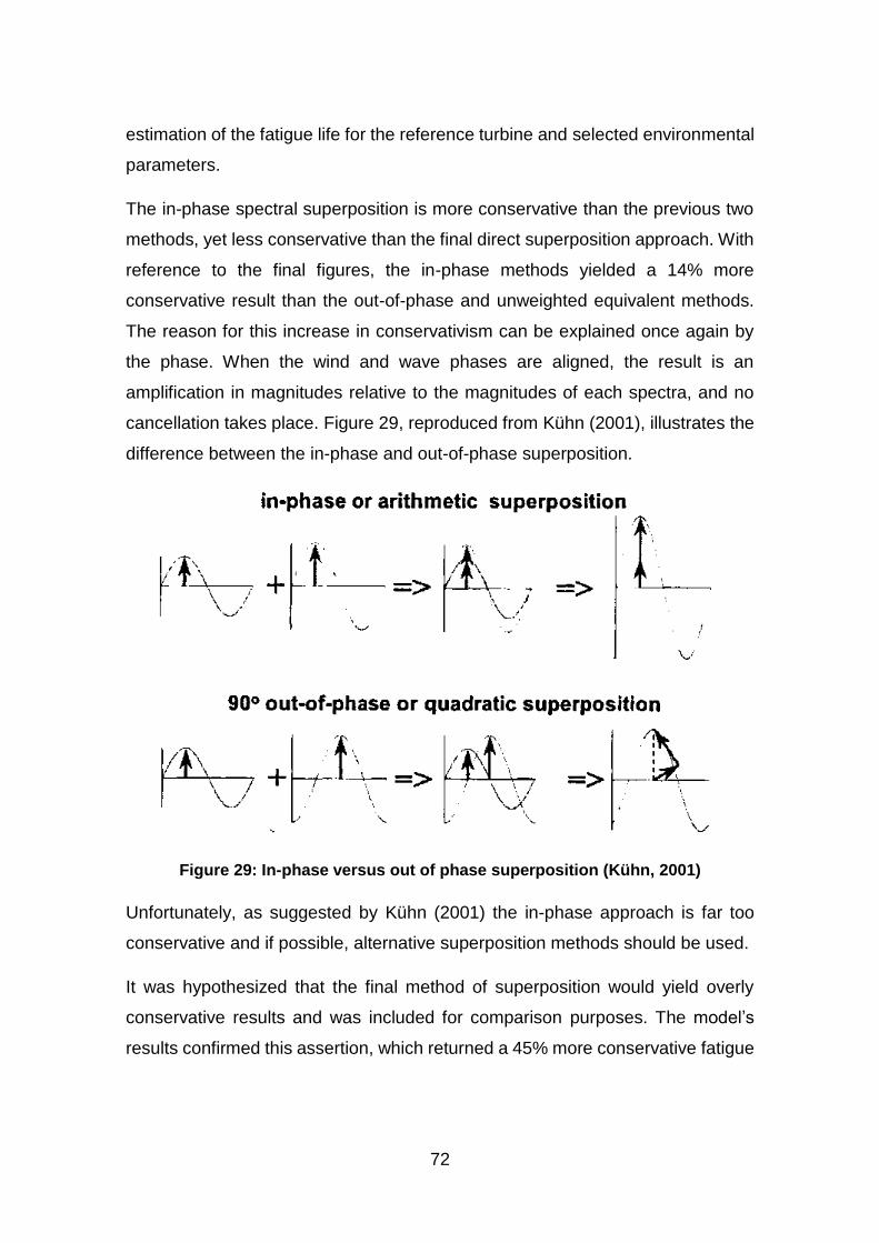
72
estimation of the fatigue life for the reference turbine and selected environmental
parameters.
The in-phase spectral superposition is more conservative than the previous two
methods, yet less conservative than the final direct superposition approach. With
reference to the final figures, the in-phase methods yielded a 14% more
conservative result than the out-of-phase and unweighted equivalent methods.
The reason for this increase in conservativism can be explained once again by
the phase. When the wind and wave phases are aligned, the result is an
amplification in magnitudes relative to the magnitudes of each spectra, and no
cancellation takes place. Figure 29, reproduced from Kühn (2001), illustrates the
difference between the in-phase and out-of-phase superposition.
Figure 29: In-phase versus out of phase superposition (Kühn, 2001)
Unfortunately, as suggested by Kühn (2001) the in-phase approach is far too
conservative and if possible, alternative superposition methods should be used.
It was hypothesized that the final method of superposition would yield overly
conservative results and was included for comparison purposes. The model’s
results confirmed this assertion, which returned a 45% more conservative fatigue
73
life estimation than the results from the out-of-phase and unweighted equivalent
approaches.
Before carrying out the various superposition approaches, a prediction of the
outcomes was established from data available in the literature. Using methods
that are known to be less accurate than others may appear counterproductive,
however, this was undertaken to verify, to some extent, that the model is capable
of returning values that are in line with what is expected for a given methodology.
This final point becomes even more significant when direct result comparison
from similar investigations was, regrettably, not possible. This is due to the very
specific nature of every fatigue analyses performed for the offshore wind industry
and the confidential nature of the findings. Consequently, no publicly available
comparative data could be found, to the Author’s knowledge. Subsequently a
complete model validation was not possible, and is suggested as an area for
future investigations.
Although the results appear to conform to the methodological expectations from
the superposition processes, the model has also returned higher than expected
fatigue live predictions for the offshore wind turbine and monopile foundation
structure. The precise reason for this, is regrettably beyond the scope of this
investigation, however it is likely that an accumulation of assumptions made
throughout the methodological process has a significant effect on the final fatigue
figures. However, these assumptions were imperative in order to proceed through
the analysis and to establish a working fatigue model. As previously stated, it is
speculated that the un-verified assumption pertaining to the system stiffness
presents a very large area of uncertainty. With additional time, sensitivity
analyses could contribute to the verification or rejection of such unverified
assumptions and help to establish how variable the end fatigue life is to
fluctuations in each assumption made.
Finally, it is also worth noting, that similar investigations of this nature, rarely use
IFFT to return to the time domain for the determination of the damage equivalent
stress range, as there are accepted methods to obtain this directly from the
superimposed stress spectrum (Van Der Tempel, 2006). It would therefore be of

74
great interest, to future studies, to compare frequency domain damage equivalent
stress range calculations with IFFT and RFC derived damage equivalent stress
range, to identify any discrepancies and explore their possible reasons.
Despite the limitations discussed in this chapter, every care has been taken to
verify, where reasonably possible, that the Matlab scripts used to generate and
process data, are returning reasonable results for that specified methodology,
theory and known input parameters. These verifications have been presented
and discussed throughout the entirety of this investigation.
4.5 Areas for Future Investigations
Throughout the execution of this research project, areas deemed worthy of further
attention have been noted and are summarised in this section below:
The effects of neglecting a transition piece on the fatigue life
How many iterations are required to observe a convergence in the damage
stress equivalent values to more than one decimal place
Given the importance of frequency domain analysis for the offshore industry,
this investigation suggests that future studies that explore the limits of validity
for this fundamental assumption would be beneficial
FEA analysis to establish system stiffness and subsequent model validation.
Explore the limits of validity of neglecting wave drag in the frequency domain
calculation of fatigue life
Run the model for a known case with known and detailed parameters to
establish validity
Identify the extent of discrepancies in the damage equivalent stress range
values from using conventional frequency domain methods and the less
conventional IFFT with RFC method used in this investigation
Further sensitivity analyses with the purpose of establishing the sensitivity of
the fatigue life to the effects of each un-verified assumption made
75
5 CONCLUSIONS
The aim of this study was to present a numerical model for the fatigue analysis
of offshore wind turbines with monopile foundations. This investigation has
achieved the outlined aim, addressed all stated objectives and presented and
discussed the methodologies and findings. The outcomes from the study agree
with data presented in the literature and indicate that there is no difference
between using the out-of-phase spectral superposition or Kühn’s unweighted
equivalent method when rounded to one decimal place. This agreement in the
results provides confidence for the methodological processes used however, the
unrealistically augmented final fatigue life has raised questions regarding the
validity of a number of the assumptions. To validate the model and to increase
confidence in the assumptions it is suggested that significantly more detailed
information is required and that further sensitivity analyses should be performed.
In conclusion, the model presented in this investigation is the result of extensive
and detailed research that draws on a wide variety of technical resources to arrive
at a working offshore wind turbine fatigue model. Although the model has its
limitations it is now in a strong position to be taken forward as the basis for future
investigations looking into the fatigue lives of offshore wind turbines. With the
number of offshore wind farms increasing, and with deeper water and harsher
conditions expected, it is imperative that fatigue life investigations continue to
ensure system safety and economic viability is maintained for the foreseeable
future.

77
REFERENCES
ABP MER 2008. Atlas of UK Marine Renewable Energy Resources: Technical Report. Hampshire, UK: ABP Marine Environmental Research Ltd.
ARANY, L., BHATTACHARYA, S., MACDONALD, J. & HOGAN, S. J. 2014. Simplified critical mudline bending moment spectra of offshore wind turbine support structures. Wind Energy, n/a-n/a.
BARLTROP, N. D. P. & ADAMS, A. J. 1991. Dynamics of Fixed Marine Structures (Third Edition), Butterworth-Heinemann.
BENDAT, J. S. & PIERSOL, A. G. 1993. Engineering applications of correlation and spectral analysis, USA, J. Wiley.
BRETON, S.-P. & MOE, G. 2009. Status, plans and technologies for offshore wind turbines in Europe and North America. Renewable Energy, 34, 646-654.
BURTON, T., JENKINS, N., SHARPE, D. & BOSSANYI, E. 2011. Wind Energy Handbook, Wiley.
BUSBY, R. L. 2012. Wind Power: The Industry Grows Up, PennWell Corporation.
CHAKRABARTI, S. K. 2005. Handbook of Offshore Engineering, Oxford, Elsevier.
DECC, U. 2011. Renewable Energy Roadmap. Department of Energy and Climate Change, London.
DET NORSKE VERITAS 2010. Environmental Conditions and Environmental Loads. DNV-RP-C205. Norway: Det Norske Veritas.
DET NORSKE VERITAS 2012. Fatigue Design of Offshore Steel Structures. DNV-RP-C203. Norway: Det Norske Veritas.
DET NORSKE VERITAS 2014. Design of Offshore Wind Turbine Structures. DNV-OS-J101. Norway: Det Norske Veritas.
DONG, W., MOAN, T. & GAO, Z. 2011. Long-term fatigue analysis of multi-planar tubular joints for jacket-type offshore wind turbine in time domain. Engineering Structures, 33, 2002-2014.
EEA 2009. Europe's onshore and offshore wind energy potential: An assessment of environmental and economic constraints. Copenhagen: European Environment Agency.
EWEA 2013. Deep Water: The next step for offshore wind energy. Brussels, Belgium: A report by the European Wind Energy Association. EU: European Wind Energy Association.
78
EWEA 2015. Wind in Power: 2014 European statistics. THE EUROPEAN WIND ENERGY ASSOCIATION.
FONTANA, C. 2014. Development of a methodology for the preliminary estimation of the loads on the mooring system of a taut moored tidal device. Master of Science, Cranfield University.
FROHBOESE, P., SCHMUCK, C. & HASSAN, G. G. 2010. Thrust coefficients used for estimation of wake effects for fatigue load calculation. European Wind Energy Conference, 2010 Warsaw, Poland. Poland, 1-10.
GERE, J. & GOODNO, B. 2009. Mechanics of Materials, USA, Cengage Learning.
GSANGER, S. & PITTELOUD, J. 2013. World Wind Energy Report 2012. World Wind Energy Association. Bonn, Germany: World Wind Energy Association WWEA 2013.
HALFPENNY, A. A Frequency Domain Approach for Fatigue Life Estimation from Finite Element Analysis. Key Engineering Materials, 1999. Trans Tech Publ, 401-410.
IEC 2009. Wind Turbine—Part 1: Design Requirements (3rd edn.). Geneva, Switzerland: International Electrotechnical Commission.
JONKMAN, J. M. 2007. Dynamics modeling and loads analysis of an offshore floating wind turbine, ProQuest.
JONKMAN, J. M., BUTTERFIELD, S., MUSIAL, W. & SCOTT, G. 2009. Definition of a 5-MW Reference Wind Turbine for Offshore System Development. USA: National Renewable Energy Laboratory.
JUSTUS, C. G. 1978. Winds and wind system performance, Franklin Institute Press.
KÜHN, M. J. 2001. Dynamics and design optimisation of offshore wind energy conversion systems. PhD, TU Delft University.
LLOYD, G. 2000. Rules & Guidelines 2000: IV Non-marine Technology-Regulations for the Certification of (Offshore) Wind Energy Conversion Systems.
LYNN, P. A. 2011. Onshore and Offshore Wind Energy: An Introduction, Wiley.
LYSEN, E. H. 1983. Introduction to Wind Energy: Basic and Advanced Introduction to Wind Energy with Emphasis on Water Pumping Windmills, CWD- Consultancy Services Wind Energy Developing Countries.
MACKAY, D. 2008. Sustainable Energy-without the hot air, UIT Cambridge.
79
MANWELL, J. F., MCGOWAN, J. G. & ROGERS, A. L. 2009. Wind Energy Explained: Theory, Design and Application, Wiley.
MARGARITI, G., PAPADOPOULOS, A., BARMPAS, D., GANTES, C. J. & GKOLOGIANNIS, P. 2015. Design of Monopile and Tripod Foundation of Fixed Offshore Wind Turbines via Advanced Numerical Analysis. 8th GRACM International Congress on Computational Mechanics.
MUSIAL, W. 2011. Large-Scale Offshore Wind Power in the United States: Assessment of Oppportunities and Barriers, DIANE Publishing Company.
PASSON, P. 2015. Damage equivalent wind–wave correlations on basis of damage contour lines for the fatigue design of offshore wind turbines. Renewable Energy, 81, 723-736.
PASSON, P. & BRANNER, K. 2014. Condensation of long-term wave climates for the fatigue design of hydrodynamically sensitive offshore wind turbine support structures. Ships and Offshore Structures, 1-25.
PATEL, M. H. 1989. Dynamics of Offshore Structures, UK, Butterworth-Heinemann.
POOK, L. P. 2007. Metal Fatigue: What It Is, Why It Matters, Springer Netherlands.
PYTEL, A. & KIUSALAAS, J. 2011. Mechanics of Materials, Cengage Learning.
RENEWABLE UK. 2014. UK Wind Energy Database (UKWED) [Online]. UK: Renewable UK. Available: http://www.renewableuk.com/en/renewable-energy/wind-energy/uk-wind-energy-database/ [Accessed 8 Feb 2014].
SEIDEL, M. 2014. Wave induced fatigue loads: Insights from frequency domain calculations. Stahlbau, 83, 535-541.
SEIDEL, M., VON MUTIUS, M. & STEUDEL, D. Design and load calculations for offshore foundations of a 5 MW turbine. Conference proceedings DEWEK, 2004. 351-356.
STEIN, J. 2000. Digital Signal Processing: A Computer Science Perspective, USA, John Wiley & Sons, Inc.
THE CROWN ESTATE 2013. Offshore wind operational report 2013. London.
TUPPER, E. 1996. Introduction to Naval Architecture, Oxford, UK, Butterworth Heinemann.
VAN DER TEMPEL, J. 2006. Design of support structures for offshore wind turbines. PhD, TU Delft, Delft University of Technology.
VELDKAMP, H. F. & VAN DER TEMPEL, J. 2005. Influence of wave modelling on the prediction of fatigue for offshore wind turbines. Wind Energy, 8, 49-65.

80
YETER, B., GARBATOV, Y. & SOARES, C. G. 2014. Spectral fatigue assessment of an offshore wind turbine structure under wave and wind loading. Developments in Maritime Transportation and Exploitation of Sea Resources, 425-433.
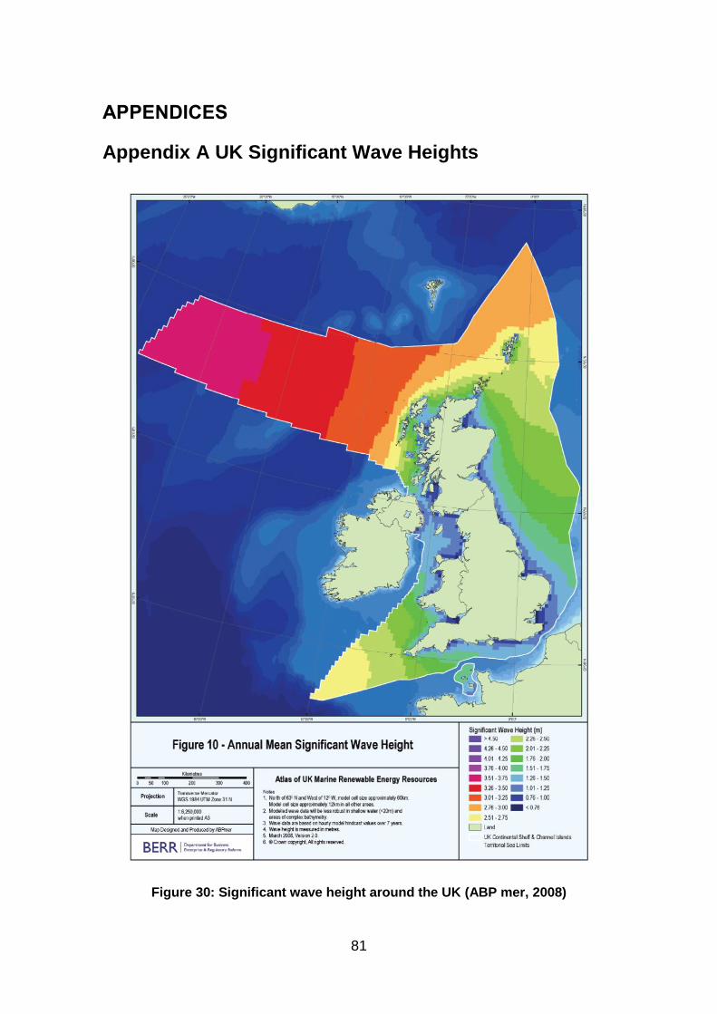
81
APPENDICES
Appendix A UK Significant Wave Heights
Figure 30: Significant wave height around the UK (ABP mer, 2008)
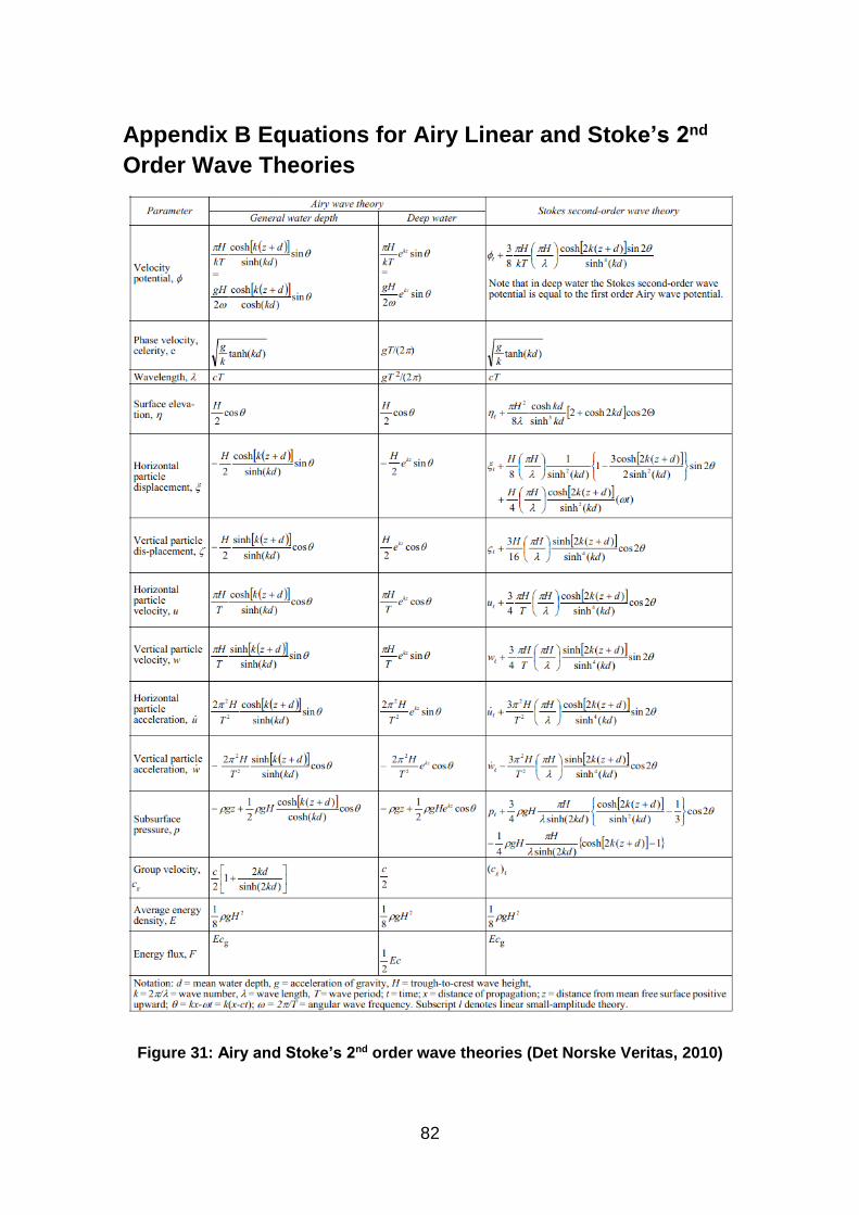
82
Appendix B Equations for Airy Linear and Stoke’s 2nd
Order Wave Theories
Figure 31: Airy and Stoke’s 2nd order wave theories (Det Norske Veritas, 2010)
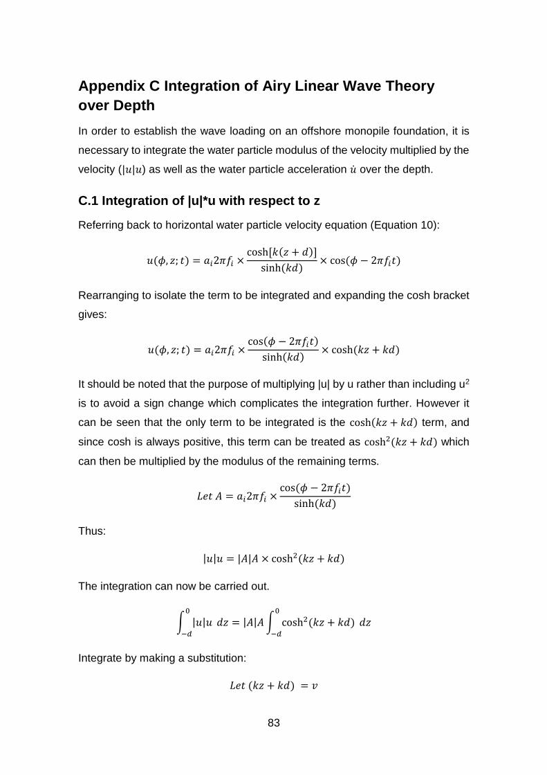
83
Appendix C Integration of Airy Linear Wave Theory
over Depth
In order to establish the wave loading on an offshore monopile foundation, it is
necessary to integrate the water particle modulus of the velocity multiplied by the
velocity (|𝑢|𝑢) as well as the water particle acceleration �̇� over the depth.
C.1 Integration of |u|*u with respect to z
Referring back to horizontal water particle velocity equation (Equation 10):
𝑢(𝜙, 𝑧; 𝑡) = 𝑎𝑖2𝜋𝑓𝑖 ×cosh [𝑘(𝑧 + 𝑑)]
sinh (𝑘𝑑)× cos (𝜙 − 2𝜋𝑓𝑖𝑡)
Rearranging to isolate the term to be integrated and expanding the cosh bracket
gives:
𝑢(𝜙, 𝑧; 𝑡) = 𝑎𝑖2𝜋𝑓𝑖 ×cos(𝜙 − 2𝜋𝑓𝑖𝑡)
sinh(𝑘𝑑)× cosh (𝑘𝑧 + 𝑘𝑑)
It should be noted that the purpose of multiplying |u| by u rather than including u2
is to avoid a sign change which complicates the integration further. However it
can be seen that the only term to be integrated is the cosh(𝑘𝑧 + 𝑘𝑑) term, and
since cosh is always positive, this term can be treated as cosh2 (𝑘𝑧 + 𝑘𝑑) which
can then be multiplied by the modulus of the remaining terms.
𝐿𝑒𝑡 𝐴 = 𝑎𝑖2𝜋𝑓𝑖 ×cos (𝜙 − 2𝜋𝑓𝑖𝑡)
sinh (𝑘𝑑)
Thus:
|𝑢|𝑢 = |𝐴|𝐴 × cosh2 (𝑘𝑧 + 𝑘𝑑)
The integration can now be carried out.
∫ |𝑢|𝑢0
−𝑑
𝑑𝑧 = |𝐴|𝐴 ∫ cosh2 (𝑘𝑧 + 𝑘𝑑) 0
−𝑑
𝑑𝑧
Integrate by making a substitution:
𝐿𝑒𝑡 (𝑘𝑧 + 𝑘𝑑) = 𝑣

84
Cannot directly integrate cosh2(𝑣) refer to trigonometric identities. Note:
cosh(𝑣) =𝑒𝑣 + 𝑒−𝑣
2
And that:
cosh2(𝑣) = (𝑒𝑣 + 𝑒−𝑣
2)
2
cosh2(𝑣) =1
4× (𝑒𝑣 + 𝑒−𝑣)2
Expanding the brackets gives:
cosh2(𝑣) =1
4(𝑒2𝑣 + 2 + 𝑒−2𝑣)
Substituting back into the integral:
∫ |𝑢|𝑢0
−𝑑
𝑑𝑧 = |𝐴|𝐴 ×1
4∫ (𝑒2𝑣 + 2 + 𝑒−2𝑣)
0
−𝑑
𝑑𝑧
Need to different (𝑘𝑧 + 𝑘𝑑) to make the 𝑣 the subject of the integration:
𝑑𝑣
𝑑𝑧= 𝑘
𝑑𝑧 =𝑑𝑣
𝑘
Thus:
∫ |𝑢|𝑢0
−𝑑
𝑑𝑧 = |𝐴|𝐴 ×1
4𝑘∫ (𝑒2𝑣 + 2 + 𝑒−2𝑣)
0
−𝑑
𝑑𝑣
Integration can now take place:
∫ |𝑢|𝑢0
−𝑑
𝑑𝑧 = |𝐴|𝐴 ×1
4𝑘× [
1
2𝑒2𝑣 + 2𝑣 −
1
2𝑒−2𝑣]
−𝑑
0
Simplifying slightly gives:
85
∫ |𝑢|𝑢0
−𝑑
𝑑𝑧 = |𝐴|𝐴 ×1
8𝑘× [𝑒2𝑣 + 4𝑣 − 𝑒−2𝑣]−𝑑
0
Before substitute back in for 𝑣 convert back to a trigonometric term if possible:
sinh(𝑣) =𝑒𝑣 − 𝑒−𝑣
2
2sinh(2𝑣) = 𝑒2𝑣 − 𝑒−2𝑣
Thus:
∫ |𝑢|𝑢0
−𝑑
𝑑𝑧 = |𝐴|𝐴 ×1
8𝑘× [2sinh(2𝑣) + 4𝑣]−𝑑
0
Substituting back in for 𝑣:
∫ |𝑢|𝑢0
−𝑑
𝑑𝑧 = |𝐴|𝐴 ×1
8𝑘× [2sinh[2(𝑘𝑧 + 𝑘𝑑)] + 4(𝑘𝑧 + 𝑘𝑑)]−𝑑
0
Finally:
∫ |𝑢|𝑢0
−𝑑
𝑑𝑧 = |𝐴|𝐴 ×1
8𝑘× [2sinh(2𝑘𝑧 + 2𝑘𝑑) + (4𝑘𝑧 + 4𝑘𝑑)]−𝑑
0
Apply the limits gives:
∫ |𝑢|𝑢0
−𝑑
𝑑𝑧 = |𝐴|𝐴 ×1
8𝑘× [2sinh(2𝑘𝑑) + 4𝑘𝑑]
This is the final equation used for |𝑢|𝑢 in the Morison Equation.
C.2 Integration of water particle acceleration with respect to z
The same procedure was employed for the water particle acceleration given that
exactly the same term in the equation is integrated, (cosh [𝑘(𝑧 + 𝑑)]).
Thus:
∫ �̇�0
−𝑑
𝑑𝑧 = 𝑎𝑖(2𝜋𝑓𝑖)2 ×sin (𝜙 − 2𝜋𝑓𝑖𝑡)
sinh (𝑘𝑑)× ∫ cosh [𝑘(𝑧 + 𝑑)]
𝑑
−𝑑
𝑑𝑧

86
Which can be performed by substituting (𝑘𝑧 + 𝑘𝑑) = 𝑣.
∫ �̇�0
−𝑑
𝑑𝑧 = 𝑎𝑖(2𝜋𝑓𝑖)2 ×sin (𝜙 − 2𝜋𝑓𝑖𝑡)
sinh (𝑘𝑑)× ∫ cosh(𝑣) 𝑑𝑧
𝑑
−𝑑
∫ �̇�0
−𝑑
𝑑𝑧 = 𝑎𝑖(2𝜋𝑓𝑖)2 ×
sin (𝜙 − 2𝜋𝑓𝑖𝑡)
sinh (𝑘𝑑)×
1
𝑘∫ cosh(𝑣) 𝑑𝑣
𝑑
−𝑑
∫ �̇�0
−𝑑
𝑑𝑧 = 𝑎𝑖(2𝜋𝑓𝑖)2 ×sin (𝜙 − 2𝜋𝑓𝑖𝑡)
sinh (𝑘𝑑)×
1
𝑘[sinh(𝑣)]−𝑑
0
Applying the limits and substituting back in for 𝑣:
∫ �̇�0
−𝑑
𝑑𝑧 = 𝑎𝑖(2𝜋𝑓𝑖)2 ×
sin (𝜙 − 2𝜋𝑓𝑖𝑡)
sinh (𝑘𝑑)×
1
𝑘[sinh(𝑘𝑧 + 𝑘𝑑)]−𝑑
0
∫ �̇�0
−𝑑
𝑑𝑧 = 𝑎𝑖(2𝜋𝑓𝑖)2 ×sin (𝜙 − 2𝜋𝑓𝑖𝑡)
sinh (𝑘𝑑)×
1
𝑘[sinh(𝑘𝑑)]
Cancelling the sinh terms gives:
∫ �̇�0
−𝑑
𝑑𝑧 = 𝑎𝑖(2𝜋𝑓𝑖)2 ×sin (𝜙 − 2𝜋𝑓𝑖𝑡)
𝑘
87
Appendix D Integration of Stoke’s 2nd Order Wave
Theory over Depth
D.1 Integration of |u|*u according to Stoke’s 2nd Order Wave
Theory over Depth
Once Airy theory has been integrated over the depth Stokes theory can be easily
integrated by modifying the same equations used to integrate Airy. This is
possible due to only very minor differences in the integrand. The final integration
of stokes is presented below.
Stoke’s 2nd order wave water particle velocity is given as:
𝑢𝑆𝑡𝑜𝑘𝑒′𝑠 = 𝑢𝐴𝑖𝑟𝑦 +3𝑎𝑖
2𝜋2𝑓𝑖
𝜆×
cos[2(𝜙 − 2𝜋𝑓𝑖𝑡)]
sinh4(𝑘𝑑)× cosh [2(𝑘𝑧 + 𝑘𝑑)]
To integrate let:
3𝑎𝑖2𝜋2𝑓𝑖
𝜆×
cos[2(𝜙 − 2𝜋𝑓𝑖𝑡)]
sinh4(𝑘𝑑)= 𝐵
Therefore:
∫ |𝑢|𝑢𝑆𝑡𝑜𝑘𝑒′𝑠
0
−𝑑
𝑑𝑧
= ∫ |𝑢|𝑢𝐴𝑖𝑟𝑦
0
−𝑑
𝑑𝑧 + |𝐵|𝐵 ×1
16𝑘
× [2sinh(4𝑘𝑧 + 4𝑘𝑑) + (8𝑘𝑧 + 8𝑘𝑑)]−𝑑0
Giving:
∫ |𝑢|𝑢𝑆𝑡𝑜𝑘𝑒′𝑠
0
−𝑑
𝑑𝑧 = ∫ |𝑢|𝑢𝐴𝑖𝑟𝑦
0
−𝑑
𝑑𝑧 + |𝐵|𝐵 ×1
16𝑘× [2sinh(4𝑘𝑑) + (8𝑘𝑑)]
D.2 Integration of water particle acceleration according to
Stoke’s 2nd Order Wave Theory over Depth
Following the same process as described above the water particle acceleration
can be integrated over the water depth relatively easily.
88
Stoke’s 2nd order wave water acceleration is given as:
�̇�𝑆𝑡𝑜𝑘𝑒′𝑠 = �̇�𝐴𝑖𝑟𝑦 +12𝑎𝑖
2𝜋3𝑓𝑖2
𝜆×
sin[2(𝜙 − 2𝜋𝑓𝑖𝑡)]
sinh4(𝑘𝑑)× cosh [2(𝑘𝑧 + 𝑘𝑑)]
Integration becomes:
∫ �̇�𝑆𝑡𝑜𝑘𝑒′𝑠
0
−𝑑
𝑑𝑧
= ∫ �̇�𝐴𝑖𝑟𝑦
0
−𝑑
𝑑𝑧 +12𝑎𝑖
2𝜋3𝑓𝑖2
𝜆×
sin[2(𝜙 − 2𝜋𝑓𝑖𝑡)]
sinh4(𝑘𝑑)
× ∫ cosh[2(𝑘𝑧 + 𝑘𝑑)] 𝑑𝑧0
−𝑑
Integrating and applying the limits yields:
∫ �̇�𝑆𝑡𝑜𝑘𝑒′𝑠
0
−𝑑
𝑑𝑧 = ∫ �̇�𝐴𝑖𝑟𝑦
0
−𝑑
𝑑𝑧 +12𝑎𝑖
2𝜋3𝑓𝑖2
𝜆×
sin[2(𝜙 − 2𝜋𝑓𝑖𝑡)]
sinh4(𝑘𝑑)×
1
2𝑘sinh(2𝑘𝑑)
These equations are then used in the Morison Equation to determine the total
wave force on the monopile.

89
Appendix E Actuator Disk Theory
It is known that the power coefficient (Cp) is represented by Equation 40, where
𝑃 is the power of the rotor.
𝐶𝑃 =𝑃
1
2𝜌𝑎𝐴𝑟𝑜𝑡𝑜𝑟𝑈3
Equation 40: Power coefficient (1)
And that the power of the rotor is described by:
𝑃 =1
2𝜌𝑎𝐴𝑟𝑜𝑡𝑜𝑟𝑈3[4𝑎(1 − 𝑎)2] Equation 41: Rotor power
Thus equating Equation 40 and Equation 41 gives:
𝐶𝑃 = 4𝑎(1 − 𝑎)2 Equation 42: Power coefficient (2)
If it was possible to extract 100% of the wind energy Cp would equal 0.59,
however this is highly unlikely with the maximum efficiency achieved by large
scale wind turbines currently around 50% (Cp = 0.5) (Lynn, 2011). Therefore, if
an assumption is made regarding the turbine power coefficient, the value of the
axial induction factor can be found iteratively. Taking NREL turbine power
coefficient equal 0.482 (Jonkman et al., 2009), the axial induction factor was
found iteratively as 0.1785973 (see Table 8 below).
Table 8: Finding the axial induction factor for a turbine with a Cp=0.482
Cp a Desired Cp
0.5625 0.25 0.482
0.554496 0.24
0.545468 0.23
0.535392 0.22
0.524244 0.21
0.512 0.2
0.498636 0.19
0.484128 0.18
0.482613356 0.179
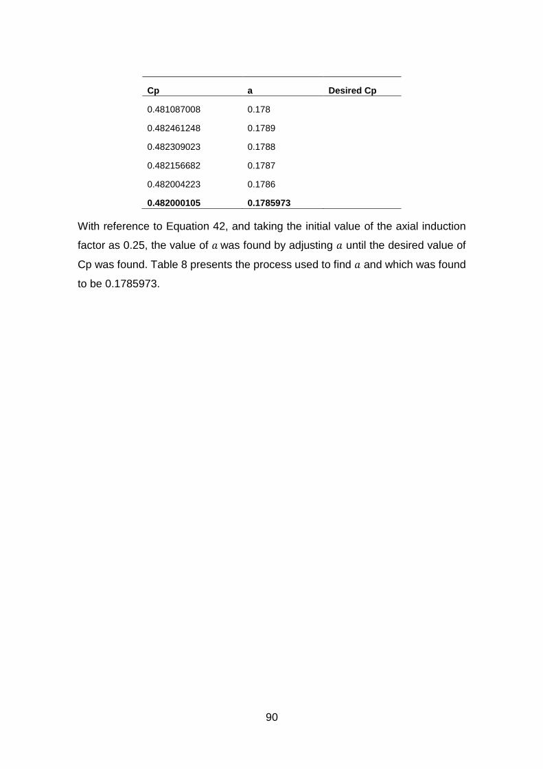
90
Cp a Desired Cp
0.481087008 0.178
0.482461248 0.1789
0.482309023 0.1788
0.482156682 0.1787
0.482004223 0.1786
0.482000105 0.1785973
With reference to Equation 42, and taking the initial value of the axial induction
factor as 0.25, the value of 𝑎 was found by adjusting 𝑎 until the desired value of
Cp was found. Table 8 presents the process used to find 𝑎 and which was found
to be 0.1785973.
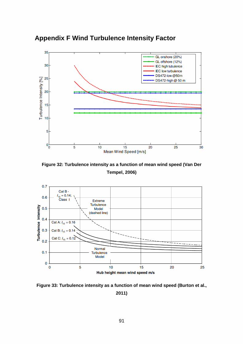
91
Appendix F Wind Turbulence Intensity Factor
Figure 32: Turbulence intensity as a function of mean wind speed (Van Der
Tempel, 2006)
Figure 33: Turbulence intensity as a function of mean wind speed (Burton et al.,
2011)
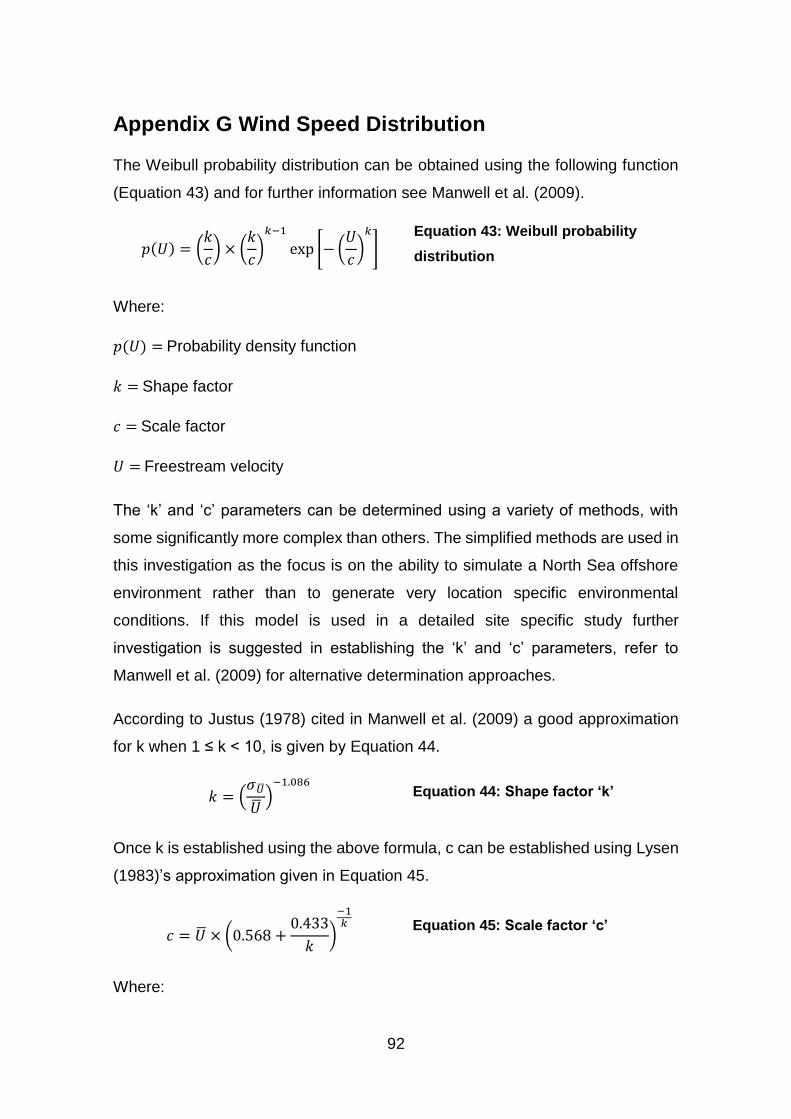
92
Appendix G Wind Speed Distribution
The Weibull probability distribution can be obtained using the following function
(Equation 43) and for further information see Manwell et al. (2009).
𝑝(𝑈) = (𝑘
𝑐) × (
𝑘
𝑐)
𝑘−1
exp [− (𝑈
𝑐)
𝑘
] Equation 43: Weibull probability
distribution
Where:
𝑝(𝑈) = Probability density function
𝑘 = Shape factor
𝑐 = Scale factor
𝑈 = Freestream velocity
The ‘k’ and ‘c’ parameters can be determined using a variety of methods, with
some significantly more complex than others. The simplified methods are used in
this investigation as the focus is on the ability to simulate a North Sea offshore
environment rather than to generate very location specific environmental
conditions. If this model is used in a detailed site specific study further
investigation is suggested in establishing the ‘k’ and ‘c’ parameters, refer to
Manwell et al. (2009) for alternative determination approaches.
According to Justus (1978) cited in Manwell et al. (2009) a good approximation
for k when 1 ≤ k < 10, is given by Equation 44.
𝑘 = (𝜎�̅�
�̅�)
−1.086
Equation 44: Shape factor ‘k’
Once k is established using the above formula, c can be established using Lysen
(1983)’s approximation given in Equation 45.
𝑐 = �̅� × (0.568 +0.433
𝑘)
−1𝑘
Equation 45: Scale factor ‘c’
Where:
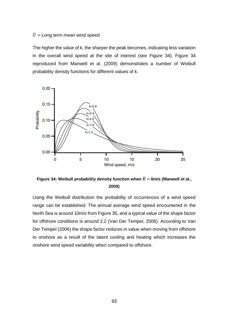
93
�̅� = Long term mean wind speed
The higher the value of k, the sharper the peak becomes, indicating less variation
in the overall wind speed at the site of interest (see Figure 34). Figure 34
reproduced from Manwell et al. (2009) demonstrates a number of Weibull
probability density functions for different values of k.
Figure 34: Weibull probability density function when �̅� = 6m/s (Manwell et al.,
2009)
Using the Weibull distribution the probability of occurrences of a wind speed
range can be established. The annual average wind speed encountered in the
North Sea is around 10m/s from Figure 35, and a typical value of the shape factor
for offshore conditions is around 2.2 (Van Der Tempel, 2006). According to Van
Der Tempel (2006) the shape factor reduces in value when moving from offshore
to onshore as a result of the latent cooling and heating which increases the
onshore wind speed variability when compared to offshore.
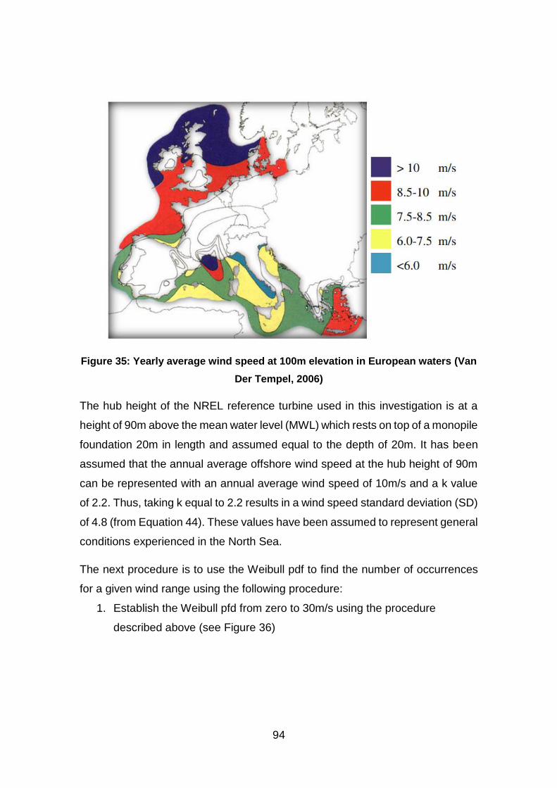
94
Figure 35: Yearly average wind speed at 100m elevation in European waters (Van
Der Tempel, 2006)
The hub height of the NREL reference turbine used in this investigation is at a
height of 90m above the mean water level (MWL) which rests on top of a monopile
foundation 20m in length and assumed equal to the depth of 20m. It has been
assumed that the annual average offshore wind speed at the hub height of 90m
can be represented with an annual average wind speed of 10m/s and a k value
of 2.2. Thus, taking k equal to 2.2 results in a wind speed standard deviation (SD)
of 4.8 (from Equation 44). These values have been assumed to represent general
conditions experienced in the North Sea.
The next procedure is to use the Weibull pdf to find the number of occurrences
for a given wind range using the following procedure:
1. Establish the Weibull pfd from zero to 30m/s using the procedure
described above (see Figure 36)
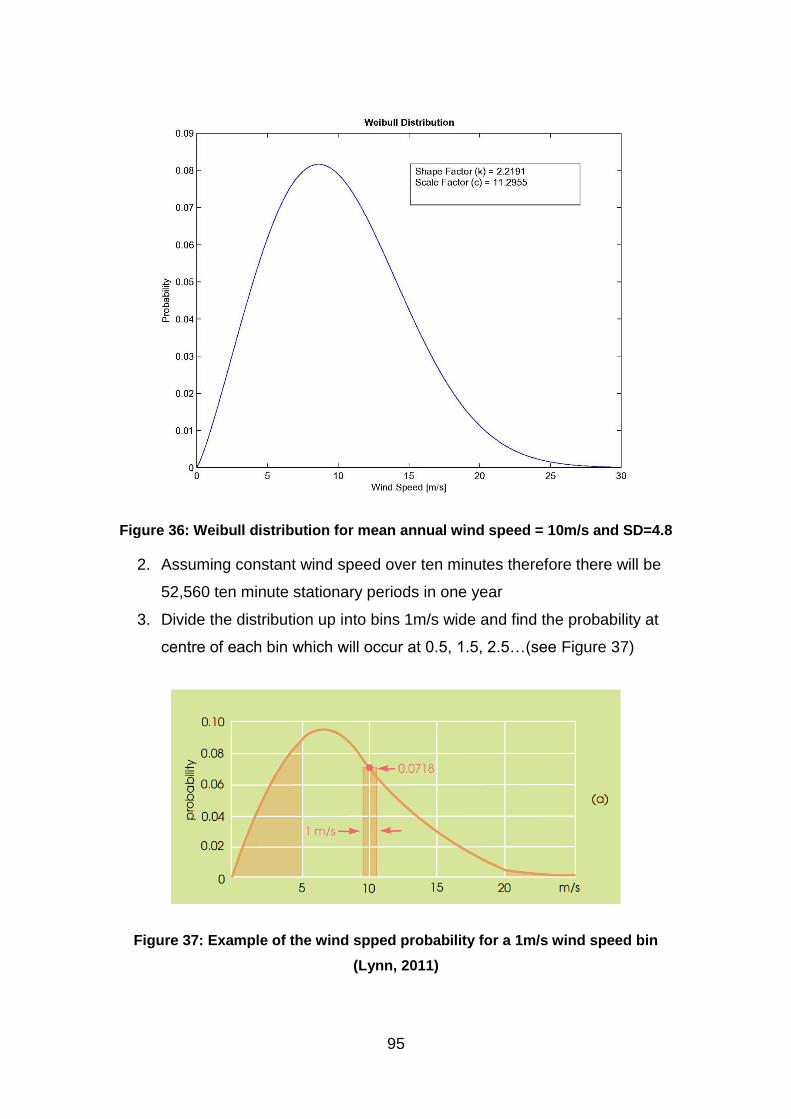
95
Figure 36: Weibull distribution for mean annual wind speed = 10m/s and SD=4.8
2. Assuming constant wind speed over ten minutes therefore there will be
52,560 ten minute stationary periods in one year
3. Divide the distribution up into bins 1m/s wide and find the probability at
centre of each bin which will occur at 0.5, 1.5, 2.5…(see Figure 37)
Figure 37: Example of the wind spped probability for a 1m/s wind speed bin
(Lynn, 2011)

96
4. Multiply the probability of each bin centre by the number of ten minute
stationary periods in one year to yield the number of times that the
specific wind speed range is experienced in the course of one year (see
Figure 11).
5. Employ the actuator disk theory to find the thrust of the wind turbine at
each mean bin wind speed

97
Appendix H Wind Turbulence
The process used to generate the Kaimal spectrum is given here, as
recommended in the relevant standard DNV J101 (Det Norske Veritas, 2014).
𝑆�̅�10(𝑓) = 𝜎2
4𝐿𝑘
�̅�10
(1 +6𝑓𝐿𝑘
�̅�10)
5/3 Equation 46: Kaimal spectrum
𝐿𝑘 = 5.67𝑧 𝑓𝑜𝑟 𝑧 < 60𝑚
and
𝐿𝑘 = 340.2𝑚 𝑓𝑜𝑟 𝑧 ≥ 60𝑚
Equation 47: Integral scale
parameter
Where:
𝑆�̅�10(𝑓) = Kaimal PSD at a given mean wind speed
𝑓 = Frequency
𝐿𝑘 = Integral scale parameter
In order to plot the spectrum the standard deviation for a given ten minute wind
stationary period must be determined.
With reference to the turbulence intensity equation (Equation 20), this
investigation has established the standard deviation over the full range of ten
minute mean wind speeds taking the turbulence intensity factor at a constant
value of 12%. Assuming a turbine hub height greater than 60m and a constant
turbulence intensity of 12% Figure 12 demonstrates the Kiamal PSD for mean
wind speeds from 3.5m/s (3m/s = cut in speed) to 24.5m/s (25m/s = cut out
speed).
An example of the wind speed turbulence for mean wind speeds from 0.5m/s to
29.5m/s with 1m/s interval bins is given in the following three figures.
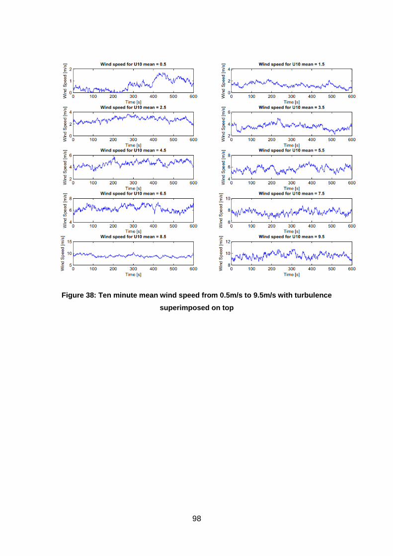
98
Figure 38: Ten minute mean wind speed from 0.5m/s to 9.5m/s with turbulence
superimposed on top
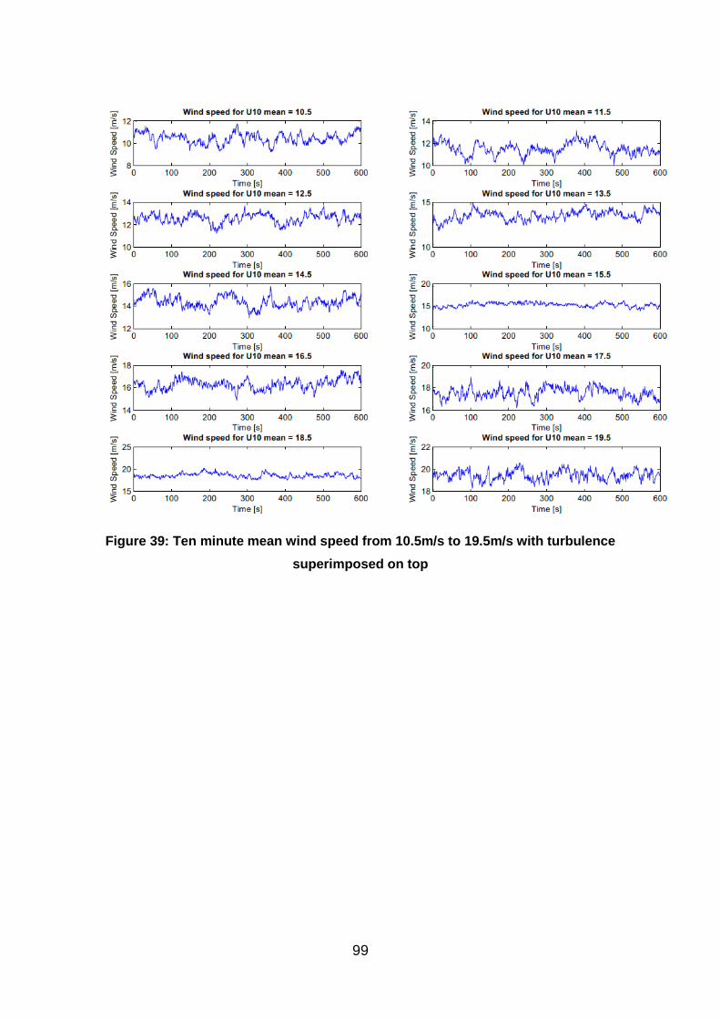
99
Figure 39: Ten minute mean wind speed from 10.5m/s to 19.5m/s with turbulence
superimposed on top
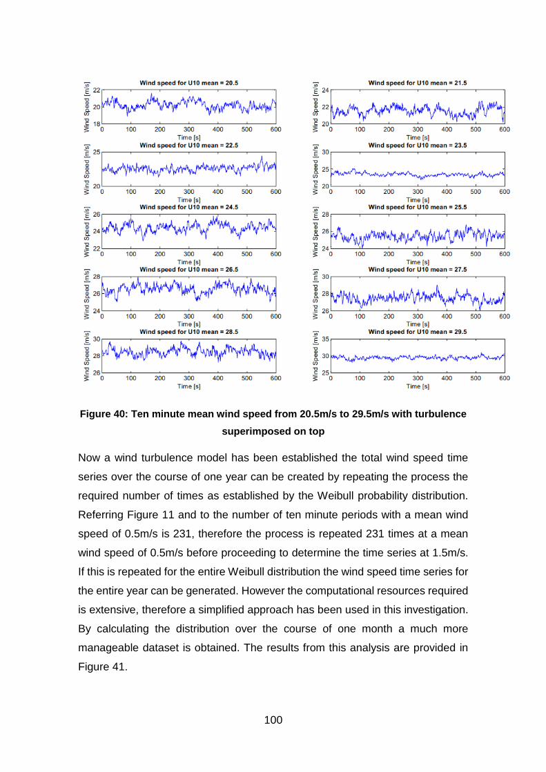
100
Figure 40: Ten minute mean wind speed from 20.5m/s to 29.5m/s with turbulence
superimposed on top
Now a wind turbulence model has been established the total wind speed time
series over the course of one year can be created by repeating the process the
required number of times as established by the Weibull probability distribution.
Referring Figure 11 and to the number of ten minute periods with a mean wind
speed of 0.5m/s is 231, therefore the process is repeated 231 times at a mean
wind speed of 0.5m/s before proceeding to determine the time series at 1.5m/s.
If this is repeated for the entire Weibull distribution the wind speed time series for
the entire year can be generated. However the computational resources required
is extensive, therefore a simplified approach has been used in this investigation.
By calculating the distribution over the course of one month a much more
manageable dataset is obtained. The results from this analysis are provided in
Figure 41.
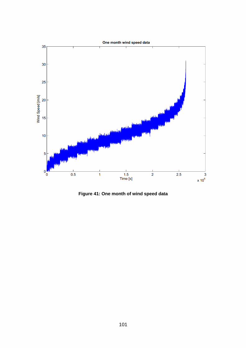
101
Figure 41: One month of wind speed data
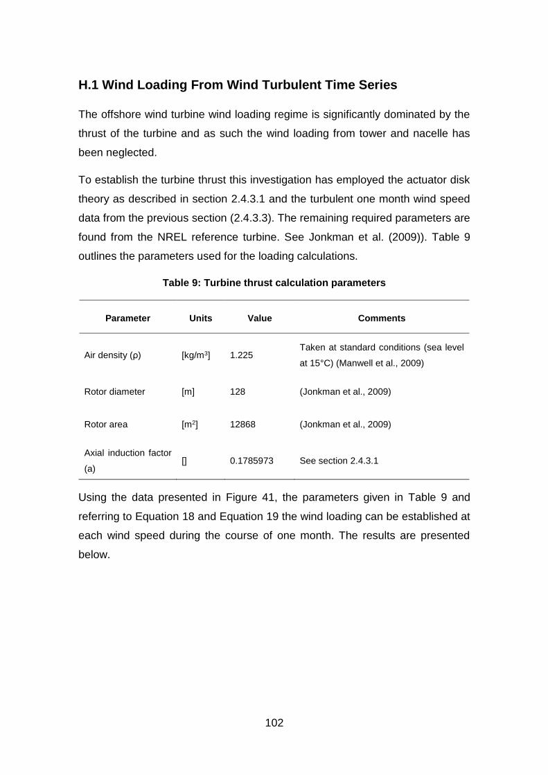
102
H.1 Wind Loading From Wind Turbulent Time Series
The offshore wind turbine wind loading regime is significantly dominated by the
thrust of the turbine and as such the wind loading from tower and nacelle has
been neglected.
To establish the turbine thrust this investigation has employed the actuator disk
theory as described in section 2.4.3.1 and the turbulent one month wind speed
data from the previous section (2.4.3.3). The remaining required parameters are
found from the NREL reference turbine. See Jonkman et al. (2009)). Table 9
outlines the parameters used for the loading calculations.
Table 9: Turbine thrust calculation parameters
Parameter Units Value Comments
Air density (ρ) [kg/m3] 1.225 Taken at standard conditions (sea level
at 15°C) (Manwell et al., 2009)
Rotor diameter [m] 128 (Jonkman et al., 2009)
Rotor area [m2] 12868 (Jonkman et al., 2009)
Axial induction factor
(a) [] 0.1785973 See section 2.4.3.1
Using the data presented in Figure 41, the parameters given in Table 9 and
referring to Equation 18 and Equation 19 the wind loading can be established at
each wind speed during the course of one month. The results are presented
below.
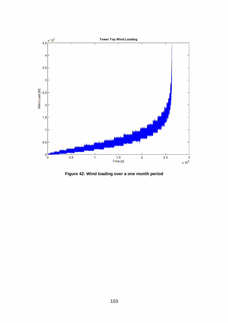
103
Figure 42: Wind loading over a one month period
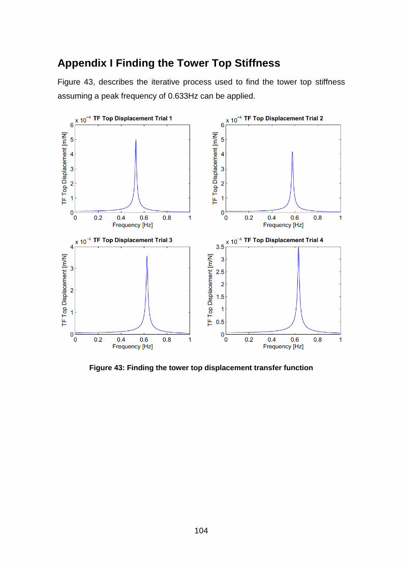
104
Appendix I Finding the Tower Top Stiffness
Figure 43, describes the iterative process used to find the tower top stiffness
assuming a peak frequency of 0.633Hz can be applied.
Figure 43: Finding the tower top displacement transfer function
105
Appendix J Finding the MWL Stiffness
The deflection of the structure can be established using the Double-Integration
method (Pytel and Kiusalaas, 2011) which yields a deflection equation at any
height, which in this case is the height anywhere along the turbine tower (see
Pytel and Kiusalaas (2011) for the full derivation and method explanation).
Equation 48 demonstrates the equation of the elastic curve used to establish the
deflection at the mean water level.
𝑑2𝛿
𝑑𝑧2=
𝑀
𝐸𝐼
Equation 48: Differential equation of the
elastic curve
𝑀 = 𝐹 × 𝑧 Equation 49: Moment
Where:
𝛿 = Deflection
𝑧 = Vertical distance up the turbine tower (z=0 at the mudline)
𝑀 = Moment
𝐹 = Force
𝐸 = Young’s modulus (210GPa from Jonkman et al. (2009))
𝐼 = 2nd moment of inertia
Given that the stiffness is now known at the top of the turbine where z=length,
the stiffness at the point where z=20 (MWL) can be established using the
following procedure.
𝐸𝐼𝛿 = ∬ 𝑀 𝑑𝑧 𝑑𝑧 + 𝐶1 + 𝐶2
𝐸𝐼𝛿 = ∬ 𝐹(ℎ − 𝑧) 𝑑𝑧 𝑑𝑧 + 𝐶1 + 𝐶2
Equation 50: Equation of the elastic
curve
Where:
106
ℎ = Height of the turbine (90m above the MWL and 20m below = 110m)
Preform the integration:
𝐸𝐼𝑑𝛿
𝑑𝑧= ∫ 𝐹(ℎ − 𝑧)𝑑𝑧
𝑧
0
𝐸𝐼𝑑𝛿
𝑑𝑧= ∫ (𝐹ℎ − 𝐹𝑧) 𝑑𝑧
𝑧
0
𝐸𝐼𝑑𝛿
𝑑𝑧= 𝐹ℎ𝑧 − 𝐹
𝑧2
2
𝐸𝐼𝛿 = ∫ 𝐹ℎ𝑧 − 𝐹𝑧2
2𝑑𝑧
𝑧
0
𝐸𝐼𝛿 = 𝐹ℎ𝑧2
2− 𝐹
𝑧3
6
Equation 51: Differential equation of the
elastic curve
Now take the situation where z=h:
𝐸𝐼𝛿 =𝐹ℎ3
2−
𝐹ℎ3
6
= 𝐹ℎ3 (1
2−
1
6)
𝐸𝐼𝛿 =𝐹ℎ3
3
Equation 52: Simplified equation of the
elastic curve where z=h
By equating Equation 52 with the equation for stiffness (force over deflection) a
new equation for stiffness is obtained as a function of height up the structure:
𝑘 =𝐹
𝛿=
3𝐸𝐼
ℎ3
Equation 53: Stiffness
Where:
𝑘 = Stiffness
107
𝛿 = Deflection
Now two equations can be presented, one for the known case where the stiffness
(k1) is equal to 143200N/m (see Table 5) and one for (k2) at the MWL where the
stiffness is unknown.
𝑘1 =3𝐸𝐼
ℎ13 = 143200N/m
Equation 54: Stiffness at hub height
𝑘2 =3𝐸𝐼
ℎ23
Equation 55: Stiffness at the MWL (1)
Where:
ℎ1 = Hub height from the seabed (110m)
ℎ2 = MWL (20m from seabed)
Assuming a constant value of I across the tower the following equation can be
used to find the stiffness at the MWL:
𝑘2 = 𝑘1 ×ℎ1
3
ℎ23
= 143200 ×1103
203
= 𝟐𝟑𝟖𝟐𝟒𝟗𝟎𝟎𝑵/𝒎
Equation 56: Stiffness at the MWL (2)
Finally the transfer function can be established for the wave loading using the
stiffness estimated at the MWL.
108
Appendix K Mudline Wind Bending Stress Transfer
Function
The following procedure is carried out using the flexure formula (Equation 57) to
find translate the displacement transfer function into a stress transfer function:
𝜎 =𝑀𝑦
𝐼
Equation 57: Flexure Formula (1) (Gere and
Goodno, 2009)
Which can be re-written in terms of the loading:
𝜎 =𝐹 × 𝐿 × 𝑦
𝐼 Equation 58: Flexure Formula (2)
And from Equation 53 it was found that:
𝛿 =𝐹ℎ3
3𝐸𝐼
Equation 59: Deflection as a function of
height
Thus by equating Equation 58 and Equation 59 the following relationship is
established:
𝜎 = 𝛿 × [3𝐸𝑦
𝐿2]
Equation 60: Bending stress in terms of
displacement
Where:
𝜎 = Bending stress [Pa]
𝐼 = 2nd Moment of inertia of the cross-sectional area [m4] (assumed constant
across entire structure)
𝑀 = Bending moment [Nm]
𝐸 = Young’s modulus (210GPa from Jonkman et al. (2009))
𝐹 = Force [N]
𝐿 = Length [m] (110m from hub to mudline)
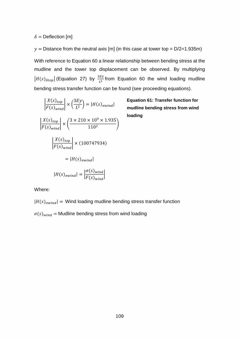
109
𝛿 = Deflection [m]
𝑦 = Distance from the neutral axis [m] (in this case at tower top = D/2=1.935m)
With reference to Equation 60 a linear relationship between bending stress at the
mudline and the tower top displacement can be observed. By multiplying
|𝐻(𝑠)𝛿𝑡𝑜𝑝| (Equation 27) by 3𝐸𝑦
𝐿2 from Equation 60 the wind loading mudline
bending stress transfer function can be found (see proceeding equations).
|𝑋(𝑠)𝑡𝑜𝑝
𝐹(𝑠)𝑤𝑖𝑛𝑑| × (
3𝐸𝑦
𝐿2) = |𝐻(𝑠)𝜎𝑤𝑖𝑛𝑑|
|𝑋(𝑠)𝑡𝑜𝑝
𝐹(𝑠)𝑤𝑖𝑛𝑑| × (
3 × 210 × 109 × 1.935
1102)
|𝑋(𝑠)𝑡𝑜𝑝
𝐹(𝑠)𝑤𝑖𝑛𝑑| × (100747934)
= |𝐻(𝑠)𝜎𝑤𝑖𝑛𝑑|
|𝐻(𝑠)𝜎𝑤𝑖𝑛𝑑| = |𝜎(𝑠)𝑤𝑖𝑛𝑑
𝐹(𝑠)𝑤𝑖𝑛𝑑|
Equation 61: Transfer function for
mudline bending stress from wind
loading
Where:
|𝐻(𝑠)𝜎𝑤𝑖𝑛𝑑| = Wind loading mudline bending stress transfer function
𝜎(𝑠)𝑤𝑖𝑛𝑑 = Mudline bending stress from wind loading
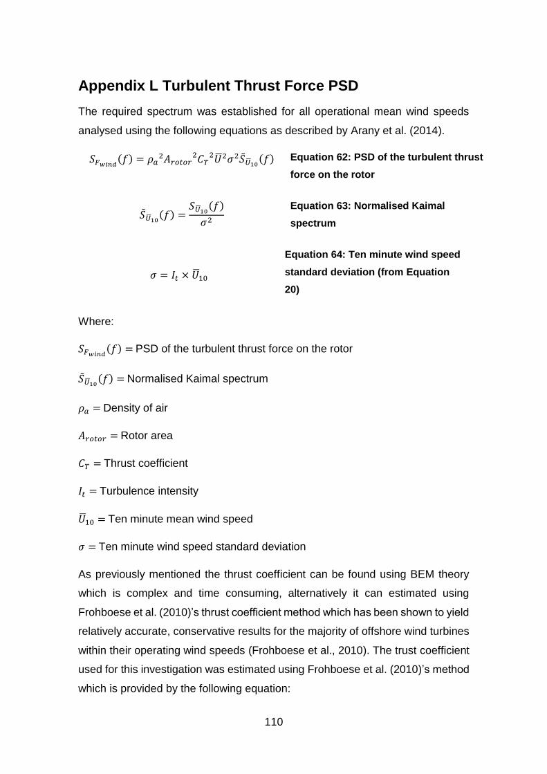
110
Appendix L Turbulent Thrust Force PSD
The required spectrum was established for all operational mean wind speeds
analysed using the following equations as described by Arany et al. (2014).
𝑆𝐹𝑤𝑖𝑛𝑑(𝑓) = 𝜌𝑎
2𝐴𝑟𝑜𝑡𝑜𝑟2𝐶𝑇
2�̅�2𝜎2�̃��̅�10(𝑓) Equation 62: PSD of the turbulent thrust
force on the rotor
�̃��̅�10(𝑓) =
𝑆�̅�10(𝑓)
𝜎2
Equation 63: Normalised Kaimal
spectrum
𝜎 = 𝐼𝑡 × �̅�10
Equation 64: Ten minute wind speed
standard deviation (from Equation
20)
Where:
𝑆𝐹𝑤𝑖𝑛𝑑(𝑓) = PSD of the turbulent thrust force on the rotor
�̃��̅�10(𝑓) = Normalised Kaimal spectrum
𝜌𝑎 = Density of air
𝐴𝑟𝑜𝑡𝑜𝑟 = Rotor area
𝐶𝑇 = Thrust coefficient
𝐼𝑡 = Turbulence intensity
�̅�10 = Ten minute mean wind speed
𝜎 = Ten minute wind speed standard deviation
As previously mentioned the thrust coefficient can be found using BEM theory
which is complex and time consuming, alternatively it can estimated using
Frohboese et al. (2010)’s thrust coefficient method which has been shown to yield
relatively accurate, conservative results for the majority of offshore wind turbines
within their operating wind speeds (Frohboese et al., 2010). The trust coefficient
used for this investigation was estimated using Frohboese et al. (2010)’s method
which is provided by the following equation:
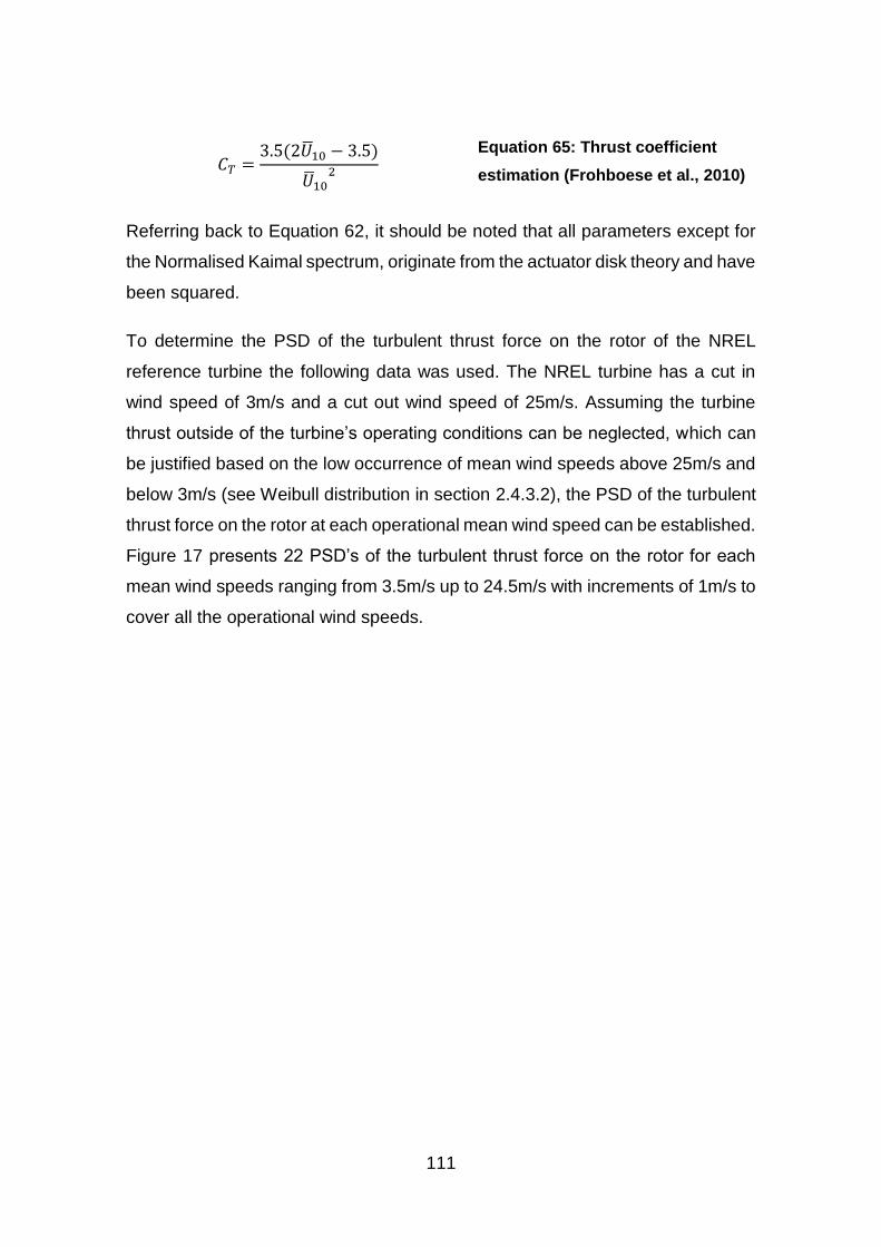
111
𝐶𝑇 =3.5(2�̅�10 − 3.5)
�̅�102
Equation 65: Thrust coefficient
estimation (Frohboese et al., 2010)
Referring back to Equation 62, it should be noted that all parameters except for
the Normalised Kaimal spectrum, originate from the actuator disk theory and have
been squared.
To determine the PSD of the turbulent thrust force on the rotor of the NREL
reference turbine the following data was used. The NREL turbine has a cut in
wind speed of 3m/s and a cut out wind speed of 25m/s. Assuming the turbine
thrust outside of the turbine’s operating conditions can be neglected, which can
be justified based on the low occurrence of mean wind speeds above 25m/s and
below 3m/s (see Weibull distribution in section 2.4.3.2), the PSD of the turbulent
thrust force on the rotor at each operational mean wind speed can be established.
Figure 17 presents 22 PSD’s of the turbulent thrust force on the rotor for each
mean wind speeds ranging from 3.5m/s up to 24.5m/s with increments of 1m/s to
cover all the operational wind speeds.
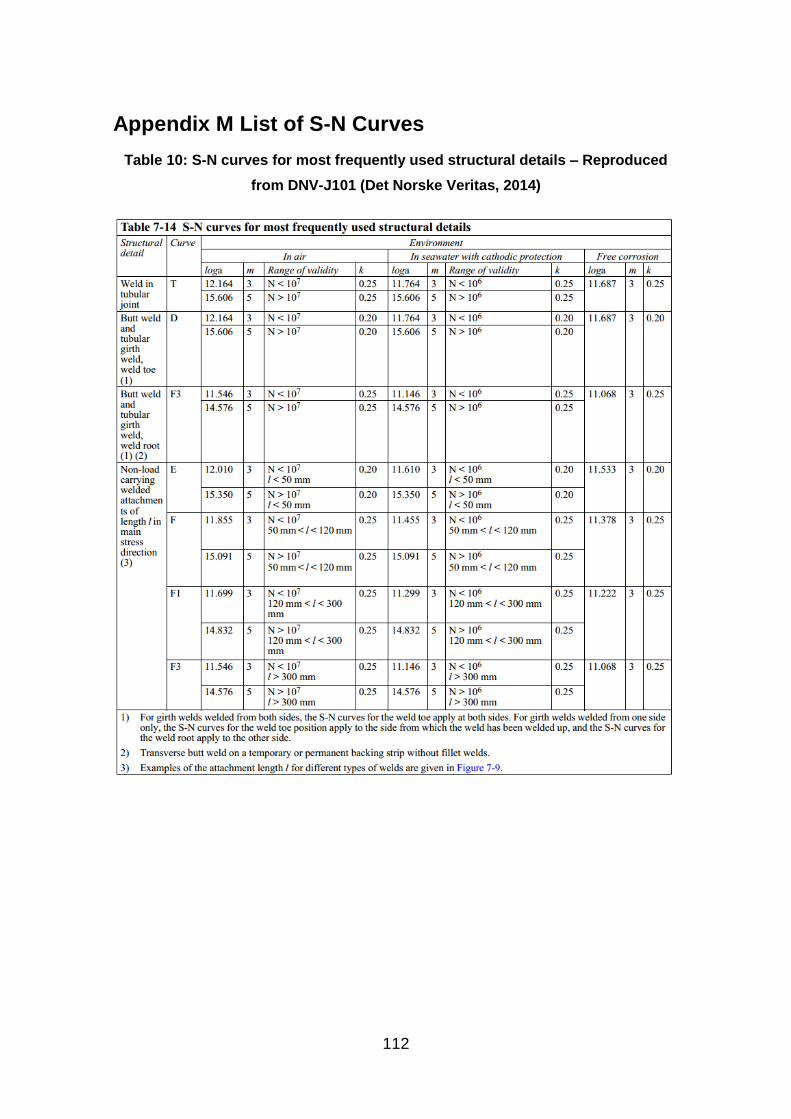
112
Appendix M List of S-N Curves
Table 10: S-N curves for most frequently used structural details – Reproduced
from DNV-J101 (Det Norske Veritas, 2014)
Recommended