MICRO-LEVEL ESTIMATION OF POVERTY AND INEQUALITY
By Chris Elbers, Jean O. Lanjouw, and Peter Lanjouw1
1. Introduction
Recent theoretical advances have brought income and wealth distributions back
into a prominent position in growth and development theories, and as determinants of
speci¯c socio-economic outcomes, such as health or levels of violence. Empirical investi-
gation of the importance of these relationships, however, has been held back by the lack
of su±ciently detailed high quality data on distributions. Household surveys that include
reasonable measures of income or consumption can be used to calculate distributional
measures but at low levels of aggregation these samples are rarely representative or of
su±cient size to yield statistically reliable estimates. At the same time, census (or other
large sample) data of su±cient size to allow disaggregation either have no information
about income or consumption, or measure these variables poorly. This note outlines a
statistical procedure to combine these types of data to take advantage of the detail in
household sample surveys and the comprehensive coverage of a census. It extends the
literature on small area statistics (Ghosh and Rao (1994), Rao (1999)) by developing esti-
mators of population parameters which are non-linear functions of the underlying variable
1
of interest (here unit level consumption), and by deriving them from the full unit level
distribution of that variable.
In examples using Ecuadorian data, our estimates have levels of precision compara-
ble to those of commonly used survey based welfare estimates - but for populations as
small as 15,000 households, a `town'. This is an enormous improvement over survey
based estimates, which are typically only consistent for areas encompassing hundreds of
thousands, even millions, of households. Experience using the method in South Africa,
Brazil, Panama, Madagascar and Nicaragua suggest that Ecuador is not an unusual case
(Alderman, et. al. (2002), and Elbers, Lanjouw, Lanjouw, and Leite (2002)).
2. The Basic Idea
The idea is straightforward. Let W be an indicator of poverty or inequality based
on the distribution of a household-level variable of interest, yh. Using the smaller and
richer data sample, we estimate the joint distribution of yh and a vector of covariates,
xh: By restricting the set of explanatory variables to those that can also be linked to
households in the larger sample or census, this estimated distribution can be used to
generate the distribution of yh for any sub-population in the larger sample conditional on
the sub-population's observed characteristics. This, in turn, allows us to generate the
conditional distribution of W , in particular, its point estimate and prediction error.
2
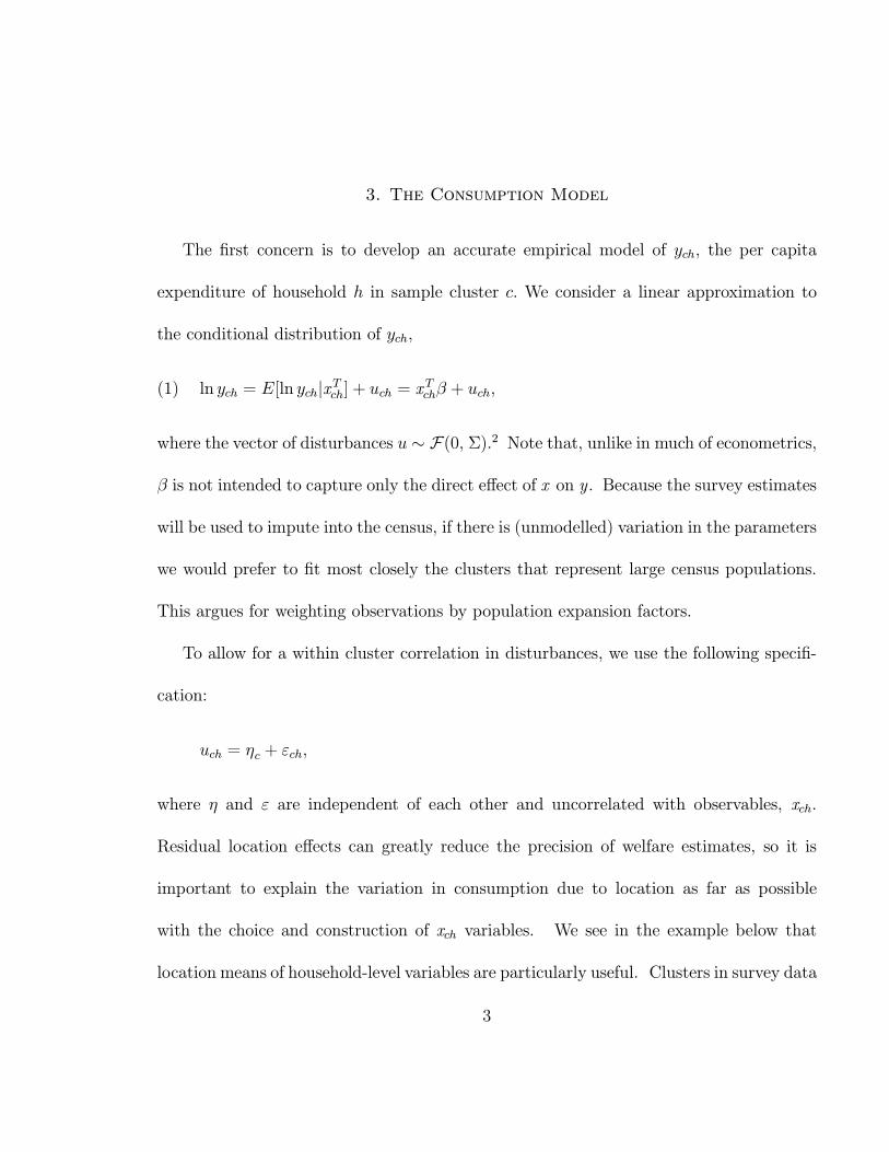
3. The Consumption Model
The ¯rst concern is to develop an accurate empirical model of ych; the per capita
expenditure of household h in sample cluster c: We consider a linear approximation to
the conditional distribution of ych;
ln ych = E[ln ychjxTch] + uch = xTch¯ + uch;(1)
where the vector of disturbances u » F(0, §):2 Note that, unlike in much of econometrics,
¯ is not intended to capture only the direct e®ect of x on y : Because the survey estimates
will be used to impute into the census, if there is (unmodelled) variation in the parameters
we would prefer to ¯t most closely the clusters that represent large census populations.
This argues for weighting observations by population expansion factors.
To allow for a within cluster correlation in disturbances, we use the following speci¯-
cation:
uch = ´c + "ch;
where ´ and " are independent of each other and uncorrelated with observables, xch:
Residual location e®ects can greatly reduce the precision of welfare estimates, so it is
important to explain the variation in consumption due to location as far as possible
with the choice and construction of xch variables. We see in the example below that
location means of household-level variables are particularly useful. Clusters in survey data
3
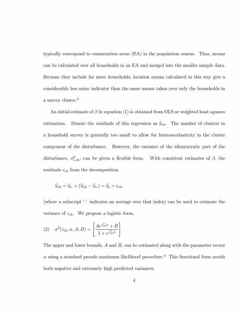
typically correspond to enumeration areas (EA) in the population census. Thus, means
can be calculated over all households in an EA and merged into the smaller sample data.
Because they include far more households, location means calculated in this way give a
considerably less noisy indicator than the same means taken over only the households in
a survey cluster.3
An initial estimate of ¯ in equation (1) is obtained from OLS or weighted least squares
estimation. Denote the residuals of this regression as buch: The number of clusters ina household survey is generally too small to allow for heteroscedasticity in the cluster
component of the disturbance. However, the variance of the idiosyncratic part of the
disturbance, ¾2";ch; can be given a °exible form. With consistent estimates of ¯, the
residuals ech from the decomposition
buch = buc: + (buch ¡ buc:) = b́c + ech;(where a subscript `.' indicates an average over that index) can be used to estimate the
variance of "ch. We propose a logistic form,
¾2(zch; ®; A;B) =
"Aez
Tch® +B
1 + ezTch®
#:(2)
The upper and lower bounds, A and B, can be estimated along with the parameter vector
® using a standard pseudo maximum likelihood procedure.4 This functional form avoids
both negative and extremely high predicted variances.
4
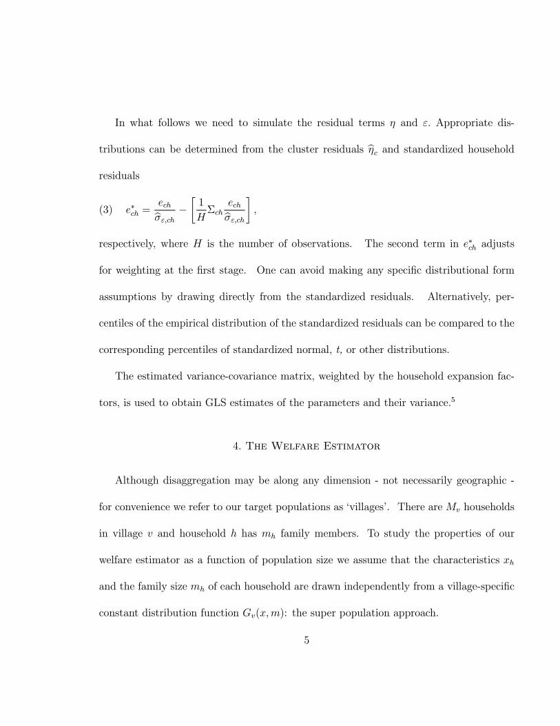
In what follows we need to simulate the residual terms ´ and ": Appropriate dis-
tributions can be determined from the cluster residuals b́c and standardized householdresiduals
e¤ch =echb¾";ch ¡
·1
H§ch
echb¾";ch¸;(3)
respectively, where H is the number of observations. The second term in e¤ch adjusts
for weighting at the ¯rst stage. One can avoid making any speci¯c distributional form
assumptions by drawing directly from the standardized residuals. Alternatively, per-
centiles of the empirical distribution of the standardized residuals can be compared to the
corresponding percentiles of standardized normal, t, or other distributions.
The estimated variance-covariance matrix; weighted by the household expansion fac-
tors, is used to obtain GLS estimates of the parameters and their variance.5
4. The Welfare Estimator
Although disaggregation may be along any dimension - not necessarily geographic -
for convenience we refer to our target populations as `villages'. There areMv households
in village v and household h has mh family members. To study the properties of our
welfare estimator as a function of population size we assume that the characteristics xh
and the family size mh of each household are drawn independently from a village-speci¯c
constant distribution function Gv(x;m): the super population approach.
5
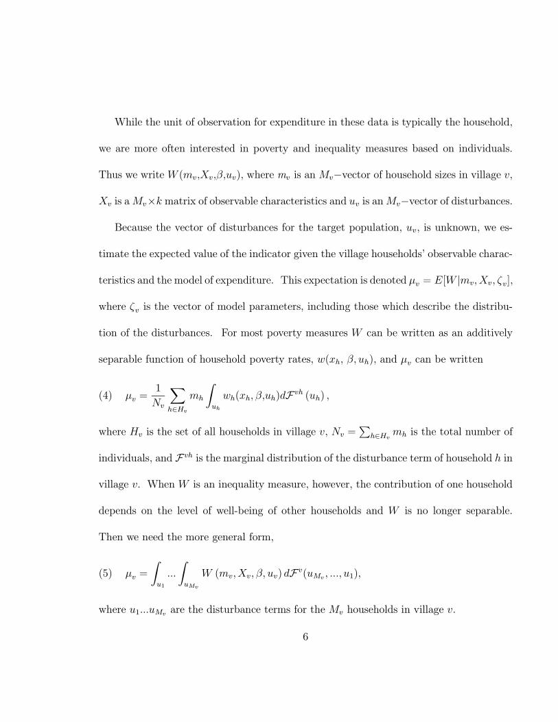
While the unit of observation for expenditure in these data is typically the household,
we are more often interested in poverty and inequality measures based on individuals.
Thus we write W (mv;Xv;¯;uv); where mv is an Mv¡vector of household sizes in village v;
Xv is aMv£k matrix of observable characteristics and uv is anMv¡vector of disturbances.
Because the vector of disturbances for the target population, uv, is unknown, we es-
timate the expected value of the indicator given the village households' observable charac-
teristics and the model of expenditure. This expectation is denoted ¹v = E[W jmv; Xv; ³v];
where ³v is the vector of model parameters, including those which describe the distribu-
tion of the disturbances. For most poverty measures W can be written as an additively
separable function of household poverty rates, w(xh, ¯; uh); and ¹v can be written
¹v =1
Nv
Xh2Hv
mh
Zuh
wh(xh; ¯;uh)dFvh (uh) ;(4)
where Hv is the set of all households in village v, Nv =P
h2Hv mh is the total number of
individuals, and Fvh is the marginal distribution of the disturbance term of household h in
village v: When W is an inequality measure, however, the contribution of one household
depends on the level of well-being of other households and W is no longer separable.
Then we need the more general form,
¹v =
Zu1
:::
ZuMv
W (mv;Xv; ¯; uv) dFv(uMv ; :::; u1);(5)
where u1:::uMv are the disturbance terms for the Mv households in village v:
6
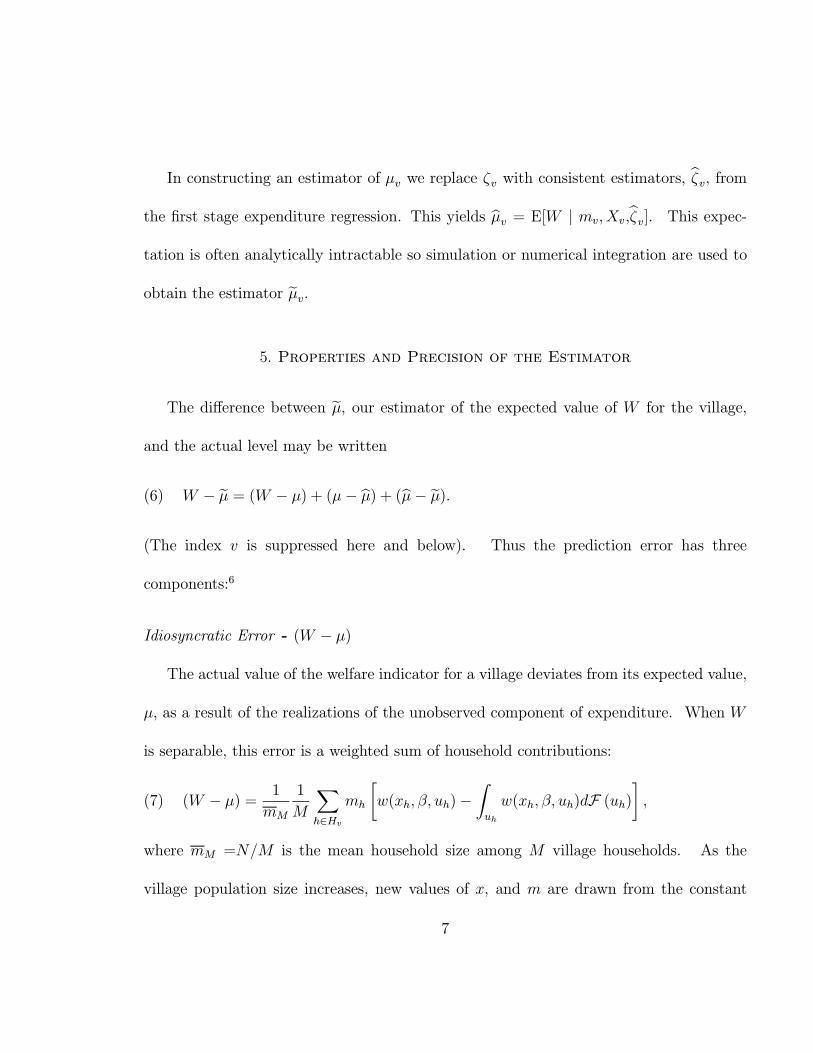
In constructing an estimator of ¹v we replace ³v with consistent estimators, b³v, fromthe ¯rst stage expenditure regression. This yields b¹v = E[W j mv; Xv;b³v]. This expec-
tation is often analytically intractable so simulation or numerical integration are used to
obtain the estimator e¹v:5. Properties and Precision of the Estimator
The di®erence between e¹, our estimator of the expected value of W for the village,
and the actual level may be written
W ¡ e¹ = (W ¡ ¹) + (¹¡ b¹) + (b¹¡ e¹):(6)
(The index v is suppressed here and below). Thus the prediction error has three
components:6
Idiosyncratic Error - (W ¡ ¹)
The actual value of the welfare indicator for a village deviates from its expected value,
¹, as a result of the realizations of the unobserved component of expenditure. When W
is separable, this error is a weighted sum of household contributions:
(W ¡ ¹) = 1
mM
1
M
Xh2Hv
mh
·w(xh; ¯; uh)¡
Zuh
w(xh; ¯; uh)dF (uh)¸;(7)
where mM =N/M is the mean household size among M village households. As the
village population size increases, new values of x, and m are drawn from the constant
7
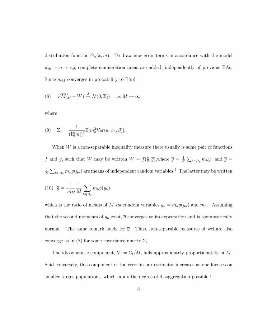
distribution function Gv(x;m): To draw new error terms in accordance with the model
uch = ´c + "ch complete enumeration areas are added, independently of previous EAs.
Since mM converges in probability to E[m],
pM(¹¡W ) d! N (0;§I) as M !1;(8)
where
§I =1
(E[m])2E[m2
hVar(wjxh; ¯)].(9)
When W is a non-separable inequality measure there usually is some pair of functions
f and g; such that W may be written W = f(y; g);where y = 1N
Ph2Hv mhyh and g =
1N
Ph2Hv mhg(yh) are means of independent random variables.
7 The latter may be written
g =1
mM
1
M
Xh2Hv
mhg(yh);(10)
which is the ratio of means of M iid random variables gh = mhg(yh) and mh. Assuming
that the second moments of gh exist, g converges to its expectation and is asymptotically
normal. The same remark holds for y: Thus, non-separable measures of welfare also
converge as in (8) for some covariance matrix §I.
The idiosyncratic component, VI = §I=M; falls approximately proportionately in M .
Said conversely, this component of the error in our estimator increases as one focuses on
smaller target populations, which limits the degree of disaggregation possible.8
8
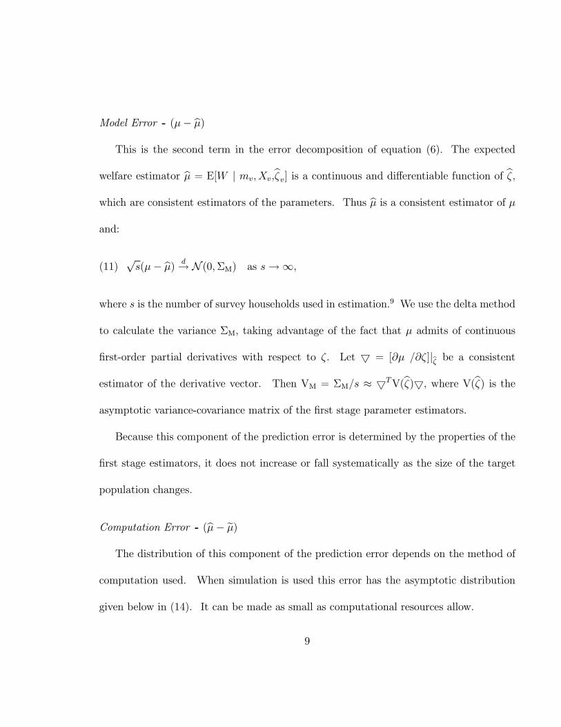
Model Error - (¹¡ b¹)This is the second term in the error decomposition of equation (6). The expected
welfare estimator b¹ = E[W j mv; Xv;b³v] is a continuous and di®erentiable function of b³,which are consistent estimators of the parameters. Thus b¹ is a consistent estimator of ¹and:
ps(¹¡ b¹) d!N (0;§M) as s!1;(11)
where s is the number of survey households used in estimation.9 We use the delta method
to calculate the variance §M; taking advantage of the fact that ¹ admits of continuous
¯rst-order partial derivatives with respect to ³: Let 5 = [@¹ /@³ ]jb³ be a consistentestimator of the derivative vector. Then VM = §M/s ¼ 5TV(b³)5, where V(b³) is theasymptotic variance-covariance matrix of the ¯rst stage parameter estimators.
Because this component of the prediction error is determined by the properties of the
¯rst stage estimators, it does not increase or fall systematically as the size of the target
population changes.
Computation Error - (b¹¡ e¹)The distribution of this component of the prediction error depends on the method of
computation used. When simulation is used this error has the asymptotic distribution
given below in (14). It can be made as small as computational resources allow.
9
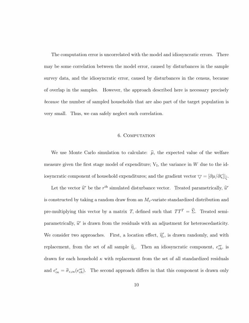
The computation error is uncorrelated with the model and idiosyncratic errors. There
may be some correlation between the model error, caused by disturbances in the sample
survey data, and the idiosyncratic error, caused by disturbances in the census, because
of overlap in the samples. However, the approach described here is necessary precisely
because the number of sampled households that are also part of the target population is
very small. Thus, we can safely neglect such correlation.
6. Computation
We use Monte Carlo simulation to calculate: b¹, the expected value of the welfaremeasure given the ¯rst stage model of expenditure; VI, the variance in W due to the id-
iosyncratic component of household expenditures; and the gradient vector 5 = [@¹/@³]jb³.Let the vector bur be the rth simulated disturbance vector. Treated parametrically, bur
is constructed by taking a random draw from anMv-variate standardized distribution and
pre-multiplying this vector by a matrix T, de¯ned such that TT T = b§: Treated semi-parametrically, bur is drawn from the residuals with an adjustment for heteroscedasticity.
We consider two approaches. First, a location e®ect, b́rc; is drawn randomly, and withreplacement, from the set of all sample b́c: Then an idiosyncratic component, e¤rch; is
drawn for each household · with replacement from the set of all standardized residuals
and erc· = b¾";c·(e¤rch). The second approach di®ers in that this component is drawn only10
from the standardized residuals e¤ch that correspond to the cluster from which household
·'s location e®ect was derived. Although b́c and ech are uncorrelated, the second approachallows for non-linear relationships between location and household unobservables.
With each vector of simulated disturbances we construct a value for the indicator,
cWr = W (m;bt; bur); where bt = Xb̄, the predicted part of log per-capita expenditure. Thesimulated expected value for the indicator is the mean over R replications,
e¹ = 1
R
RXr=1
cWr:(12)
The variance of W around its expected value ¹ due to the idiosyncratic component
of expenditures can be estimated in a straightforward manner using the same simulated
values,
eVI = 1
R
RXr=1
(cWr ¡ e¹)2:(13)
Simulated numerical gradient estimators are constructed as follows: We make a positive
perturbation to a parameter estimate, say b̄k, by adding ±jb̄kj, and then calculate bt+;followed by cW+
r = W (m;bt+; bur), and e¹+. A negative perturbation of the same size is
used to obtain e¹¡. The simulated central distance estimator of the derivative @¹=@¯kjb³ is(e¹+¡ e¹¡)=(2±jb̄kj): As we use the same simulation draws in the calculation of e¹, e¹+ande¹¡, these gradient estimators are consistent as long as ± is speci¯ed to fall su±cientlyrapidly as R ! 1 (Pakes and Pollard (1989)). Having thus derived an estimate of the
11
gradient vector 5 = [@¹=@³]jb³ , we can calculate eVM = 5TV(b³)5.Because e¹ is a sample mean of R independent random draws from the distribution of
(W jm;bt; b§), the central limit theorem implies that
pR(e¹¡ b¹) d!N (0;§C) as R!1;(14)
where §C =Var(W jm;bt; b§):When the decomposition of the prediction error into its component parts is not im-
portant, a far more e±cient computational strategy is available. Write
ln ych = xTch¯ + ´c(³) + "ch(³);
where we have stressed that the distribution of ´ and " depend on the parameter vector
³. By simulating ³ from the sampling distribution of b³, and f´rcg and f"rchg conditionalon the simulated value ³r, we obtain simulated values fyrchg, consistent with the model's
distributional characteristics, from which welfare estimates W r can be derived (Mackay
(1998)). Estimates of expected welfare, ¹, and its variance are calculated as in equations
(12) and (13). Drawing from the sampling distribution of the parameters replaces the
delta method as a way to incorporate model error into the total prediction error. Equation
(13) now gives a sum of the variance components eVI + eVM; while §C in equation (14)becomes §C =Var(W jm;X;b³;V(b³)):
12
7. Results
We apply the approach using household per capita expenditure as our measure of
well-being, yh; but others could be used, such as assets, income, or health status. Our
smaller detailed sample is the 1994 Ecuadorian Encuesta Sobre Las Condiciones de Vida,
a household survey following the general format of a World Bank Living Standards Mea-
surement Survey. It is strati¯ed by 8 regions and is representative only at that level.
Our larger sample is the 1990 Ecuadorian census.
Models are estimated for each stratum. Hausman tests indicate that expansion factors
have a statistically signi¯cant e®ect on our coe±cients, so we weight accordingly (see
Deaton (1997)). Subsequent analysis of the resulting estimates of welfare for localities
in rural Costa indicates that this choice has a substantial e®ect on estimated welfare
rankings. (See Elbers, Lanjouw, and Lanjouw (2002) for a fuller discussion of all results.)
Most of the e®ect of location on consumption is captured with available explanatory
variables. In the rural Costa stratum, for example, the estimated share of the location
component in the total residual variance, b¾2´=b¾2u; falls from 14% to 5% with the inclusion
of location means (but no infrastructure variables) and to just 2% with the addition of
information about household access to sewage infrastructure.10 Using the latter model,
in that stratum we cannot reject the null hypothesis that location e®ects are jointly zero
in a ¯xed e®ects speci¯cation.
13
Heteroscedasticity models are selected from all potential explanatory variables, their
squares, cubes and interactions.11 In all strata, chi-square tests of the null that estimated
parameters are jointly zero reject homoscedasticity (with p-values < 0.001). As with
weighting, subsequent analysis for rural Costa indicates that allowing this °exibility has
a substantial e®ect on estimated welfare rankings of localities.
For some strata in Ecuador the standarized residual distribution appears to be ap-
proximately normal, even if formally rejected by tests based on skewness and kurtosis.
Elsewhere, we ¯nd a t(5) distribution to be the better approximation. Relaxing the
distributional form restrictions on the disturbance term and taking either of the semi-
parametric approaches outlined above makes very little di®erence in the results for our
Ecuadorian example.
Simulation results for the headcount measure of poverty and the general entropy (0.5)
measure of inequality are in Table I. (For other measures see Elbers, et. al. (2002).) We
construct populations of increasing size from a constant distribution Gv(x;m) by drawing
households randomly from all census households in the rural Costa region. They are
allocated in groups of 100 to pseudo enumeration areas, with `parroquias' of a thousand
households created out of groups of ten EAs. We continue aggregating to obtain nested
populations with 100 to 100,000 households. For each population, the table shows esti-
mates of the expected value of the welfare indicator, the standard error of the prediction,
14
and the share of the total variance due to the idiosyncratic component. The location
e®ect estimated at the cluster level in the survey data is applied to EAs in the census.
In all cases the standard error due to computation is less than 0.001.
Looking across columns one sees how the variance of the estimator falls as the size
of the target population increases. For both measures the total standard error of the
prediction falls to about ¯ve percent of the point estimate with a population of just
15,000 households. At this point, the share of the total variance due to the idiosyncratic
component of expenditure is already small, so there is little to gain from moving to higher
levels of aggregation. The table also shows that estimates for populations of 100 have
large errors Clearly it would be ill advised to use this approach to determine the poverty
of yet smaller groups or single households.
Most users of welfare indicators rely, by necessity, on sample survey based estimates.
Table II demonstrates how much is gained by combining data sources. The second column
gives the sampling errors on headcount measures estimated for each stratum using the
survey data alone (taking account of sample design). There is only one estimate per
region as this is the lowest level at which the sample is representative. The population of
each region is in the third column. When combining census and survey data it becomes
possible to disaggregate to sub-regions and estimate poverty for speci¯c localities. Here we
choose as sub-regions parroquias or, in the cities of Quito and Guayaquil, zonas, because
15
our prediction errors for these administrative units are similar in magnitude to the survey
based sampling error on the region level estimates. (See the median standard error among
sub-regions in the fourth column.) The ¯nal column gives the median population among
these sub-regions. Comparing the third and ¯nal columns it is clear that, for the same
prediction error commonly encountered in sample data, one can estimate poverty using
combined data for sub-populations of a hundredth the size. This becomes increasingly
useful the more there is spatial variation in well-being that can be identi¯ed using this
approach. Considering this question, Demombynes, et. al. (2002) ¯nd, for several
countries, that most sub-region headcount estimates do di®er signi¯cantly from their
region's average level.
We can also answer questions about the level and heterogeneity of welfare at di®erent
levels of governmental adminstration. Decomposing inequality in rural Ecuador into
between and within group components, we ¯nd that even at the level of parroquias 85% of
overall rural inequality can still be attributed to di®erences within groups. Thus, as often
suggested by anecdotal evidence, even within local communities there exists a considerable
heterogeneity of living standards. This may a®ect the likelihood of political capture
(Bardhan and Mookherjee (1999)), the functioning of local institutions, the feasibility of
raising revenues locally, and other issues of importance in political economy and public
policy. We expect that the empirical analysis of these issues will be strengthened by the
16
micro-level information on distribution that the method described here can o®er.
Department of Economics, Vrije Universiteit, De Boelelaan 1105, 1081 HV Amster-
dam, N.L.; [email protected],
and
Department of Economics, Yale University and the Brookings Institution, 1775 Mas-
sachusetts Avenue NW, Washington, DC, 20036, U.S.A.; [email protected],
and
The World Bank, 1818 H. Street, Washington, DC, 20433, U.S.A.; [email protected].
17
REFERENCES
Alderman, H., M. Babita, G. Demombynes, N. Makhatha, and B. ÄOzler
(2002): \How Low Can You Go?: Combining Census and Survey Data for Mapping
Poverty in South Africa," Journal of African Economics, forthcoming.
Bardhan, P., and D. Mookherjee (1999): \Relative Capture of Local and Central
Governments: An Essay in the Political Economy of Decentralization," CIDER
Working Paper no. C99-109, University of California at Berkeley.
Chesher, A., and C. Schluter (2002): \Welfare Measurement and Measurement
Error," Review of Economic Studies, forthcoming.
Deaton, A. (1997): The Analysis of Household Surveys: A Microeconometric Approach
to Development Policy. Washington, D.C.: The Johns Hopkins University Press for
the World Bank.
Demombynes, G., C. Elbers, J. O. Lanjouw, P. Lanjouw, J. Mistiaen, and
B. }Ozler (2002): \Producing an Improved Geographic Pro¯le of Poverty: Method-
ology and Evidence from Three Developing Countries," WIDER Discussion Paper
no. 2002/39, The United Nations.
18
Elbers, C., J. O. Lanjouw, and P. Lanjouw (2000): \Welfare in Villages and
Towns: Micro-Measurement of Poverty and Inequality," Tinbergen Institute Work-
ing Paper no. 2000-029/2.
(2002): \Micro-Level Estimation of Welfare," Policy Research Department Working
Paper, The World Bank, forthcoming.
Elbers, C., J. O. Lanjouw, P. Lanjouw, and P. G. Leite (2001): \Poverty and
Inequality in Brazil: New Estimates from Combined PPV-PNAD Data," Unpub-
lished Manuscript, The World Bank.
Ghosh, M., and J. N. K. Rao (1994): \Small Area Estimation: An Appraisal,"
Statistical Science, 9, 55-93.
Greene, W. H. (2000): Econometric Analysis. Fourth Edition. New Jersey: Prentice-
Hall Inc.
Keyzer, M., and Y. Ermoliev (2000): \Reweighting Survey Observations by Monte
Carlo Integration on a Census," Stichting Onderzoek Wereldvoedselvoorziening,
Sta® Working Paper no. 00.04, the Vrije Universiteit, Amsterdam.
Mackay, D. J. C. (1998): \Introduction to Monte Carlo Methods," in Learning in
Graphical Models; Proceedings of the NATO Advanced Study Institute, ed. by M. I.
19
Jordan. Kluwer Academic Publishers Group.
Pakes, A., and D. Pollard (1989): \Simulation and the Asymptotics of Optimiza-
tion Estimators," Econometrica, 57, 1027-58.
Rao, J. N. K. (1999): \Some Recent Advances in Model-Based Small Area Estimation,"
Survey Methodology, 25, 175-86.
Tarozzi, A. (2001): \Estimating Comparable Poverty Counts from Incomparable Sur-
veys: Measuring Poverty in India," Unpublished Manuscript, Princeton University.
20
FOOTNOTES
1 We are very grateful to Ecuador's Instituto Nacional de Estadistica y Censo (INEC)
for making its 1990 unit-record census data available to us. Much of this research was
done while the authors were at the Vrije Universiteit, Amsterdam, and we appreciate
the hospitality and input from colleagues there. We also thank Don Andrews, Fran»cois
Bourguignon, Andrew Chesher, Denis Cogneau, Angus Deaton, Jean-Yves Duclos, Fran-
cisco Ferreira, Jesko Hentschel, Michiel Keyzer, Steven Ludlow, Berk }Ozler, Giovanna
Prennushi, Martin Ravallion, Piet Rietveld, John Rust and Chris Udry for comments
and useful discussions, as well as seminar participants at the Vrije Universiteit, ENRA
(Paris), U.C. Berkeley, Georgetown University, the World Bank and the Brookings Insti-
tution. Financial support was received from the Bank Netherlands Partnership Program.
However, the views presented here should not be taken to re°ect those of the World Bank
or any of its a±liates. All errors are our own.
2 One could consider estimating E(yjx) or the conditional density p(yjx) non-parametrically.
In estimating expenditure for each household in the populations of interest (perhaps to-
talling millions) conditioning on, say, thirty observed characteristics, a major di±culty
is to ¯nd a method of weighting that lowers the computational burden. See Keyzer and
Ermoliev (2000) and Tarozzi (2001) for examples and discussion.
3 Other sources of information could be merged with both census and survey datasets
21
to explain location e®ects as needed. Geographic information system databases, for
example, allow a multitude of environmental and community characteristics to be geo-
graphically de¯ned both comprehensively and with great precision.
4 An estimate of the variance of the estimators can be derived from the information
matrix and used to construct a Wald test for homoscedasticity (Greene (2000), Section
12.5.3). Allowing the bounds to be freely estimated generates a standardized distribution
for predicted disturbances which is well behaved in our experience. This is particularly
important when using the standardized residuals directly in a semi-parametric approach to
simulation (see Section 6 below.) However, we have also found that imposing a minimum
bound of zero and a maximum bound A¤ = (1:05)maxfe2chg yields similar estimates of
the parameters ® . These restrictions allow one to estimate the simpler form lnh
e2chA¤¡e2ch
i= zTch®+ rch: Use of this form would be a practical approach for initial model selection.
5 In our experience, model estimates have been very robust to estimation strategy,
with weighted GLS estimates not signi¯cantly di®erent from the results of OLS or quantile
regressions weighted by expansion factors.
6 Our target is the level of welfare that could be calculated if we were fortunate
enough to have observations on expenditure for all households in a population. Clearly
because expenditures are measured with error this may di®er from a measure based on true
expenditures. See Chesher and Schluter (2002) for methods to estimate the sensitivity
22
of welfare measures to mismeasurement in y:
7 The Gini coe±cient is an exception but it can be handled e®ectively with a separable
approximation. See Elbers, et. al. (2000).
8 The above discussion concerns the asymptotic properties of the welfare estimator, in
particular consistency. In practice we simulate the idiosyncratic variance for an actual
sub-population rather than calculate the asymptotic variance.
9 Although b¹ is a consistent estimator, it is biased. Our own experiments and analysisby Saul Morris (IFPRI) for Honduras indicate that the degree of bias is extremely small.
We thank him for his communication on this point. Below we suggest using simulation
to integrate over the model parameter estimates, b³ , which yields an unbiased estimator.10 To choose which variable means to include we estimate the model with only household-
level variables. We then estimate residual cluster e®ects, and regress them on variable
means to determine those that best identify the e®ect of location. We limit the chosen
number so as to avoid over-¯tting. The variance, ¾2´; of the remaining (weighted) cluster
random e®ect is estimated non-parametrically, allowing for heteroscedasticity in "ch. This
is a straightforward application of random e®ect modelling (e.g., Greene (2000), Section
14.4.2). An alternative approach based on moment conditions gives similar results.
11 In the results presented here, the constrained logistic model in footnote 3 was used
to model heteroscedasticity.
23
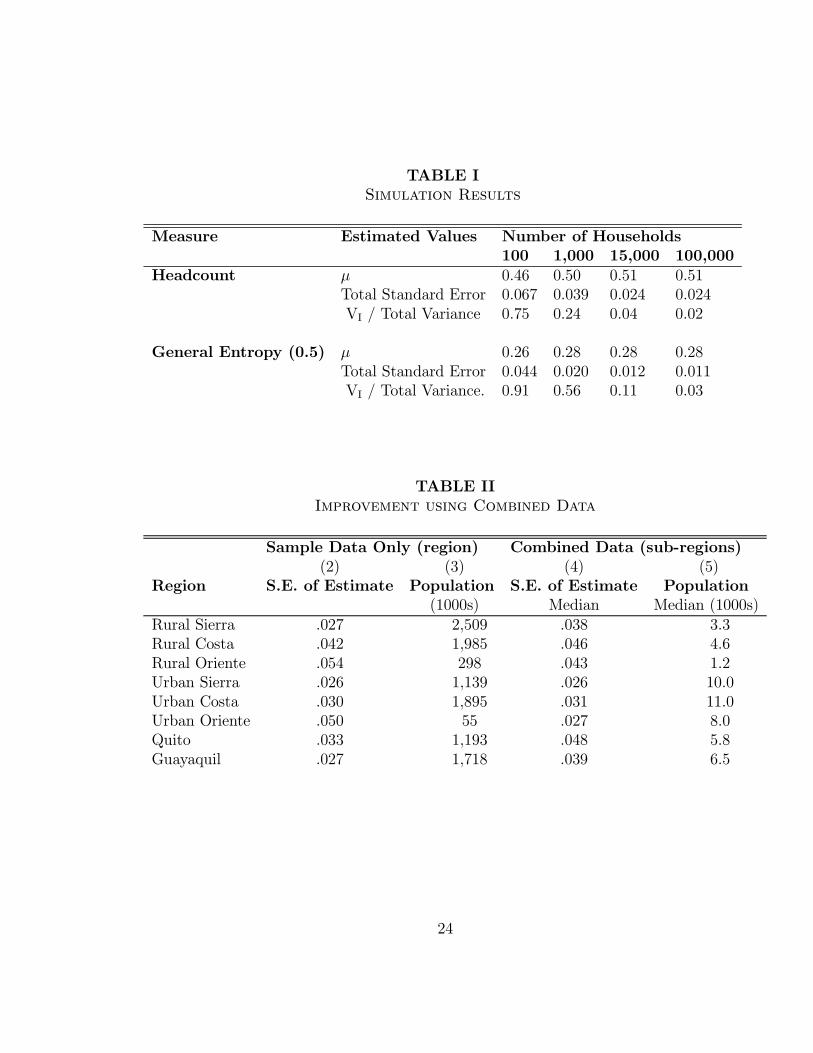
TABLE ISimulation Results
Measure Estimated Values Number of Households100 1,000 15,000 100,000
Headcount ¹ 0.46 0.50 0.51 0.51Total Standard Error 0.067 0.039 0.024 0.024VI = Total Variance 0.75 0.24 0.04 0.02
General Entropy (0.5) ¹ 0.26 0.28 0.28 0.28Total Standard Error 0.044 0.020 0.012 0.011VI = Total Variance. 0.91 0.56 0.11 0.03
TABLE IIImprovement using Combined Data
Sample Data Only (region) Combined Data (sub-regions)(2) (3) (4) (5)
Region S.E. of Estimate Population S.E. of Estimate Population(1000s) Median Median (1000s)
Rural Sierra .027 2,509 .038 3.3Rural Costa .042 1,985 .046 4.6Rural Oriente .054 298 .043 1.2Urban Sierra .026 1,139 .026 10.0Urban Costa .030 1,895 .031 11.0Urban Oriente .050 55 .027 8.0Quito .033 1,193 .048 5.8Guayaquil .027 1,718 .039 6.5
24

TYPESCRIPT SYMBOLS LIST
xh (ex)
£ (multiplication)
¯ (beta)
F (calligraphic ef)
§ (capital sigma)
´ (eta)
" (epsilon)
¾ (sigma)
® (alpha)
³ (zeta)
¹ (mu)R(integral)P(summation)
v (nu)
2 (element of)
1 (in¯nity)
! (arrow right)
25

· (kappa)
± (delta)
5 (nabla)
26
Recommended